Article

Comparing DESIS Hyperspectral and Landsat 10 Simulated Superspectral Data for Crop Type Classification in California’s Central Valley

by
Itiya Aneece
1,*,†,
Prasad S. Thenkabail
1,†,
Pardhasaradhi Teluguntla
2,†,
Adam J. Oliphant
1,†,
Daniel J. Foley
1,† and
Jake Lawton
1,†
1
Western Geographic Science Center, U.S. Geological Survey, 2255 N. Gemini Rd., Flagstaff, AZ 86001, USA
2
Bay Area Environmental Research Institute, Western Geographic Science Center, U.S. Geological Survey, 2255 N. Gemini Rd., Flagstaff, AZ 86001, USA
*
Author to whom correspondence should be addressed.
Current address: U.S. Geological Survey, 2255 N. Gemini Rd., Flagstaff, AZ 86001, USA.
Remote Sens. 2026, 18(14), 2282; https://doi.org/10.3390/rs18142282
Submission received: 20 April 2026 / Revised: 25 June 2026 / Accepted: 26 June 2026 / Published: 8 July 2026

Highlights

What are the main findings?
  • The 14 DESIS hyperspectral narrowbands (10 nm) aligned with the Landsat 10 (formerly Landsat Next) spectral dataset produced similar accuracy results to the full 60-band DESIS hyperspectral dataset for classifying crop types. These 14 DESIS narrowbands resulted in higher accuracy than the 14 simulated Landsat 10 superspectral broadbands.
  • When using DESIS narrowbands, Support Vector Machine (SVM) resulted in higher accuracy than Random Forest (RF).
What are the implications of the main findings?
  • A carefully selected set of 14 DESIS hyperspectral narrowbands (10 nm) can achieve classification accuracy comparable to those obtained using all 60 DESIS narrowbands across the 400–1000 nm range. These 14 strategically positioned narrowbands classified crop types with higher classification accuracy than the corresponding 14 Landsat 10 superspectral broadbands within the same spectral range.
  • This study underscores the importance of multi-temporal imagery across the full crop-growing season for achieving more detailed and accurate crop type classifications. Such temporal coverage is more feasible with the planned Landsat 10 routine acquisition of broadband imagery than with task-based hyperspectral collections.

Abstract

To advance crop type mapping in support of global food and water security, this study compared three spectral configurations: (A) the full 60-band DLR Earth Sensing Imaging Spectrometer (DESIS) hyperspectral narrowband (HNB) dataset, (B) a 14-band subset of DESIS-derived HNBs aligned with the planned Landsat 10 (formerly Landsat Next) spectral configuration (400–1000 nm), and (C) DESIS-based simulations of Landsat 10 superspectral broadbands. The analysis was conducted in California’s Central Valley, hereafter referred to as “the Central Valley”, during the peak growing month of August. DESIS imagery from August 2021, 2022, and 2023 was used sequentially for model development, testing, and independent validation. Over these three years, DESIS provided extensive hyperspectral coverage of much of the 4 million hectares in the Central Valley’s. Analyses were performed on Google Earth Engine using two pixel-based supervised classifiers, Random Forest (RF) and Support Vector Machine (SVM), to differentiate three major crop classes: row crops, grapes and tree crops, and winter wheat/fallow/other. The highest overall accuracy (86%) was achieved using SVM in combination with either the full DESIS hyperspectral dataset or the 14 DESIS narrowbands corresponding to Landsat 10. This finding aligns with earlier studies showing a small number of strategically positioned narrowbands can be optimal for crop type classification. Use of the narrowband datasets resulted in substantially higher accuracy (overall accuracy of 86%) compared to the simulated Landsat 10 broadbands (overall accuracy of 75%), supporting previous studies highlighting the utility of narrowbands. Despite the high accuracy using August imagery, the study indicates more granular crop type classification will require multi-temporal observations spanning the full phenological cycle (June–October), especially for a large number of crop classes. Acquiring task-based hyperspectral imagery over such large areas throughout the growing season remains operationally challenging. In contrast, Landsat 10 superspectral imagery could provide routine coverage across seasons and years that is practical and scalable for future large area crop type mapping and agricultural monitoring.

1. Introduction

1.1. Importance of Agricultural Studies

Food and water security issues are being exacerbated by population growth and by changes in temperature, precipitation, and global dietary preferences [1,2,3,4,5,6]. The current global population of over 8.2 billion continues to rise, with approximately 8.2% (673 million people) experiencing hunger [7,8]. Meeting increasing food demands may require a 25–70% increase in production by 2050 [6], making the mapping and monitoring of agriculture and associated water use imperative [9,10], especially in irrigated lands, which provide 40% of food while comprising only 20% of agricultural land [6]. Monitoring crop locations, health, and resource use can facilitate estimates of food and water availability and support farmer decision-making around resource allocation such as water, helping to maximize yields while promoting sustainable agricultural practices [11,12,13]. Traditional ground surveys are labor-intensive, expensive, and sometimes not feasible [12]. In contrast, remote sensing provides a non-destructive, repeatable, and cost-effective way to monitor large areas rapidly enough to inform decision-making [3,12,13,14,15]. Numerous remote sensing platforms have been used for agricultural studies [16].

1.2. Multispectral Remote Sensing of Agriculture

Studies using multispectral broadband sensors such as Landsat, Sentinel, and Planet Labs Public Benefit Corporation (PBC) Doves and SuperDoves have evolved extensively over the past five decades, reflecting advances in sensor technology, spatial/spectral resolution, revisit frequency, and analytical methods (e.g., big data analytics, artificial intelligence, and cloud computing) [17,18,19,20,21,22,23]. Landsat sensors specifically have been used for numerous cropland mapping efforts regionally, nationally, and globally since the launch of Landsat 1 in 1972 [24,25,26,27,28]. Eight successive Landsat missions with improvements in design, preprocessing, and analysis-ready data products have provided continuity of high-quality consistent data [27]. These data facilitate large-scale crop monitoring, land cover mapping, environmental change detection, disaster planning and management, and resource management [27,29,30].

1.3. Hyperspectral Remote Sensing in Agriculture

Hyperspectral approaches further facilitate crop type mapping by collecting data in hundreds of narrow and contiguous spectral bands [31]. The spectral profiles are sensitive to subtle differences in chemical composition and structural characteristics, allowing more precise estimation of plant biophysical and biochemical characteristics [32,33]. Hyperspectral remote sensing has been used to study many aspects of agriculture, such as the detection of stress due to pests, disease, and water/nutrient limitations; assessment of crop quality; estimation of crop biomass/yield; and classification of crop types [1,11,12,31,32,33,34,35,36,37,38].
Further facilitating agricultural studies, several hyperspectral sensors have recently been launched. This includes government-led sensors such as the Italian Space Agency’s Precursore IperSpettrale della Missione Applicativa (PRISMA) [39,40,41,42,43,44,45]; the German Aerospace Center DLR (Deutschen Zentrums für Luft- und Raumfahrt) Earth Sensing Imaging Spectrometer (DESIS) [46,47,48,49,50] and Environmental Mapping and Analysis Program (EnMAP) [11,51,52]; and NASA’s Plankton, Aerosol, Cloud, Ocean, Ecosystem (PACE) [53,54,55] and Earth Surface Mineral Dust Source Investigation (EMIT) [56,57,58]. Commercial sensors such as Planet Lab’s Tanager [59,60] and Pixxel’s Firefly constellation [61,62] are also increasing hyperspectral data availability. There are also several upcoming sensors, such as NASA’s EAGLE sensors based on the Surface Biology and Geology (SBG) mission [63] and the planned Pixxel Honeybee constellation [61,62].
PRISMA data have been used to detect non-photosynthetic vegetation by emphasizing cellulose and lignin absorption features and calculating band depth [43]. PRISMA imagery has also been integrated with PROSAIL-PRO simulations to develop regression models for estimating several crop traits: leaf chlorophyll/nitrogen/water content, leaf area index, and canopy chlorophyll/nitrogen/water content [45]. DESIS data have been applied to differentiate mono-cropping and inter-cropping in maize fields using random forest [48,49]. Farmonov et al. [50] combined DESIS and lidar data for crop classification using convolutional neural networks. Hyperion and EnMAP data have supported the mapping of mine waste surfaces with the material identification and characterization algorithm (MICA) [52]. Pixxel hyperspectral data have been used to map mangroves [61].
However, preprocessing and analyzing hyperspectral data present many challenges. These include the need for atmospheric correction of some datasets, georeferencing, mitigating the Hughes phenomenon, increased computation time and resources, and the use of advanced machine learning algorithms [1]. The Hughes phenomenon, or the curse of high data dimensionality, describes the need for more samples in order to maintain statistical viability as the number of variables increases [64]. Collecting large numbers of samples can be cost-prohibitive and may be physically, logistically, and/or politically challenging; thus, reducing the number of variables without removing information can help to mitigate this issue. Data redundancy from using too many variables can also decrease classification accuracy, making careful variable selection crucial for hyperspectral data analysis [33]. The number of variables can be reduced through feature engineering using dimensionality reduction techniques such as Principal Component Analysis (PCA), factor analysis, non-negative matrix decomposition, linear discriminant analysis, and minimum noise fraction transformation [1,32,49]. Another method is feature selection, which identifies the most informative bands that are optimal for a given application [1,33,48].

1.4. Superspectral Remote Sensing

Superspectral data such as proposed for the Landsat 10 (formerly Landsat Next) mission [27,63,65,66,67,68] may provide benefits while reducing many of the challenges of hyperspectral data. Landsat 10 will continue the Landsat legacy, with a planned launch in 2031 [63]. The mission will likely greatly increase temporal, spatial, and spectral resolutions compared to previous missions [27,63,67]. Its design will include 26 bands, with most visible; near-infrared and shortwave infrared bands will have a spatial resolution of 10–20 m, while the thermal infrared bands will have a spatial resolution of 60 m [27,63]. Simulated Landsat 10 data have already been successfully used to map minerals [63] as well as to monitor soybean water use and estimate yield [67]. Such pre-launch evaluations are essential because users need to understand expected sensor performance before a mission becomes operational, especially in application areas such as agriculture where planning and continuity are critical. This is particularly important for the superspectral Landsat 10 mission, which is designed with more and narrower bands in the visible to near-infrared region than many existing broadband sensors, fundamentally changing the spectral information content of each band. Evaluation of these characteristics can help to quantitatively assess the practical utility of the planned Landsat 10 superspectral bands for agricultural classification, which will become increasingly relevant as Landsat 10 approaches launch. Simulating Landsat 10 bands using DESIS bands, which are narrower than most spaceborne hyperspectral narrowbands, allows for a clearer understanding of the spectral information captured by the superspectral bands.

1.5. Knowledge Gaps

As remote sensing capabilities continue to advance with hyperspectral and upcoming superspectral missions, they open new opportunities for large-scale agricultural monitoring. Several large-scale crop type mapping efforts are underway [5,11,16,69,70,71,72,73,74,75,76,77,78,79,80,81,82,83,84,85,86,87,88,89,90]. However, there is currently no high-resolution (30 m) publicly available global crop type product because such a product is difficult to create [90]. Developing such a high-resolution product will require leveraging new remote sensing datasets such as hyperspectral and upcoming superspectral imagery as well as implementing advanced methods and techniques on cloud platforms to analyze large volumes of data. It will also require large amounts of high-quality annotated training data for model development [1,5,12,33,91]. These annotated samples are especially important for agricultural studies, where crop signatures vary widely across environmental conditions, management regimes, and seasons [1,33]. Several national spectral libraries are in development to help capture this variability [36,92,93,94,95]. A comprehensive global spectral library of agricultural crops in various growth stages, growing conditions, agroecological zones, and management regimes would support global classification efforts [36] and inform issues around global food and water security. This research contributes to a broader global initiative, the Global Hyperspectral Imaging Spectral-library of Agricultural crops (GHISA) [96,97,98], while focusing on California’s Central Valley, hereafter referred to as “the Central Valley”.

1.6. Overarching Goal and Objectives

Our overarching goal is to assess the ability of superspectral Landsat 10 data (simulated from DESIS hyperspectral data) compared with DESIS data in order to classify three irrigated agricultural crop classes (Row Crops; Grapes + Tree Crops; Winter Wheat + Fallow + Other) across the Central Valley. For this, we had the following specific objectives:
  • Build spectral libraries of three crop classes throughout the Central Valley using (a) all DESIS hyperspectral narrowbands (HNBs), (b) 14 DESIS HNBs corresponding with Landsat 10 bands, and (c) DESIS-derived Landsat 10 simulated superspectral bands.
  • Use spectral libraries to build training, testing, and validation datasets for machine learning models.
  • Compare classification performance across the DESIS and Landsat 10 datasets.
  • Compare classification accuracy across two pixel-based machine learning algorithms (SVM and RF).

2. Materials and Methods

2.1. Study Area

California is one of the largest agricultural states in the United States, with high water demands for its extensive irrigated agricultural areas [71,99]. The most prevalent crops grown in California by acreage are almonds, grapes, alfalfa, corn, pistachios, walnuts, citrus, rice, winter wheat, tomatoes, and cotton [71]. In 2022, those acreage percentages were 16.3% for almonds, 7.9% for grapes, 6.1% for alfalfa, 5.7% for corn, 5.7% for pistachios, 4.6% for walnuts, 3.2% for citrus, 2.7% for rice, 2.5% for wheat, 2.4% for tomatoes, and 1.4% for cotton [71]. Approximately 80% of California’s water use is for agriculture [74], which is primarily located in the Central Valley, a large flat basin that dominates the state’s interior. The Central Valley comprises 75% of California’s irrigated land and produces over 50% of U.S.-grown fruits, nuts, and vegetables [71]. It also produces 99% of U.S.-grown almonds, pistachios, and grapes. The already-high water demand for agriculture in the Central Valley is rapidly increasing while water sources decline [74]. Droughts during 2012–2016 and 2020–2022 have led to drying of wells, while over-use of water from aquifers is also stressing the water supply [74]. In addition, perennial crops such as nut and fruit trees are prevalent in the Central Valley. These crops have high water demand and cannot be let fallow in drought years [74]. The impacts of droughts are exacerbated in California by increasing temperatures. Higher temperatures increase evaporation, which depletes water reservoirs in snowpack, soil, and surface water bodies [74]. Higher temperatures also increase evapotranspiration and thereby agricultural water demands [74]. Due to DESIS image availability, this study focused on the San Joaquin Valley within the Central Valley.

2.2. Remote Sensing Data

2.2.1. DESIS

The DLR (German Aerospace Center) Earth Sensing Imaging Spectrometer (DESIS) sensor is onboard the Multi-User System for Earth Sensing (MUSES) platform of the International Space Station (ISS) [100]. DESIS collects data at 30 m spatial resolution in the visible to near-infrared region (400 to 1000 nm) in 235 narrow spectral bands with 2.55 nm bandwidth [100]. DESIS products are available orthorectified and in surface reflectance [100]. The DESIS 4-bin product consists of 60 bands with 10 nm bandwidths [101]. DESIS data are often used for agricultural research [49,50,102,103].
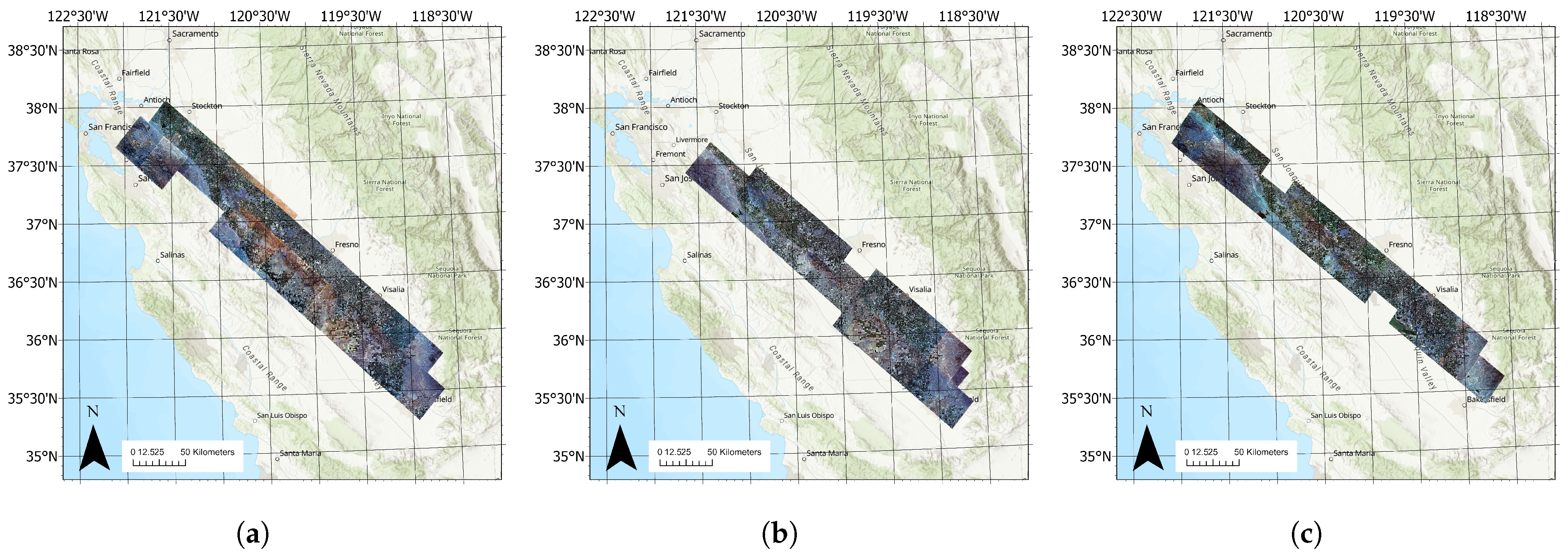
DESIS image acquisition is task-based, as opposed to continuous data collection for multispectral sensors. The authors requested and acquired DESIS data over much of the Central Valley, encompassing nearly 4 million hectares, for the months of August for three years (2021–2023). August is an ideal period for differentiating crops because cotton plants are still flowering, tomatoes and grapes are fruiting, and almonds and pistachios are in nut formation. A total of 75 images from August 2021, 2022, and 2023 in the Central Valley were used to generate mosaics for those years (Figure 1 and Table 1). Twenty-eight images from 2021 (five from 16 August, one from 20 August, eleven from 24 August, and eleven from 28 August) were used to generate the 2021 mosaic. Twenty-four images from 2022 (eleven from 20 August, five from 24 August, and eight from 28 August) were used to generate the 2022 mosaic. Twenty-three images (eleven from 14 August and twelve from 18 August) were used to generate the 2023 mosaic. These images were georeferenced and mosaicked in ArcGIS Pro [104] before ingesting them as assets into Google Earth Engine (GEE) [105].

2.2.2. Landsat 10

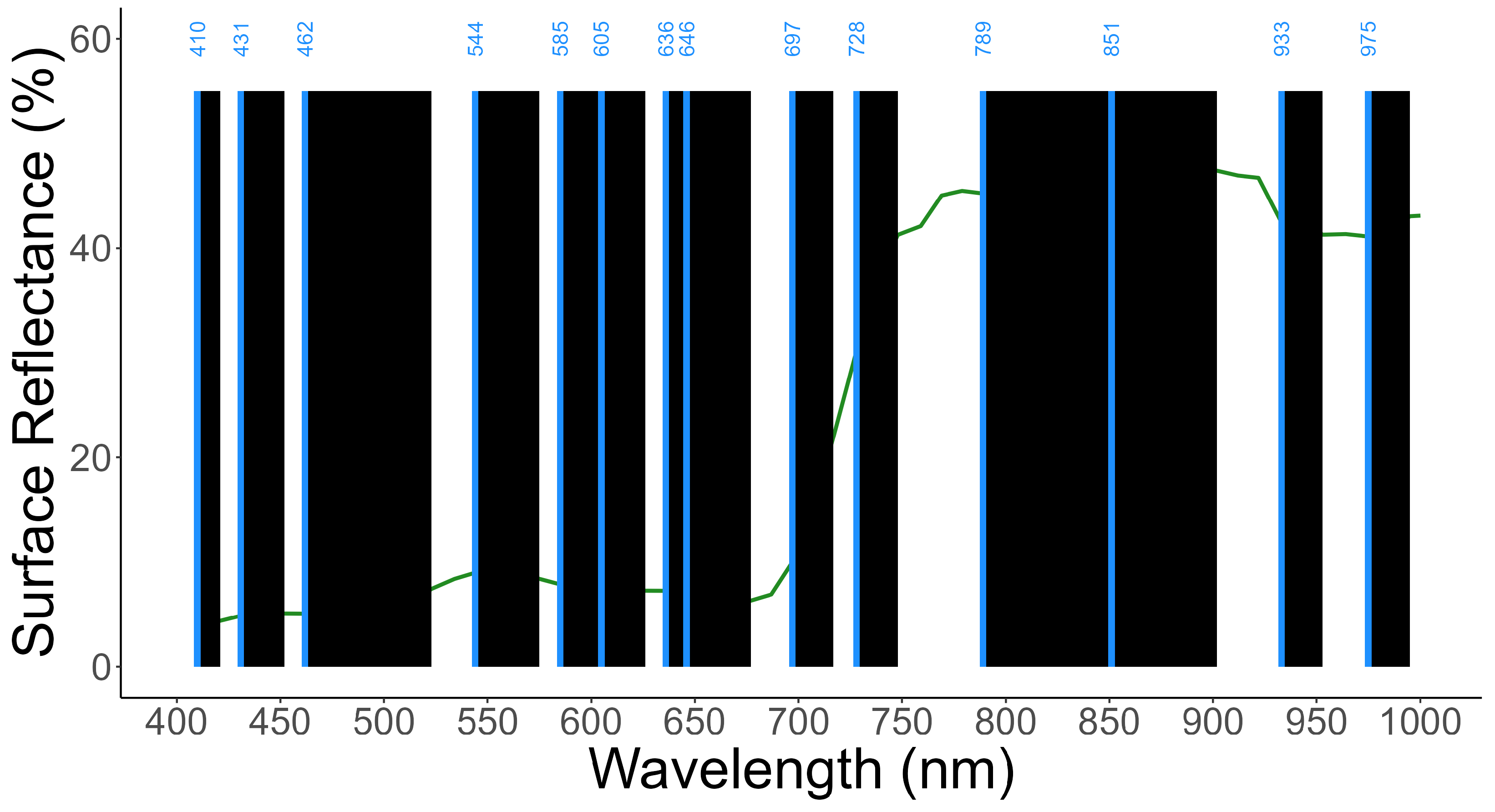
Previous studies have simulated Landsat 10 bands to assess the potential use of these data for various applications [63,68]. In this research, we used the bands for the proposed Landsat 10 mission to assess how these bands would perform for agricultural applications. The DESIS 4-bin image mosaics were used to simulate Landsat 10 data in two ways. In the first method, the Landsat 10 bands (Table 2 and Figure 2) were used to select 14 corresponding DESIS narrowbands (referred to here as Landsat 10 narrowbands). In the second method, DESIS narrowbands within the Landsat 10 band ranges were averaged to simulate the Landsat 10 broadbands (referred to here as Landsat 10 broadbands). A boxcar simulation method was used because Landsat 10 has not yet been launched and we do not yet have information on signal-to-noise ratios, band-center misalignment, or spectral response functions that would enable more nuanced simulation.

2.3. Reference Data

Crop type reference data were acquired from the United States Department of Agriculture (USDA) National Agricultural Statistics Service (NASS) Cropland Data Layer (CDL) [84]. The CDL provides 30 m land cover data for the conterminous U.S. (CONUS) from 1997 to 2023, including over 100 land cover types, with a focus on crop types [16,91]; 10 m data have been made available for 2024 to present. The annual product is generated using multiple data sources, including sensors like Landsat 8/9 and Sentinel 2A/2B, ground reference USDA Farm Service Agency (FSA) Common Land Unit (CLU) data, and the U.S. Geological Survey (USGS) National Land Cover Database (NLCD) [16]. Before 2007, the CDL was produced using a maximum likelihood classifier; afterward, NASS transitioned to a decision tree approach [106]. Because this operationally validated dataset incorporates FSA ground survey records, it is widely considered the most authoritative and spatially explicit crop type dataset available for the United States. Its long-term consistency, national coverage, and annual validation make it the de facto standard for agricultural remote sensing research, as demonstrated by its extensive use in hundreds of peer-reviewed studies [16,91,107,108,109,110,111]. The use of USDA Cropland Data Layer (CDL) as reference data for training, testing, and validating crop type classification models is critically important, yet it must be recognized that CDL itself contains inherent uncertainties that propagate into any models derived from it. For California, the CDL reported overall classification accuracy of 78.4%, 81.4%, and 80.7% for 2021, 2022, and 2023, respectively (Table 3). Certain classes, particularly winter wheat and other non-alfalfa hay, exhibited lower producer’s and user’s accuracy, ranging from 62.1% to 76.4% across years. For the remaining study crops, producer’s accuracy ranged from 68.4% to 92% and user’s accuracy from 74.2% to 90.9%, indicating stronger but still imperfect performance. These uncertainties underscore the need for high-quality and field-collected reference data capable of reducing classification noise and improving the reliability of spectro-biophysical models. While CDL remains the gold standard for national-scale crop type mapping, largely because collecting consistent country-wide reference data is logistically complex and resource-intensive, its limitations become more pronounced when developing fine-scale or high-accuracy models. The most effective pathway toward generating high-fidelity reference datasets is through systematic field campaigns conducted throughout the growing season. Such campaigns enable precise crop identification, capture phenological variability, and provide robust validation datasets. Although these efforts require substantial investment in terms of time, personnel, and resources, they are justified when the goal is to develop high-accuracy transferable models. Importantly, field-validated models built across representative years, including normal, drought, and wet conditions, can subsequently be used to automate crop type mapping for independent years with far greater confidence.
Alongside the CDL, we also used the California Department of Water Resources (CADWR) Statewide Crop Mapping Dataset’s field boundaries [71,114] to obtain field centroids and avoid boundary effects in sample selection. These field boundaries are derived using the USDA National Agriculture Imagery Program (NAIP) dataset for field boundary delineation and Landsat images and field data for crop classification and water use estimation [16,71]. By using CADWR boundaries to extract field centroids and CDL labels to assign crop types, we effectively combine two independent high-quality datasets, thereby reducing reliance on any single source and mitigating any concern about using CDL alone. This dataset has also been used extensively in agricultural research [16,115].
The DESIS imagery used in this study covers a very large portion of the Central Valley, and acquiring ground survey data at this scale would be prohibitively expensive and logistically infeasible. Using existing products such as CDL and CADWR is a cost-effective way to obtain numerous high-quality samples across a large spatial extent [91]. Therefore, these datasets provide a scientifically defensible and operationally practical alternative for large area validation. Finally, the consolidation of crop types into three broader classes further reduces the likelihood of CDL misclassifications affecting our results. CDL accuracy is highest for major crop groups, and grouping similar crops (e.g., grapes + tree crops; winter wheat + fallow) aligns with known CDL strengths and minimizes the impact of class level confusion. Together, the use of CDL, CADWR field boundaries, centroid-based sampling, and class consolidation provides a robust, multisource, and scientifically defensible validation framework appropriate for large-scale hyperspectral classification studies.

2.4. Image Processing

DESIS 4-bin surface reflectance images for August 2021–2023 were downloaded from the Teledyne Brown data portal [101] and were georeferenced and mosaicked in ArcGIS Pro [104]. The mosaics were then ingested into GEE as assets for analysis and masked using the Global Food Security-Support Analysis Data (GFSAD) Landsat-Derived Global Rainfed and Irrigated-Cropland Product 30 m (LGRIP30) [116] to remove most non-cropland pixels, although some remained unmasked. DESIS Band 1 was removed due to noise. The mosaics were then rescaled to 90 m to account for information from neighboring pixels and reduce computational loads. Preliminary analyses on subsets of the data showed that rescaling DESIS imagery from 30 m to 90 m slightly increased classification accuracy. This improvement is consistent with hyperspectral classification theory: aggregating to 90 m reduces pixel level noise, minimizes mixed-pixel effects at field boundaries, and produces more stable spectral signatures that better represent the dominant crop type within each field. Because our study focuses on three broad crop classes, the smoother and more homogeneous spectra at 90 m increased class separability and reduced intra-class variance, leading to more robust performance of RF and SVM classifiers. Additionally, the computational efficiency gained from using 90 m hyperspectral data over a large area enabled more extensive experimentation and parameter tuning. Together, these theoretical considerations and empirical tests justify the use of 90 m resampled data in this study. Landsat 10 bands were then simulated using the DESIS mosaics. Lastly, in the resulting 2023 classification maps, the mode classification for each field (based on CADWR field boundaries) was used to classify the entire field.

2.5. Sample Generation

The field boundaries were used to select field centroids to avoid field boundary effects in samples. Data from the DESIS mosaics were extracted from a random subset of centroids and visually filtered for outliers. The selected sample locations were then used in the models. The 2021, 2022, and 2023 data were used for training, testing, and validating the classification models, respectively. An initial classification was done by crop type; however, classification results showed low accuracy, with high levels of confusion among certain crop types (shown in Section 3 below). Upon inspection of the spectra across classes and errors of omission and commission from the initial classification, crop types were consolidated into three crop classes: (1) Row Crops (e.g., cotton, hay, tomatoes, and other crops); (2) Grapes + Tree Crops (e.g., grapes, almonds, pistachios, and other tree crops),; and (3) Winter Wheat + Fallow + Other (e.g., winter wheat, fallow/idle fields, and other cover classes such as developed areas and wetlands). Winter wheat was combined with fallow because it has already been harvested by August, so fields often resemble fallow fields spectrally. Grapes and tree crops also often have similar spectral signatures.
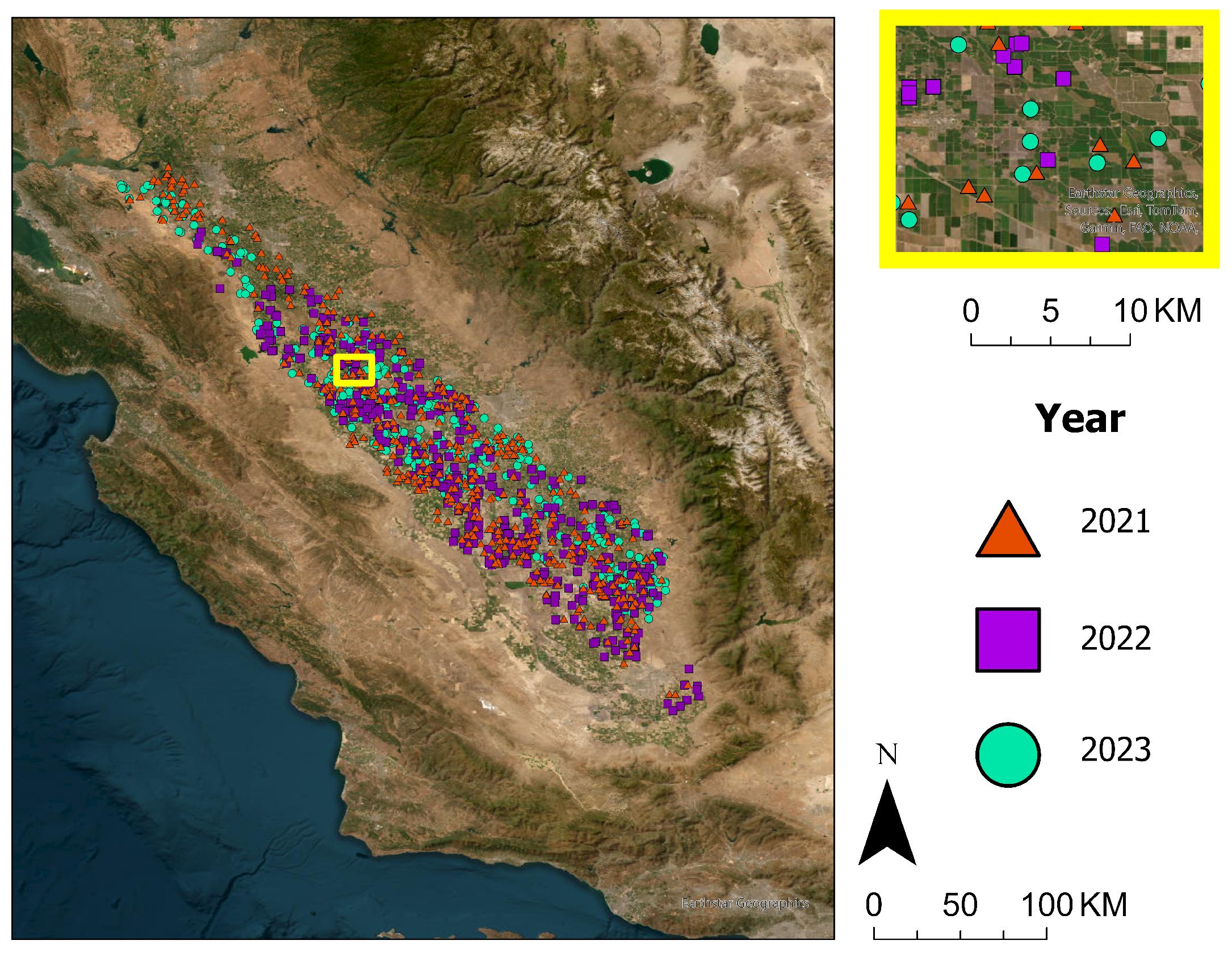
Out of the field centroids, 150 samples for each crop class and year were selected for classification in order to avoid complications from sample imbalance [1,11], for a total of 450 samples for each year and an overall total of 1350 samples (Figure 3). The decision to use 150 samples per class per year was driven by the need to maintain balanced class representation, which is essential for avoiding bias in supervised classification and accuracy assessment. Because the three crop classes differ substantially in their spatial prevalence, the least-abundant class constrained the maximum number of samples that could be drawn uniformly across all classes. Selecting a larger number of samples for the more common classes would have introduced imbalance and inflated accuracy metrics, which is a well-documented issue in remote sensing classification [1,11]. Thus, the final sample size represents the largest balanced subset that could be used without compromising statistical fairness, representing a tradeoff between ensuring statistically meaningful accuracy estimates and maintaining class balance across years and crop categories. Training, testing, and validation samples were spatially distributed across the study area (Figure 3). This spatial dispersion is critical because it ensures that the sample sets capture the full heterogeneity of agricultural landscapes in the Central Valley, including differences in field size, crop management practices, soil conditions, and micro-climatic gradients. Spatially clustered samples can artificially inflate or deflate accuracy metrics; therefore, the demonstrated spatial spread strengthens the robustness of the evaluation. Finally, the use of field centroids rather than arbitrary pixel locations further reduces boundary effects and mixed-pixel contamination, which are common sources of error in agricultural classification. This centroid-based approach ensures that the extracted spectra represent the interior of fields, where crop signatures are most homogeneous and least affected by edge effects. Together, these methodological choices such as the balanced sampling, visual sample quality checks, spatially-distributed samples, and centroid-based extraction provide a scientifically defensible and statistically robust foundation for using 450 samples per year to assess classification performance.

2.6. Machine Learning Algorithms

Machine learning algorithms were run in GEE, which enables large-scale repeatable workflows leveraging Google’s server-side computation resources [117]. GEE has been used extensively in agricultural research [5,6,13,15,80,91,117,118,119,120] and is particularly powerful for geospatial data analyses [117]. The platform provides automatic parallel computing and offers several datasets through its data catalog [15,117]. The platform also includes several easily implementable machine learning algorithms built into the JavaScript Application Programming Interface (API) [15,117], including Random Forest (RF) [2,9,10,14,120,121,122,123] and Support Vector Machine (SVM) [3,4,15,124,125,126,127], which are often used in agricultural research [11,15,16,31,33,91].
RF and SVM were selected for this study because they are well established, transparent, and widely used in sensor comparison studies, allowing us to isolate sensor performance rather than confounding the analysis with complexities of model architecture. While more complex deep learning methods such as neural networks exist, traditional machine learning algorithms have lower computational demands, reduced parameter tuning, shorter run times, and a relatively smaller requirement of reference data [11,31]. Traditional machine learning algorithms are versatile, effective, and widely used in agricultural studies [3]. Their integration into the GEE JavaScript API makes them easy to implement, scale, and share within the research community.
The RF algorithm is an ensemble learning method that constructs a collection of decision trees and classifies samples using a majority vote [37,121]. It is robust to high data dimensionality, large datasets, nonlinear relationships, overfitting, and outliers [10,15,37]. RF has been used successfully in both classification and regression analyses, and is straightforward to implement and interpret [15,120]. In this study, the number of trees was set to 250 for computation efficiency, and out-of-bag fraction was set to 0.5. Other parameters were optimized using grid search, with the minimum leaf population ranging from 5 to 100 and the maximum number of nodes ranging from 5 to 500. For the analysis using all DESIS bands, the number of variables tested ranged from 10 to 55; for the Landsat 10 band analyses, the number ranged from 6 to 14.
SVM projects data in an n-dimensional space and determines a hyperplane that best separates the classes [36,124,125]. This hyperplane is defined by the samples closest to it, referred to as support vectors [15]. Alongside a linear kernel, several other kernels make SVM well suited for handling nonlinear relationships [124,125]. The linear kernel is available in GEE, as are the nonlinear radial basis function (RBF), polynomial, and sigmoid kernels. SVM is frequently used for classification, regression, and outlier detection [3]. In this study, we tested the linear, RBF, and first-degree polynomial kernels (with coefficient = 0) for classification. Cost and gamma parameters were optimized using grid search, with cost values ranging from 1 to 1000 and gamma values ranging from 0.0001 to 0.1.

3. Results

3.1. Spectral Library of Crops

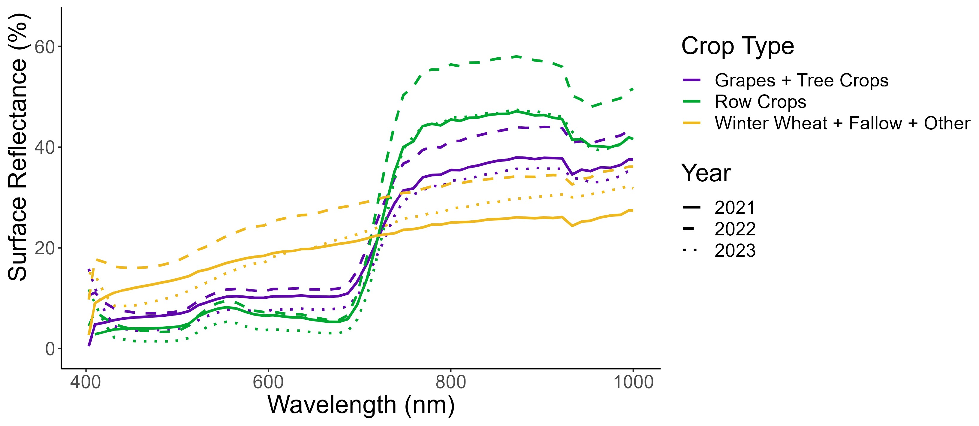
Samples for the three crop classes were used to generate hyperspectral libraries of agricultural crops (Figure 4) for the training year (2021), testing year (2022), and validating year (2023). These libraries make substantial contributions to the global hyperspectral imaging spectral library of agricultural crops (GHISA, [128]) developed by this team. Spectral averages within each year showed that the three classes were spectrally distinguishable from one another. The average spectral profile for Winter Wheat + Fallow + Other largely resembled a soil line, with high reflectance in the visible region and low reflectance in the near-infrared region. Reflectance of row crops in the visible region was often lower than that of the Grapes + Tree Crops class, while the opposite was observed in the near-infrared region. Thus, row crops often exhibited higher “greenness” than grapes and tree crops, most likely due to greater influence from inter-row soil signatures in vineyards and orchards than in row crop fields. The average spectral profiles across years were similar within each class, demonstrating relative inter-annual consistency.

3.2. Machine Learning Classification Using DESIS and Landsat 10 Simulated Data

An initial classification across the nine classes (cotton, fallow, grapes, hay, other crops, tomatoes, tree crops, winter wheat, and other) with all DESIS bands resulted in low accuracy using RF (Table 4) and SVM (Table 5). Using RF resulted in an overall accuracy of 28%, with producer’s and user’s accuracy results of 5–50% and 11–54%, respectively. Using SVM, the overall accuracy was 39%, with producer’s accuracy of 9–68% and user’s accuracy of 25–78%. These low classification accuracy results are most likely due to a lack of temporal images covering multiple dates during the phenological growth stages of the crops. This exploratory analysis provided us with information on the most commonly confused crop types for subsequent analysis. For example, cotton and hay were often confused; this was likely due to high intra-class variability, especially in hay, where cutting cycles differed by field. Fallow samples and winter wheat were often confused because winter wheat had already been harvested, with fields resembling fallow fields. The confusion between fallow and tree crop samples was driven by young pistachio samples, which were filtered out in subsequent analyses. Grapes were often confused with tree crops, perhaps due to similarities in their growth structures and the layouts of vineyards and orchards. Informed by these exploratory analyses, we aggregated crop types into three crop classes for subsequent classification: (1) Row Crops (e.g., cotton, hay, tomatoes, and other crops); (2) Grapes + Tree Crops (e.g., grapes, almonds, pistachios, and other tree crops); and (3) Winter Wheat + Fallow + Other (e.g., winter wheat, fallow/idle fields, and other cover classes such as developed areas and wetlands).
For RF using all DESIS bands, the highest overall classification accuracy for the test dataset was obtained using 15 variables, a minimum leaf population of 5, and a maximum number of nodes of 10. When using DESIS bands at Landsat 10 band locations, the optimal number of variables was 6, with 10 and 25 as the minimum leaf population and the maximum number of nodes, respectively. When using Landsat 10 simulated broadbands, the highest overall classification accuracy was obtained using 6 variables, a minimum leaf population of 5, and a maximum number of nodes of 10. The polynomial kernel resulted in the highest accuracy results for the SVM classifications. When using all DESIS bands, the best test dataset results were obtained using a gamma of 0.001 and cost of 100. When using DESIS bands at Landsat 10 band locations, the best overall classification accuracy in testing was obtained using a gamma of 0.001 and cost of 10. Lastly, when using Landsat 10 simulated broadbands, the best results were obtained using a gamma of 0.1 and cost of 100. These optimal parameters were then used to classify the validation data.
Training, testing, and validation accuracy results are summarized below (Table 6, Table 7, Table 8, Table 9, Table 10 and Table 11). Although the use of Kappa in remote sensing classification has been debated in the recent literature [129,130], we include it here solely to facilitate comparison with earlier land cover and crop mapping studies, many of which report Kappa as part of their accuracy assessments. Here, we rely more on overall, producer’s, and user’s accuracy as well as on visual comparisons. Using RF, overall training accuracy results across the three datasets (all DESIS bands, the 14 DESIS-based narrowbands corresponding with Landsat 10 bands, and the 14 DESIS-derived Landsat 10 simulated broadbands) were 89–90% (Table 6). Producer’s accuracy ranged from 78 to 97%, while user’s accuracy ranged from 85 to 99%. With SVM, overall accuracy results were 74–91% (Table 7), with producer’s accuracy of 59–99% and user’s accuracy of 62–100%.
For the testing year (2022) and RF, we obtained overall classification accuracy results of 78–80%, with producer’s accuracy ranging from 62 to 95% and user’s accuracy from 71 to 93% (Table 8). Using SVM, overall accuracy results were 79–86%, with producer’s accuracy of 63–97% and user’s accuracy of 71–99% (Table 9).
On the validation dataset, using all DESIS bands and RF led to an overall classification accuracy of 80%, with producer’s accuracy of 74–89% and user’s accuracy of 69–97% (Table 10). When using the 14 DESIS bands corresponding to Landsat 10 bands, the resulting overall classification accuracy was 79%, with producer’s accuracy of 74–88% and user’s accuracy of 68–97%. Using the 14 Landsat 10 simulated broadbands led to an overall accuracy of 79%, with producer’s accuracy of 72–89% and user’s accuracy of 69–97%.
Using all DESIS bands and SVM resulted in a validation overall accuracy of 86%, with producer’s accuracy of 81–92% and user’s accuracy of 79–99% (Table 11). For the 14 DESIS bands, overall classification accuracy was 86%, with producer’s accuracy of 79–93% and user’s accuracy of 79–99%. Using Landsat 10 simulated broadbands, the overall accuracy was 75%, with producer’s and user’s accuracy of 53–96% and 62–86%, respectively.
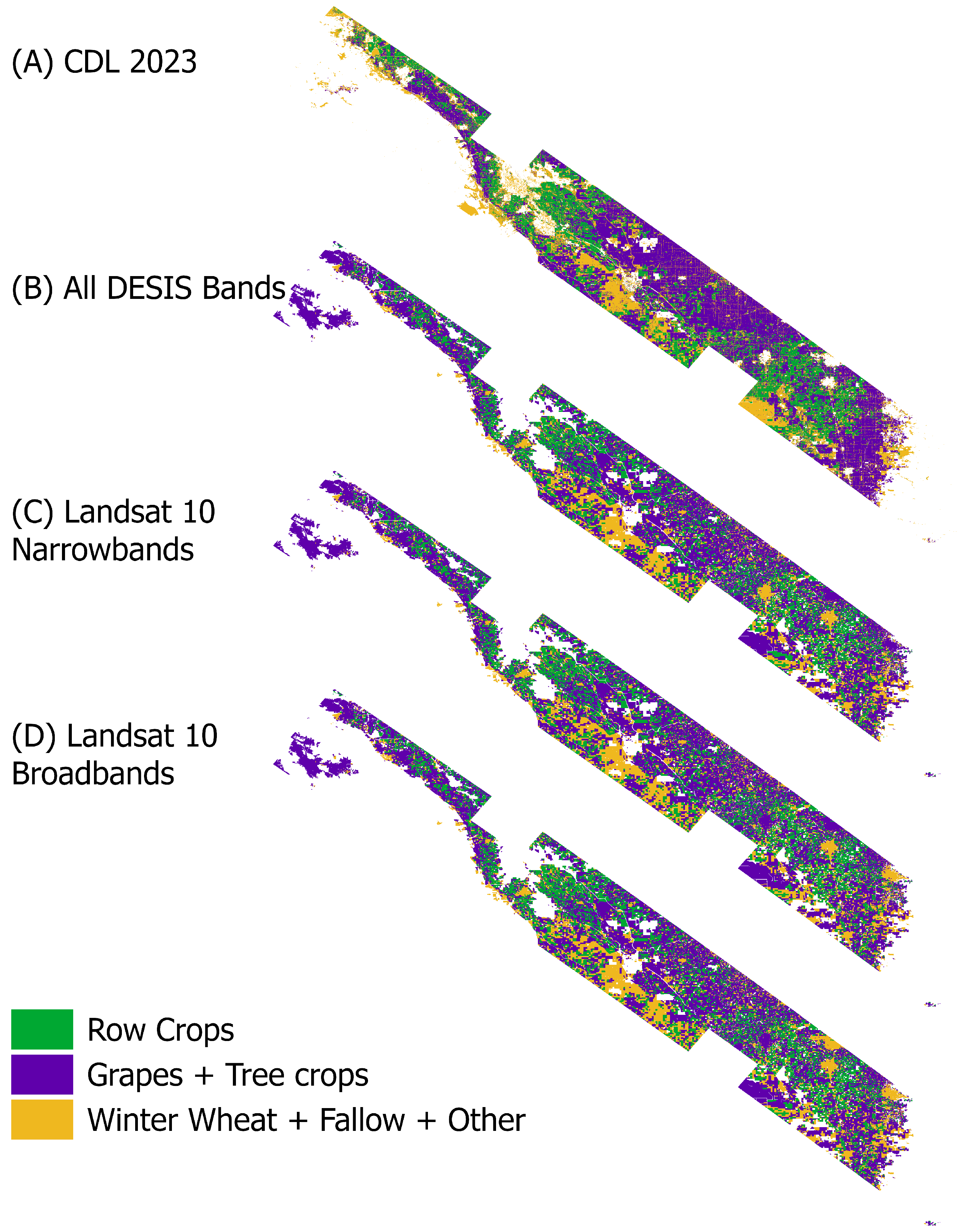
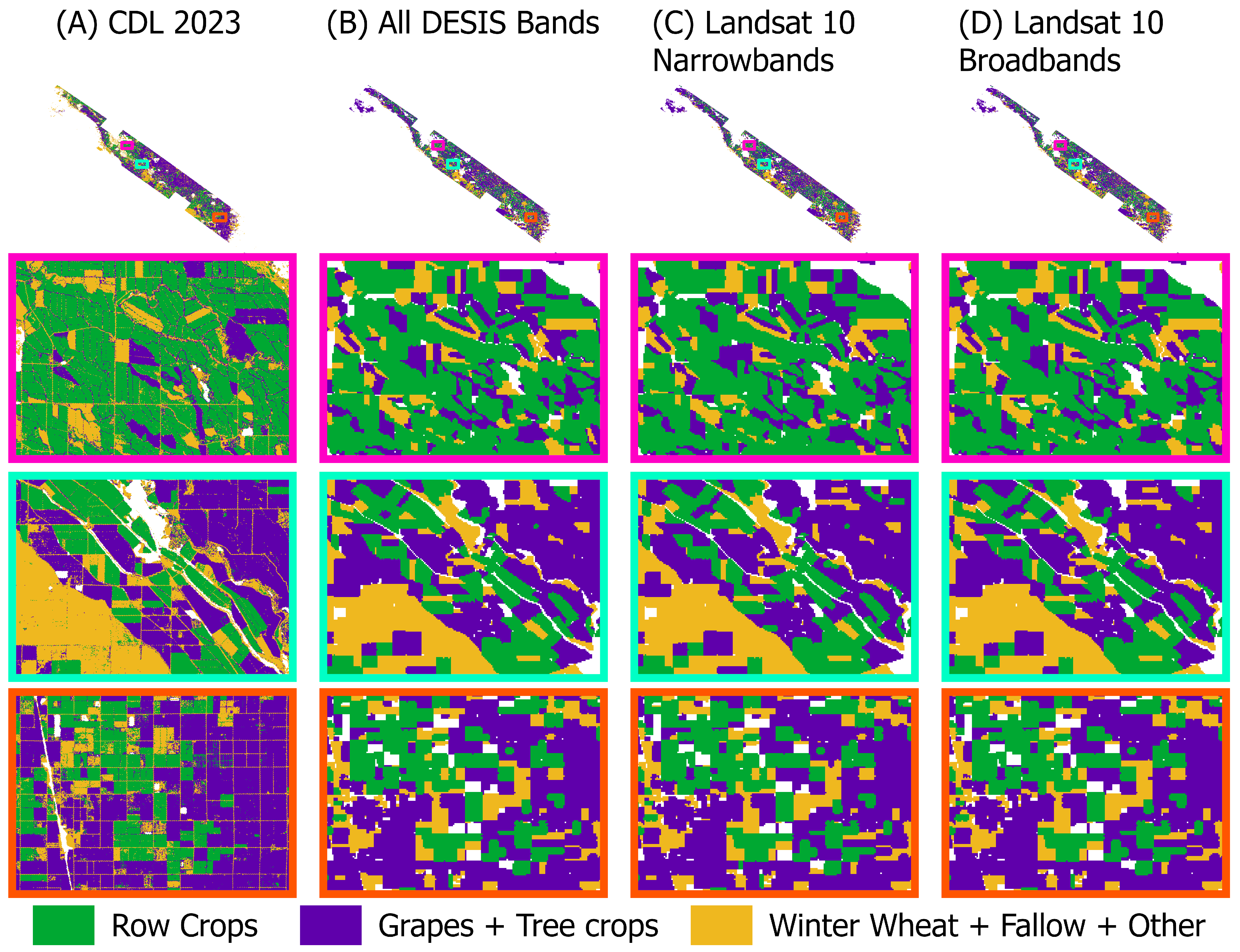
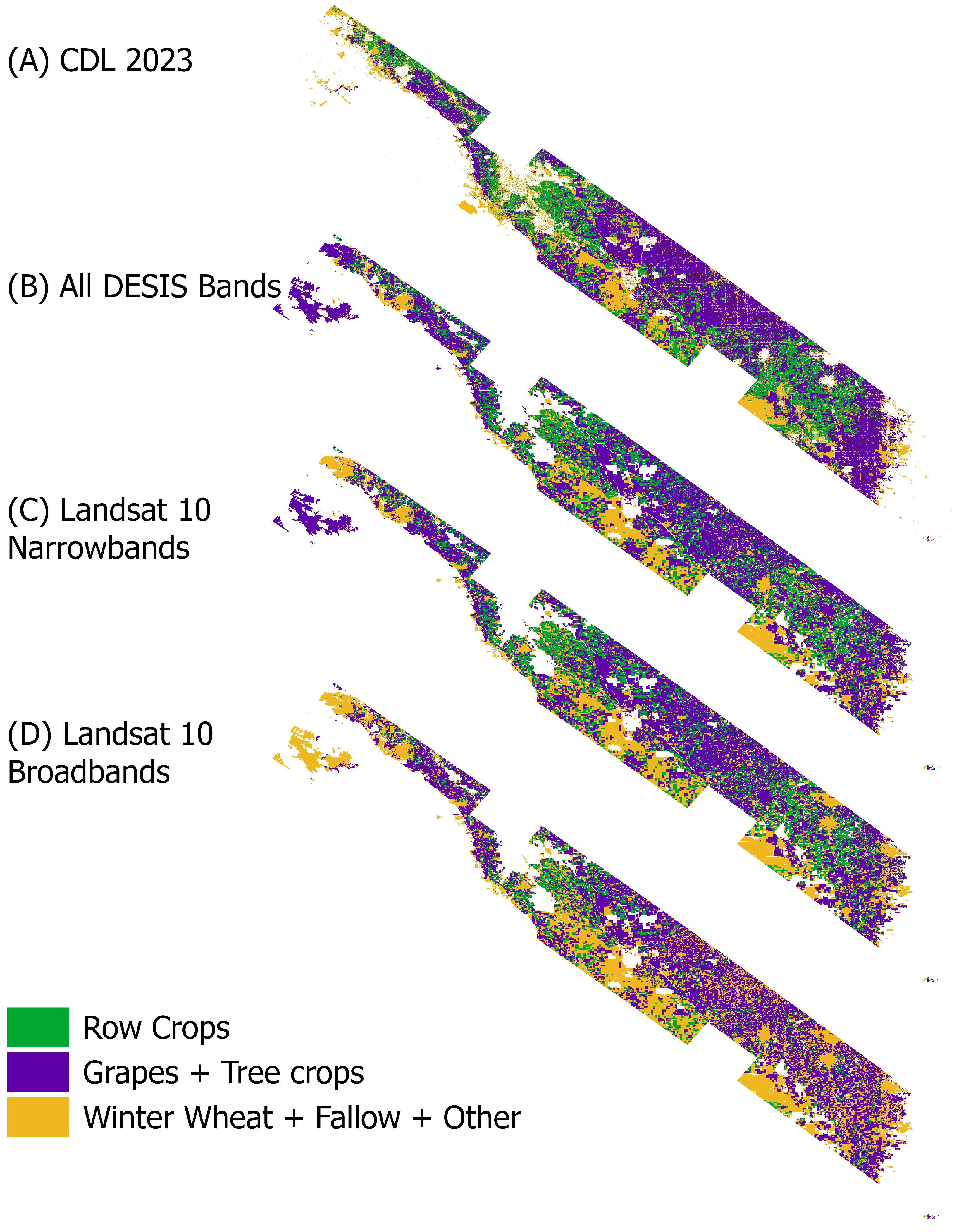
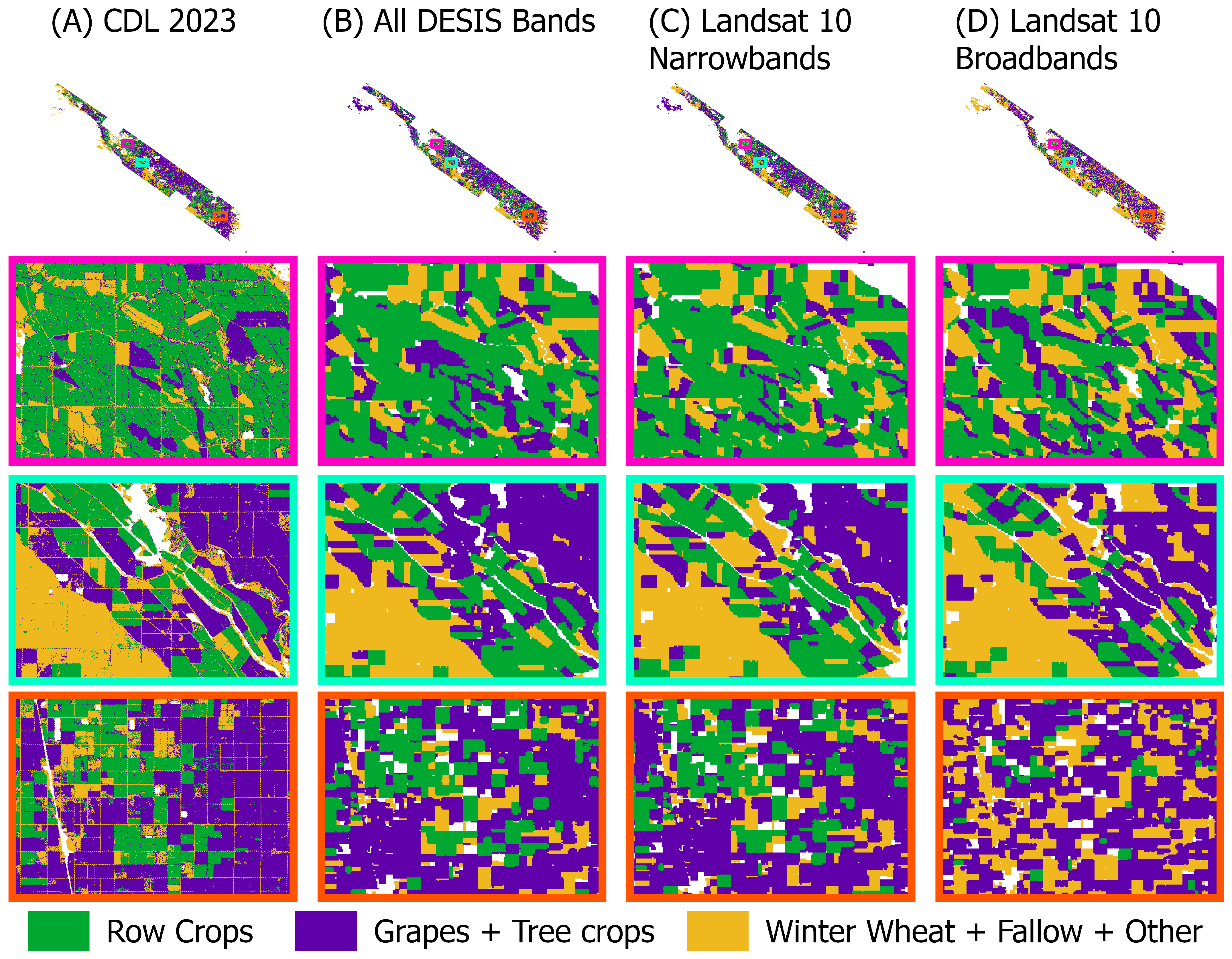
Classification maps for 2023 using RF (Figure 5 and Figure 6) and SVM (Figure 7 and Figure 8) show the comparisons between the results using the three different datasets and classification algorithms. While the overview maps in Figure 5 and Figure 7 may look similar across datasets, subtle differences can be observed in the zoomed-in areas in Figure 6 and Figure 8.
The error matrices for the validation year (2023) are shown below to demonstrate the inter-class confusion (Table 12, Table 13, Table 14, Table 15, Table 16 and Table 17). For example, when using RF, row crops and grapes + tree crops were often confused with each other, perhaps because of similarities in canopy greenness and coverage between the two classes. Some winter wheat + fallow + other samples were often misclassified as tree crops. This is most likely due to some tree and wetland signatures in the other class. This was consistent across datasets when using RF. When using SVM and narrowbands, there was less inter-class confusion and higher overall accuracy; however, when using the simulated Landsat 10 broadbands, many row crops were misclassified as grapes + tree crops.
In summary, SVM resulted in higher accuracy than RF when using narrowbands, with higher consistency in both producer’s and user’s accuracy results across classes. In contrast, when using the DESIS-derived Landsat 10 simulated broadbands, RF was more accurate and consistent than SVM across classes. When comparing datasets, we achieved similar accuracy results across all three when using RF. In contrast, Landsat 10 broadbands provided much lower accuracy when using SVM. For both RF and SVM, the accuracy when using all DESIS bands was similar to when using the 14 narrowbands. In addition, a variable-of-importance analysis of the RF model using all DESIS bands was conducted to determine the most important DESIS narrowbands for classification. The 20 most important bands included those corresponding with 9 out of the 14 simulated Landsat 10 bands, which explains the high classification accuracy results when using only the 14 DESIS narrowbands corresponding with Landsat 10 bands compared to using all DESIS narrowbands (Table 18).

4. Discussion

In this study, we used DESIS hyperspectral images to simulate superspectral Landsat 10 data for classifying three crop classes in the Central Valley (row crops, grapes + tree crops, and winter wheat + fallow + other), for which we built spectral profiles for classification. Spectral averages within each class were similar across years, with observable differences in spectral shapes across the classes. To assess the effect of machine learning algorithm choice on classification accuracy, we compared two pixel-based supervised machine learning algorithms: SVM with different kernels, and RF. We also compared three datasets: using all DESIS bands (except for Band 1), 14 DESIS narrowbands corresponding with Landsat 10 bands, and Landsat 10 simulated broadbands.
The dataset-dependent comparison of RF and SVM from this study contrasts with other studies, in which either RF resulted in higher accuracy than SVM [17,123] or SVM resulted in higher accuracy than RF [124] and where SVM was more consistent in accuracy across classes [124]. When using SVM, we found the polynomial kernel resulted in higher accuracy than the linear and RBF kernels, supporting findings by [3]. In other cases, SVM RBF resulted in higher accuracy than other kernels [127]. Beyond comparing error matrices, visual inspection of classification maps is also important. For example, Traore et al. [15] found that although RF resulted in higher accuracy, SVM had more visually accurate results. In this study, the two performed similarly except when using DESIS-derived Landsat 10 broadbands, in which RF resulted in higher accuracy than SVM. Overall, the optimal algorithm depends on the use case, the number of variables, and complexity of the data.
Classification accuracy when using all DESIS bands was similar to when using 14 narrowbands. This result supports other studies that have also found high overall accuracy with a small number of selected hyperspectral bands, and in some cases even higher accuracy than when using all available bands [33,97]. This might result from the use of all bands introducing noise into the model or leading to overfitting of the training models.
Overall, the highest validation classification accuracy of 86% was obtained using SVM with either all DESIS bands or the 14 narrowbands corresponding to Landsat 10 bands. Nevertheless, misclassifications occurred, especially between row crops and grapes + tree crops. Some winter wheat + fallow + other samples were also misclassified as grapes + tree crops, likely due to tree and wetland samples in the ’other’ category that were not masked out using the LGRIP30 mask [116]. Such misclassifications may result from the challenges inherent in agricultural classification, including inter-class spectral similarities, intra-class spectral variability, and background interference from shadows, crop residues, and soil [31]. Inter-annual differences in environmental conditions and management practices can also affect classification accuracy [31]. Liu et al. [91] similarly found lower accuracy when models were trained on different years than the validation years. All of these challenges were amplified during preliminary analyses aimed at classifying specific crop types. Achieving reliable crop type discrimination will likely require time series hyperspectral or superspectral imagery, more advanced classification algorithms, and/or integration of the additional data sources discussed below. In this study, we identified a subset of crop or vegetation classes that could be automatically and consistently classified across multiple years with the hyperspectral data currently available. As future airborne or spaceborne hyperspectral time series datasets become available, classification can be expanded to include a larger number of classes, ultimately progressing towards robust, scalable, and temporally transferable crop type mapping.
The central objective of this study was to compare DESIS hyperspectral data with simulated Landsat 10 superspectral data using two well established classification algorithms. Although beyond the focus of this study, classification accuracy may be increased in several ways. For example, other algorithms may result in higher inter-annual classification accuracy results. There are various modifications for SVM, including hybridized kernels [125], weighted-tree and ensemble methods [126,127], hyperparameter tuning methods, [125,127], and feature selection methods [3,4]. Advanced deep learning methods may also further increase accuracy [1,17,132]. Commonly used deep learning networks for analyzing hyperspectral data for agricultural applications include Convolutional Neural Network (CNN), Deep Belief Networks (DBN), Autoencoders (AE), Recurrent Neural Networks (RNN), Capsule Networks (CapsNet), Graph Neural Networks (GNN), Morphological Neural Networks (MNN), transformer architectures, and Generative Adversarial Networks (GAN), which can be used for feature extraction, image segmentation, and classification using spatial and spectral information [1,133]. For example, Wu et al. [134] and McCormick et al. [132] used multi-layer perceptrons for crop type mapping. In addition, foundation models made for hyperspectral analysis, such as HyperSIGMA, along with those able to be adapted for hyperspectral analysis such as Prithvi-EO-1.0, may enable more accurate crop type mapping [135]. However, these deep learning and foundation models can be difficult to implement due to requirements around computation, training time, labeled data, energy, and hardware [1]. To ameliorate some of these challenges, transfer learning can also help leverage pretrained models [12,36,91].
Incorporating spatial information through image segmentation for object-based classification [12,13,36] and using field boundaries can also increase accuracy [71]. The CADWR provides field boundaries for California. When expanding this methodology to other states within the US, the USDA NASS and Economic Research Service (ERS) Crop Sequence Boundaries (CSB) dataset can be used, which delineates fields for CONUS using the USDA CDL [71]. Similarly, spectral–spatial CNN–transformer models may increase crop classification accuracy [32,136,137]. Such transformer-based architectures can also be used for self-supervised pretraining of classification models where labeled data are limited [138]; this is particularly the case in agricultural landscapes, where ground truth labels are sparse or expensive to obtain.
Integrating spatiotemporal features (e.g., land cover change, crop rotation, fallowing, and phenological stages) through time series images may also greatly improve crop classification and characterization [11,91,139]. For example, time series data from Sentinel-1 and Sentinel-2 [140,141] and compilations of multispectral images (e.g., PASTIS) [142] have been widely used for crop mapping. Uncrewed Aerial Vehicle (UAV) time series data have also been applied for crop monitoring [143]. These approaches include the use of times series vegetation indices [140,141,143] and structural features [143]. Time series vegetation indices and cultivated area fraction trajectories have also facilitated crop yield estimation [144]. However, spaceborne hyperspectral collections are typically task-based, meaning that acquisitions are limited, irregular, and rarely span an entire growing season. This inherent constraint directly influences the types of analyses feasible with currently available datasets and demonstrates the utility of evaluating sensors such as the superspectral Landsat 10, which will provide consistent and repeated observations with strategically placed narrower bands designed for agricultural applications. By comparing an August DESIS snapshot with simulated Landsat 10 data, this study offers insight into how the upcoming mission may help fill the temporal gaps that spaceborne hyperspectral data currently cannot address. Multi-year training strategies and domain adaptation approaches possible with Landsat 10’s long-term high-frequency data could further enhance the temporal robustness of classification models. In addition, combining single-date hyperspectral data with time series multispectral observations may enhance crop type classification studies [145]. Time series multispectral images may also be used to reconstruct hyperspectral data [146].
Combining optical hyperspectral data with other datasets such as Light Detection and Ranging (lidar), Synthetic Aperture Radar (SAR), multispectral time series, or ancillary data such as meteorological data could increase classification accuracy by leveraging complementary information sources to overcome limitations of single-sensor approaches [11,13,80,91,100]. In this study, we have used DESIS data to simulate Landsat 10 data; however, DESIS data do not include Short-Wave Infra-Red (SWIR) or thermal information, which would be available with Landsat 10. These additional bands, especially SWIR bands, may also increase classification accuracy [147,148,149]. The phenological data in Google DeepMind’s AlphaEarth Foundations embedding product may also increase classification accuracy [150]. Finally, integration of physics-based neural networks that incorporate radiative transfer constraints or vegetation biophysical priors may increase generalization in terms of accuracy across years, sensors, and agro-ecological zones by grounding learned representations in physically meaningful relationships [151].
Object-based approaches and deep learning models play an important and growing role in image classification research; however, we selected traditional machine learning classifiers in this study because they offer a practical balance of accuracy, computational efficiency, and interpretability for our main objective of comparing DESIS with simulated Landsat 10 data. Object-based approaches rely heavily on spatial segmentation and texture, which are less relevant for our centroid-based sampling strategy and spectral comparison focus. Deep learning models are powerful, but require large labeled datasets and extensive computational resources and can introduce black-box behavior that complicates sensor-level comparisons. In contrast, SVM and RF provide high classification accuracy with limited training data and interpretable results that allow us to isolate the effects of spectral information content. Alternative approaches such as object-based methods or deep learning could certainly be explored in future work, particularly as larger labeled datasets and hyperspectral foundation models become available, but the machine learning techniques used here were selected to achieve the specific goals of this analysis.
Wavelength bandwidth, Spectral Response Functions (SRF), and image noise are important factors that can influence the robustness of the classification accuracy comparisons in this study. However, because such specifications for the yet-to-be-launched Landsat 10 are not publicly available, completing this more complex comparison is not currently feasible. The analysis presented here uses the best available proxy, consisting of 14 DESIS narrow bands aligned with the planned Landsat 10 bands, to evaluate the information content associated with spectral placement alone. This approach is consistent with pre-launch evaluation practices and provides an estimate of potential performance without making unsupported assumptions about unknown SRF or sensor noise characteristics. Our conclusions pertain specifically to spectral placement and do not represent a full simulation of Landsat 10 radiometric behavior, which would be feasible once official Landsat 10 sensor specifications become available.
Finally, whie hyperspectral data have high spectral resolution, sensors such as PRISMA, DESIS, and EnMAP are still limited in their spatial and temporal coverage [11]. As more data from recently launched hyperspectral and superspectral sensors become available, these wall-to-wall hyperspectral, hyper-temporal, and high-to-medium spatial resolution datasets will provide new opportunities for agricultural and non-agricultural research.
A natural question arising from our results is whether a machine learning model trained on CDL labels could in principle produce accuracy results that exceed those reported for the CDL itself. This is theoretically possible, but only under specific conditions. A classifier may appear to “outperform” the CDL if it learns systematic CDL labeling errors and reproduces them consistently, thereby achieving high internal accuracy relative to the CDL without achieving higher true accuracy relative to ground conditions. In such cases, the model is effectively learning the CDL’s error structure rather than correcting it. This phenomenon is well documented in remote sensing classification when training data contain label noise. However, the situation differs when the input data contain substantially richer spectral information than the data used to generate the CDL. The CDL is produced primarily from Landsat 8/9 and Sentinel-2 broadband imagery, whereas our models leverage DESIS hyperspectral narrowbands or DESIS-derived superspectral bands. These datasets can provide greater discriminative power, enabling the classifier to separate crop types that may be spectrally inseparable in broadband imagery. Under these conditions, a model trained on CDL labels can generate predictions that are more internally consistent and spectrally coherent than the CDL itself, even though the training labels contain some uncertainty. In other words, the model may generalize beyond the limitations of the training data by exploiting spectral information unavailable to the CDL production system. Reconciling these perspectives requires recognizing that CDL-based training imposes an upper bound on label fidelity but not necessarily on the spectral separability achievable by the classifier. When CDL errors are random or low in magnitude, machine learning models can partially overcome them through spatial aggregation, spectral smoothing, or the use of more informative features; conversely, when CDL errors are systematic or class-specific, the model may inadvertently learn and propagate those errors. Ultimately, truly surpassing CDL performance requires high-quality field-collected reference data that capture phenological variation, management practices, and environmental gradients throughout the growing season, thereby providing a robust foundation for developing models capable of exceeding CDL accuracy.

5. Conclusions

This study used DESIS Hyperspectral Narrowband (HNB) imagery and simulated Landsat 10 superspectral data to map agricultural crops in the Central Valley using two machine learning algorithms: Random Forest (RF) and Support Vector Machine (SVM). Three classification configurations were evaluated: (1) full-spectrum analysis using all DESIS 4-bin HNBs (each with 10 nm bandwidth) except the noisy Band 1; (2) a 14 band subset of DESIS HNBs corresponding to the planned Landsat 10 spectral configuration within the 400–1000 nm range; and (3) 14 simulated Landsat 10 superspectral broadbands derived from DESIS data. Across narrowband analyses, SVM resulted in higher accuracy than RF for classifying three major crop groups consisting of (1) Row Crops, (2) Grapes and Tree Crops, and (3) Winter Wheat, Fallow, and Other. The analysis yielded several key findings. First, the 14 DESIS HNBs corresponding to Landsat 10 bands produced the highest accuracy results, achieving an overall accuracy of 86%, producer’s accuracy of 79–93%, and user’s accuracy of 79–99%. These results were comparable to those obtained using the full 60-band DESIS hyperspectral dataset (400–1000 nm), demonstrating that a carefully selected set of narrowbands can match full-spectrum accuracy. Second, the 14 simulated Landsat 10 superspectral broadbands (400–1000 nm) resulted in substantially lower accuracy results than the 14 DESIS HNBs, yielding an overall accuracy of 75%, producer’s accuracy of 53–96%, and user’s accuracy of 62–86%.
These findings reinforce earlier conclusions that a small number of strategically positioned HNBs can be optimal for crop classification, after which classification accuracy tends to be asymptotic. This study used a rich set of DESIS hyperspectral imagery acquired across the Central Valley during August, a peak phenological period for many crops. Results clearly demonstrate that single-month hyperspectral narrowband imagery acquired during key growth stages provides substantially higher classification accuracy results than single-month simulated Landsat 10 superspectral broadbands.
The results of this study also indicate that classification accuracy can be further increased through multi-temporal hyperspectral or superspectral acquisitions spanning the growing season, particularly when mapping a larger number of crop types or more detailed categories. Multi-temporal hyperspectral imagery acquired over large areas would likely provide the best possible results for crop type mapping, characterization, and quantification; however, such acquisition remains operationally challenging at large scales. In contrast, Landsat 10 superspectral imagery will provide routine coverage throughout the growing season and across years, providing a practical and scalable option for long-term agricultural monitoring.

Author Contributions

Conceptualization, I.A. and P.S.T.; methodology, I.A. and P.S.T.; validation, I.A.; formal analysis, I.A.; data curation, I.A.; writing—original draft preparation, J.L., I.A. and P.S.T.; writing—review and editing, I.A., P.S.T., P.T., D.J.F. and A.J.O.; visualization, I.A.; supervision, P.S.T. All authors have read and agreed to the published version of the manuscript.

Funding

This research was funded by the National Land Imaging (NLI) Program, the Land Change Science (LCS) program, and the Core Science Systems (CSS) of the U.S. Geological Survey (USGS), and by the National Aeronautics and Space Administration (NASA) Making Earth System Data Records for Use in Research Environments (MEaSUREs), grant number NNH22ZDA001N.

Data Availability Statement

The DESIS data and associated documents [152] will be published in the NASA Earthdata repository by August 2026.

Acknowledgments

Any use of trade, firm, or product names is for descriptive purposes only and does not imply endorsement by the U.S. Government. The project is funded by the National Aeronautics and Space Administration (NASA), grant number NNH22ZDA001N, through its MEaSUREs (Making Earth System Data Records for Use in Research Environments) initiative. The U.S. Geological Survey (USGS) provided supplemental funding from other direct and indirect means through the National Land Imaging (NLI) and Land Change Science (LCS) Programs. The project was led by the U.S. Geological Survey (USGS) in collaboration with San Diego State University (SDSU) and in partnership with the International Crops Research Institute for the Semi-Arid Tropics (ICRISAT).

Conflicts of Interest

The authors declare no conflicts of interest; the funding sponsors had no role in the design of the study, in the collection, analysis, or interpretation of data, in the writing of the manuscript, or in the decision to publish the results.

References

  1. Faisal, S.; Po-Leen Ooi, M.; Chow Kuang, Y.; Abeysekera, S.K.; Fletcher, D. An Overview of Integrating Deep Learning Methods With Close-Range Hyperspectral Imaging for Agriculture. IEEE Access 2025, 13, 120257–120276. [Google Scholar] [CrossRef]
  2. Meng, X.; Zhang, S.; Wang, G.; Ding, J.; Chu, C.; Zhang, J.; Wang, H. Decoding Agricultural Drought Resilience: A Triple-Validated Random Forest Framework Integrating Multi-Source Remote Sensing for High-Resolution Monitoring in the North China Plain. Remote Sens. 2025, 17, 1404. [Google Scholar] [CrossRef]
  3. Islam, S.; Samsuzzaman; Reza, M.N.; Lee, K.H.; Ahmed, S.; Cho, Y.J.; Noh, D.H.; Chung, S.O. Image Processing and Support Vector Machine (SVM) for Classifying Environmental Stress Symptoms of Pepper Seedlings Grown in a Plant Factory. Agronomy 2024, 14, 2043. [Google Scholar] [CrossRef]
  4. Sonmez, M.; Sabanci, K.; Aydin, N. Convolutional neural network-support vector machine-based approach for identification of wheat hybrids. Eur. Food Res. Technol. 2024, 250, 1353–1362. [Google Scholar] [CrossRef]
  5. Tseng, G.; Zvonkov, I.; Nakalembe, C.; Kerner, H. CropHarvest: A global satellite dataset for crop type classification. In Proceedings of the 35th Conference on Neural Information Processing Systems (NeurIPS 2021), Online, 6–14 December 2021. [Google Scholar]
  6. Ghimire, P.; Karki, S.; Pandey, V.P.; Pradhan, A.M.S. Mapping Spatio-Temporal dynamics of irrigated agriculture in Nepal using MODIS NDVI and statistical data with Google Earth Engine: A step towards improved irrigation planning. Int. J. Appl. Earth Obs. Geoinf. 2025, 136, 104345. [Google Scholar] [CrossRef]
  7. FAO; IFAD; UNICEF; WFP; WHO. The State of Food Security and Nutrition in the World 2025—Addressing High Food Price Inflation for Food Security and Nutrition; Food & Agriculture Org: Rome, Italy, 2025. [Google Scholar] [CrossRef]
  8. United Nations. World Population Prospects 2024: Summary of Results; UN DESA/POP/2024/TR/NO. 9; Stylus Publishing, LLC: Sterling, VA, USA, 2024. [Google Scholar]
  9. Pelegrino, M.H.P.; Guilherme, L.R.G.; de Oliveira Lima, G.; Poppiel, R.; Adhikari, K.; Demattê, J.M.; Curi, N.; de Menezes, M.D. Optimizing soil texture spatial prediction in the Brazilian Cerrado: Insights from random forest and spectral data. Geoderma Reg. 2025, 40, e00922. [Google Scholar] [CrossRef]
  10. Zhang, D.; Qi, H.; Guo, X.; Sun, H.; Min, J.; Li, S.; Hou, L.; Lv, L. Integration of UAV Multispectral Remote Sensing and Random Forest for Full-Growth Stage Monitoring of Wheat Dynamics. Agriculture 2025, 15, 353. [Google Scholar] [CrossRef]
  11. Li, W.; Liang, S.; Zhang, Y.; Liu, L.; Chen, K.; Chen, Y.; Ma, H.; Xu, J.; Ma, Y.; Guan, S.; et al. Fine-grained Hierarchical Crop Type Classification from Integrated Hyperspectral EnMAP Data and Multispectral Sentinel-2 Time Series: A Large-scale Dataset and Dual-stream Transformer Method. arXiv 2025. [Google Scholar] [CrossRef]
  12. Hossain, M.; Robinson, A.; Wang, L.; Preza, C. Improving semantic segmentation through task adaptation for UAV hyperspectral agricultural imagery. In Proceedings of the Autonomous Air and Ground Sensing Systems for Agricultural Optimization and Phenotyping X; Thomasson, J.A., Bauer, C., Eds.; International Society for Optics and Photonics, SPIE: Bellingham, WA, USA, 2025; Volune 13475, p. 1347507. [Google Scholar] [CrossRef]
  13. Vizzari, M.; Lesti, G.; Acharki, S. Crop classification in Google Earth Engine: Leveraging Sentinel-1, Sentinel-2, European CAP data, and object-based machine-learning approaches. Geo-Spat. Inf. Sci. 2025, 28, 815–830. [Google Scholar] [CrossRef]
  14. Wei, P.; Ye, H.; Nie, C.; Zhang, Y.; Liu, R. Remote sensing estimation of nitrogen content in scenes of different crop types based on the random forest algorithm. Comput. Electron. Agric. 2025, 231, 109987. [Google Scholar] [CrossRef]
  15. Traore, F.; Pale, S.; Zare, A.; Traore, M.; Ouedraogo, B.; Bonkoungou, J. A Comparative Analysis of Random Forest andSupport Vector Machines for Classifying Irrigated Cropping Areas in The Upper-Comoé Basin, Burkina Faso. Indian J. Sci. Technol. 2024, 17, 713–722. [Google Scholar] [CrossRef]
  16. Zhang, C.; Kerner, H.; Wang, S.; Hao, P.; Li, Z.; Hunt, K.A.; Abernethy, J.; Zhao, H.; Gao, F.; Di, L.; et al. Remote sensing for crop mapping: A perspective on current and future crop-specific land cover data products. Remote Sens. Environ. 2025, 330, 114995. [Google Scholar] [CrossRef]
  17. Asadi, B.; Shamsoddini, A. Crop mapping through a hybrid machine learning and deep learning method. Remote Sens. Appl. Soc. Environ. 2024, 33, 101090. [Google Scholar] [CrossRef]
  18. Li, H.; Di, L.; Zhang, C.; Lin, L.; Guo, L.; Yu, E.G.; Yang, Z. Automated In-Season Crop-Type Data Layer Mapping Without Ground Truth for the Conterminous United States Based on Multisource Satellite Imagery. IEEE Trans. Geosci. Remote Sens. 2024, 62, 4403214. [Google Scholar] [CrossRef]
  19. Wang, D.; Cao, W.; Zhang, F.; Li, Z.; Xu, S.; Wu, X. A Review of Deep Learning in Multiscale Agricultural Sensing. Remote Sens. 2022, 14, 559. [Google Scholar] [CrossRef]
  20. Espinel, R.; Herrera-Franco, G.; Rivadeneira García, J.L.; Escandón-Panchana, P. Artificial Intelligence in Agricultural Mapping: A Review. Agriculture 2024, 14, 1071. [Google Scholar] [CrossRef]
  21. Mmbando, G.S. Harnessing artificial intelligence and remote sensing in climate-smart agriculture: The current strategies needed for enhancing global food security. Cogent Food Agric. 2025, 11, 2454354. [Google Scholar] [CrossRef]
  22. Skakun, S.; Kalecinski, N.I.; Brown, M.G.L.; Johnson, D.M.; Vermote, E.F.; Roger, J.C.; Franch, B. Assessing within-Field Corn and Soybean Yield Variability from WorldView-3, Planet, Sentinel-2, and Landsat 8 Satellite Imagery. Remote Sens. 2021, 13, 872. [Google Scholar] [CrossRef]
  23. Minallah, N.; Tariq, M.; Aziz, N.; Khan, W.; Rehman, A.; Belhaouari, S. On the performance of fusion based planet-scope and Sentinel-2 data for crop classification using inception inspired deep convolutional neural network. PLoS ONE 2020, 15, e0239746. [Google Scholar] [CrossRef] [PubMed]
  24. Vincent M, J.; Varalakshmi, P. Agroforestry mapping using multi temporal hybrid CNN + LSTM framework with landsat 8 satellite imagery and google earth engine. Environ. Res. Commun. 2024, 6, 065009. [Google Scholar] [CrossRef]
  25. Tan, M.; Ran, Y.; Feng, M.; Dong, G.; Du, D.; Zhu, G.; Nian, Y.; Xin, L. Long-term monitoring of the annual irrigated cropland extent in fragmented and heterogeneous arid landscapes using machine learning and Landsat imagery. Water Resour. Res. 2024, 60, e2023WR036945. [Google Scholar] [CrossRef]
  26. Thenkabail, P.; Teluguntla, P.; Xiong, J.; Oliphant, A.; Congalton, R.; Ozdogan, M.; Gumma, M.; Tilton, J.; Giri, C.; Milesi, C.; et al. Global Cropland Extent Product at 30m (GCEP30) Derived Using Landsat Satellite Time-Series Data for the Year 2015 Through Multiple Machine Learning Algorithms on Google Earth Engine (GEE) Cloud; U.S. Geological Survey (USGS): Reston, VA, USA, 2021.
  27. Roy, D.; Wulder, M.; Gorelick, N.; Hansen, M.; Healey, S.; Hostert, P.; Huntington, J.; Radeloff, V.; Scambos, T.; Schaaf, C.; et al. The next Landsat: Mission turning point? SSRN 2025. [Google Scholar] [CrossRef]
  28. Smith, B.; Soulard, C.; Walker, J. Crop type classification, trends, and patterns of central California agricultural fields from 2005 to 2020. Agrosyst. Geosci. Environ. 2024, 7, e20553. [Google Scholar] [CrossRef]
  29. Adam, E.; Coburn, C.; Campbell, A.D. Special Section Guest Editorial: 50th Anniversary of Landsat—Current Achievement and Future Directions. J. Appl. Remote Sens. 2024, 18, 032401. [Google Scholar] [CrossRef]
  30. Samatova, G. Data acquisition through the Landsat satellite. Econ. Soc. 2024, 8, 196–201. [Google Scholar]
  31. Du, Z.; Liu, S.; Liao, Y.; Tang, Y.; Liu, Y.; Xing, H.; Zhang, Z.; Zhang, D. UniHSFormer X for Hyperspectral Crop Classification with Prototype-Routed Semantic Structuring. Agriculture 2025, 15, 1427. [Google Scholar] [CrossRef]
  32. Guo, X.; Feng, Q.; Guo, F. CMTNet: A hybrid CNN-transformer network for UAV-based hyperspectral crop classification in precision agriculture. Sci. Rep. 2025, 15, 12383. [Google Scholar] [CrossRef] [PubMed]
  33. Tan, Y.; Gu, J.; Lu, L.; Zhang, L.; Huang, J.; Pan, L.; Lv, Y.; Wang, Y.; Chen, Y. Hyperspectral Band Selection for Crop Identification and Mapping of Agriculture. Remote Sens. 2025, 17, 663. [Google Scholar] [CrossRef]
  34. Cheng, M.F.; Mukundan, A.; Karmakar, R.; Valappil, M.A.E.; Jouhar, J.; Wang, H.C. Modern Trends and Recent Applications of Hyperspectral Imaging: A Review. Technologies 2025, 13, 170. [Google Scholar] [CrossRef]
  35. Yuan, J.; Chen, E.Y.; Qing, H. A fast hyperspectral change detection algorithm for agricultural crops based on spatial reconstruction. PLoS ONE 2025, 20, e0323446. [Google Scholar] [CrossRef] [PubMed]
  36. Chandra, H.; Nidamanuri, R. Object-based spectral library for knowledge-transfer-based crop detection in drone-based hyperspectral imagery. Precis. Agric. 2025, 26, 6. [Google Scholar] [CrossRef]
  37. Ban, S.; Tian, M.; Hu, D.; Xu, M.; Yuan, T.; Zheng, X.; Li, L.; Wei, S. Evaluation and Early Detection of Downy Mildew of Lettuce Using Hyperspectral Imagery. Agriculture 2025, 15, 444. [Google Scholar] [CrossRef]
  38. Xiao, T.; Yang, L.; He, X.; Wang, L.; Zhang, D.; Cui, T.; Zhang, K.; Bao, L.; An, S.; Zhang, X. A green and efficient method for detecting nicosulfuron residues in field maize using hyperspectral imaging and deep learning. J. Hazard. Mater. 2025, 484, 136724. [Google Scholar] [CrossRef] [PubMed]
  39. Longo, F. PRISMA, the Italian hyperspectral mission. In Proceedings of the 62nd COPUOS Session, Vienna, Austria, 12–21 June 2019; pp. 1–18. [Google Scholar]
  40. Pignatti, S.; Palombo, A.; Pascucci, S.; Romano, F.; Santini, F.; Simoniello, T.; Amato, U.; Cuomo, V.; Acito, N.; Diani, M.; et al. The PRISMA hyperspectral mission: Science, activities and opportunities for agriculture and land monitoring. In Proceedings of the IEEE International Geoscience and Remote Sensing Symposium, Melbourne, Australia, 21–26 July 2013; pp. 1–5. [Google Scholar]
  41. Pignatti, S.; Acito, N.; Amato, U.; Casa, R.; Castaldi, F.; Coluzzi, R.; De Bonis, R.; Diani, M.; Imbrenda, V.; Laneve, G.; et al. Environmental products overview of the Italian hyperspectral PRISMA mission: The SAP4PRISMA project. In Proceedings of the IEEE International Geoscience and Remote Sensing Symposium, Milan, Italy, 13–18 July 2015; pp. 1–5. [Google Scholar]
  42. Hank, T.; Berger, K.; Wocher, M.; Danner, M.; Mauser, W. Introducing the Potential of the EnMAP-Box for Agricultural Applications Using DESIS and PRISMA Data. In Proceedings of the 2021 IEEE International Geoscience and Remote Sensing Symposium IGARSS; IEEE: New York, NY, USA, 2021; pp. 467–470. [Google Scholar]
  43. Pepe, M.; Pompilio, L.; Gioli, B.; Busetto, L.; Boschetti, M. Detection and Classification of Non-Photosynthetic Vegetation from PRISMA Hyperspectral Data in Croplands. Remote Sens. 2020, 12, 3903. [Google Scholar] [CrossRef]
  44. Cogliati, S.; Sarti, F.; Chiarantini, L.; Cosi, M.; Lorusso, R.; Lopinto, E.; Miglietta, F.; Genesio, L.; Guanter, L.; Damm, A.; et al. The PRISMA imaging spectroscopy mission: Overview and first performance analysis. Remote Sens. Environ. 2021, 262, 112499. [Google Scholar] [CrossRef]
  45. Tagliabue, G.; Boschetti, M.; Bramati, G.; Candiani, G.; Colombo, R.; Nutini, F.; Pompilio, L.; Rivera-Caicedo, J.P.; Rossi, M.; Rossini, M.; et al. Hybrid retrieval of crop traits from multi-temporal PRISMA hyperspectral imagery. ISPRS J. Photogramm. Remote Sens. 2022, 187, 362–377. [Google Scholar] [CrossRef] [PubMed]
  46. Krutz, D.; Muller, R.; Knodt, U.; Gunther, B.; Walter, I.; Sebastian, I.; Sauberlich, T.; Reulke, R.; Carmona, E.; Eckardt, A.; et al. The instrument design of the DLR Earth Sensing Imaging Spectrometer (DESIS). Sensors 2019, 19, 1622. [Google Scholar] [CrossRef] [PubMed]
  47. Alonso, K.; Bachmann, M.; Burch, K.; Carmona, E.; Cerra, D.; de los Reyes, R.; Dietrich, D.; Heiden, U.; Holderlin, A.; Ickes, J.; et al. Data products, quality and validation of the DLR Earth Sensing Imaging Spectrometer (DESIS). Sensors 2019, 19, 4471. [Google Scholar] [CrossRef] [PubMed]
  48. Jepkosgei, C.; Varchehi, R.D.; Nelson, A.; Mahlayeye, M. Evaluating the factors influencing farmers’ choices of maize-based cropping patterns and assessing the potential of DESIS hyperspectral satellite data to discriminate the cropping patterns. In Proceedings of the IAF Earth Observation Symposium 2025, Sydney, Australia, 29 September–3 October 2025. [Google Scholar]
  49. Mahlayeye, M.; Darvishzadeh, R.; Jepkosgei, C.; Mlawa, K.A.; Nelson, A. DESIS Hyperspectral Satellite Data for Cropping Pattern Classification. IEEE J. Sel. Top. Appl. Earth Obs. Remote Sens. 2024, 17, 17917–17929. [Google Scholar] [CrossRef]
  50. Farmonov, N.; Esmaeili, M.; Abbasi-Moghadam, D.; Sharifi, A.; Amankulova, K.; Mucsi, L. HypsLiDNet: 3-D–2-D CNN Model and Spatial–Spectral Morphological Attention for Crop Classification With DESIS and LiDAR Data. IEEE J. Sel. Top. Appl. Earth Obs. Remote Sens. 2024, 17, 11969–11996. [Google Scholar] [CrossRef]
  51. EnMAP. Welcome to EnMAP: The German Spaceborne Imaging Spectrometer Mission. Available online: https://www.enmap.org/ (accessed on 17 June 2022).
  52. Mielke, C.; Boesche, N.; Rogass, C.; Kaufmann, H.; Gauert, C.; de Wit, M. Spaceborne mine waste minerology monitoring in South Africa, applications for modern push-broom missions: Hyperion/OLI and EnMAP/Sentinel-2. Remote Sens. 2014, 6, 6790–6816. [Google Scholar]
  53. Bai, X.; Liu, B.; Li, J.; Xiong, Y.; D’Sa, E.; Baustian, M.; Zhang, X.; Grunert, B.; Emeghiebo, C.; Glasspie, C.; et al. Hyperspectral retrieval of phytoplankton absorption and community composition from NASA’s PACE-OCI in estuarine–coastal waters using a hybrid framework combining mixture-of-experts and variational autoencoder. preprint 2025. [Google Scholar] [CrossRef]
  54. Lou, J.; Liu, B.; Xiong, Y.; Zhang, X.; Yuan, X. Variational Autoencoder Framework for Hyperspectral Retrievals (Hyper-VAE) of Phytoplankton Absorption and Chlorophyll a in Coastal Waters for NASA’s EMIT and PACE Missions. IEEE Trans. Geosci. Remote Sens. 2025, 63, 4206316. [Google Scholar] [CrossRef]
  55. Caplan, S.; Huemmrich, K.F. Unveiling PACE OCI’s hyperspectral terrestrial data products. Remote Sens. Lett. 2025, 16, 422–433. [Google Scholar] [CrossRef]
  56. Portela, B.; van der Werff, H.; Hecker, C.; van der Meijde, M. Characterising mineral chemistry variation as a proxy for fluid composition using EMIT spaceborne hyperspectral data. Ore Geol. Rev. 2025, 182, 106673. [Google Scholar] [CrossRef]
  57. Scrivner, E.; Mladenov, N.; Biggs, T.; Grant, A.; Piazza, E.; Garcia, S.; Lee, C.M.; Ade, C.; Tufillaro, N.; Grötsch, P.; et al. Hyperspectral characterization of wastewater in the Tijuana River Estuary using laboratory, field, and EMIT satellite spectroscopy. Sci. Total Environ. 2025, 981, 179598. [Google Scholar] [CrossRef] [PubMed]
  58. Ceriani, R.; Brocco, S.; Pepe, M.; Oggioni, S.; Vacchiano, G.; Motta, R.; Berretti, R.; Ascoli, D.; Garbarino, M.; Morresi, D.; et al. Hyperspectral and LiDAR space-borne data for assessing mountain forest volume and biomass. Int. J. Appl. Earth Obs. Geoinf. 2025, 141, 104614. [Google Scholar] [CrossRef]
  59. Guido, J.; Keremedjiev, M.; Mason, J.; Duren, R.; Lai-Norling, J.; Seaman, K.; Green, R. Advanced Hyperspectral Imaging from Orbit: Achievements and Challenges from the First Year of Tanager-1. In Proceedings of the 39th Annual Small Satellite Conference, Salt Lake City, UT, USA, 8–11 August 2016; pp. 1–4. [Google Scholar]
  60. Duren, R.; Cusworth, D.; Ayasse, A.; Howell, K.; Diamond, A.; Scarpelli, T.; Kim, J.; O’neill, K.; Lai-Norling, J.; Thorpe, A.; et al. The Carbon Mapper emissions monitoring system. EGUsphere 2025, 2025, 6933–6958. [Google Scholar] [CrossRef]
  61. Sivaraj, P.; Yeggina, S.; Jalluri, C.; Wright, L. Mapping Mangrove Zonation in the Saloum Delta in Senegal: Leveraging Pixxel’s Hyperspectral Imagery and Assessing Performance against Landsat datasets. In Proceedings of the EGU General Assembly 2024, Vienna, Austria, 14–19 April 2024. [Google Scholar] [CrossRef]
  62. Pixxel. Entering the Next Chapter: The Fireflies Take Flight Again! Available online: https://www.pixxel.space/firefly (accessed on 2 January 2022).
  63. Portela, B.; van der Werff, H.; Hecker, C.; van der Meijde, M. Landsat Next current design for geological remote sensing: VNIR-SWIR-TIR data continuity and new opportunities. Sci. Remote Sens. 2025, 12, 100258. [Google Scholar] [CrossRef]
  64. Butt, M.H.F.; Li, J.P.; Butt, M.A.F.; Ahmad, M.; Tunio, M.H.; Ahmed, A. Mitigating Hughes Phenomenon: Improving Hyperspectral Imaging Classification Through Active Learning for Generalization Enhancement. In Proceedings of the 2023 20th International Computer Conference on Wavelet Active Media Technology and Information Processing (ICCWAMTIP), Chengdu, China, 15–17 December 2023; pp. 1–8. [Google Scholar] [CrossRef]
  65. LandsatMissions. Landsat Next. 2025. Available online: https://www.usgs.gov/landsat-missions/landsat-next (accessed on 21 November 2025).
  66. Wu, Z. Landsat Next and Synergy with European’s Sentinel-2. In Proceedings of the AGU Fall Meeting Abstracts, San Francisco, CA, USA, 11–15 December 2023; Volume 2023, p. IN42B-08. [Google Scholar]
  67. Crusiol, L.G.T.; Nanni, M.R.; Sibaldelli, R.N.R.; Sun, L.; Furlanetto, R.H.; Gonçalves, S.L.; Neumaier, N.; Farias, J.R.B. Early Modeling of the Upcoming Landsat Next Constellation for Soybean Yield Prediction Under Varying Levels of Water Availability. Remote Sens. 2024, 16, 4184. [Google Scholar] [CrossRef]
  68. Hively, W.D.; Lamb, B.T.; Daughtry, C.S.T.; Serbin, G.; Dennison, P.; Kokaly, R.F.; Wu, Z.; Masek, J.G. Evaluation of SWIR Crop Residue Bands for the Landsat Next Mission. Remote Sens. 2021, 13, 3718. [Google Scholar] [CrossRef]
  69. Baumert, J.; Heckelei, T.; Storm, H. A dataset of yearly probabilistic crop type maps for the EU from 1990 to 2018. Data Brief. 2025, 60, 111472. [Google Scholar] [CrossRef] [PubMed]
  70. Baumert, J.; Heckelei, T.; Storm, H. Probabilistic crop type mapping for ex-ante modelling and spatial disaggregation. Ecol. Inform. 2024, 83, 102836. [Google Scholar] [CrossRef]
  71. Bribiesca-Rodriguez, M.A.; Gebremichael, M.; Ghebremichael, L. Evaluation of the crop sequence boundary (CSB) dataset for field boundary mapping and spatial overlap analysis supporting pesticide risk assessment. Comput. Electron. Agric. 2025, 239, 110894. [Google Scholar] [CrossRef]
  72. Chen, X.; Liao, C.; Shang, J.; Liu, J.; Wu, Y.; Wang, J.; Wang, T. Field-Scale Detection of Crop Seeding Date Using Sentinel-1 Coherence Time Series. IEEE J. Sel. Top. Appl. Earth Obs. Remote Sens. 2025, 18, 21967–21984. [Google Scholar] [CrossRef]
  73. d’Andrimont, R.; Verhegghen, A.; Lemoine, G.; Kempeneers, P.; Meroni, M.; van der Velde, M. From parcel to continental scale—A first European crop type map based on Sentinel-1 and LUCAS Copernicus in-situ observations. Remote Sens. Environ. 2021, 266, 112708. [Google Scholar] [CrossRef]
  74. Fernandez-Bou, A.S.; Rodriguez-Flores, J.M.; Ortiz-Partida, J.P.; Fencl, A.; Classen-Rodriguez, L.M.; Yang, V.; Williams, E.; Schull, V.Z.; Dobbin, K.B.; Penny, G.; et al. Cropland repurposing as a tool for water sustainability and just land transition in California: Review and best practices. Front. Water 2025, 7, 1510413. [Google Scholar] [CrossRef]
  75. Ghassemi, B.; Izquierdo-Verdiguier, E.; Verhegghen, A.; Yordanov, M.; Lemoine, G.; Moreno Martinez, A.; De Marchi, D.; van der Velde, M.; Vuolo, F.; d’Andrimont, R. European Union crop map 2022: Earth observation’s 10-meter dive into Europe’s crop tapestry. Sci. Data 2024, 11, 1048. [Google Scholar] [CrossRef] [PubMed]
  76. Janicke, C.; Peterson, K.; Schmidts, P.; Muller, D.; Jepsen, M. Field and farm-level data on agricultural land use for the European Union. Sci. Data 2025, 12, 1050. [Google Scholar] [CrossRef] [PubMed]
  77. Jones, A.T. Identifying Systemic Barriers to Co-Developing Indigenous Food Systems Research Within Colonial Institutions: A Case Study of Agriculture and Agri-Food Canada. Ph.D. Thesis, University of British Columbia, Vancouver, BC, Canada, 2023. [Google Scholar] [CrossRef]
  78. Kasraei, B.; Schmidt, M.G.; Saurette, D.D.; Bulmer, C.E.; Zhang, J.; Pennell, T.; John, K.; Heung, B. Advancing digital soil mapping with multi-year crop cover data: Impacts on model accuracy and soil interpretation. Geoderma 2025, 461, 117481. [Google Scholar] [CrossRef]
  79. Lampach, N.; Skoien, J.O.; Ramos, H.; Gaffuri, J.; Koeble, R.; See, L.; Van der Velde, M. Statistical Atlas of European Agriculture: Gridded Data from the Agricultural Census 2020 and the Spatial Distribution of CAP Contextual Indicators. Earth Syst. Sci. Data Discuss. 2025, 2025, 3893–3919. [Google Scholar] [CrossRef]
  80. Liu, X.; Zhai, H.; Shen, Y.; Lou, B.; Jiang, C.; Li, T.; Hussain, S.B.; Shen, G. Large-Scale Crop Mapping From Multisource Remote Sensing Images in Google Earth Engine. IEEE J. Sel. Top. Appl. Earth Obs. Remote Sens. 2020, 13, 414–427. [Google Scholar] [CrossRef]
  81. Luo, Y.; Zhang, Z.; Zhang, L.; Han, J.; Cao, J.; Zhang, J. Developing High-Resolution Crop Maps for Major Crops in the European Union Based on Transductive Transfer Learning and Limited Ground Data. Remote Sens. 2022, 14, 1809. [Google Scholar] [CrossRef]
  82. Machefer, M.; Zampieri, M.; van der Velde, M.; Dentener, F.; Claverie, M.; d’Andrimont, R. Earth Observation based multi-scale analysis of crop diversity in the European Union: First insights for agro-environmental policies. Agric. Ecosyst. Environ. 2024, 374, 109143. [Google Scholar] [CrossRef]
  83. Massey, R.; Sankey, T.; Congalton, R.; Yadav, K.; Thenkabail, P.; Ozdogan, M.; Sanchez-Meador, A. MODIS phenology-derived, multi-year distribution of conterminous U.S. crop types. Remote Sens. Environ. 2017, 198, 490–503. [Google Scholar]
  84. USDA NASS. United States Department of Agriculture National Agricultural Statistics Service, Research and Science: Cropscape and Cropland Data Layers- FAQs. 2018. Available online: https://www.nass.usda.gov/ (accessed on 31 January 2022).
  85. Schneider, M.; Schelte, T.; Schmitz, F.; Körner, M. EuroCrops: The Largest Harmonized Open Crop Dataset Across the European Union. Sci. Data 2023, 10, 612. [Google Scholar] [CrossRef] [PubMed]
  86. Schievano, A.; Bosco, S.; Terres, J.M.; Perez-Soba, M.; Montero Castaño, A.; Catarino, R.; Chen, M.; Guerrero, I.; Tamburini, G.; Mantegazza, O.; et al. The JRC Farming Practices Evidence Library; Publications Office of the European Union: Luxembourg, 2025; pp. 1–25. [Google Scholar] [CrossRef]
  87. Teluguntla, P.; Thenkabail, P.; Xiong, J.; Gumma, M.; Giri, C.; Milesi, C.; Ozdogan, M.; Congalton, R.; Tilton, J.; Sankey, T.; et al. Global Food Security Support Analysis Data at Nominal 1 km (GFSAD1km) Derived from Remote Sensing in Support of Food Security in the Twenty-First Century: Current Achievements and Future Possibilities, Chapter 6. In Proceedings of the Remote Sensing Handbook, Volume II: Land Resources Monitoring, Modeling, and Mapping with Remote Sensing, Boca Raton, FL, USA, 1 October 2015; pp. 131–160. [Google Scholar]
  88. Teluguntla, P.; Thenkabail, P.; Xiong, J.; Oliphant, A.; Gumma, M.; Giri, C.; Milesi, C.; Ozdogan, M.; Congalton, R.; Tilton, J.; et al. Global Food Security Support Analysis Data (GFSAD) Using Remote Sensing in Support of Food and Water Security in the 21st Century: Current Achievements and Future Possibilities. In Proceedings of the Remote Sensing Handbook, Boca Raton, FL, USA, 29 November 2024; Volume III, pp. 187–228. [Google Scholar]
  89. Thenkabail, P.; Teluguntla, P.; Xiong, J.; Oliphant, A.; Massey, R. NASA MEaSUREs Global Food Security Support Analysis Data (GFSAD) Crop Dominance 2010 Global 1 km V001; User Guide; NASA EOSDIS Land Processes DAAC: Sioux Falls, SD, USA, 2017. [CrossRef]
  90. Van Tricht, K.; Degerickx, J.; Gilliams, S.; Zanaga, D.; Battude, M.; Grosu, A.; Brombacher, J.; Lesiv, M.; Bayas, J.; Karanam, S.; et al. WorldCereal: A dynamic open-source system for global-scale, seasonal, and reproducible crop and irrigation mapping. Earth Syst. Sci. Data 2023, 15, 5491–5515. [Google Scholar] [CrossRef]
  91. Liu, M.; He, W.; Zhang, H. Cross-regional sample generation based on Cropland Data Layer for large-scale winter wheat mapping: A case study of Huang-Huai-Hai Plain, China. Int. J. Appl. Earth Obs. Geoinf. 2025, 142, 104764. [Google Scholar] [CrossRef]
  92. Zhang, J.; He, Y.; Yuan, L.; Liu, P.; Zhou, X.; Huang, Y. Machine Learning-Based Spectral Library for Crop Classification and Status Monitoring. Agronomy 2019, 9, 496. [Google Scholar] [CrossRef]
  93. Nidamanuri, R.R.; Zbell, B. A spectral matching quality indicator for material mapping using spectral library search methods. Int. J. Remote Sens. 2011, 32, 7151–7162. [Google Scholar] [CrossRef]
  94. Borrmann, P.; Brandt, P.; Gerighausen, H. MISPEL: A multi-crop spectral library for statistical crop trait retrieval and agricultural monitoring. Remote Sens. 2023, 15, 3664. [Google Scholar] [CrossRef]
  95. Wijewardane, N.K.; Zhang, H.; Yang, J.; Schnable, J.C.; Schachtman, D.P.; Ge, Y. A leaf-level spectral library to support high-throughput plant phenotyping: Predictive accuracy and model transfer. J. Exp. Bot. 2023, 74, 4050–4062. [Google Scholar] [CrossRef] [PubMed]
  96. Mariotto, I.; Thenkabail, P.; Aneece, I. Global Hyperspectral Imaging Spectral-Library of Agricultural Crops (GHISA) Area of Study: Central Asia; Algorithm Theoretical Basis Document (ATBD); NASA Land Processes Distributed Active Archive Center (LP DAAC): Sioux Falls, SD, USA, 2020; pp. 1–28.
  97. Aneece, I.; Thenkabail, P. Accuracies achieved in classifying five leading world crop types and their growth stages using optimal Earth Observing-1 Hyperion hyperspectral narrowbands on Google Earth Engine. Remote Sens. 2018, 10, 2027. [Google Scholar] [CrossRef]
  98. Aneece, I.; Thenkabail, P. New generation hyperspectral sensors DESIS and PRISMA provide improved agricultural crop classifications. Photogramm. Eng. Remote Sens. 2022, 88, 715–729. [Google Scholar] [CrossRef]
  99. Foley, D.; Thenkabail, P.; Oliphant, A.; Aneece, I.; Teluguntla, P. Crop water productivity from cloud-based Landsat helps assess California’s water savings. Remote Sens. 2023, 15, 4894. [Google Scholar] [CrossRef]
  100. Alsaleh, A.R.S.; Alcibahy, M.; Gafoor, F.A.; Hashemi, H.A.; Athamneh, B.; Al Hammadi, A.A.; Seneviratne, L.; Al Shehhi, M.R. Estimation of soil organic carbon in arid agricultural fields based on hyperspectral satellite images. Geoderma 2025, 453, 117151. [Google Scholar] [CrossRef]
  101. German Aerospace Center (formerly DLR) and Teledyne Brown. TCloud: Teledyne Technologies. Available online: https://tcloudhost.com/ (accessed on 30 May 2024).
  102. Banerjee, S.; Sarker, S.K.; Pijanowski, B. Remotely sensed mapping of plant diversity in Earth’s largest mangrove forests: Developing a spectral diversity metric with DESIS hyperspectral data and the ‘spectral species’ concept. Remote Sens. Appl. Soc. Environ. 2025, 39, 101676. [Google Scholar] [CrossRef]
  103. Adrija, H.M.; Leigh, L.; Kaewmanee, M.; Pathiranage, D.S.; Fajardo Rueda, J.; Aaron, D.; Teixeira Pinto, C. Absolute Vicarious Calibration, Extended PICS (EPICS) Based De-Trending and Validation of Hyperspectral Hyperion, DESIS, and EMIT. Remote Sens. 2025, 17, 1301. [Google Scholar] [CrossRef]
  104. ESRI. ArcGIS Pro: Release 3.4.3; Environmental Systems Research Institute: Redlands, CA, USA, 2025. [Google Scholar]
  105. Gorelick, N.; Hancher, M.; Dixon, M.; Ilyushchenko, S.; Thau, D.; Moore, R. Google Earth Engine: Planetary-scale geospatial analysis for everyone. Remote Sens. Environ. 2017, 202, 18–27. [Google Scholar] [CrossRef]
  106. USDA NASS. 2023 California Cropland Data Layer|NASS/USDA; Technical Report; United States Department of Agriculture, National Agricultural Statistics Service: Washington, DC, USA, 2023. Available online: https://www.nass.usda.gov/ (accessed on 22 June 2026).
  107. Siu, W.Y.; Li, M.; Caplan, A.J. A Comprehensive Parcel-Level Dataset on Farmland Assessment: Addressing Grid-Cell Data Bias Estimation. Data 2025, 10, 10. [Google Scholar] [CrossRef]
  108. Booth, E.G.; Kucharik, C.J. Development of historical maps of land use-land cover, crop type, nutrients, and irrigation across CONUS (1938–2020) at different spatial resolutions. Earth Syst. Sci. Data Discuss. 2025, 2025, 3415–3433. [Google Scholar] [CrossRef]
  109. Martin, G.; Austin, K.; Lark, T.; Lee, S.; Clark, C.M. Tracking cropland transitions: A comparative analysis of U.S. land cover change data. PLoS ONE 2025, 20, e0313880. [Google Scholar] [CrossRef] [PubMed]
  110. Hunt, K.A.; Abernethy, J.; Beeson, P.C.; Bowman, M.; Wallander, S.; Williams, R. Crop sequence boundaries using USDA National Agricultural Statistics Service historic cropland data layers1. Stat. J. IAOS 2024, 40, 237–246. [Google Scholar] [CrossRef]
  111. Maleki, R.; Wu, F.; Oubara, A.; Fathollahi, L.; Yang, G. Refinement of Cropland Data Layer with Effective Confidence Layer Interval and Image Filtering. Agriculture 2024, 14, 1285. [Google Scholar] [CrossRef]
  112. USDA NASS. 2021 California Cropland Data Layer|NASS/USDA; Technical Report; United States Department of Agriculture, National Agricultural Statistics Service: Washington, DC, USA, 2023. Available online: https://www.nass.usda.gov/ (accessed on 22 June 2026).
  113. USDA NASS. 2022 California Cropland Data Layer|NASS/USDA; Technical Report; United States Department of Agriculture, National Agricultural Statistics Service: Washington, DC, USA, 2023. Available online: https://www.nass.usda.gov/ (accessed on 22 June 2026).
  114. DWR. Statewide Crop Mapping. Available online: https://data.cnra.ca.gov/dataset/statewide-crop-mapping (accessed on 6 January 2026).
  115. Wilson, T.S.; Selmants, P.C.; Boynton, R.M.; Thorne, J.H.; Van Schmidt, N.D.; Thomas, T.A. Will there be water? Climate change, housing needs, and future water demand in California. J. Environ. Manag. 2024, 369, 122256. [Google Scholar] [CrossRef] [PubMed]
  116. Teluguntla, P.; Thenkabail, P.; Oliphant, A.; Gumma, M.; Aneece, I.; Foley, D.; McCormick, R. Landsat-Derived Global Rainfed and Irrigated-Cropland Product 30 m V001; Data Set; NASA Land Processes Distributed Active Archive Center: Sioux Falls, SD, USA, 2023. [CrossRef]
  117. Ghosh, A.; Nanda, S.; Das, S. Effective mapping of fresh water aquaculture ponds and its expansion in agricultural land using time series data based on Google Earth Engine cloud platform. Adv. Space Res. 2025, 75, 6237–6252. [Google Scholar] [CrossRef]
  118. Imtiaz, F.; Farooque, A.A.; Randhawa, G.S.; Garmdareh, S.E.H.; Wang, X.; Esau, T.J.; Acharya, B.; Sadiq, R. Remote sensing-based spatiotemporal dynamics of agricultural drought on Prince Edward Island using Google Earth engine. Ecol. Inform. 2025, 86, 103073. [Google Scholar] [CrossRef]
  119. Benoumeldjadj, M.; Guechi, I.; Lakehal, A.; Bouchareb, A. Assessment of agricultural suitability through remote sensing: A Google Earth Engine and GIS-based approach for integrated urban planning. J. Agrometeorol. 2025, 27, 299–306. [Google Scholar] [CrossRef]
  120. Du, J.; Jacinthe, P.A.; Song, K.; Zhang, L.; Zhao, B.; Liu, H.; Wang, Y.; Zhang, W.; Zheng, Z.; Yu, W.; et al. Maize crop residue cover mapping using Sentinel-2 MSI data and random forest algorithms. Int. Soil Water Conserv. Res. 2025, 13, 189–202. [Google Scholar] [CrossRef]
  121. Sánchez, J.C.M.; Mesa, H.G.A.; Espinosa, A.T.; Castilla, S.R.; Lamont, F.G. Improving wheat yield prediction through variable selection using Support Vector Regression, Random Forest, and Extreme Gradient Boosting. Smart Agric. Technol. 2025, 10, 100791. [Google Scholar] [CrossRef]
  122. Rynkiewicz, A.; Hościło, A.; Aune-Lundberg, L.; Nilsen, A.B.; Lewandowska, A. Detection and Quantification of Vegetation Losses with Sentinel-2 Images Using Bi-Temporal Analysis of Spectral Indices and Transferable Random Forest Model. Remote Sens. 2025, 17, 979. [Google Scholar] [CrossRef]
  123. Idemudia, O.; Ehiorobo, J.O.; Izinyon, C.O.; Ilaboya, I. Evaluating the performance of Random Forest, Decision Tree, Support Vector Regression and Gradient Boosting for streamflow prediction. CTU J. Innov. Sustain. Dev. 2024, 16, 116–130. [Google Scholar] [CrossRef]
  124. Ergun, E. High precision banana variety identification using vision transformer based feature extraction and support vector machine. Sci. Rep. 2025, 15, 10366. [Google Scholar] [CrossRef] [PubMed]
  125. Mochen, L.; Kuankuan, Y.; Yinfa, Y.; Zhanhua, S.; Fuyang, T.; Fade, L.; Zhenwei, Y.; Zhang, R.; Qinglu, Y.; Yao, L. Multi-spectral evaluation of total nitrogen, phosphorus and potassium content in soil using Vis-NIR spectroscopy based on a modified support vector machine with whale optimization algorithm. Soil Tillage Res. 2025, 252, 106567. [Google Scholar] [CrossRef]
  126. Rajakumaran, M.; Arulselvan, G.; Subashree, S.; Sindhuja, R. Crop yield prediction using multi-attribute weighted tree-based support vector machine. Meas. Sens. 2024, 31, 101002. [Google Scholar] [CrossRef]
  127. Khan, M.; Hooda, B.; Gaur, A.; Singh, V.; Jindal, Y.; Tanwar, H.; Sharma, S.; Sheoran, S.; Vishwakarma, D.; Khalid, M.; et al. Ensemble and optimization algorithm in support vector machines for classification of wheat genotypes. Sci. Rep. 2024, 14, 22728. [Google Scholar] [CrossRef] [PubMed]
  128. GHISA. Global Hyperspectral Imaging Spectral-Library of Agricultural-Crops & Vegetation (GHISA). 2024. Available online: http://www.usgs.gov/wgsc/ghisa (accessed on 3 June 2026).
  129. Foody, G.M. Explaining the unsuitability of the kappa coefficient in the assessment and comparison of the accuracy of thematic maps obtained by image classification. Remote Sens. Environ. 2020, 239, 111630. [Google Scholar] [CrossRef]
  130. Pontius, R.G., Jr.; Millones, M. Death to Kappa: Birth of quantity disagreement and allocation disagreement for accuracy assessment. Int. J. Remote Sens. 2011, 32, 4407–4429. [Google Scholar] [CrossRef]
  131. USDA NASS. USDA National Agricultural Statistics Service Cropland Data Layer; Published Crop-Specific Data Layer [Online]; USDA-NASS: Washington, DC, USA, 2023. Available online: https://nassgeodata.gmu.edu/CropScape/ (accessed on 3 June 2026).
  132. McCormick, R.; Thenkabail, P.; Aneece, I.; Teluguntla, P.; Oliphant, A.; Foley, D. Artificial Neural Network Multilayer Perceptron Models to classify California’s crops using Harmonized Landsat Sentinel (HLS) data. Photogramm. Eng. Remote Sens. 2025, 91, 91–100. [Google Scholar] [CrossRef]
  133. Bourriz, M.; Hajji, H.; Laamrani, A.; Elbouanani, N.; Abdelali, H.A.; Bourzeix, F.; El-Battay, A.; Amazirh, A.; Chehbouni, A. Integration of Hyperspectral Imaging and AI Techniques for Crop Type Mapping: Present Status, Trends, and Challenges. Remote Sens. 2025, 17, 1574. [Google Scholar] [CrossRef]
  134. Wu, H.; Zhou, H.; Wang, A.; Iwahori, Y. Precise Crop Classification of Hyperspectral Images Using Multi-Branch Feature Fusion and Dilation-Based MLP. Remote Sens. 2022, 14, 2713. [Google Scholar] [CrossRef]
  135. Bourriz, M.; Laamrani, A.; Ait Abdelali, H.; Bourzeix, F.; El-Battay, A.; Amazirh, A.; Chehbouni, A. How Effective Are Foundation Models for Crop Type Mapping Using Hyperspectral Imaging? A Comparative Study of Machine Learning, Deep Learning, and Geospatial Foundation Models. Int. Arch. Photogramm. Remote. Sens. Spat. Inf. Sci. 2026, XLVIII-4/W17-2025, 69–74. [Google Scholar] [CrossRef]
  136. He, X.; Chen, Y.; Lin, Z. Spatial-Spectral Transformer for Hyperspectral Image Classification. Remote Sens. 2021, 13, 498. [Google Scholar] [CrossRef]
  137. Hong, D.; Han, Z.; Yao, J.; Gao, L.; Zhang, B.; Plaza, A.; Chanussot, J. SpectralFormer: Rethinking Hyperspectral Image Classification With Transformers. IEEE Trans. Geosci. Remote Sens. 2022, 60, 5518615. [Google Scholar] [CrossRef]
  138. Xu, Y.; Ma, Y.; Zhang, Z. Self-supervised pre-training for large-scale crop mapping using Sentinel-2 time series. ISPRS J. Photogramm. Remote Sens. 2024, 207, 312–325. [Google Scholar] [CrossRef]
  139. Fu, Y.; Zhu, Z.; Liu, L.; Zhan, W.; He, T.; Shen, H.; Zhao, J.; Liu, Y.; Zhang, H.; Liu, Z.; et al. Remote Sensing Time Series Analysis: A Review of Data and Applications. J. Remote Sens. 2024, 4, 0285. [Google Scholar] [CrossRef]
  140. Eisfelder, C.; Boemke, B.; Gessner, U.; Sogno, P.; Alemu, G.; Hailu, R.; Mesmer, C.; Huth, J. Cropland and Crop Type Classification with Sentinel-1 and Sentinel-2 Time Series Using Google Earth Engine for Agricultural Monitoring in Ethiopia. Remote Sens. 2024, 16, 866. [Google Scholar] [CrossRef]
  141. Wei, P.; Ye, H.; Qiao, S.; Liu, R.; Nie, C.; Zhang, B.; Song, L.; Huang, S. Early Crop Mapping Based on Sentinel-2 Time-Series Data and the Random Forest Algorithm. Remote Sens. 2023, 15, 3212. [Google Scholar] [CrossRef]
  142. Wu, Y.; Peng, Z.; Hu, Y.; Wang, R.; Xu, T. A dual-branch network for crop-type mapping of scattered small agricultural fields in time series remote sensing images. Remote Sens. Environ. 2025, 316, 114497. [Google Scholar] [CrossRef]
  143. Feng, Z.; Cheng, Z.; Ren, L.; Liu, B.; Zhang, C.; Zhao, D.; Sun, H.; Feng, H.; Long, H.; Xu, B.; et al. Real-time monitoring of maize phenology with the VI-RGS composite index using time-series UAV remote sensing images and meteorological data. Comput. Electron. Agric. 2024, 224, 109212. [Google Scholar] [CrossRef]
  144. Dimov, D.; Uhl, J.H.; Löw, F.; Seboka, G.N. Sugarcane yield estimation through remote sensing time series and phenology metrics. Smart Agric. Technol. 2022, 2, 100046. [Google Scholar] [CrossRef]
  145. Li, W.; Liang, S.; Zhang, Y.; Liu, L.; Chen, K.; Chen, Y.; Ma, H.; Xu, J.; Ma, Y.; Guan, S.; et al. Fine-grained hierarchical crop type classification from integrated hyperspectral EnMAP data and multispectral sentinel-2 time series: A large-scale dataset and dual-stream transformer method. Remote Sens. Environ. 2026, 344, 115525. [Google Scholar] [CrossRef]
  146. Ahmed, M.; Monjur, O.; Khaliduzzaman, A.; Kamruzzaman, M. A comprehensive review of deep learning-based hyperspectral image reconstruction for agri-food quality appraisal. Artif. Intell. Rev. 2025, 58, 96. [Google Scholar] [CrossRef]
  147. Kumar, S.; Arya, S.; Jain, K. A SWIR-based vegetation index for change detection in land cover using multi-temporal Landsat satellite dataset. Int. J. Inf. Technol. 2022, 14, 2035–2048. [Google Scholar] [CrossRef]
  148. Yi, Z.; Jia, L.; Chen, Q. Crop Classification Using Multi-Temporal Sentinel-2 Data in the Shiyang River Basin of China. Remote Sens. 2020, 12, 4052. [Google Scholar] [CrossRef]
  149. Panigrahy, R.; Ray, S.; Panigrahy, S. Study on the utility of IRS-P6 AWiFS SWIR band for crop discrimination and classification. J. Indian Soc. Remote Sens. 2009, 37, 325–333. [Google Scholar] [CrossRef]
  150. Brown, C.F.; Kazmierski, M.R.; Pasquarella, V.J.; Rucklidge, W.J.; Samsikova, M.; Zhang, C.; Shelhamer, E.; Lahera, E.; Wiles, O.; Ilyushchenko, S.; et al. AlphaEarth Foundations: An embedding field model for accurate and efficient global mapping from sparse label data. arXiv 2025. [Google Scholar] [CrossRef]
  151. Koppensteiner, L.J.; Kaul, H.P.; Raubitzek, S.; Weihs, P.; Euteneuer, P.; Bernas, J.; Moitzi, G.; Neubauer, T.; Klimek-Kopyra, A.; Barta, N.; et al. Estimating Wheat Traits Using Artificial Neural Network-Based Radiative Transfer Model Inversion. Remote Sens. 2025, 17, 1904. [Google Scholar] [CrossRef]
  152. Aneece, I.; Thenkabail, P. Global Hyperspectral Imaging Spectral-library of Agricultural crops for California’s Central Valley Derived from DESIS; NASA Land Processes Distributed Active Archive Cente: Sioux Falls, SD, USA, 2026. [CrossRef]
Figure 1. Mosaics of DESIS images [101] in California’s Central Valley in (a) 2021, (b) 2022, and (c) 2023.
Remotesensing 18 02282 g001
Figure 2. DESIS bands selected to correspond with Landsat 10 bands and those used to simulate Landsat 10 broadbands.
Remotesensing 18 02282 g002
Figure 3. Training (2021), testing (2022), and validation (2023) sample distributions throughout the study area in California’s Central Valley, USA. [Base map by Earthstar Geographics, from ArcGIS Pro [104]].
Remotesensing 18 02282 g003
Figure 4. Spectral profiles from DESIS images [101] for three crop classes in 2021, 2022, and 2023. Profiles were calculated by averaging the profiles from all sample points (N = 150 for each average) across the study area within the respective year.
Remotesensing 18 02282 g004
Figure 5. Classification results for Random Forest compared with (A) USDA NASS CDL 2023 [131] using (B) all DESIS bands [101], (C) 14 DESIS bands corresponding with Landsat 10 band locations (referred to as Landsat 10 narrowbands), and (D) simulated Landsat 10 broadbands.
Remotesensing 18 02282 g005
Figure 6. Classification results using Random Forest for three locations within the study area compared with (A) USDA NASS CDL 2023 [131] using (B) all DESIS bands [101], (C) 14 DESIS bands corresponding with Landsat 10 band locations (referred to as Landsat 10 narrowbands), and (D) simulated Landsat 10 broadbands.
Remotesensing 18 02282 g006
Figure 7. Classification results for Support Vector Machine compared with (A) USDA NASS CDL 2023 [131] using (B) all DESIS bands [101], (C) 14 DESIS bands corresponding with Landsat 10 band locations (referred to as Landsat 10 narrowbands), and (D) simulated Landsat 10 broadbands.
Remotesensing 18 02282 g007
Figure 8. Classification results using Support Vector Machine for three locations within the study area compared with (A) USDA NASS CDL 2023 [131] using (B) all DESIS bands [101], (C) 14 DESIS bands corresponding with Landsat 10 band locations (referred to as Landsat 10 narrowbands), and (D) simulated Landsat 10 broadbands.
Remotesensing 18 02282 g008
Table 1. DESIS images [101] used in the study.
YearDateNumber of ImagesTotal
202116 August528
20 August1
24 August11
28 August11
202220 August1124
24 August5
28 August8
202314 August1123
18 August12
Total 75
Table 2. Landsat 10 visible and near-infrared bands and applications, focusing on vegetation-related uses. Information from [65].
BandSpectral RegionSpatial Resolution (m)Wavelength Range (nm)Applications
1Violet60402–422Aerosol, atmospheric correction
2Coastal/Aerosol20433–453Vegetation health/vigor
3Blue10457.5–522.5Soil/vegetation mapping
4Green10542.5–577.5Vegetation health/vigor
5Yellow20585–615Vegetation stress
6Orange20610–630Phycocyanin detection
7Red 120640–660Phycocyanin detection, chlorophyll content
8Red 210650–680Chlorophyll, vegetation classification
9Red Edge 120697.5–712.5Leaf area index, chlorophyll content, plant stress
10Red Edge 220732.5–747.5Leaf area index, chlorophyll content, plant stress
11NIR Broad10784.5–899.5NDVI, biomass content
12NIR 120855–875Biomass content
13Water Vapor60935–955Atmospheric correction
14Liquid Water20975–995Vegetation water content
Table 3. Crop classification accuracy for reference data from the United States Department of Agriculture (USDA) National Agricultural Statistics Service (NASS) Cropland Data Layer (CDL) for California in the study years 2021, 2022, and 2023. [Sources: [106,112,113]].
2021 Accuracy (%)2022 Accuracy (%)2023 Accuracy (%)
Producer’sUser’sProducer’sUser’sProducer’sUser’s
Alfalfa86.581.791.185.589.584.7
Almonds90.187.591.990.492.090.6
Cotton85.684.991.687.388.985.3
Fallow85.384.487.790.568.482.9
Grapes82.574.291.684.491.085.8
Other Hay62.170.462.972.668.376.4
Pistachios89.189.789.690.991.487.9
Tomatoes83.383.886.586.888.684.9
Winter Wheat68.569.469.168.268.869.0
Overall78.481.480.7
Kappa0.7660.7990.791
Table 4. Initial classification results using all DESIS bands and Random Forest.
Predicted
CottonFallowGrapesHayOther CropsTomatoesTree CropsWinter WheatOtherTotalProducer’s Acc. (%)
ActualCotton1204302450751041229
Fallow01889903913162160366428
Grapes31229297424816661547
Hay2568544341003027016
Other Crops71668544394017626017
Tomatoes3276190121227334604286
Tree Crops1632361351430914261250
Winter Wheat851165293142846536713
Other2410223224818112125
Total2413501267408143104973321333840
User’s Acc. (%)505423113026321433
Overall Accuracy (%)28
Table 5. Initial classification results using all DESIS bands and Support Vector Machine.
Predicted
CottonFallowGrapesHayOther CropsTomatoesTree CropsWinter WheatOtherTotalProducer’s Acc. (%)
ActualCotton2821111101250041268
Fallow1314130002416133166447
Grapes613987011948061565
Hay1411143532943427013
Other Crops32293360926341026023
Tomatoes477518400693617042816
Tree Crops5103162242635561243
Winter Wheat213013212082441936711
Other051232213723192129
Total36055916016088120840164483840
User’s Acc. (%)785625586858312540
Overall Accuracy (%)39
Table 6. Classification accuracy results for the training year (2021) using Random Forest.
Accuracy (%)
All DESIS BandsLandsat 10
Narrowbands
Landsat 10 Broadbands
Overall Accuracy908990
Kappa0.850.830.85
Producer’s AccuracyRow Crops *919191
Grapes + Tree Crops837883
Winter Wheat + Fallow + Other979796
User’s AccuracyRow Crops *858585
Grapes + Tree Crops878787
Winter Wheat + Fallow + Other999899
* Row Crops includes cotton, hay, tomatoes, and other crops; Grapes + Tree Crops includes grapes, almonds, pistachios, and other tree crops; Winter Wheat + Fallow + Other includes winter wheat, fallow/idle fields, and other cover classes such as developed areas and wetlands.
Table 7. Classification accuracy for the training year (2021) using Support Vector Machine.
Accuracy (%)
All DESIS BandsLandsat 10 NarrowbandsLandsat 10 Broadbands
Overall Accuracy918874
Kappa0.870.830.61
Producer’s AccuracyRow Crops878459
Grapes + Tree Crops878364
Winter Wheat + Fallow + Other999999
User’s AccuracyRow Crops878382
Grapes + Tree Crops878362
Winter Wheat + Fallow + Other10010080
Table 8. Classification accuracy results for the testing year (2022) using Random Forest.
Accuracy (%)
All DESIS BandsLandsat 10 NarrowbandsLandsat 10 Broadbands
Overall Accuracy807978
Kappa0.700.680.68
Producer’s AccuracyRow Crops777977
Grapes + Tree Crops696265
Winter Wheat + Fallow + Other949594
User’s AccuracyRow Crops757372
Grapes + Tree Crops717371
Winter Wheat + Fallow + Other938992
Table 9. Classification accuracy for the testing year (2022) using Support Vector Machine.
Accuracy (%)
All DESIS BandsLandsat 10 NarrowbandsLandsat 10 Broadbands
Overall Accuracy868679
Kappa0.780.790.68
Producer’s AccuracyRow Crops838577
Grapes + Tree Crops787663
Winter Wheat + Fallow + Other959797
User’s AccuracyRow Crops797875
Grapes + Tree Crops798171
Winter Wheat + Fallow + Other999988
Table 10. Classification accuracy for the validation year (2023) using Random Forest.
Accuracy (%)
All DESIS BandsLandsat 10 NarrowbandsLandsat 10 Broadbands
Overall Accuracy807979
Kappa0.690.690.69
Producer’s AccuracyRow Crops898889
Grapes + Tree Crops747472
Winter Wheat + Fallow + Other767677
User’s AccuracyRow Crops787876
Grapes + Tree Crops696869
Winter Wheat + Fallow + Other979797
Table 11. Classification accuracy for the validation year (2023) using Support Vector Machine.
Accuracy (%)
All DESIS BandsLandsat 10 NarrowbandsLandsat 10 Broadbands
Overall Accuracy868675
Kappa0.780.780.63
Producer’s AccuracyRow Crops848453
Grapes + Tree Crops817977
Winter Wheat + Fallow + Other929396
User’s AccuracyRow Crops817984
Grapes + Tree Crops798062
Winter Wheat + Fallow + Other999986
Table 12. Error matrix for validation year (2023) using all DESIS bands and Random Forest.
Predicted
Row CropsGrapes +
Tree Crops
Winter Wheat +
Fallow + Other
TotalProducer’s
Accuracy (%)
ActualRow Crops13316115089
Grapes + Tree Crops37111215074
Winter Wheat + Fallow + Other13511415076
Total171162117450
User’s Accuracy (%)786997
Overall Accuracy (%)80
Table 13. Error matrix for validation year (2023) using fourteen DESIS bands corresponding with Landsat 10 bands and Random Forest.
Predicted
Row CropsGrapes +
Tree Crops
Winter Wheat +
Fallow + Other
TotalProducer’s
Accuracy (%)
ActualRow Crops13217115088
Grapes + Tree Crops37111215074
Winter Wheat + Fallow + Other13511415076
Total170163117450
User’s Accuracy (%)786897
Overall Accuracy (%)79
Table 14. Error matrix for validation year (2023) using Landsat 10 bands simulated from DESIS data using Random Forest.
Predicted
Row CropsGrapes +
Tree Crops
Winter Wheat +
Fallow + Other
TotalProducer’s
Accuracy (%)
ActualRow Crops13316115089
Grapes + Tree Crops40108215072
Winter Wheat + Fallow + Other13311615077
Total174157119450
User’s Accuracy (%)766997
Overall Accuracy (%)79
Table 15. Error matrix for validation year (2023) using all DESIS bands and Support Vector Machine.
Predicted
Row CropsGrapes +
Tree Crops
Winter Wheat +
Fallow + Other
TotalProducer’s
Accuracy (%)
ActualRow Crops12622215084
Grapes + Tree Crops29121015081
Winter Wheat + Fallow + Other11113815092
Total156154140450
User’s Accuracy (%)817999
Overall Accuracy (%)86
Table 16. Error matrix for validation year (2023) using fourteen DESIS bands corresponding with Landsat 10 bands and Support Vector Machine.
Predicted
Row CropsGrapes +
Tree Crops
Winter Wheat +
Fallow + Other
TotalProducer’s
Accuracy (%)
ActualRow Crops12622215084
Grapes + Tree Crops31119015079
Winter Wheat + Fallow + Other3714015093
Total160148142450
User’s Accuracy (%)798099
Overall Accuracy (%)86
Table 17. Error matrix for validation year (2023), with Landsat 10 bands simulated from DESIS data using Support Vector Machine.
Predicted
Row CropsGrapes +
Tree Crops
Winter Wheat +
Fallow + Other
TotalProducer’s
Accuracy (%)
ActualRow Crops8067315053
Grapes + Tree Crops141152115077
Winter Wheat + Fallow + Other1514415096
Total95187168450
User’s Accuracy (%)846286
Overall Accuracy (%)75
Table 18. The top 20 variables of importance for classification using all DESIS bands and Random Forest. This subset includes DESIS bands corresponding with 9 out of the 14 simulated Landsat 10 bands, explaining the high accuracy results achieved using the 14 DESIS bands corresponding to Landsat 10 bands.
DESIS BandWavelength (nm)ImportanceCorresponding Landsat 10 Simulated Broadband
B28677168
B26656147, 8
B27667148
B2968712-
B11503113
B25646117, 8
B32717109
B478721011, 12
b3069799
B377699-
B59995914
B3170889
B2362676
B1251373
B2463677
B2160575, 6
B1049373
B40800711
B46862611, 12
B58986614
Disclaimer/Publisher’s Note: The statements, opinions and data contained in all publications are solely those of the individual author(s) and contributor(s) and not of MDPI and/or the editor(s). MDPI and/or the editor(s) disclaim responsibility for any injury to people or property resulting from any ideas, methods, instructions or products referred to in the content.