Article

A Scale-Invariance-Based Algorithm Application for Land Surface Temperature Downscaling in Denmark


by
Élio Pereira
1,*,
Manvel Khudinyan
1,
Inês Girão
1,
Bruno Marques
1,
Vitor F. V. V. de Miranda
1,
Hjalte Jomo Danielsen Sørup
2,
Quentin Paletta
3,4 and
Ana Oliveira
1
1
+ATLANTIC CoLAB, 2520-614 Peniche, Portugal
2
Danish Meteorological Institute, 2100 Copenhagen, Denmark
3
Φ-Lab, European Space Agency-ESRIN, 00044 Frascati, Italy
4
Climate Team, European Space Agency-ECSAT, Harwell Campus, Didcot OX11 0FD, UK
*
Author to whom correspondence should be addressed.
Remote Sens. 2026, 18(13), 2263; https://doi.org/10.3390/rs18132263
Submission received: 31 March 2026 / Revised: 26 June 2026 / Accepted: 2 July 2026 / Published: 7 July 2026
(This article belongs to the Section AI Remote Sensing)

Highlights

  • In coarse prediction, the multi-timestamp machine learning models, in particular Gradient Tree Boosting (GB), performed markedly better than the benchmarking single-timestamp Linear Regression (LR) model.
  • In fine prediction, all multi-timestamp models, including LR, performed worse than single-timestamp LR which not only suggests that training with coarse data from multiple timestamps may deteriorate downscaling performance but also that the hypothesis of scale invariance may be invalidated by the models that better fit at the coarse scale.
  • The tree-based models were found to be the worst fine predictors which could be justified by their suboptimal extrapolation performance and the fact of the training coarse data not containing the extremes of the fine data.
  • The single-timestamp LR model proved to be the best downscaling method, producing the smallest errors. And even though the usage of a single-timestamp linear regression model implies retraining for every single timestamp, its architecture is remarkably simple, making it highly recommendable for operations.

Abstract

With an ever-growing recognition of Land Surface Temperature (LST) as a key Essential Climate Variable (ECV), it becomes utmost important to have such a variable at the fine spatial and temporal scales of urban spaces and dynamics. Sentinel-3 provides coarse LST (1 km, daily) based on thermal imagery acquired by its Sea and Land Surface Temperature Radiometer (SLSTR) as well as fine Spectral Directional Reflectances (SDRs, 300 m, every two days) synergically inferred from both SLSTR and the Ocean and Land Colour Instrument (OLCI), which gives the opportunity for using the latter as a predictor in the downscaling of the former. Herein, two scale-invariance-based architectures were developed: a single-timestamp (STS) model, trained with coarse data of the timestamp whose fine target it infers; and a multi-timestamp (MTS) one, trained with multiple timestamps. Note that while several Machine Learning (ML) models besides Linear Regression (LR) were considered for the MTS architecture, only LR was used for the STS one due to the limited amount of available data which the former require for hyperparameter tuning. The models were developed over four Danish Functional Urban Areas (FUAs) using SRD-derived indices and seasonal and geospatial predictors and validated against Landsat data. While Gradient Boosting (GB) achieved the best coarse-scale performance it corresponded to the worst fine-scale performer together with Random Forest (RF), indicating scale invariance breakdown. Tree-based models performed poorly due to extrapolation limitations, whereas Neural Net (NN) and LR proved more robust. After residual correction, single-timestamp LR achieved the best fine-scale performance, making it the most reliable and recommended architecture for operations. The overall results showed that, although ML models may better predict the target at their training scale, their performance may not significantly generalise at others, therefore revealing scale specificity. Furthermore, the results suggested that usage of the more general multi-timestamp architecture instead of the single one may deteriorate performance.

1. Introduction

1.1. Applications of Remotely Sensed LST and Its Limitations

The increasing accessibility of thermal satellite observations, combined with the recognition of Land Surface Temperature (LST) as a key Essential Climate Variable (ECV) [1], for climate, urban, and environmental applications, has intensified efforts to improve the spatial resolution of satellite-derived thermal information [2]. Indeed, LST plays a central role in the assessment of surface–atmosphere interactions, urban climate dynamics, and heat-related impacts. However, its operational use remains constrained by limitations inherent to current Earth Observation (EO) systems, such as suboptimal acquisition time at high spatial resolution and vice versa, the necessity of quasi-clear-sky conditions for reliable acquisition, and the degrees of uncertainty in the LST conversion algorithms, which are still dependent on assumptions/inputs.
Freely accessible thermal infrared imagery from satellite missions such as Landsat, Terra/Aqua, and Sentinel-3 has enabled widespread access to LST datasets at spatial resolutions ranging from approximately 100 m to 1 km, with global coverage and multi-decadal continuity. These characteristics have supported a broad range of urban climate and surface heat studies across diverse geographical contexts [3,4,5,6,7,8]. However, satellite-derived surface thermal products predominantly characterise Surface Urban Heat Islands (SUHIs), which exhibit spatial structures, temporal behaviour, and magnitudes that differ substantially from those of atmospheric urban heat islands. Consequently, SUHI metrics should not be interpreted as a direct surrogate for near-surface atmospheric heat conditions but rather as an ancillary information layer in UHI assessment [6,9,10,11,12].
A major limitation in the application of SUHIs for urban analysis arises from the trade-off between spatial resolution and temporal sampling, often described as the granularity versus spatial resolution dilemma [13,14]. Urban-scale studies require subkilometre resolution to adequately represent the heterogeneity of urban morphology and surface thermal behaviour. In fact, a resolution of 500 metres or less has been shown to be necessary for an accurate assessment of land cover changes [15,16]. While such spatial details can be provided by Low Earth Orbit (LEO) satellites, routinely available high-resolution thermal imagery is largely restricted to the Landsat missions [17], which provide long-term LST products but are characterised by revisit intervals of approximately 16 days per satellite (8 days if Landsat 8 and Landsat 9 are considered together). Such an interval severely constrains the systematic monitoring of rapidly evolving phenomena, such as urban thermal responses during extreme heat events.
Beyond revisit frequency, the practical exploitation of satellite thermal data is further limited by cloud contamination, uncertainties associated with atmospheric correction, the limited availability of in situ observations for LST validation, sensor-specific spatial resolution and viewing geometry, and orbital characteristics that determine overpass timing [6,13]. In addition, publicly available Landsat thermal imagery is predominantly acquired during daytime descending orbits, corresponding to mid-morning conditions at mid-latitudes. Such overpass timing is generally unfavourable for SUHI detection, as nocturnally stored urban heat has largely dissipated, while incoming solar radiation has not yet generated strong urban–rural thermal contrasts [18].

1.2. LST Downscaling as a Solution to the Issue of the Spatio-Temporal Resolution Trade-Off

In response to the above-mentioned combined spatial and temporal constraints, a substantial body of research has explored statistical and physically informed approaches to downscale LST from kilometre-scale satellite products to finer spatial resolutions. In this way, remotely sensed LST data with high spatial resolution and high temporal frequency may be obtained. A wide range of LST downscaling and disaggregation approaches have been developed, spanning the simpler empirical/statistical thermal sharpening to the more complex physically based energy-balance formulations and machine-learning-driven (often multi-source fusion) methods, each with distinct trade-offs in urban contexts [19]. Physically based methods, including energy-balance-driven or radiative transfer-informed approaches, aim to explicitly represent surface–atmosphere exchanges and urban thermal processes, offering stronger physical interpretability and temporal consistency [20,21]. However, these methods typically require detailed ancillary data (e.g., surface emissivity, aerodynamic resistance, urban morphology parameters) that are rarely available at adequate resolution and coverage for large-scale or operational urban applications [18,22,23]. More broadly, Machine Learning (ML) and deep learning methods can capture non-linear interactions between urban morphology, land cover, and thermal dynamics and often outperform linear models in reproducing fine-scale hotspots but may suffer from limited transferability across cities/seasons and require explicit uncertainty and validation strategies to support operational use [24,25]. The simpler thermal sharpening architecture combined with the more complex ML models could, however, provide a balanced commitment between practicality and accuracy.

1.3. State of the Art in LST Scale-Invariance-Based Downscaling

Thermal sharpening downscaling techniques have been widely adopted in remote sensing applications. These exploit empirical relationships between land surface temperature and vegetation-related indicators, such as the Normalised Difference Vegetation Index (NDVI) and Fractional Vegetation Cover (FVC) [26,27]. Indeed, remotely sensed LST has been shown to be highly influenced by such indices [16,28,29,30,31]. Carlson et al. [29] provide a detailed physical and biological explanation which is herein restated for readers seeking a deeper understanding of the subject: sunlit leaf temperature is relatively insensitive to changing soil water content at the surface, and, because of that, leaf temperature, in contrast with bare soil, tends to remain close to ambient air temperature. Therefore, sensed radiative temperature of combined bare soil and surrounding plants represents neither that of the former nor of the latter alone. This makes LST to be, in general, highly influenced by vegetation and their spectral radiances.
The original thermal sharpening models employed LR as a base. DisTrad [16] was the first one conceived and used NDVI as a predictor. TsHARP [32] followed and considered FVC instead. Even though a significant amount of downscaling applications have used NDVI as a predictor [24,33,34,35,36], it is FVC that has been found to be better correlated with LST and, because of that, a preference for the latter has been substantiated [25,32,37,38,39]. The simplicity of the thermal sharpening models resides in the consideration of the so-called scale invariance hypothesis: the relationship between LST and vegetation indices observed at coarse spatial resolutions is assumed invariant when transferred to finer scales [39,40].
While the two above-mentioned conventional thermal sharpening approaches have demonstrated robust performance in vegetated and semi-vegetated landscapes, its underlying assumptions may be challenged in highly heterogeneous urban environments, where surface materials, building morphology, and anthropogenic heat sources introduce additional complexity. Because of this, other variables have also been considered as predictors, such as Normalised Difference Moisture Index (NDMI), Normalised Difference Water Index (NDWI), Modified Normalized Difference Water Index (MNDWI), Normalised Difference Building Index (NDBI), Normalised Difference Drought Index (NDDI), Soil-Adjusted Vegetation Index (SAVI), Digital Elevation Model (DEM), latitude, longitude and land cover. The consideration of these together with more complex models has, overall, contributed to an improvement of downscaling performance [25,33,41,42]. Indeed, LR might be too simple to properly model the relationship between LST and these variables. The relationship between two variables can depend on a third variable and so on, resulting in highly complex patterns. Due to this, a large number of works have since been implementing ML models, namely Neural Nets (NNs) [36,43,44], Random Forest (RF) [25,35,41,43,45,46,47,48] and Gradient Tree Boosting (GB) [43,49], and preference for the latter has recently been encouraged: the work of Tu et al. [49] revealed RF and especially GB to perform significantly better than TsHARP; the work of Wang et al. [43] revealed GB followed by RF and NNs (in this order) to outperform TsHARP and DisTrad. While an NN corresponds to a model that learns non-linear relationships through interconnected layers of artificial neurons [50], RF corresponds to an ensemble of decision trees whose predictions are aggregated to improve robustness and predictive performance [51]. GB, in contrast, builds the trees sequentially, with each new tree trained to reduce the prediction errors of the previous ensemble [52].

1.4. The Purpose of the Present Work

ML models require hyperparameter tuning whose cross-validation typically demands a significant amount of data. Such data could be availed by multiple timestamps and subsequently used in training. Instead of tuning and training an ML model for every single timestamp of interest and with the small amount of data that each provides, one may argue that it would rather be more fruitful and efficient to do it in one step using the data of multiple timestamps. Furthermore, and in contrast to single-timestamp tuning and training, a multi-timestamp approach could, in principle, promote generality of the resultant models, allowing them to infer for timestamps which were not considered in training. Unfortunately, numerous studies in the literature have discussed and benchmarked single-timestamp scale invariance architecture using LR and ML models but very few have addressed multi-timestamp counterparts.
The present paper presents the results of employing scale-invariance-based LST downscaling models in Denmark, developed to reveal urban patterns of SUHIs, and how these reflect land use/land cover features to support of Danish cities in employing Nature-Based Solutions (NBSs) to adapt to climate change. In this context, the present study investigates whether the integration of ML techniques into a scale-invariance-based LST downscaling framework outperforms conventional linear regression approaches, particularly when extending them to accommodate tuning and training with multiple timestamps. By benchmarking single and multi-timestamp architectures with different base models, the present work aims to clarify which options lead to improved LST downscaling performance. The findings may then contribute to the ongoing debate on the suitability of data-driven methods for LST downscaling by highlighting the trade-offs between flexibility, robustness, and physical consistency and by providing practical guidance for the design of reliable LST downscaling pipelines in urban environments such as the four Danish functional urban areas (Aalborg, Aarhus, Copenhagen and Odense) considered in the present work.

2. Materials and Methods

2.1. Materials

2.1.1. Data Curation

Satellite imagery was used as both model input and reference data for validation. LST and optical-based indices (as predictors) were acquired from official satellite products provided by the Sentinel-3 and Landsat 8/9 missions. Sentinel-3 LST was obtained from the SLSTR Level-2 Non-Time Critical (NTC) product [53], delivering atmospherically corrected LST at approximately 1 km spatial resolution with a daily revisit frequency enabled by the dual-satellite constellation, making it suitable for spatio-temporal modelling and seasonal analysis. Landsat 8 and 9 LST scenes were acquired from the Collection 2 Level-2 Surface Temperature product through the Earth Explorer data portal of the United States Geological Survey [54] which provides physically corrected LST at 30 m (resampled from Thermal Infrared Radiometer Sensor (TIRS), with a native resolution of 100 m, to match the multi-spectral optical bands [17]) with a 16-day revisit cycle per satellite, offering fine-scale thermal detail for independent validation only.
In parallel, spectral indices were derived from the Sentinel-3 Synergy Level-2 (SYN) reflectance product [55]. This dataset combines reflectance measurements from the Ocean and Land Colour Instrument (OLCI) with atmospheric correction information derived from SLSTR, producing spatially and radiometrically coherent surface reflectance fields with 300 m of resolution. The set of spectral indices calculated was:
  • The Normalised Difference Vegetation Index (NDVI), which corresponds to the difference between the surface directional reflectance in the near-infrared (NIR) and red ranges of the spectrum, divided by their sum:
    NDVI = R NIR R Red R NIR + R Red .
  • The Normalised Difference Water Index (NDWI), which corresponds to the difference between surface directional reflectances in the green and near-infrared ranges of the spectrum, divided by their sum:

    NDWI = R Green R NIR R Green + R NIR .
  • The Fractional Vegetation Cover (FVC), which at a pixel in a scene is, according to Agam et al. [32] and as suggested by Choudhury et al. [56], given by
    FVC = 1 NDVI max NDVI NDVI max NDVI min 0.625 ,
    where NDVI min and NDVI max are the minimum and maximum NDVI values in the scene, respectively.
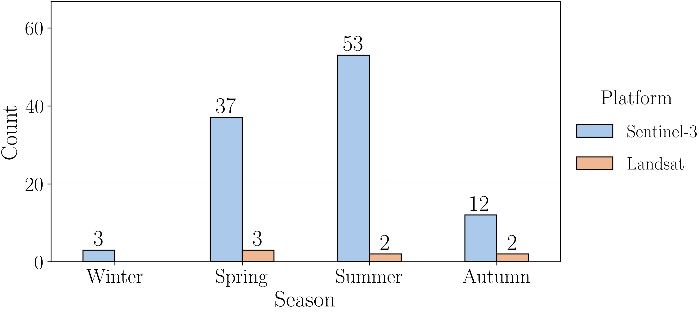
For the construction of spatio-temporal series of LST and SYN-derived indices, an automated pipeline was implemented to systematically download available imagery using OData API from Copernicus Data Space Ecosystem (CDSE) [57]. More precisely, SLSRT LST and SYN products within designated Sentinel-3 orbits that cover Denmark, clipping data to the specified Area of Interest (AOI) and assessing its cloud cover. Only images with ≤5% cloud cover in the AOI were considered in the analysis. Also, solely data collected from year 2020 to 2023 were included. This filtering resulted in a total of 112 timestamps. Because of the cloud cover fraction criterion, most of the timestamps were obtained in summer and spring ( 55 and 40 , respectively, in contrast with autumn’s 14 and winter’s 3 )—as shown in Figure 1.
Note that clouded pixels were masked out as these tend to be unfeasible as LST representatives.
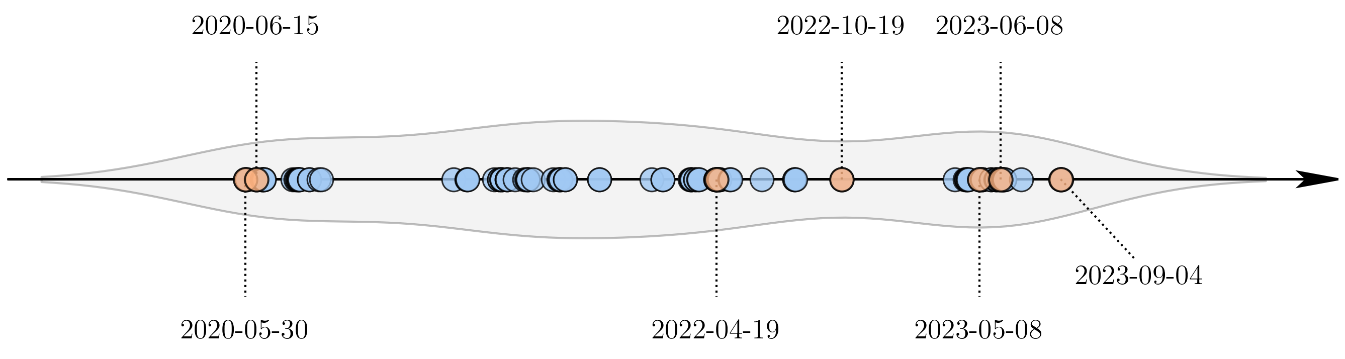
Following the assembly of the Sentinel-3 collection, an automated process identified corresponding Landsat 8/9 images within a ±30 min window of the Sentinel-3 acquisition times. This approach was designed to ensure temporal quasi-synchronisation, enhancing the matching quality of inputs for downscaling validation. Indeed, it is well known that, due to weather dynamics, the larger the time discrepancy, the smaller the correlation between the values of two sensed scenes. On the other hand, the restrictive criteria of similar sensing time and space of the native and validation remote sensing platforms combined with near-clear-sky conditions highly reduce the retrieved data that may be used for validation. A trade-off between native-validation concomitance and amount of the resultant validation data is, therefore, required. The literature reveals that a maximum time difference is usually arbitrated and with values that may be even higher than the herein proposed 30 min. Examples are the work of Li et al. [33]—33 min—Hutengs and Vohland [25]—35 min—Wang et al. [37]—43 min—and Bartkowiak et al. [48]—90 min. With the time difference threshold of 30 min, a total of 7 unique matching dates—described in Table 1, Table A1 of Appendix A.1 and Figure 1—were identified: 3 in spring, 2 in summer, 2 in autumn and none in winter. This seasonal coverage, while not comprehensive, still enables testing in different seasons, in particular, the ones when heat is a more pressing concern.
Note that the resultant matching dates pertained to each of the years between 2020 to 2023, except 2021. The timeline of all collected dates may be visualised in Figure 2.
To make the multi-timestamp models account for seasonality, year-season was considered as a possible predictor. This is a pure temporal categorical variable whose classes correspond to four meteorological groups: spring (March–April–May), summer (June–July–August), autumn (September–October–November), and winter (December–January–February).
Pure spatial variables were considered as possible predictors for all models. These refer to time-invariant geospatial predictors that describe the fixed physical characteristics of the study domain (Table 2). They provide essential information on topographic, geographic and surface-related controls that systematically modulate temperature fields and land–atmosphere interactions.
Regarding topography, Digital Elevation Models (DEMs) provide high-resolution representations of terrain height that enhance temperature modelling by explicitly accounting for elevation-dependent variability, particularly in regions with complex terrain or in proximity to coastlines and large water bodies. As noted by Oke et al. [9], such geographic controls exert a strong influence on the spatial organisation, diurnal and seasonal evolution of urban and regional thermal patterns.
To further characterise terrain-related influences, a Topographic Exposure Index (TOPEX) [58] was included to quantify spatial variations in terrain exposure and sheltering. TOPEX was computed using a Python-based workflow to ensure computational efficiency and scalability. For each grid cell in the DEM [59], terrain elevation angles were calculated along radial transects at regular distance increments (100 m) up to a maximum radius of 2 km for each directional sector. The maximum horizon (occultation) angle within each sector was retained as the TOPEX value, with positive values indicating relative topographic sheltering and negative values indicating exposure. TOPEX was computed for the eight cardinal and intercardinal directions (N, NE, E, SE, S, SW, W, NW), and a single composite index was obtained by averaging values across all directional sectors.
Proximity to large water bodies influences LST through the thermal inertia of water and associated land–sea thermal contrasts, which modulate surface heating and cooling rates. To represent this effect, Euclidean distance to the coastline (DCOAST) was computed for each grid cell using a high-resolution European coastline dataset and included as a fixed spatial predictor using QGIS (version 3.44.11) [60].
Beyond large-scale geographic controls, spatial variability in LST is also influenced by persistent surface characteristics associated with artificial surfaces, which affect radiative properties, surface moisture availability, and the partitioning of energy fluxes. Several urban-related geospatial variables were therefore included as fixed predictors. Imperviousness Degree (IMD) was used to represent the proportion of sealed surfaces within each grid cell. Impervious surfaces are associated with reduced evapotranspiration, enhanced sensible heat storage, and altered radiative behaviour, making IMD a key determinant of spatial LST variability.
Vegetation-related surface properties were also included to account for spatial differences in evaporative cooling potential. Tree Cover Density (TCD) [61] was used to represent the fraction of vegetated surfaces.
While individual surface variables describe specific physical properties, land surface temperature is often governed by the combined effect of multiple surface characteristics acting simultaneously. Local Climate Zones (LCZs) were developed to capture these combined effects by grouping areas that exhibit similar surface–atmosphere interaction behaviour under comparable atmospheric forcing. As such, LCZs provide a spatial framework for representing typical surface energy exchange regimes that emerge from the interaction of land cover, surface materials, and vegetation characteristics. The LCZ data was generated using an updated Python-based version [62] of an ArcGIS (version 10.8.2) tool developed and used in previous publications [63,64], which originally revealed an accuracy of 81%. This updated Python-based version has an agreement above 90% with the original ArcGIS tool. Rather than being introduced directly as categorical predictors, LCZ information was incorporated into the modelling framework through LCZ-specific Bowen-ratio values—here named “Urban Density” (UD)—which represent characteristic ratios between sensible and latent heat fluxes associated with different surface types [65].
To make the predictor variables suitable for modelling, data transformation was required. A consistent spatial resolution across all inputs was achieved by resampling each dataset to a common grid, using aggregation methods selected according to the characteristics of each variable. Specifically, predictor values were summarised within a regular 0.002 × 0.002° grid through zonal statistics. This procedure, implemented in QGIS [60], calculates descriptive statistics for each grid cell—such as mean, median, sum, minimum, maximum, majority, or range. Unlike simple point-based sampling at cell centroids, zonal statistics reduce the likelihood of assigning non-representative extreme values, as they account for all pixels within each target cell. Consequently, the statistical measure applied to each predictor depended on its data type, with different approaches used for continuous and categorical variables, as summarised in Table 2.
Table 2. Final predictor data sources and corresponding zonal statistics methods for resampling to the regular 0.002 × 0.002° grid.
PredictorSource and ReferencesZonal Statistic Method
Digital Elevation Model (DEM)EU-DEM (30 m resolution) from Eurostat [66]Mean
Topographic Exposure Index (TOPEX)In-house Python tool (30 m of resolution) based on the works of Oliveira et al. (2021) [18] and Chapman (2000) [58]
Distance to the Coast (DCOAST)QGIS ( 0.002 of resolution ( 220 m × 120 m)) [60]
Imperviousness Density (IMD)Imperviousness density (2018; 10 m resolution) from Copernicus Land Monitoring Service [67]
Tree Cover Density (TCD)Tree cover density (2018; 10 m resolution) from Copernicus Land Monitoring Service [61]
Local Climate Zones in Bowen Ratio (UD)In-house Python tool (50 m resolution) based on the works of Oke et al. (2017) [9], Oliveira et al. (2021) [68] and Stewart and Oke (2012) [69]Majority

2.1.2. Data Splitting and Training/Validation/Testing Strategy

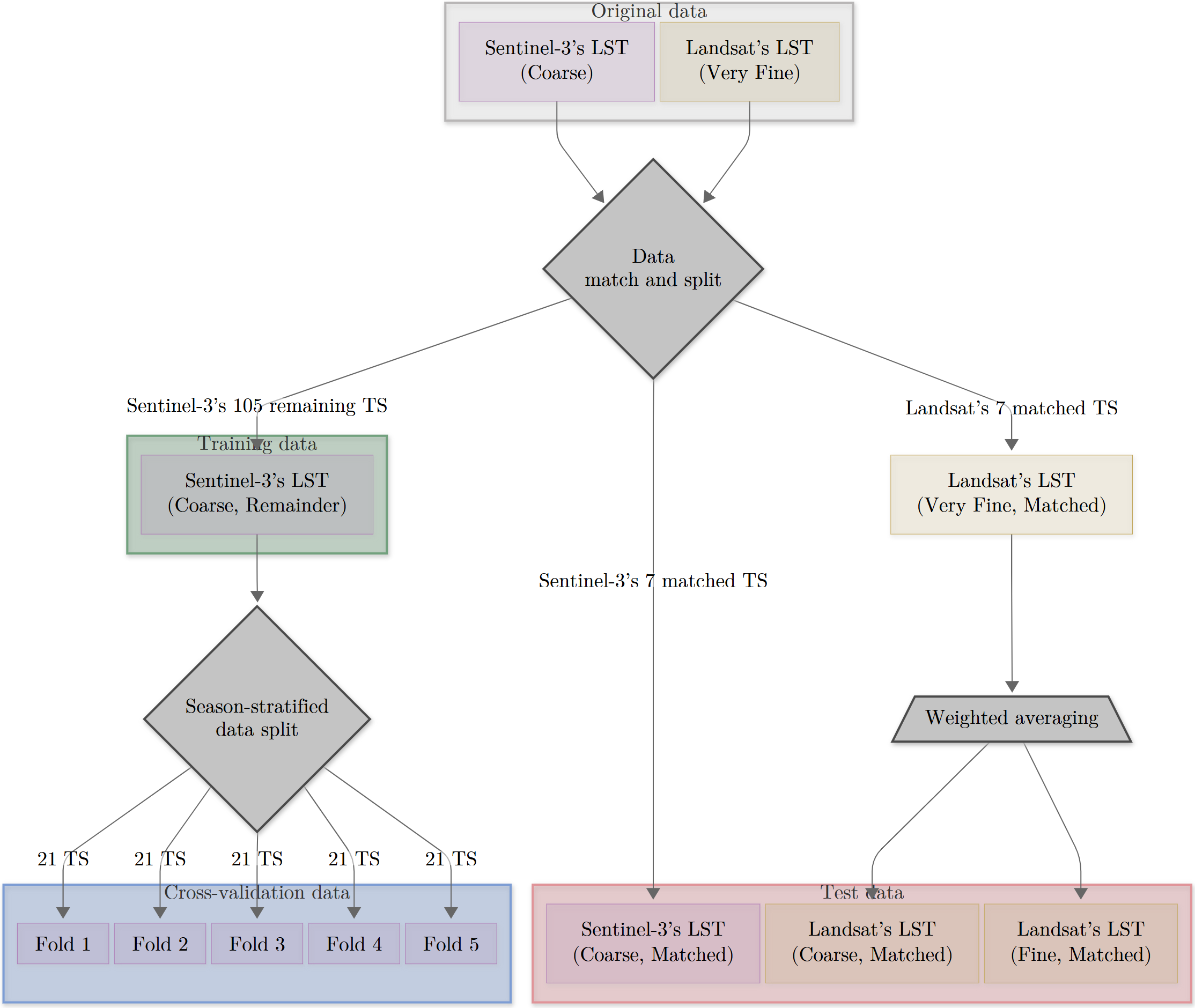
Sentinel-3’s 7 timestamps for which there were fine Landsat matched data were considered for testing (see Table 1). With them, it was decided to define three different kinds of tests: two for coarse and fine predictions using Landsat LST data reprojected to Sentinel-3’s fine and coarse grids (these grids are associated with OLCI and SLSTR sensors, respectively) and one for coarse prediction using Sentinel-3’s LST . The purpose of considering a coarse test using Landsat data, besides another using Sentinel’s, was to assess how the two datasets differed in a common coarse grid and if such differences could influence the results in the fine test. Differences could indeed arise due to multiple factors such as lack of synchronicity in the acquisitions, different view angles, and LST computation algorithms.
The conception of the downscaling models would require hyperparameter tuning and subsequent training, besides testing. It was decided to perform the hyperparameter tuning by picking the remaining 105 timestamps and doing a 5-fold cross-validation scheme stratified by season. In practice, this means that each fold contained approximately the same proportion of data for each season as in the original data. In this way, the performance of the models is proportionally assessed with respect to seasonality. In such hyperparameter tuning, for each candidate set of hyperparameter values, the models were trained with 4 folds and validated with 1 , further rotating the validating fold until all of them were used. The resulting cross-validation scores were then defined as the arithmetic mean of the respective validation scores. And the set of hyperparameter values with the highest cross-validation score was the one taken. With tuning done, the models were retrained using the whole cross-validation data and subsequently tested on the test subset (i.e., the withheld Landsat–Sentinel pairs mentioned in Table 1).
The whole data architecture considered in this work is summarised in Figure 3.

2.2. Methods

2.2.1. Hypothesis of Scale Invariance

Scale invariance [70,71,72] corresponds to the conservation of relation between variables with respect to scale, or in practical terms, to grids of different resolution. Let f be the relation between predictors X and target LST . And let “coarse” and “fine” denote grids of coarse and fine resolution, respectively. Under the assumption of scale invariance, the relationship between land surface temperature and its predictors can be expressed as LST coarse = f X coarse and LST fine = f X fine . This hypothesis was taken in the present work by training the base model f with predictors and target on Sentinel-3’s coarse grid ( X coarse and LST coarse ) and inferring LST fine through f using predictors on Sentinel-3’s fine grid ( X fine ) as a first approximation.
It is important to exercise caution when assuming that a relation f is scale-invariant. It is well known that scale invariance does not hold in all cases [73,74]. For instance, if the coarse data are regarded as a weighted average of the fine data, scale invariance from a finer to a coarser grid would mean conservation of the relationship with respect to averaging. However, averaging tends to shrink the distribution of values which may cause relationships observed at the coarse grid to break at fine-scale extremes.

2.2.2. Residual Correction

Given the true Sentinel-3 coarse resolution values, LST coarse , and the ones predicted by the trained model f , LST ^ coarse , the coarse-scale prediction residual ( ε coarse ) can be computed as
ε coarse = LST coarse LST ^ coarse ,
and used to estimate the fine prediction residual ( ε fine ). In this work, the fine-resolution prediction residual was approximated by interpolation of the coarse prediction one onto the fine grid, that is,
ε fine = LST fine LST ^ fine interp fine ε coarse = : ε ^ fine .
Such an approximation would be exact, for example, if the true LST fine was an interpolation of the true LST coarse and if the predicted LST ^ fine was obtained by an interpolation of LST ^ coarse instead of the application of the model f on the fine predictors.
Given the estimated fine-scale prediction residual, it is then possible to correct the LST ^ fine values predicted by f through
LST ^ fine , corr = LST ^ fine + ε ^ fine .
This procedure is called “residual correction” [75].
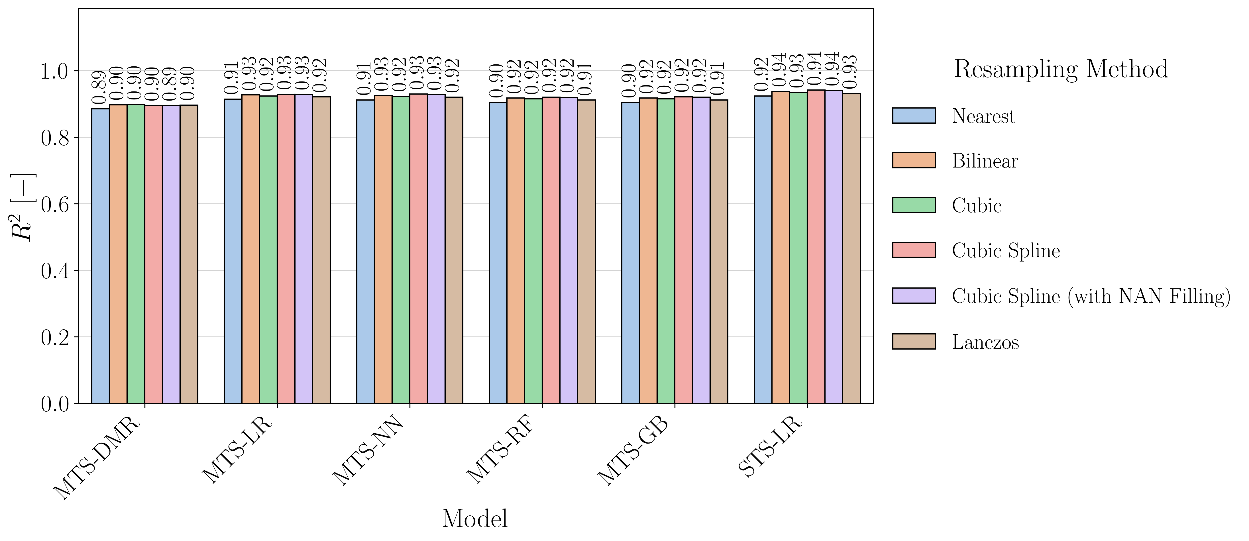
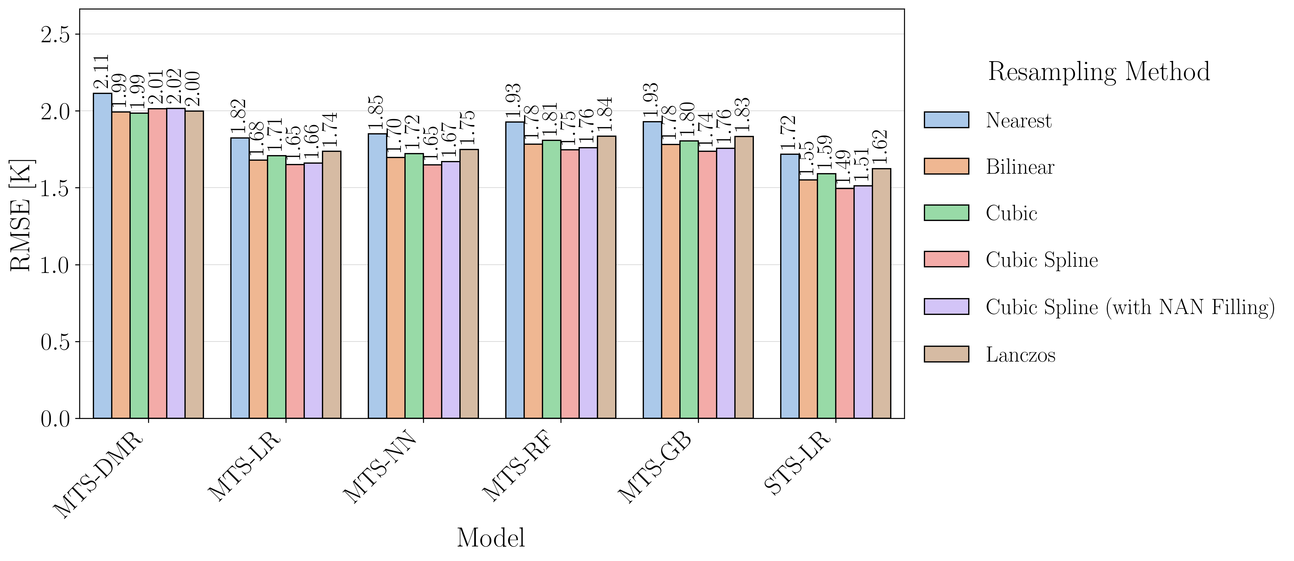
One should note that many different interpolation methods may be considered in resampling of the coarse residuals. The literature had revealed bilinear and cubic interpolation to be commonly used in the refinement of remotely sensed numerical variables [76]. In the present work, these and also nearest-neighbour, cubic spline and Laczos interpolation methods (provided by rasterio Python package [77]) were tried and the obtained test scores are presented in Figure A17, Figure A18, Figure A19, Figure A20, Figure A21 and Figure A22 of Appendix A.3. Although the figures evidence cubic spline to be the best performer followed by bilinear interpolation, cubic spline interpolation requires a larger number of neighbouring points, and, because of this, it significantly propagates missing values of the bounding water bodies inland. For this reason, cubic spline interpolation was considered together with missing value-filling using the result from bilinear interpolation. The above-mentioned figures show that this method does perform better than pure bilinear interpolation.

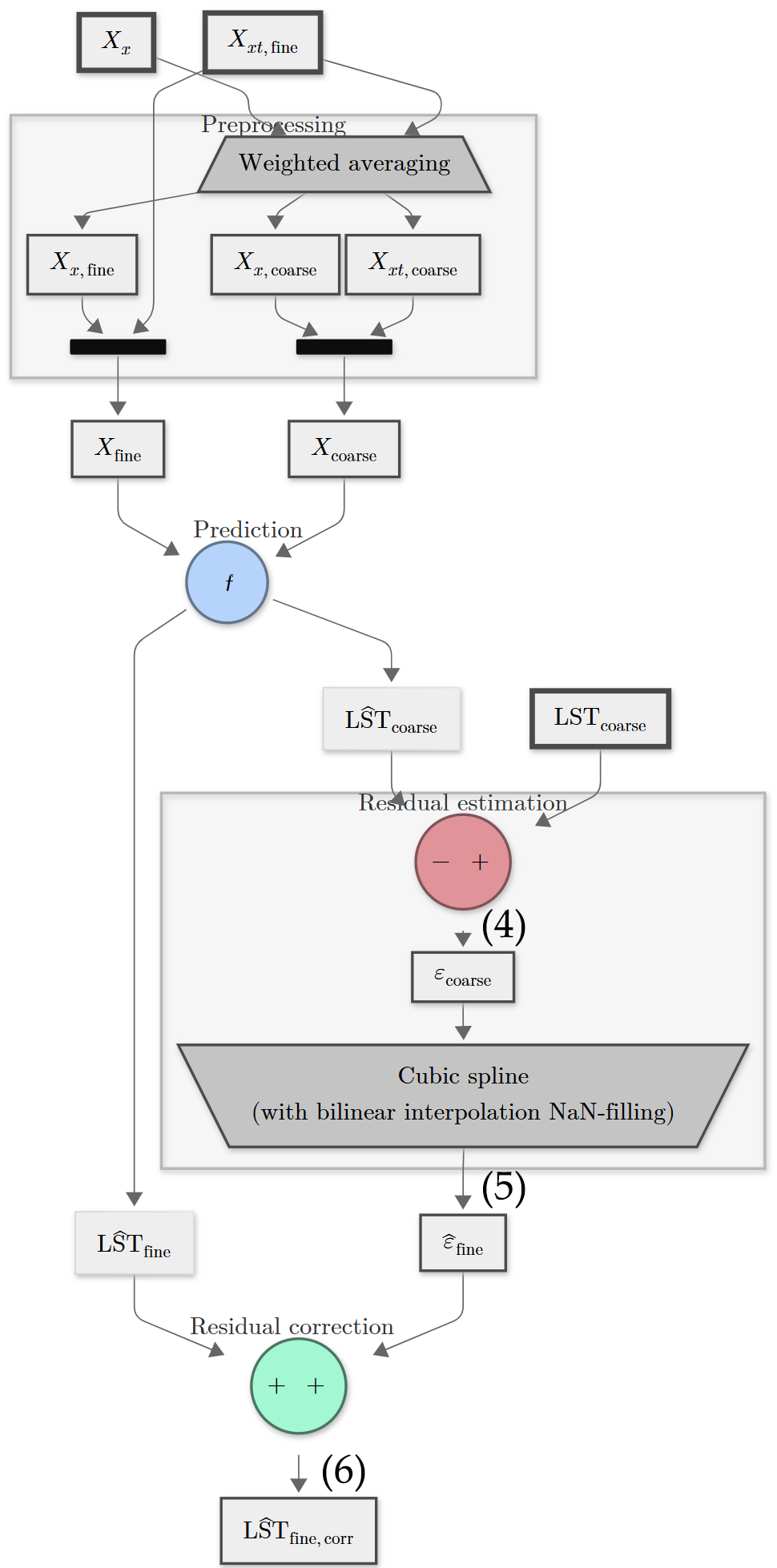
2.2.3. Architecture of the Single-Timestamp Model (STS)

Figure 4 presents the architecture of the single-timestamp model considered in this work, which is based on the scale invariance principle and subsequent application of residual correction. In this architecture, and as mentioned before, the base model f is trained with coarse predictors ( X coarse ) and coarse LST ( LST coarse ). It predicts a coarse LST ( LST ^ coarse ) or fine one ( LST ^ fine ) whether the issued predictors are coarse ( X coarse ) or fine ( X fine ). The coarse predictors correspond to spatio-temporal and pure spatial predictors aggregated over Sentinel-3’s coarse grid ( X x t , coarse and X x , coarse , respectively). Similarly, the fine predictors correspond to a combination of the original spatio-temporal predictors ( X x t , fine ) and the very fine pure spatial predictors aggregated over Sentinel-3’s fine grid ( X x , fine ). Weighted averaging was herein employed as an aggregation method, where the value assigned to a fine pixel is computed as the average of all overlapping coarse-pixel values weighted by their respective overlap areas. This method has been regarded appropriate for the coarsening of raster data [78] and has been widely used in the literature. Examples of works that employed weighted averaging in a manner similar to the present manuscript’s are the ones by Agam et al. [32], Mukherjee et al. [79], Dominguez et al. [80], Gao et al. [81], Sánchez et al. [75], Bartkowiak et al. [48], Lie et al. [47] and Wang et al. [43].
The predicted fine LST ( LST ^ fine ) is then corrected using the estimation (5) for the fine residual ( ε ^ fine ). This architecture has been shown to be quite effective in the prediction of fine LST using a base model trained with coarse data from the very same timestamp [32,37,42]—hence the designation “single-timestamp model”.

2.2.4. Architecture of the Multi-Timestamp (MTS) Model

There are several downsides of using a pure timestamp-specific model when compared to a general (multi-timestamp) one. The training data is quite limited—it solely concerns the coarse data of the timestamp whose fine target is to be inferred. The coarse data of the timestamp does not necessarily fully describe the respective fine data. For instance, when one obtains coarse data through weighted averaging of the fine data, the tails of the value distribution diminish, and some of the information is inevitably lost. Information may be added by considering coarse data from multiple other timestamps. The central question is whether the additional information is consistent with the fine-resolution data of the target timestamp. It should also be noted that considering single-timestamp ML models beyond LR would be rather impractical. Not only do ML models usually require larger amounts of data in their training (so that they become general enough, avoiding overfitting) but their hyperparameters must also be tuned. Performing such tuning for each timestamp would be infeasible: the already few coarse data of a sole timestamp would need to be batched into different folds for cross-validation or early stopping, the results could be too biased, and the task would need to be repeated for every single timestamp. A more convenient approach is to conceive a multi-timestamp ML model, tune and train it with coarse data from several timestamps, enabling inference for new ones without the need for further hyperparameter retuning and retraining. Note that the authors do acknowledge that single-timestamp architectures using ML base models have been widely reported in the literature, but a higher interest in operationality would inevitably imply discarding such option.
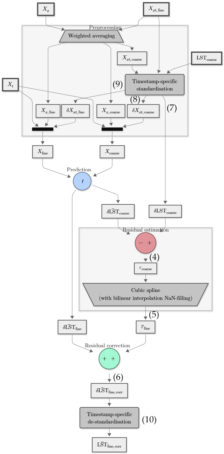
As it will be shown later in the Section 3, timestamp-specific standardisation of the target in a multi-timestamp architecture is highly recommended since, in contrast with the raw default case, it better conserves the strong predictor–target correlation in each timestamp. The multi-timestamp model with timestamp-specific standardisation can be further extended by incorporating spatio-temporal ( X x t ), purely spatial ( X x ) and purely temporal ( X t ) predictors. The flowchart of Figure 5 describes this general architecture. In this architecture, the base model f is trained with coarse predictors ( X coarse ) and standardised coarse LST ( δ LST coarse ). Therefore, it predicts a standardised coarse LST ( δ LST ^ coarse ) or a fine one ( δ LST ^ fine ) whether the issued predictors are coarse ( X coarse ) or fine ( X fine ). The coarse predictors correspond to pure temporal predictors ( X t ), standardised coarse spatio-temporal predictors ( δ X x t , coarse ) and coarse pure spatial predictors ( X x , coarse ). The standardised coarse spatio-temporal variables are obtained from the raw ones through
δ LST coarse = LST coarse LST - coarse s LST coarse ,
δ X x t , coarse = X x t , coarse X ¯ x t , coarse s X x t , coarse ,
where s LST coarse , s X x t , coarse , LST - coarse and X ¯ x t , coarse correspond to the sample standard deviations and arithmetic means of the coarse LST and spatio-temporal predictors associated with the given timestamp.
Similarly, the fine predictors correspond to a combination of pure temporal variables ( X t ), standardised fine spatio-temporal predictors ( δ X x t , fine ) and fine pure spatial predictors ( X x , fine ). Note that since the base model f is trained with standardised coarse spatio-temporal predictors, the fine ones are expected to be standardised using the coarse statistics as well, that is,
δ X x t , fine = X x t , fine X ¯ x t , coarse s X x t , coarse .
The predicted standardised fine LST ( δ LST ^ fine ) is corrected using an estimation for the fine residual ( ε ^ fine ). As previously mentioned, this estimation is simply an interpolation of the coarse residual ( ε coarse ) onto the fine grid, and the coarse residual is in turn the difference between standardised coarse LST ( δ LST coarse ) and the predicted standardised coarse LST ( δ LST ^ coarse ). The corrected predicted standardised fine LST ( δ LST ^ fine , corr ) must be then de-standardised. The process of de-standardisation for obtaining the actual corrected fine LST also involves the coarse statistics:
LST ^ fine , corr = s LST coarse δ LST ^ fine , corr + LST - coarse .
In contrast with the single-timestamp architecture, the base model f of the multi-timestamp architecture is trained with combined coarse data from multiple timestamps. It predicts a standardised LST instead of a raw one. And the regarded spatio-temporal predictors are also standardised. In both architectures, f is pixel-agnostic, or, in other words, value-specific, that is, it is a function that does not depend on space but purely on the values of the predictors in that space. There is then one and only one function f for all pixels. This means that the positioning of the variable values in the pixel matrix is irrelevant to f . The predictor and target values in a pixel constitute a single observation, and the training dataset associated with a single timestamp becomes a collection of such observations, regardless of their position. And the training dataset associated with multiple timestamps naturally corresponds to a concatenation of the data collections of the multiple timestamps.

2.2.5. Candidate Base Models

Besides LR, three different ML models were considered as possible candidates for the base model f of the multi-timestamp downscaling architecture: Feed-Forward Neural Network (MLPRegressor from scikit-learn [82]), Random Forest and Gradient Tree Boosting (XGBRFRegressor and XGBRegressor, respectively, from XGBoost [83]). For further benchmarking, the Dummy Mean Regression (DMR) model (from scikit-learn [82]) was also considered. Note that DMR always predicts the arithmetic mean of the target values seen in training, and one may show that, when considering residual correction, the resulting downscaling model is equivalent to pure interpolation of the true coarse Sentinel-3’s LST onto Sentinel-3’s fine grid. In fact, this is true for any scale-invariance-based downscaling architecture with a base model f that predicts a constant c and uses a linear operating interpolation method (that is, an interpolation method that satisfies the properties of a linear operator, namely addition and scaling) for residual refinement (see proof (A4) provided in Appendix A.2).

3. Results

3.1. Exploratory Data Analysis

3.1.1. Area of Interest and Its Local Climate Zones

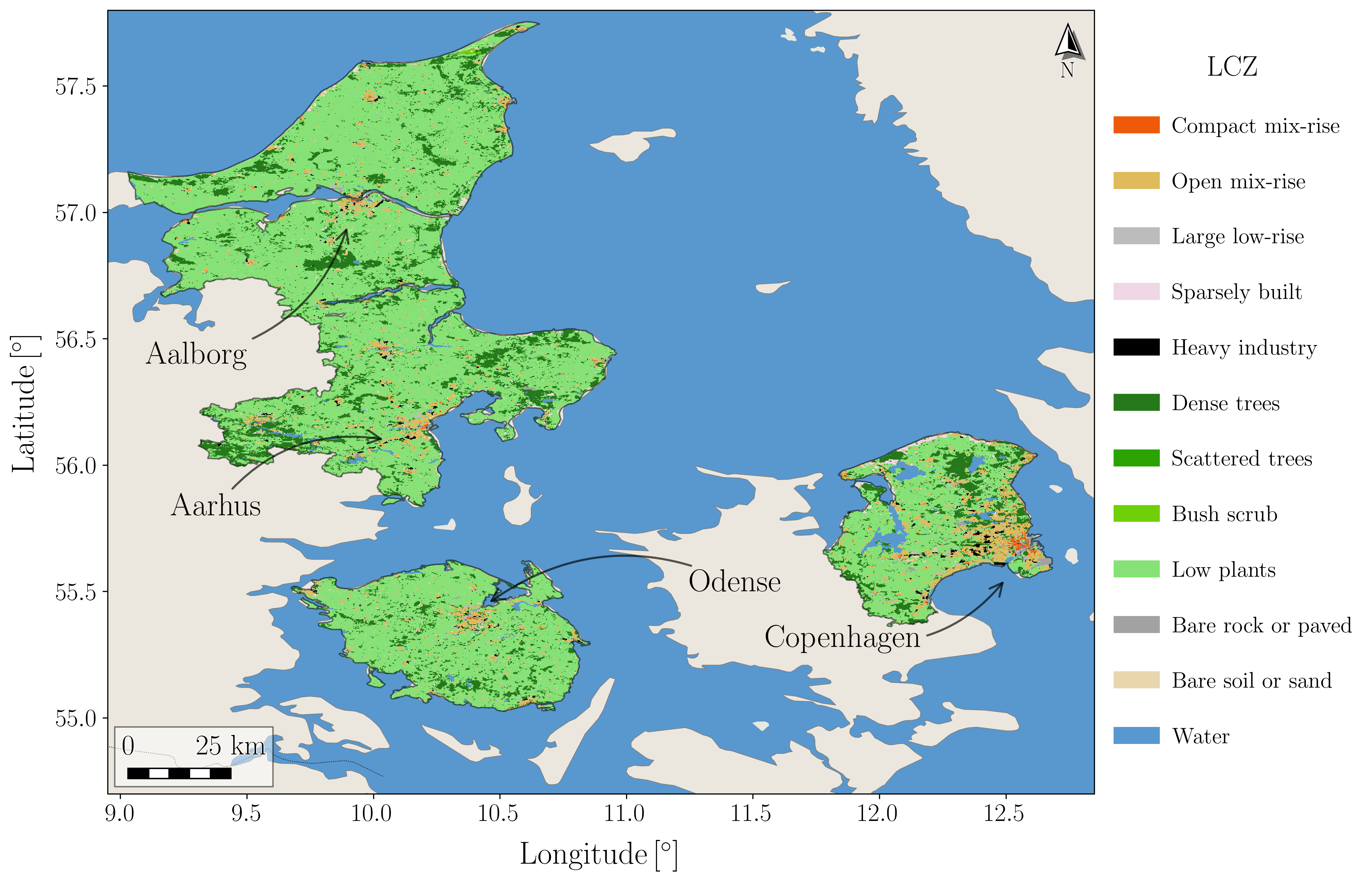
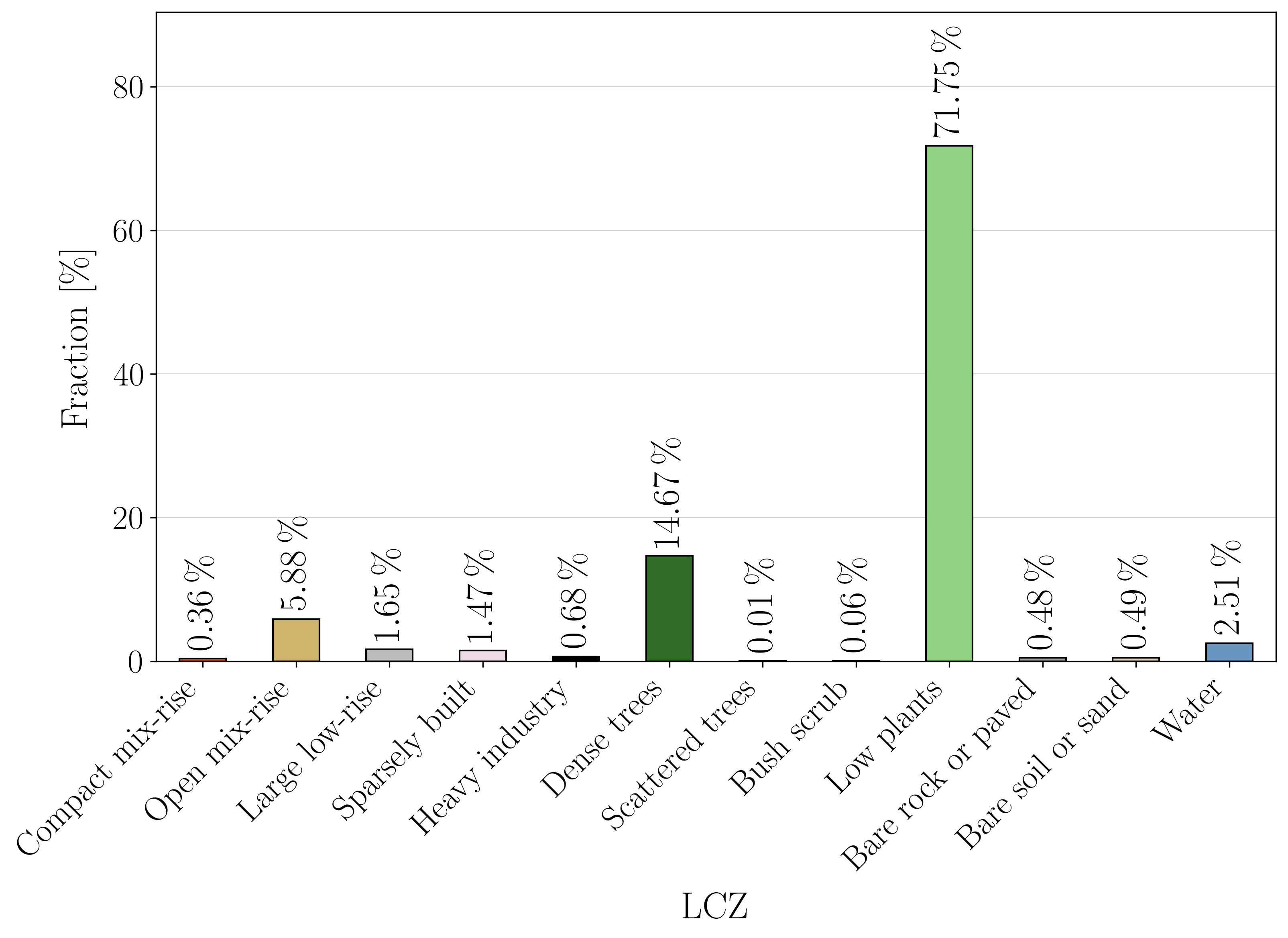
The Area of Interest (AOI) of the present work in the common geospatial predictor grid (having resolution 0.002 ) and the respective Local Climate Zones (LCZs) are described in Figure 6. Furthermore, the percentage frequency distribution of these local climate zones is presented in Figure 7. The figures reveal that the AOI mostly comprises low plant areas ( 72 %) followed by dense trees ( 15 %), open mix-rise (openly arranged buildings within low plant and scattered tree areas) ( 6 %), water ( 3 %), large low-rise (openly arranged large low-rise buildings within paved soil) ( 2 %), sparsely built (sparse arrangement of buildings in a natural setting) ( 1 %) and heavy industry ( 1 %). The remainder (bare soil or sand, bare rock or paved, compact mix-rise (dense mix of buildings within paved soil), bush scrub and scattered trees) are trace local climate zones and sum to approximately 1 %. The Danish FUAs are, therefore, much more represented by highly vegetated areas than built-up ones.

3.1.2. Correlation Between Variables

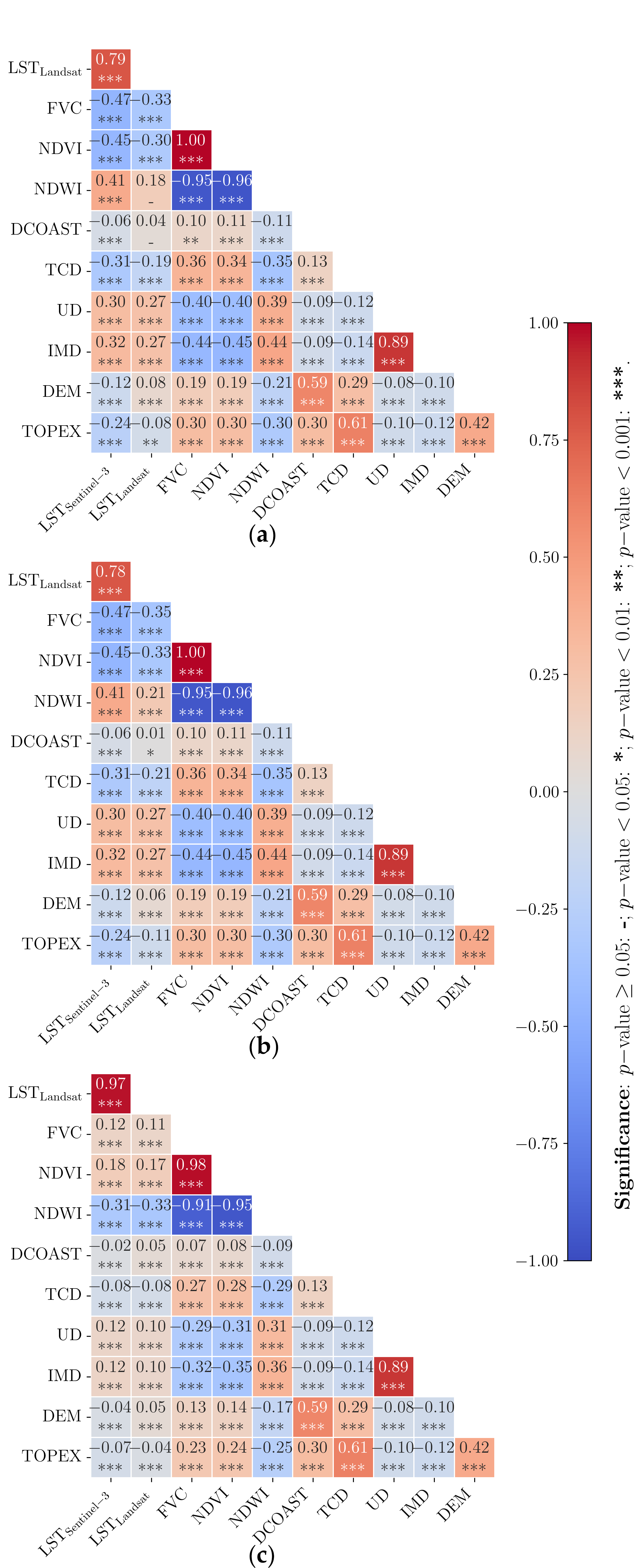
Figure 8a presents the arithmetic mean of the Pearson correlation matrix of the numerical coarse data for each test timestamp. It reveals that Sentinel-3 and Landsat LST data do differ, having a correlation coefficient corresponding to 0.79. One should be aware that this could possibly introduce some bias when comparing the downscaling results of the different models with the fine Landsat data. Furthermore, if one assumed that the relation between coarse Sentinel-3 and Landsat data coincided with that between downscaled Sentinel-3 and fine Landsat data, a coefficient of determination of solely R 2 0.62 would be (on average) expected.
Figure 8a also shows that the predictors that have the highest (in absolute value) correlation coefficient with respect to Sentinel-3’s LST corresponded to the spatio-temporal ones: FVC ( 0.47 ), immediately followed by NDVI ( 0.45 )—which is almost collinear with FVC—and NDWI ( 0.41 )—which is also highly correlated with the other two. Predictors with a smaller but moderate correlation coefficient corresponded to IMD ( 0.32 ), TCD ( 0.31 ), UD ( 0.30 )—which is highly correlated with IMD—and TOPEX ( 0.24 )—which is significantly correlated with TCD. Other not so correlated predictors corresponded to DEM ( 0.12 ) and DCOAST ( 0.06 )—which is significantly correlated with the former. Figure 8c further presents the Pearson correlation matrix that is obtained when considering the coarse data combined. By comparing it against the arithmetic mean of Pearson correlation matrices for each timestamp, one finds that all correlation coefficients between predictors and Sentinel-3’s LST significantly decrease (in absolute value) when considering data combination. The change in the values of the correlation coefficients is particularly pronounced for the predictors that originally showed the strongest correlation values (i.e., FVC , NDVI and NDWI )—the values not only diminish but also exhibit sign reversal. This may be explained by the fact of FVC , NDVI and NDWI not corresponding to actual physical quantities but normalised indexes ( FVC is within the range 0 , 1 , NDVI and NDWI are within 1 , 1 ). Although within a given same timestamp it is uncommon to have largely different LST values associated with the same FVC , NDVI or NDWI values, this relationship does not persist across different timestamps, and linearity is, therefore, reduced.
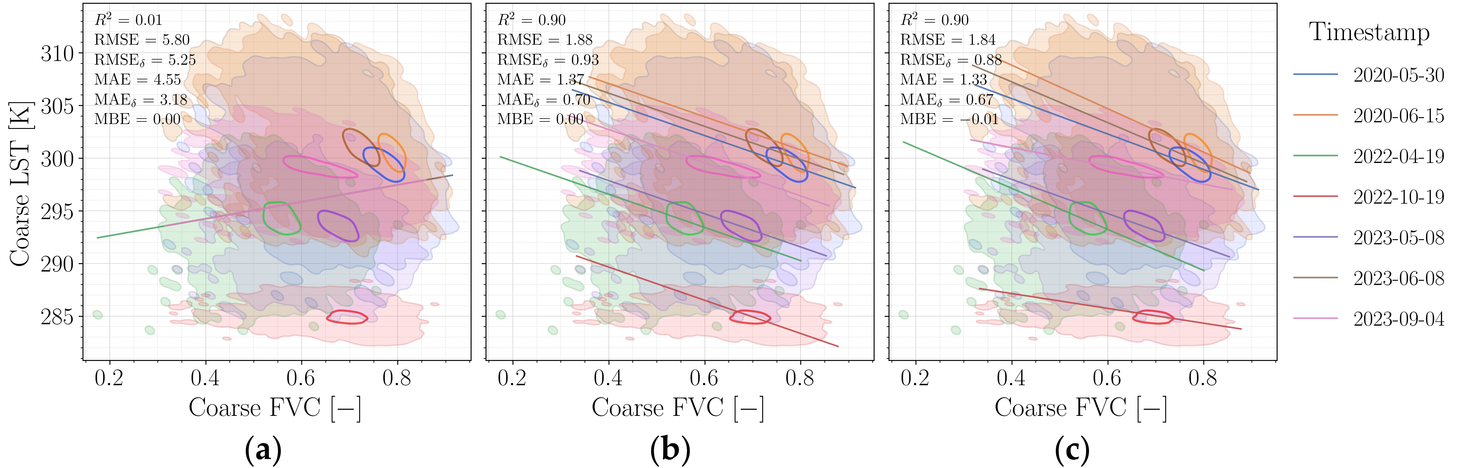
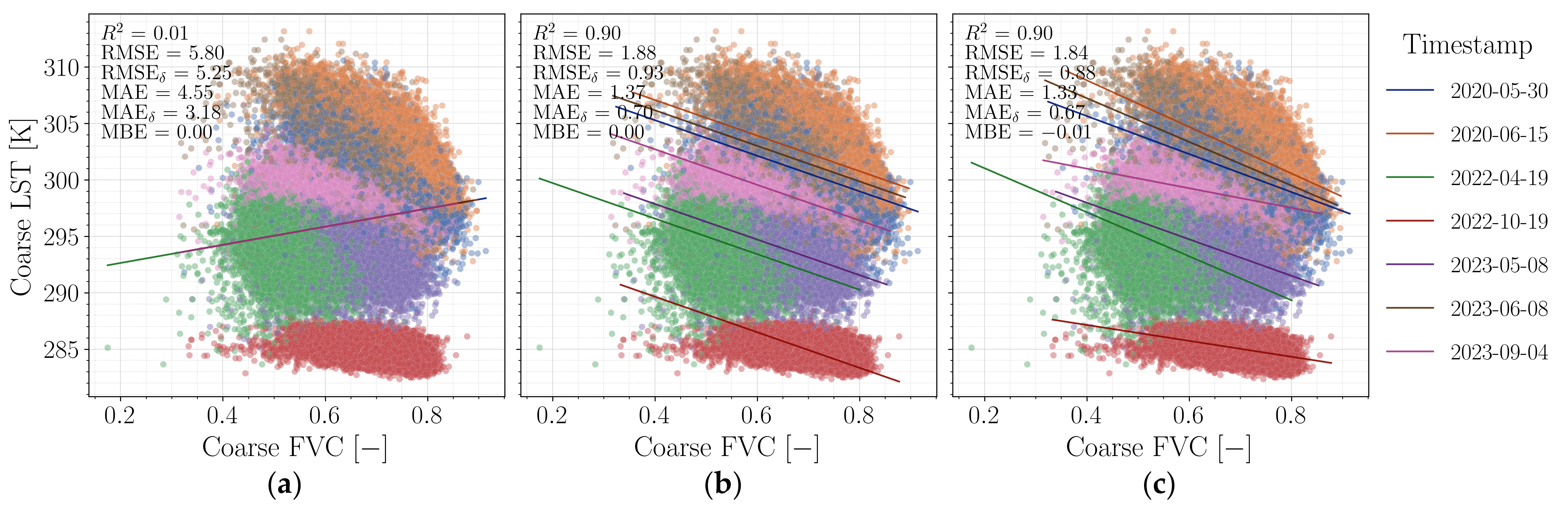
Figure 9 shows how significantly distinct Sentinel-3 LST values from different timestamps can correspond to the same FVC value. It also shows for each timestamp alone an approximate linear relationship between LST and FVC . Therefore, in the absence of data transformations, a single-timestamp LR model would be expected to perform with higher accuracy than a multi-timestamp one. The straight line in Figure 9a, corresponds to the predicted LST using a multi-timestamp LR model with FVC as a predictor. This line does not agree with the actual data and can only roughly estimate the overall average, producing an R 2 value of just 0.01 . The figure further shows that the data of each timestamp mostly differs in offset. This suggests that a multi-timestamp model based on centred variables (raw variables with their timestamp-specific means subtracted) may perform better than one on the raw variables. When using (A1) (see Appendix A.2) as model and training it with the combined coarse data of the test timestamps, the result presented by Figure 9b, is obtained. The R 2 score abruptly increases from 0.02 to 0.90 , the Root Mean Square Error ( RMSE ) decreases from 5.80 to 1.88 K and the predicted LST lines much better agree with the actual data.
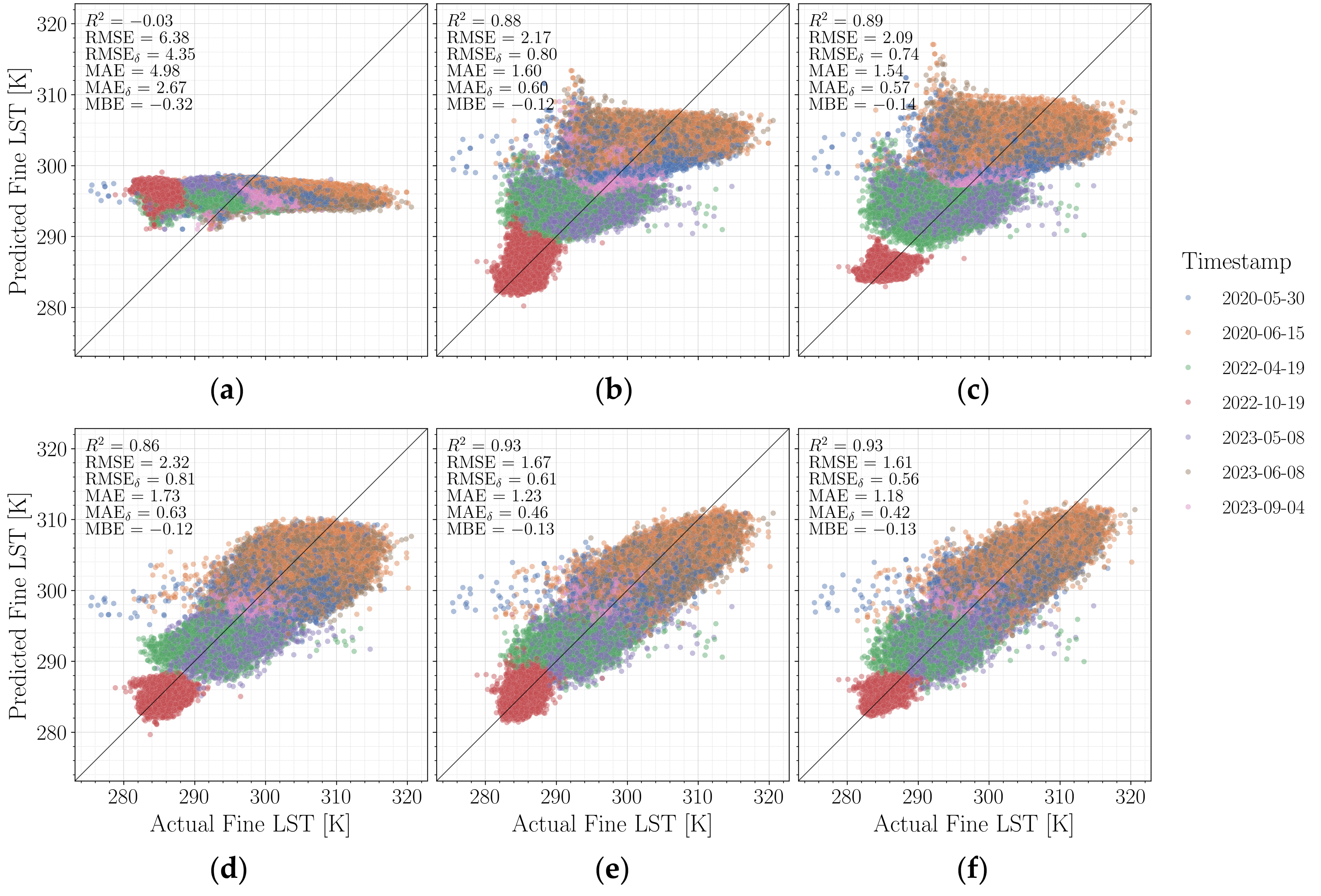
Note how, in Figure 9b, all the predicted L S T lines not only have their own distinct offset but a common slope whereas the actual data shows some slope variance. A reasonable approximation for the slope of the actual data for timestamp t could be defined as s LST t / s FVC t , where s LST t and s FVC t are the sample standard deviations of the L S T and F V C values for timestamp t . The exact slopes may be approximately achieved by considering timestamp-specific standardisation of the variables (division of the centred variables by the timestamp-specific sample standard deviations of the respective raw ones) instead of centring. With the timestamp-specific standardisation LR model (A2) (see Appendix A.2) trained with the coarse data of all test timestamps, the right-hand side subplot in Figure 9c, is obtained. The resultant metrics improve just marginally, with R M S E decreasing by solely 0.04   K . It would also be important to know how standardisation may improve fine-prediction performance. Figure 10 shows that with standardisation, fine-prediction R M S E decreases from 2.17 to 2.09 K (that is, by 0.08 K ) when disregarding residual correction and from 1.67 K to 1.61 K (that is, by 0.06 K ) when regarding it. Although the improvements are still small, they are not completely insignificant, motivating the implementation of timestamp-specific standardisation.
It is important to note how Figure 10 shows that residual correction is highly effective in the reduction of the downscaling error: for the case of standardisation, it diminishes RMSE by as much as 0.48   K ( 23 %).
The similarity between the single and multi-timestamp LR models when considering timestamp-specific standardisation of the spatio-temporal variables while using a single predictor is further highlighted by the close agreement between the resulting Pearson correlation matrices, shown in Figure 8a,b, respectively. The curious reader may access Appendix A.2 to understand how such proximity may be mathematically justified.
The current results justified the usage of timestamp-specific standardisation in a multi-timestamp downscaling model.

3.2. Hyperparameter Tuning

3.2.1. Selection of Numerical Predictors for a Multi-Timestamp Linear Regression Model

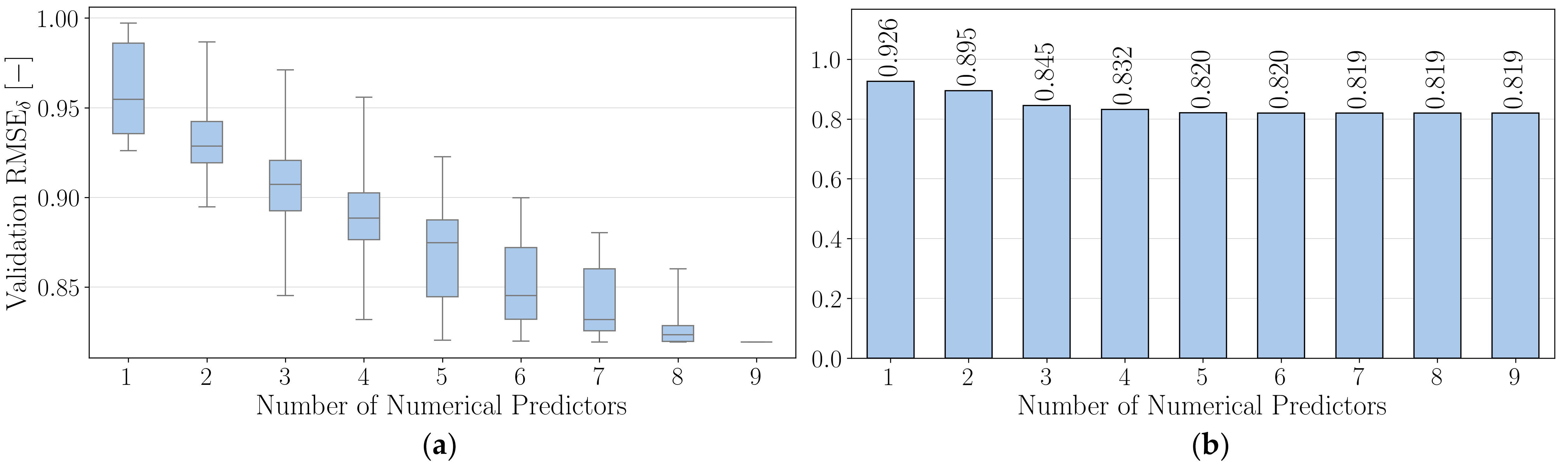
The numerical predictors for a multi-timestamp LR model may be selected as the combination that yields the highest cross-validation score. There are nine possible numerical predictors: FVC , NDVI , NDWI , IMD , TCD , DEM , TOPEX, UD and DCOAST. This results in 2 9 1 = 511 possible combinations. Figure 11 shows the obtained cross-validation RMSE values for the predicted standardised coarse target ( RMSE δ ) for each number of numerical predictors—as a distribution (at the left-hand side, (a)) and as the best value (at the right-hand side, (b)) for each number. As expected, and overall, the RMSE δ values tend to decrease with the number of numerical predictors. When examining the best-performing models for each predictor count, one finds the RMSE δ values to swiftly decrease with number of predictors but then to stagnate from five to nine.
Table 3 presents the best combinations of predictors for each of their numbers sorted from worst to best. By defining the best compromising overall combination as the set with the smallest number of predictors that achieves the lowest RMSE δ value to the second decimal place, the combination FVC , IMD , NDWI , TCD and DCOAST (five predictors) is obtained. The other predictors— DEM , TOPEX , UD and NDVI —were ultimately found to be of lesser importance. This could be explained by the strong correlation of these with the predictors already included in the set of five. Indeed, and as shown in Figure 8b, DEM is highly correlated with DCOAST, TOPEX with TCD , UD with IMD , and NDVI with FVC and NDWI .
The present result shows how inter-correlation may make the best set of predictors differ from the one that would be obtained if singular predictor–target correlations were considered. For instance, as shown by Figure 8b, if the predictors were not correlated between themselves, one would expect DCOAST to be the least important variable, achieving the ninth place. However, the current study reveals it to be the fifth most important one. And this may be explained by the fact of all the others, in contrast with DCOAST , being much more correlated with the most important predictor, FVC , which means that a substantial part of their information is already present in this variable, thus not adding more than the poorly   FVC -correlated DCOAST variable.

3.2.2. Selection of Categorical Predictors for a Multi-Timestamp Linear Regression Model

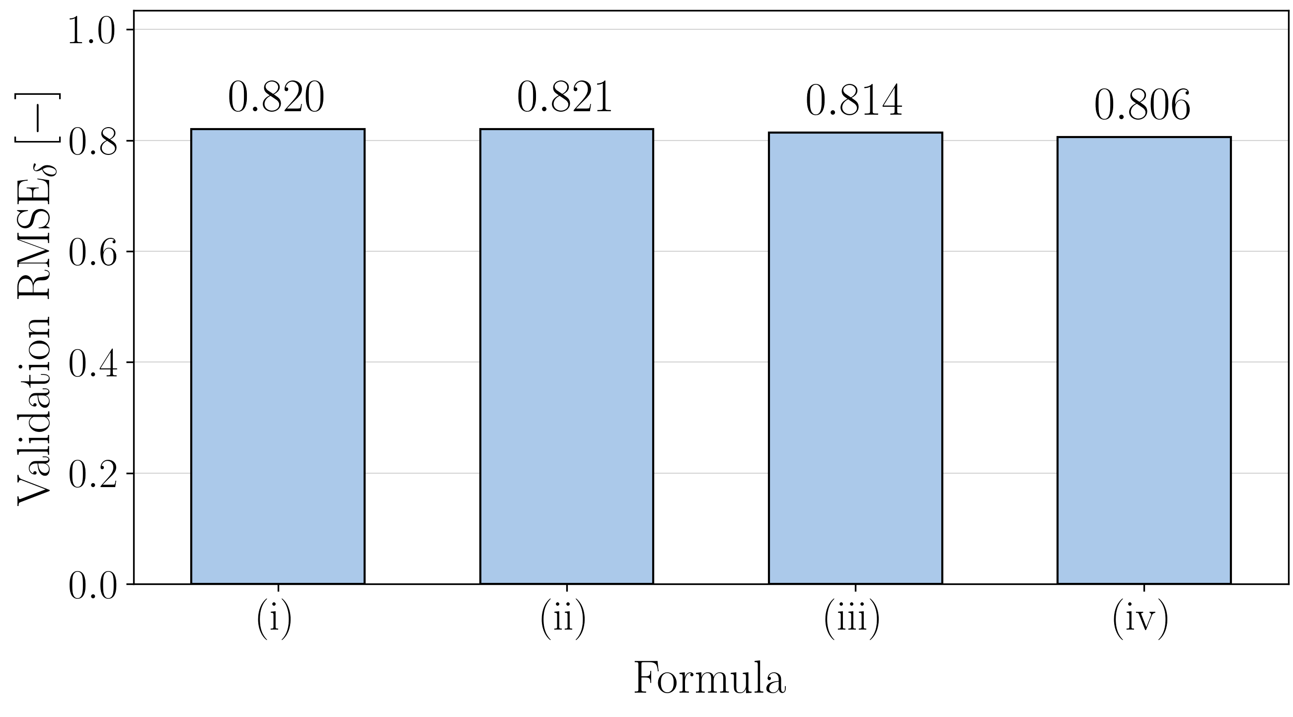
To incorporate seasonal effects in the multi-timestamp LR model, season was considered as a potential predictor in addition to the most relevant numerical variables identified in the previous section. Season is a categorical variable whose inclusion in a linear model may be done in different ways. Four linear model configurations were tested: (i) a model with no seasonal dependence; (ii) a model with season-specific intercepts; (iii) a model with season-specific intercepts and slopes applied exclusively to the spatio-temporal predictors ( FVC and NDWI ); and (iv) a model with season-specific intercepts and slopes applied to all numerical predictors. All these models may be conveniently expressed through so-called Wilkinson formulas [84]:
( i ) :   LST FVC   +   IMD + NDWI   +   TCD   +   DCOAST ,
( ii ) :   LST Season + FVC + IMD + NDWI + TCD + DCOAST ,
( iii ) :   LST FVC + NDWI Season + IMD + TCD + DCOAST ,
( iv ) :   LST FVC + IMD + NDWI + TCD + DCOAST Season .
Note that season-specific intercepts and slopes are such that, in the occurrence of some season, the linear model parameters that are associated with any other are disregarded.
Similarly to what was done in the tuning of numerical predictors, the four different formulas were cross-validated, and the best one was defined as the simplest formula yielding the smallest RMSE δ value to the second decimal place. Figure 12 shows how the increasing complexity of the formulas did result in lower RMSE δ values. By rounding RMSE δ to two decimal places, the formula with season-specific intercepts and slopes applied to all spatio-temporal numerical predictors (iii) was found to be the best configuration.
  • Hyperparameter Tuning of Multi-Timestamp ML Models
As mentioned before, three different ML models were considered as possible candidates for the base f of the multi-timestamp downscaling architecture: NN, RF and GB. In the case of these models, all predictors except NDVI (which is almost collinear with FVC ) were considered. The hyperparameters were tuned using Optuna [85] based on the cross-validated RMSE δ score.
In all ML models, the method considered in the scaling of the numerical predictors—standardisation or min–max normalisation—was regarded as a tunable hyperparameter. In the setting of the NN architecture for tuning, the following specifications were considered: dummy encoding (that is, one-hot encoding with the drop of one of the resultant components to remove redundancy) of the categorical predictors (Season), Rectified Linear Unit (ReLU) activation functions and training with Adaptive Moment Estimation (ADAM) gradient descent using mini-batches of size 1024 , with a maximum number of 1000 epochs. One also considered early stopping with 20 % of the data for validation using R 2 as scorer, a patience of 10 epochs and tolerance of 0.001 in the validation score.
Table 4 shows the obtained tuned values for some of the notable hyperparameters of the three ML models.
A note should be made regarding the encoding of Season in the tree-based models: the choice between dummy encoding and optimal partitioning [86] was treated as a tunable hyperparameter. In the case of optimal partitioning, splits are optimally done with respect to groups of categories (more specifically, the indicator of the occurring category belonging to that group) instead of to a category alone (more specifically, the indicator of the occurring category corresponding to that one).

3.3. Training, Cross-Validation and Test Overall Scores

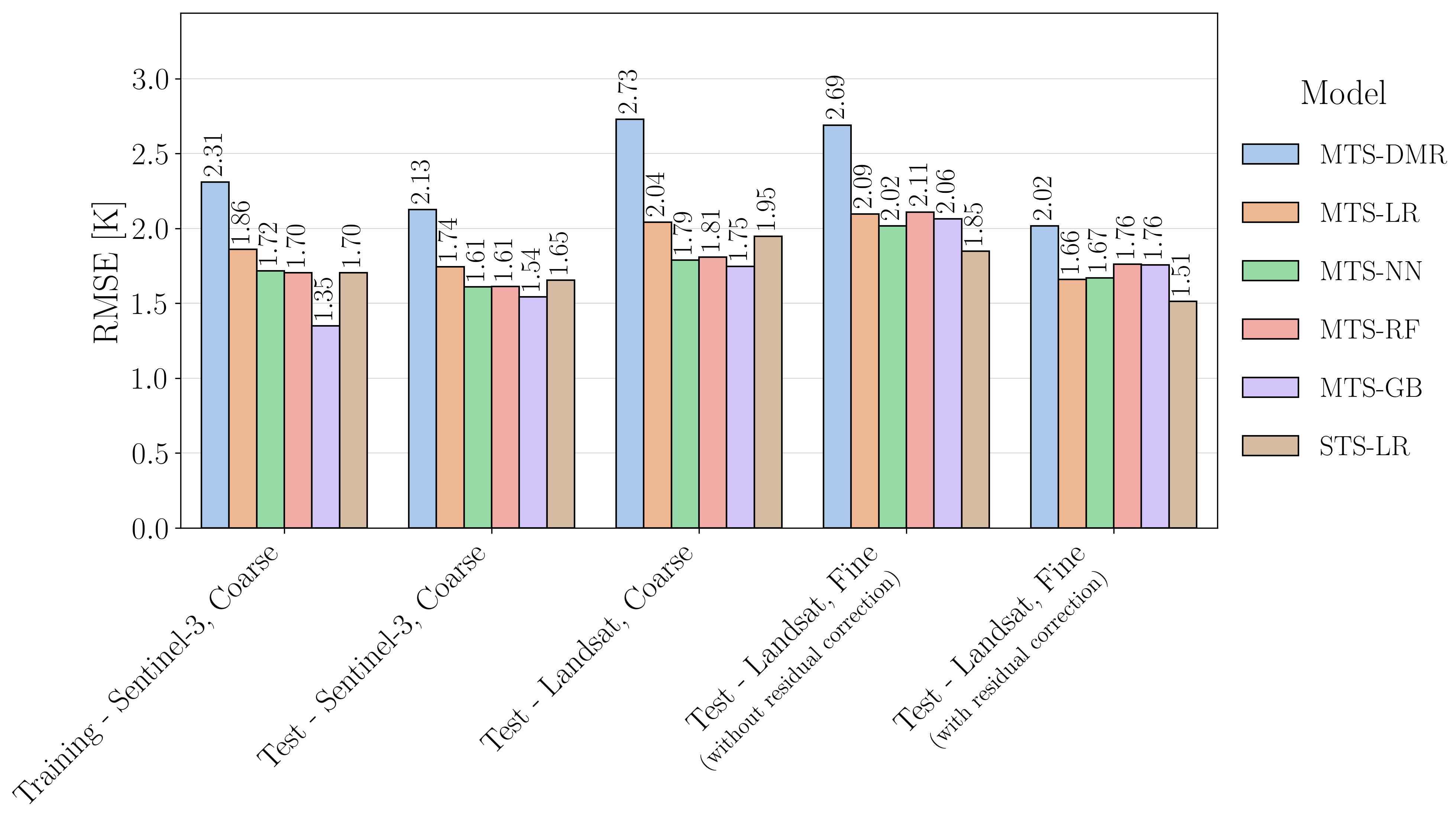
Figure 13 presents the RMSE values of all tuned MTS-ML downscaling models obtained in training and testing as well as the values of the MTS-LR model described in the previous section, an STSLR model using the same numerical predictors as this MTS-LR model, and the benchmarking MTS-DMR model. The figure shows that in the case of coarse prediction when considering Sentinel-3’s coarse LST as a true target, in contrast with the MTS-LR, all ML-based models performed better than STS-LR. GB was found to be the best coarse predictor, however, with significant overfitting—the figure shows a training RMSE value for GB ( 1.35   K ) that is significantly smaller than the respective coarse test one ( 1.54   K ). Conversely, the STS-LR model produced coarse training and test RMSEs of 1.70 and 1.65 K , respectively. NN and RF performed in an identical manner, producing a test RMSE of 1.61 K.
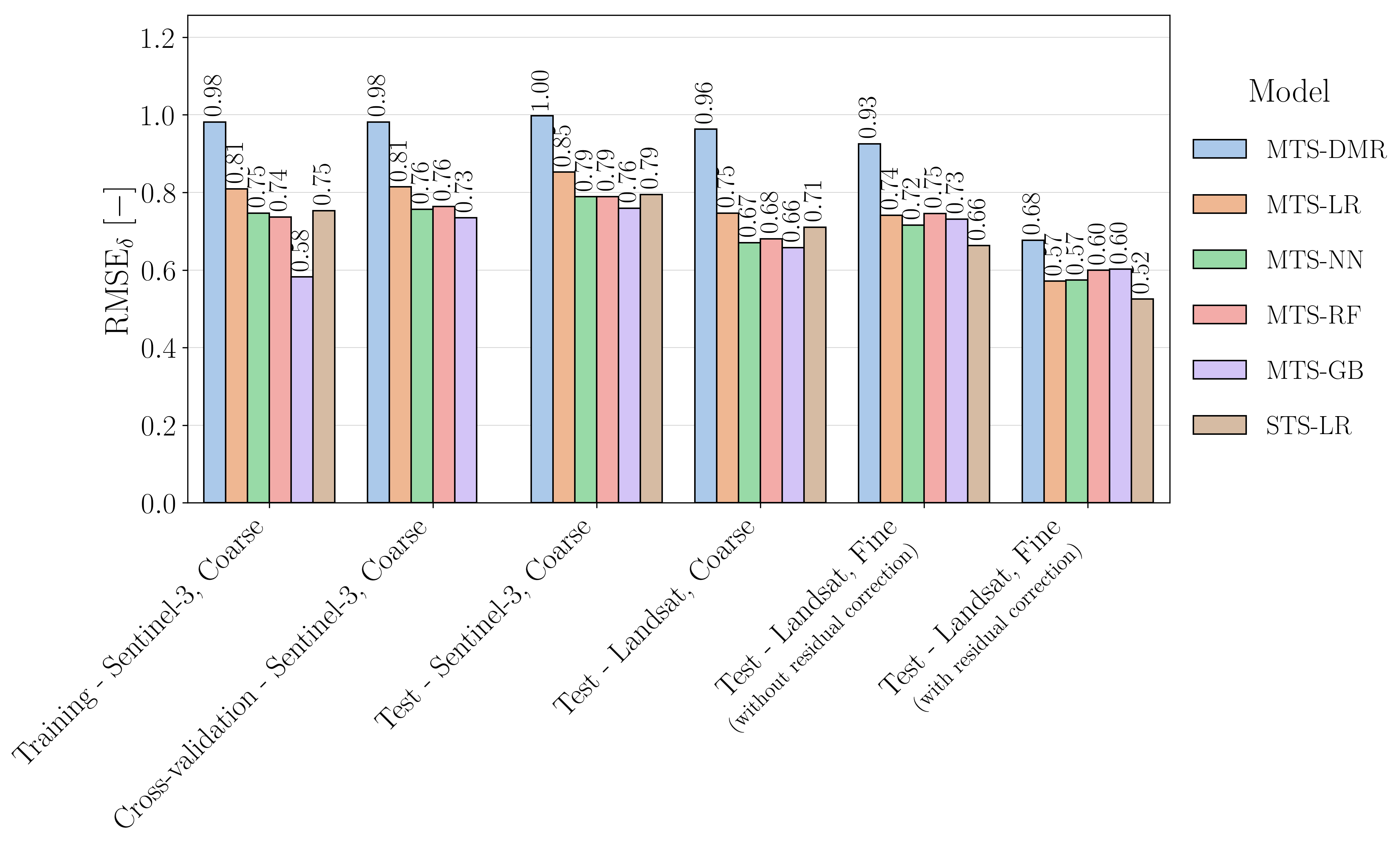
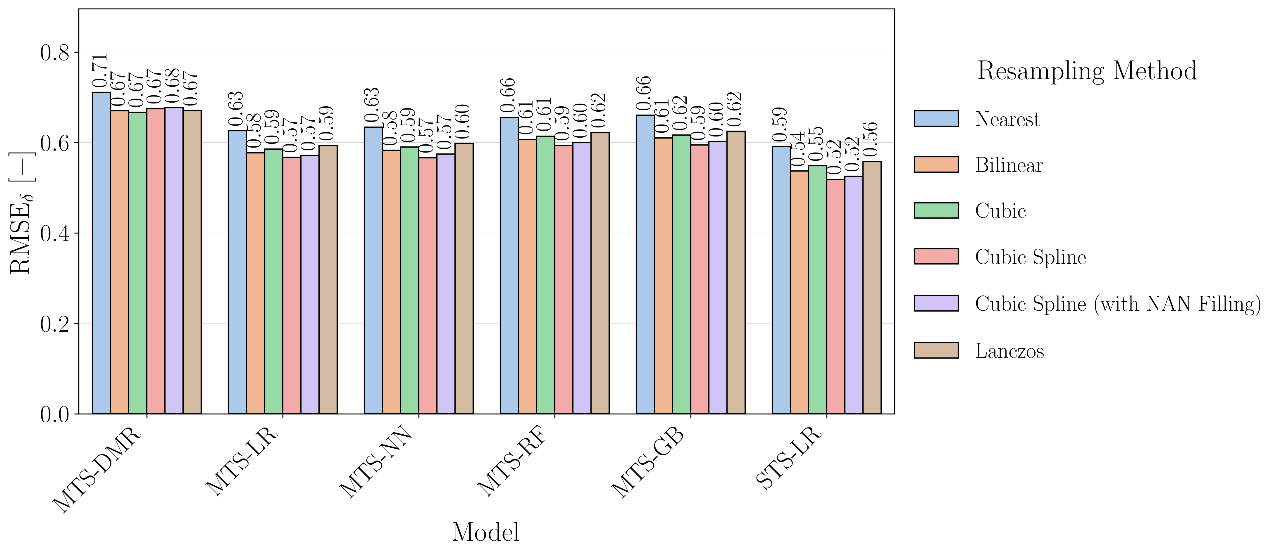
When considering coarsened Landsat’s LST as true target, even though all RMSE values increase, the relative differences between them remain approximately the same except for the case of the DMR model whose performance more abruptly worsens. The general increase in the RMSE values does reveal the occurrence of substantial differences between the native and validation data. Indeed, one finds the mean absolute difference between Sentinel-3 and Landsat’s coarse LST to attain almost 1 K (0.98 K). When comparing fine prediction not considering residual correction with coarse prediction having Landsat’s coarsened LST as the true target, one finds the RMSE values of all multi-timestamp models, especially the ML-based ones, to significantly increase, which may lead to the conclusion of the hypothesis of scale invariance not holding well for these latter architectures. Indeed, while the STS-LR value decreased, and the multi-timestamp counterpart one solely increased by 0.05 K (2%), the values of the ML models worsened significantly: by 0.23 K (13%) for the case of NN, 0.30 K (17%) for the case of RF and 0.31 K (18%) for the case of GB. The error of the tree-based models attained approximately the same value as MTS-LR’s which performed significantly worse in coarse prediction. Note, nonetheless, that an increase in RMSE from coarse to fine prediction could also be associated with a greater dispersion of the fine LST values. A fairer comparison would instead be based on RMSE δ values, that is, on the RMSE of the standardised predicted LST using the true LST statistics in the standardisation. Figure 14 presents such RMSE δ values. In this case, the STS-LR value decreases, the MTS-LR one barely changes, but the values of the ML models still significantly increase. From these results, one may conclude that a better fit of the ML models at the coarse scale herein implied a worse fit at the fine one and therefore also a disruption of scale invariance hypothesis. The tree-based models (RF and GB) revealed to be particularly affected by this disruption. This may be explained by the fact of these models, as in the case of all the others, having been trained with coarse data which do not contain the distribution tails of the fine data. And since tree-based models are equivalent to piecewise functions whose predicted values are constrained to the training domain, they tend to perform suboptimally when extrapolating.
One additionally finds from Figure 13 that residual correction in fine prediction makes all RMSE values significantly decrease. In this case, RF and GB unequivocally become the worst performers (with RMSE values of 1.76 K), NN now performs slightly worse than the MTS-LR model (with an RMSE value of 1.67 against 1.66 K) and the STS-LR model remains the best of them all (with an RMSE value of 1.51 K). One finds the MTS-LR model to consistently perform worse than the STS-LR model for all global coarse and fine prediction tests, even though the former has a higher complexity than the latter (it additionally contains season-specific intercepts and slopes with respect to the spatio-temporal predictors). This result further suggests that the multi-timestamp architecture may actually not provide an improvement of performance over that of its single-timestamp counterpart. This conclusion, however, cannot be directly extrapolated to the case of ML models, since no comparison against single-timestamp ML counterparts was done in this work.
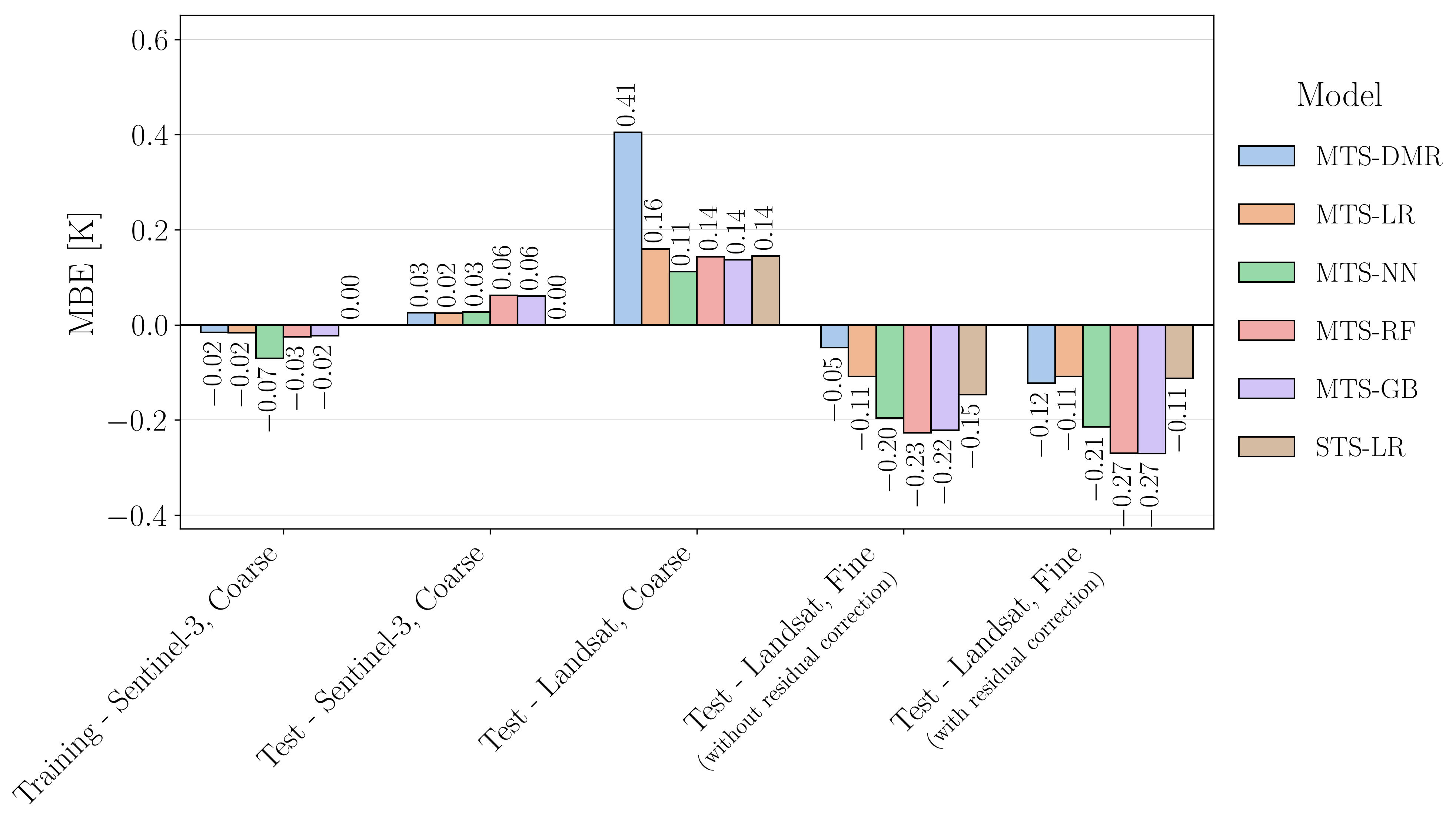
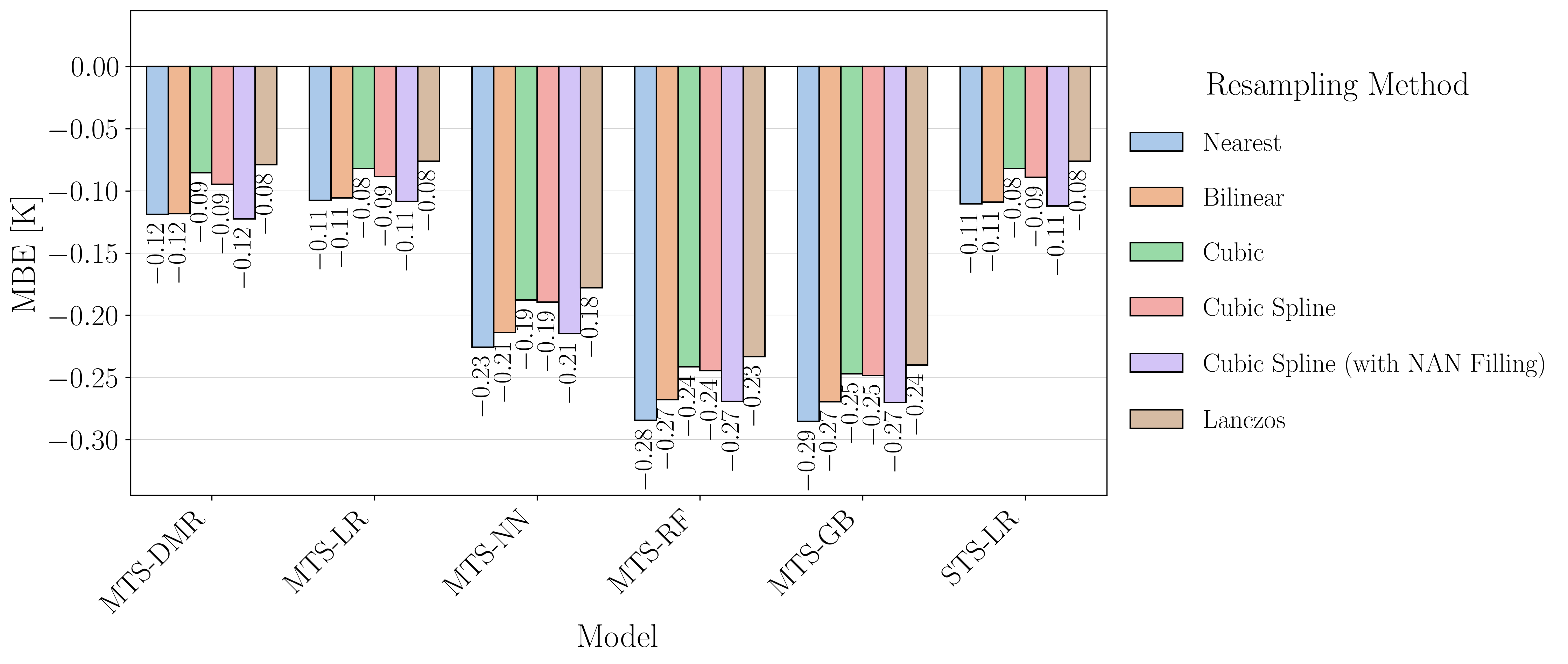
Breakage of scale invariance may also reveal itself through the values of the Mean Bias Error ( MBE ) of the tuned downscaling models. Figure 15 shows that the ML models, especially the tree-based ones, produce significantly negative MBE values in corrected fine inference, revealing tendency for underprediction. This clearly shows that the coarse relation learnt by the most complex downscaling models is actually different from the true fine one or that such coarse relation lacks support for the extreme values of the fine target, namely those at the higher limit. Indeed, and in the case of the tree-based models, since these cannot predict target values beyond the limits of the training domain, substantial underprediction by them could occur due to suboptimal performance at the high extremes of the fine data. The better MBE values obtained by the other models, which can indeed extrapolate beyond the training limits and actually performed worse than or as good as the tree-based models in coarse prediction, do provide further evidence supporting this hypothesis.
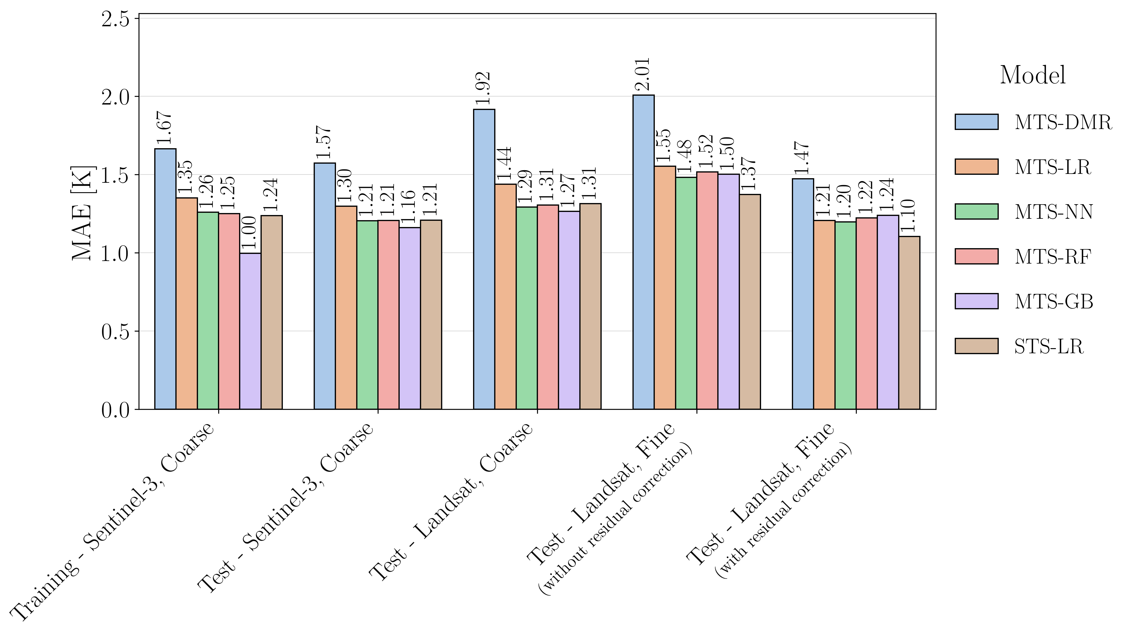
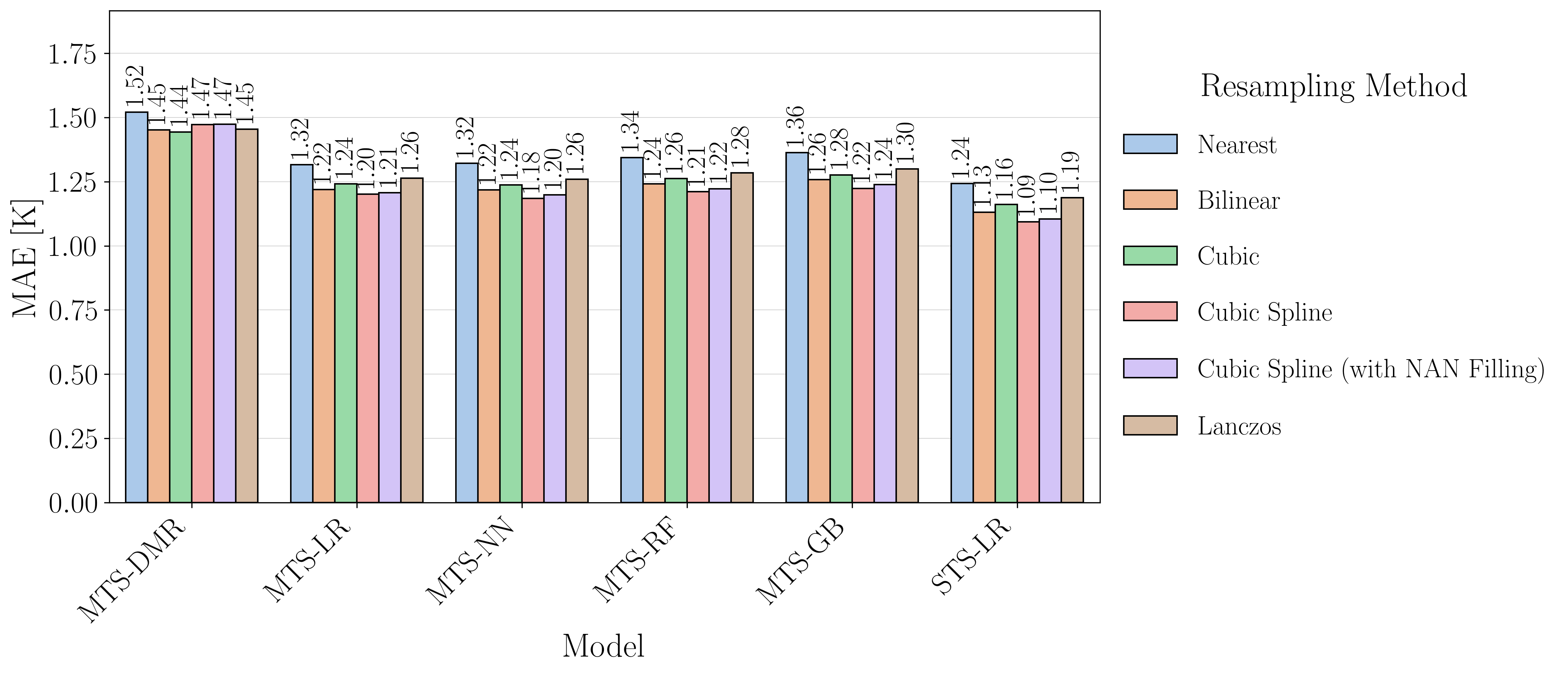
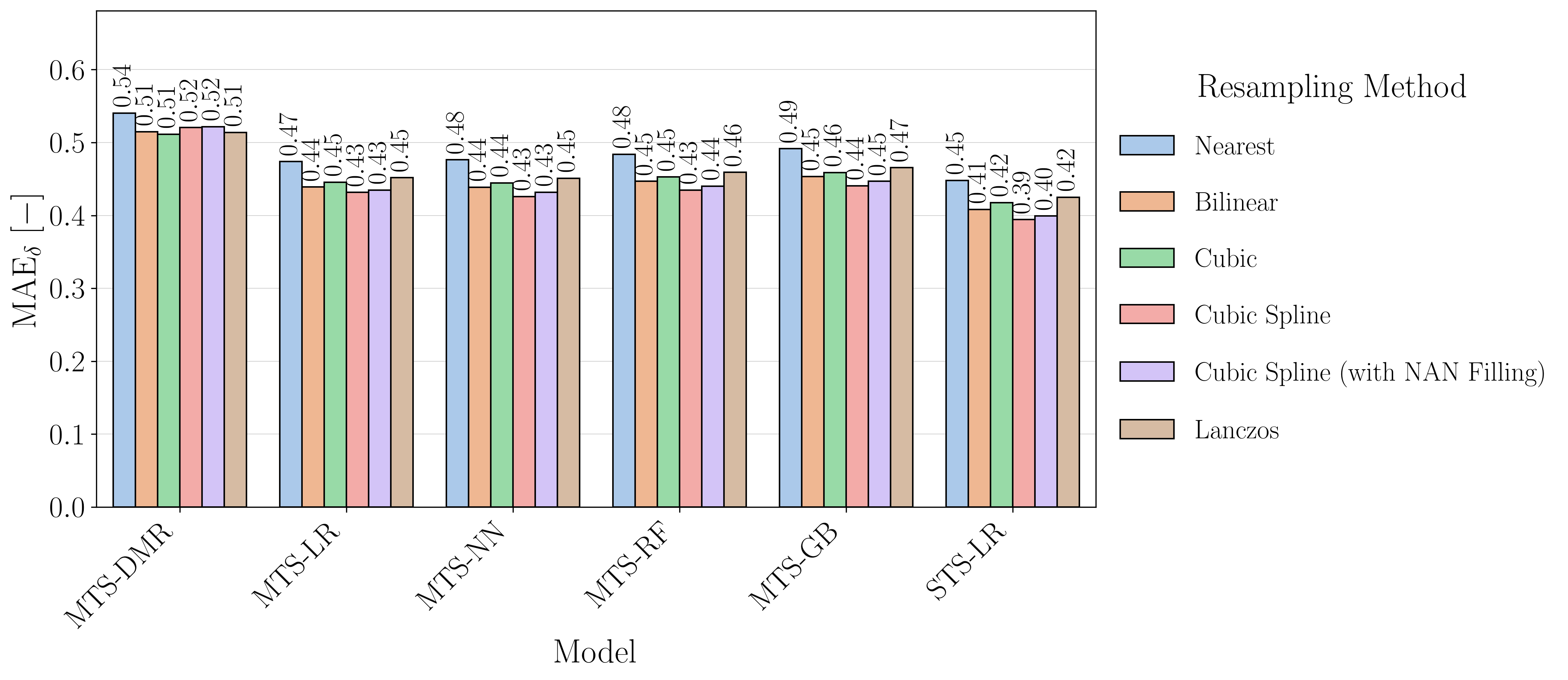
Figure 16 presents the respectively obtained MAE values. One finds the relative differences between models in this metric depart from those of the RMSE. For the case of coarse prediction, not all MAE values of the ML models are unequivocally smaller than STS-LR’s as happened with the RMSE values, but they are smaller or identical. However, for the case of uncorrected fine prediction, one finds the MAE values of all ML models to be smaller than MTS-LR’s when MTS-RF’s RMSEs were larger. And the relative MAE difference between models in corrected fine prediction is found to be not so significant as it is for RMSE, to the point of NN now appearing to perform slightly better than MTS-LR (when previously it did not). The differences in the relative distributions of MAE and RMSE values may be explained by the fact of the RMSE metric involving squaring of the individual errors, therefore weighing the values with larger magnitude more than the ones with smaller magnitude while MAE weighs them identically. One may then hypothesise from this that, in fine prediction, ML models produce more extreme individual errors than the LR ones while in coarse prediction the inverse tends to occur.

3.4. Distributions of the Downscaled Target

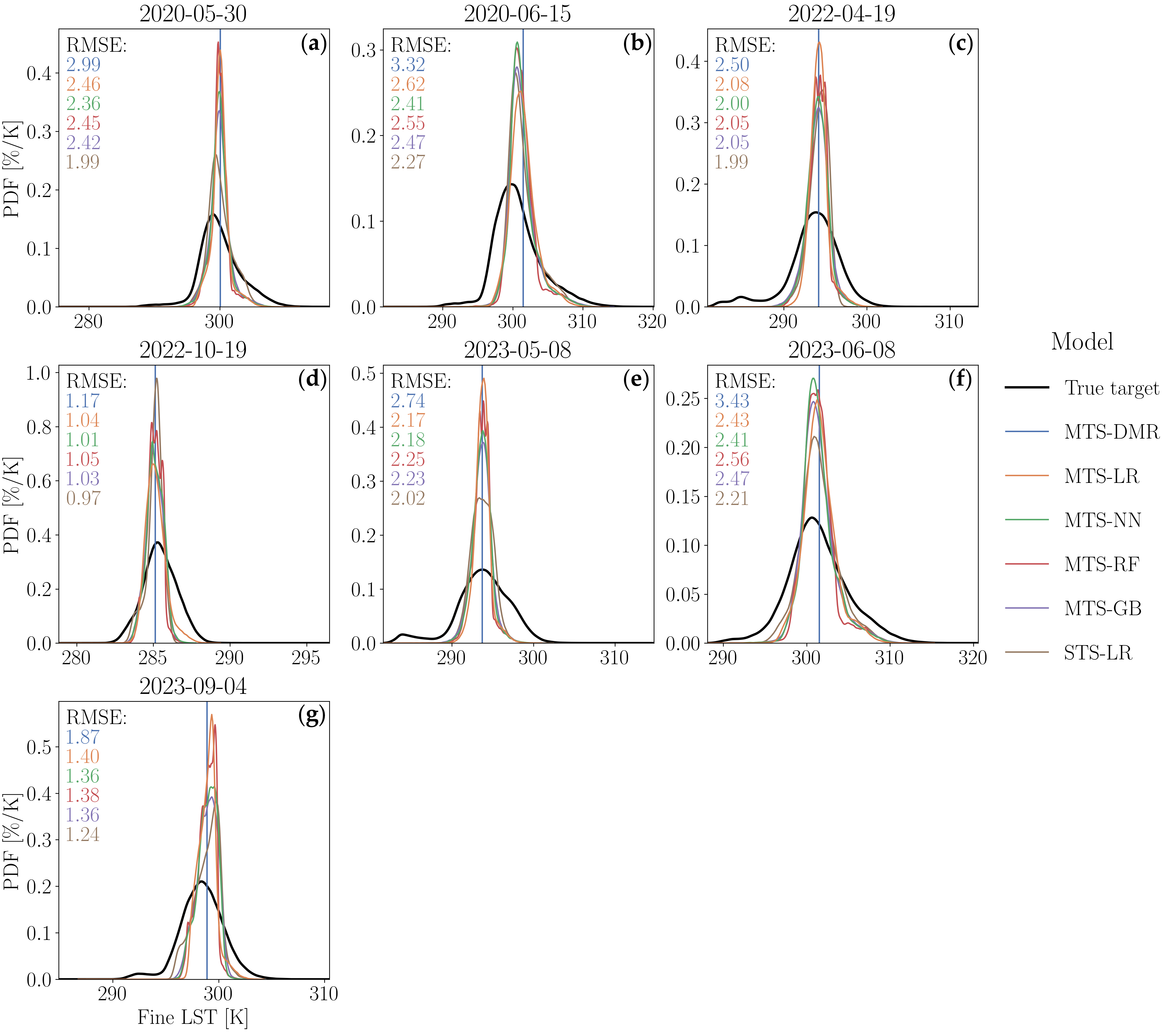
To further prove how scale invariance does not hold particularly well in the current problem, the Probability Density Functions (PDFs) of the actual and predicted fine LSTs without residual correction for all test timestamps are plotted in Figure 17. Overall, one finds the PDFs of the predicted values to be much thinner than the PDFs of the actual values for all models, which shows that these cannot predict the tails of the true distribution. Also note that, in the case of the DMR model, the PDF corresponds to a Dirac delta function centred on the mean of Sentinel-3’s coarse LST for each timestamp.
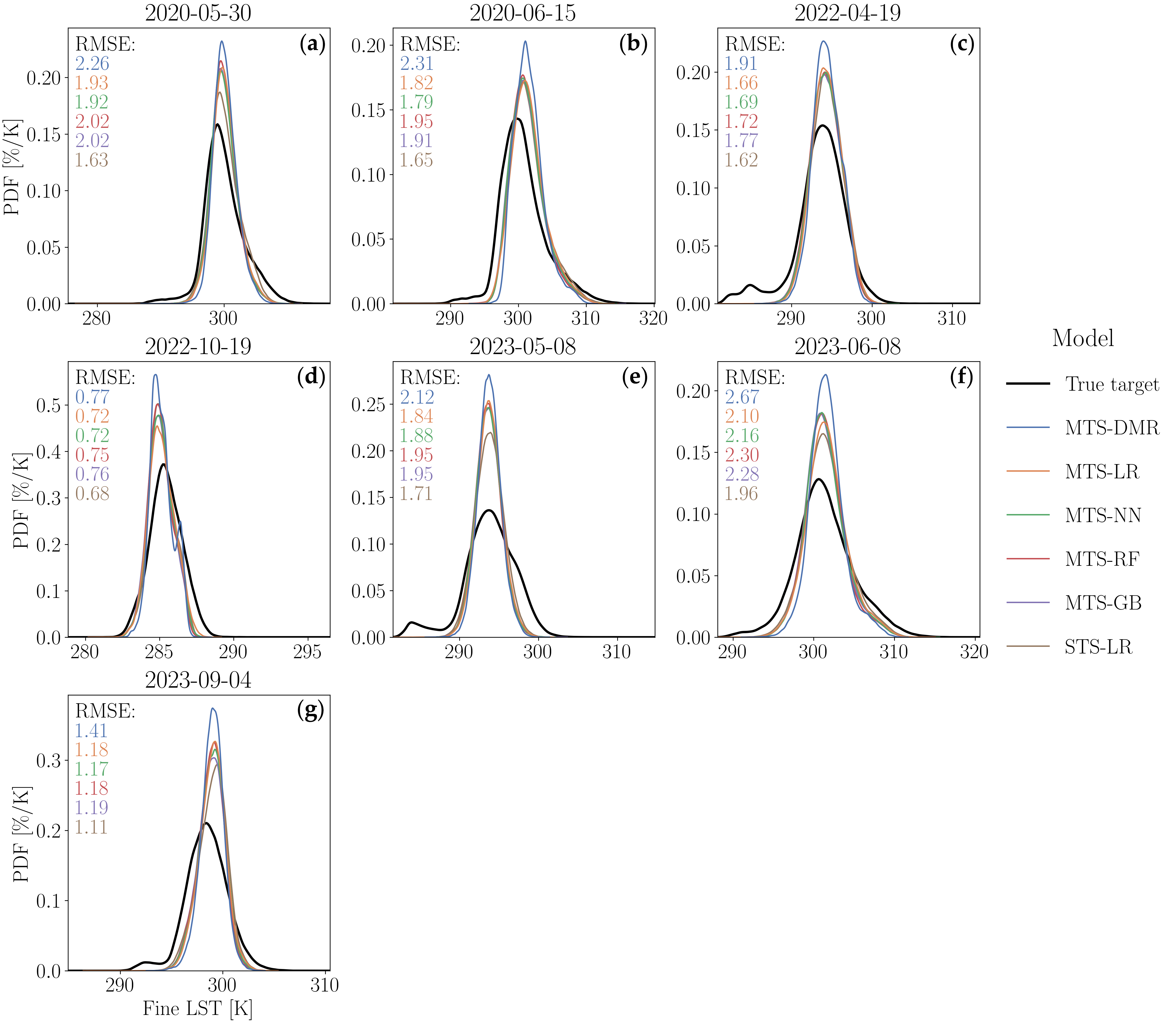
Fortunately, residual correction quite effectively compensates for the error involved in the scale invariance assumption, as it makes the predicted and actual PDFs reasonably agree with each other—as shown by Figure 18. The DMR PDF remains distinctively thinner than the ones for any other model, revealing that pure fine interpolation more difficultly estimates the extreme values. The figure also presents the RMSE values of the fine predictions (with residual correction) obtained by each model for each test timestamp, showing that the single-timestamp LR model not only produces the smallest global RMSE value but also the smallest particular one for every single timestamp.

3.5. Distributions of the Downscaling Error

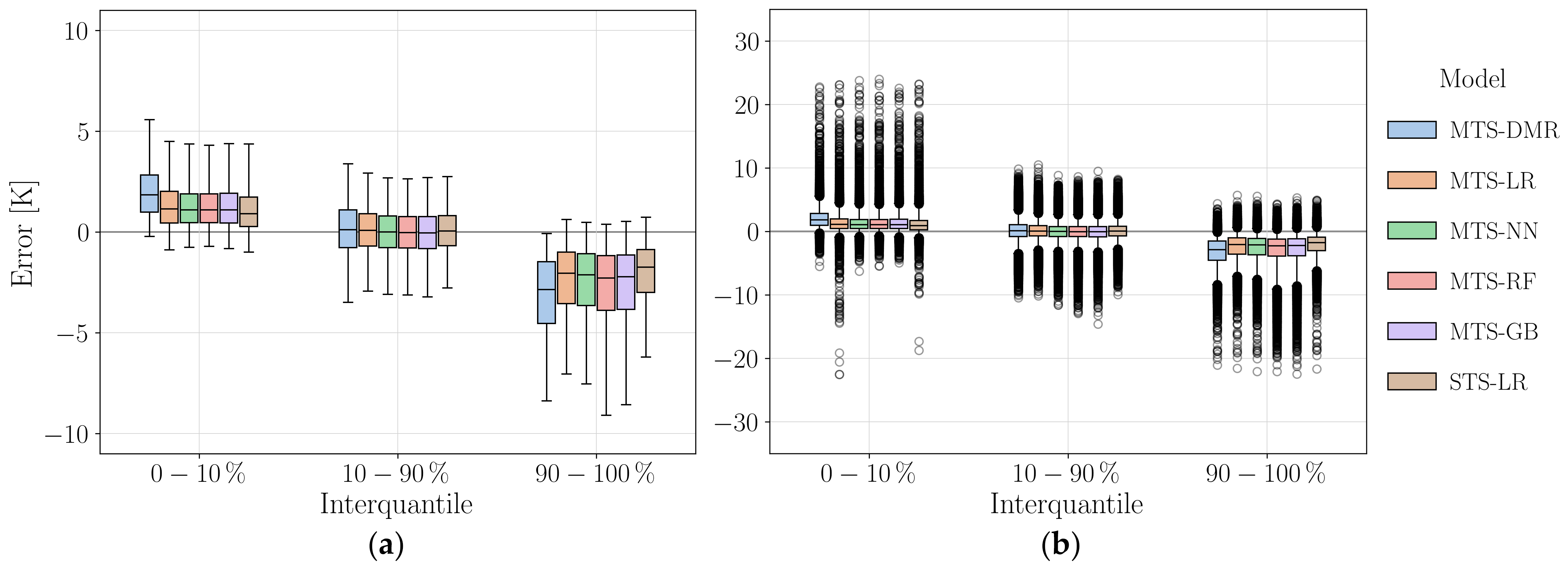
To better ascertain how the models perform at the distribution tails of the fine LST , Figure 19 presents boxplots of the test fine prediction error (with residual correction) obtained by each model for different interpercentiles of the true fine LST : between 0 -th and 10 th, 10 -th and 90 th, and 90 -th and 100 th percentiles. Note that, since the extreme values of each timestamp and not of all of them combined are wanted, the computed percentiles are timestamp-specific. To better visualise the distributions, the outliers were removed in the subfigure on the left-hand side (a) but not in the subfigure on the right-hand side (b). In both subfigures, the boxplot whiskers are constrained to the 2 nd and 98 th percentiles of the error distributions. The subfigure on the left-hand side (a) shows that the STS-LR model is the one that best performs at both extreme interquantiles. The tree-based models are found to be worse than all others at the higher extreme interpercentile. Although the multi-timestamp LR and NN models show comparable performance at this higher extreme, the NN model and particularly the tree-based ones exhibit a tendency towards a slight underprediction within the intermediate interquantile range, therefore contributing to the higher negative mean bias error that had been previously observed. These results further evidence the already mentioned breakage of scale invariance that appears to be significant for the case of the ML models. The subfigure on the right-hand side (b), reveals the presence of quite large outliers in the error distributions, with some attaining almost 25   K in magnitude, which merit further investigation.
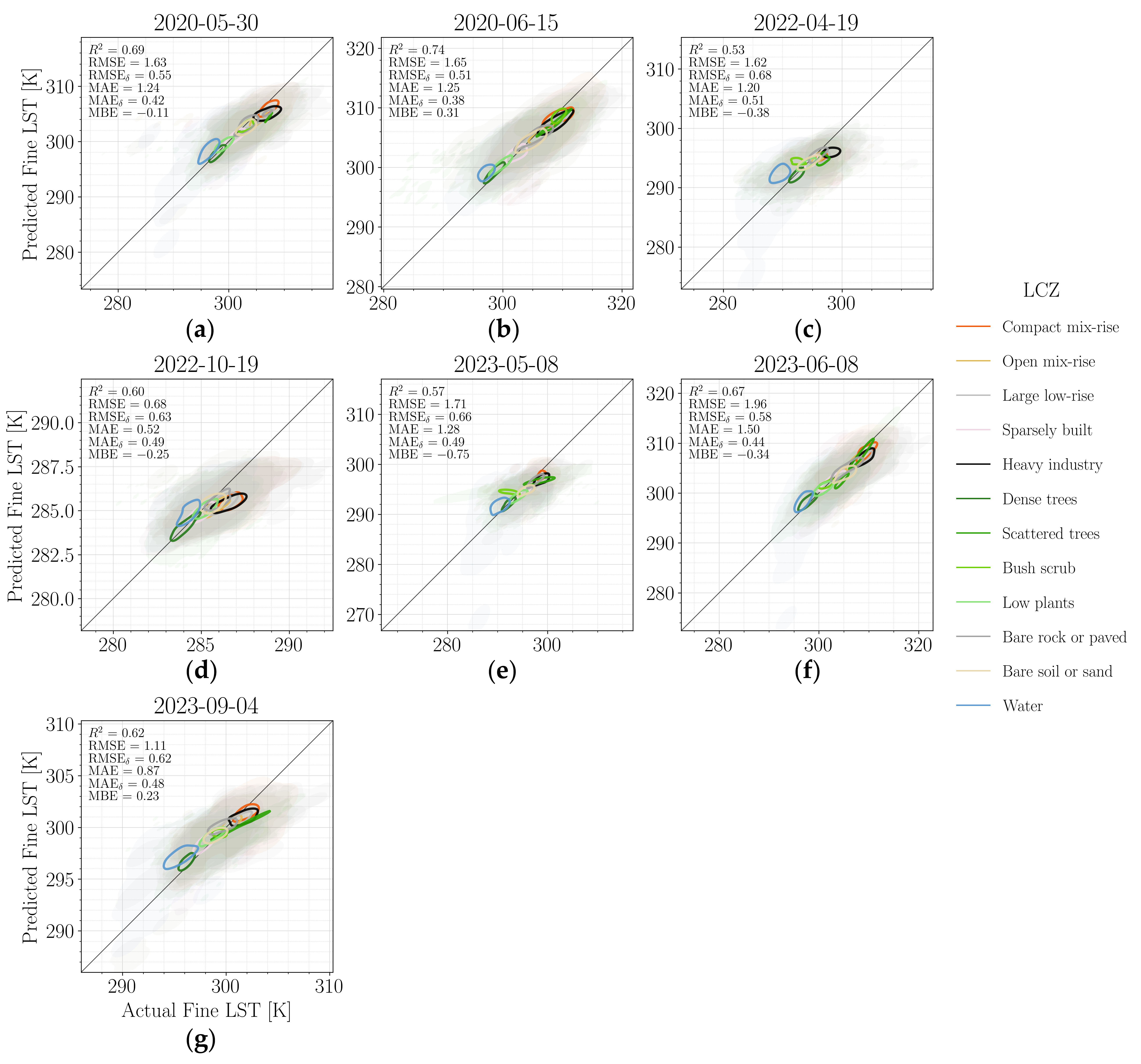
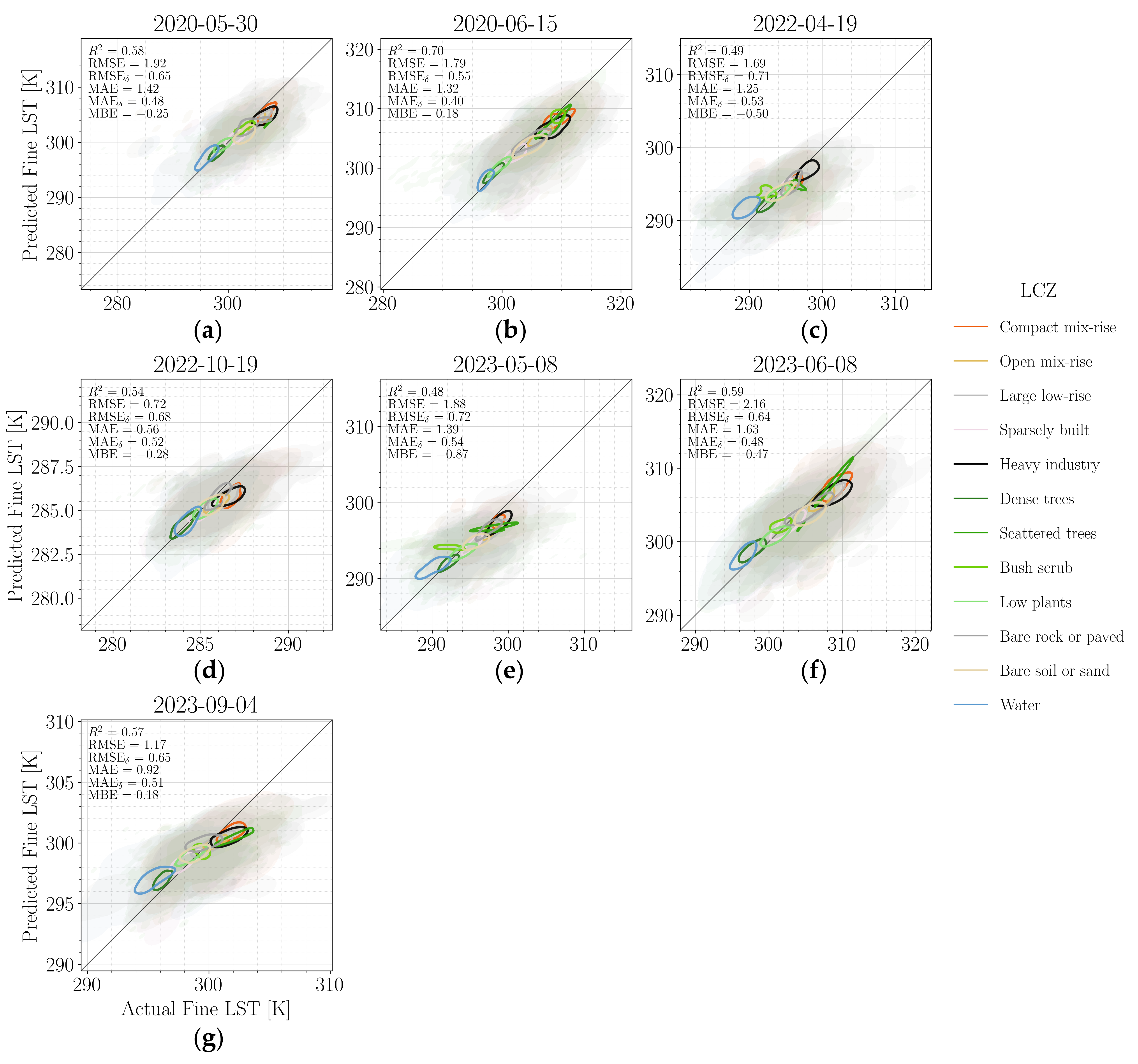
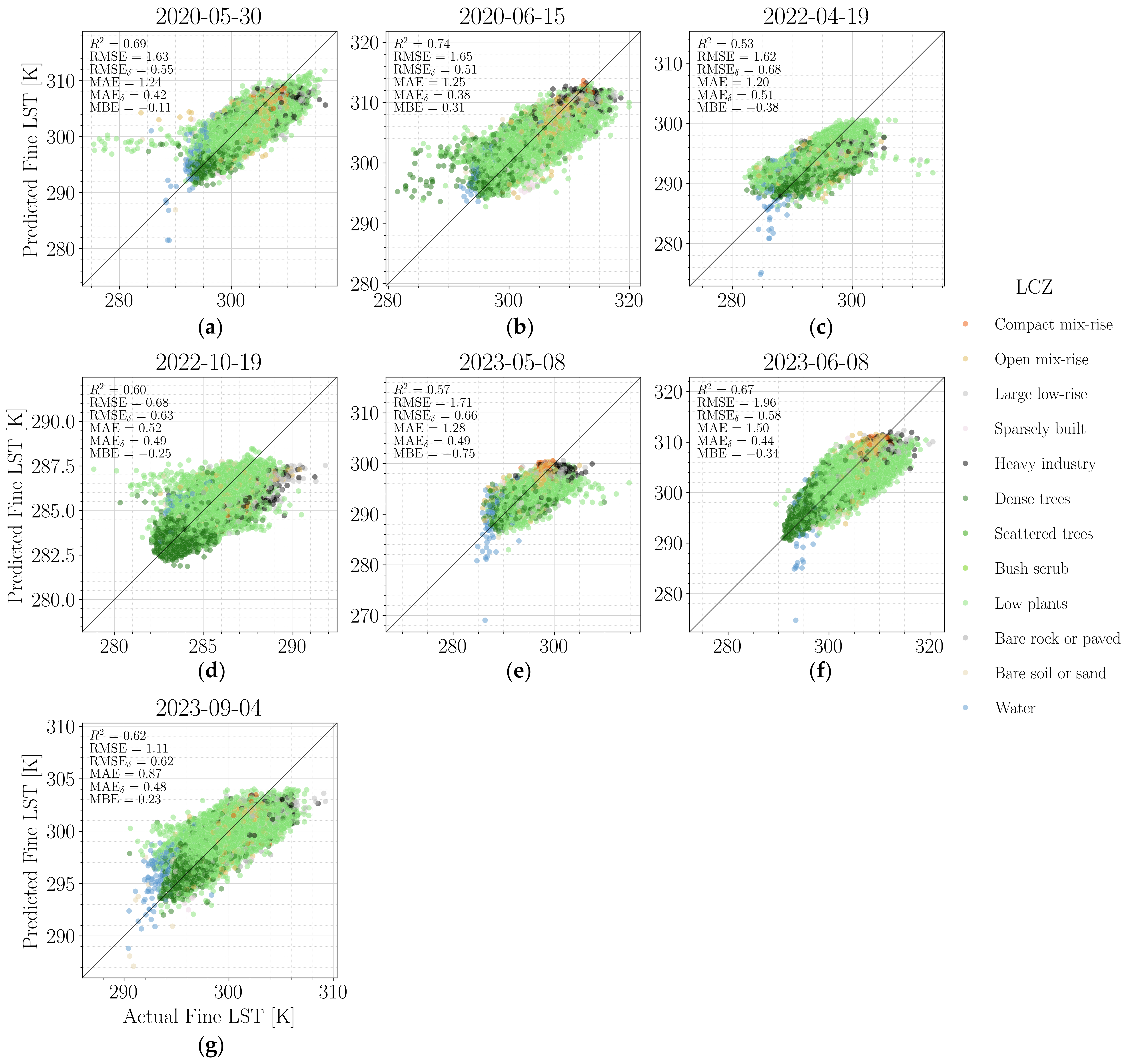
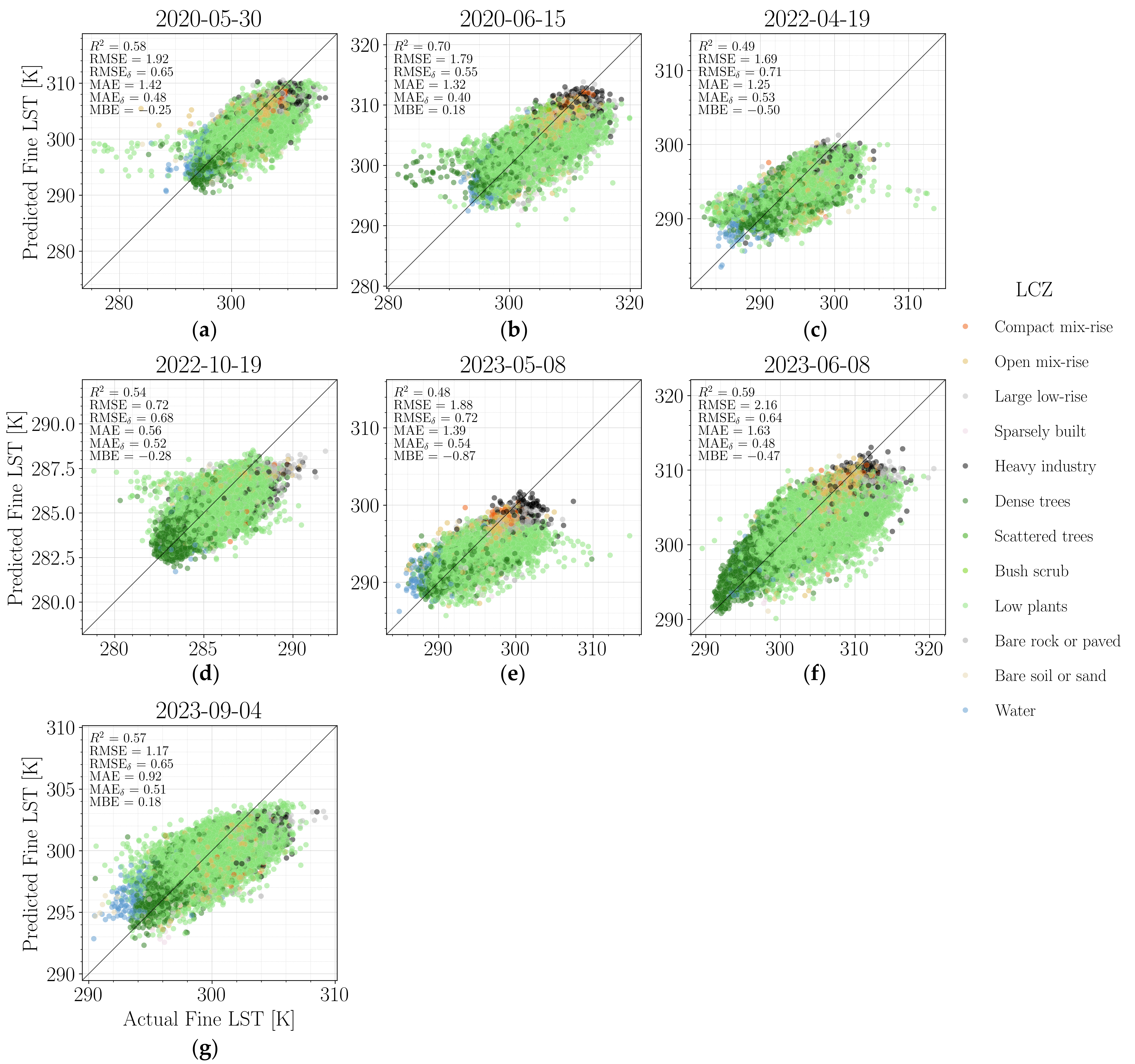
One may visualise the errors within more detail through a predicted-vs-actual plot for the fine LST hued by Local Climate Zone ( LCZ ). Figure 20 and Figure 21 present such plots for the case of the STS-LR and MTS-NN models, respectively. These figures reveal the water bodies and dense trees to be associated with the smallest LST values; sparsely built and bare soil or sand with the medium values; and heavy industry, compact mix-rise and scattered trees with the high values. Moreover, the values of the low plants mostly swing between low and medium temperatures; the ones of bare rock or paved zones, large low-rise and open mix-rise may be between medium and high; and those of bush scrub typically vary within the whole range. Note that low plants comprise most of the data (72%, as shown by Figure 7) and, because of this, the obtained metrics are strongly associated with models’ performance at pixels where they occur. The LST values of the low plants, in fact, appear to be reasonably well estimated, without a tendency for being under- or overpredicted by both models. The temperatures of the zones at the low and high extremes, however, do tend to be over- and underpredicted, respectively, showing how the models give greater importance to the intermediate interval which is much more common and also associated with the quite predominant low plant zones. The equivalent scatter plots of Figure A2 and Figure A3 in Appendix A.3 further show that the outliers at the highest LST values are associated with underprediction in low plants, large low-rise and heavy industry zones while the ones at the lowest LST values are associated with overprediction for low plants, dense trees and open mix-rise, and, in the case of the STS-LR model, also underprediction for bare soil or sand and quite prominently for water bodies. This latter strong underprediction was, in fact, solely observed for the case of the LR models. This reveals how the relationship between target and the predictors is in fact non-linear, that is, the way the former varies with respect to one of the latter does concomitantly depend on the others. In this case, it appears to significantly depend on whether the zone corresponds to water or not. Such a property, in turn, may be described by some set of predictors, which when used in a non-linear model can properly represent the target (in contrast with the case of a linear model). This further shows how in some cases the non-linear models may better “capture” particularities of the data than the linear ones.
One finds the distribution of points in the predicted-vs-actual plots to be, overall, wider—therefore, being associated with a larger error—for the multi-timestamp NN model than for the single-timestamp LR one.
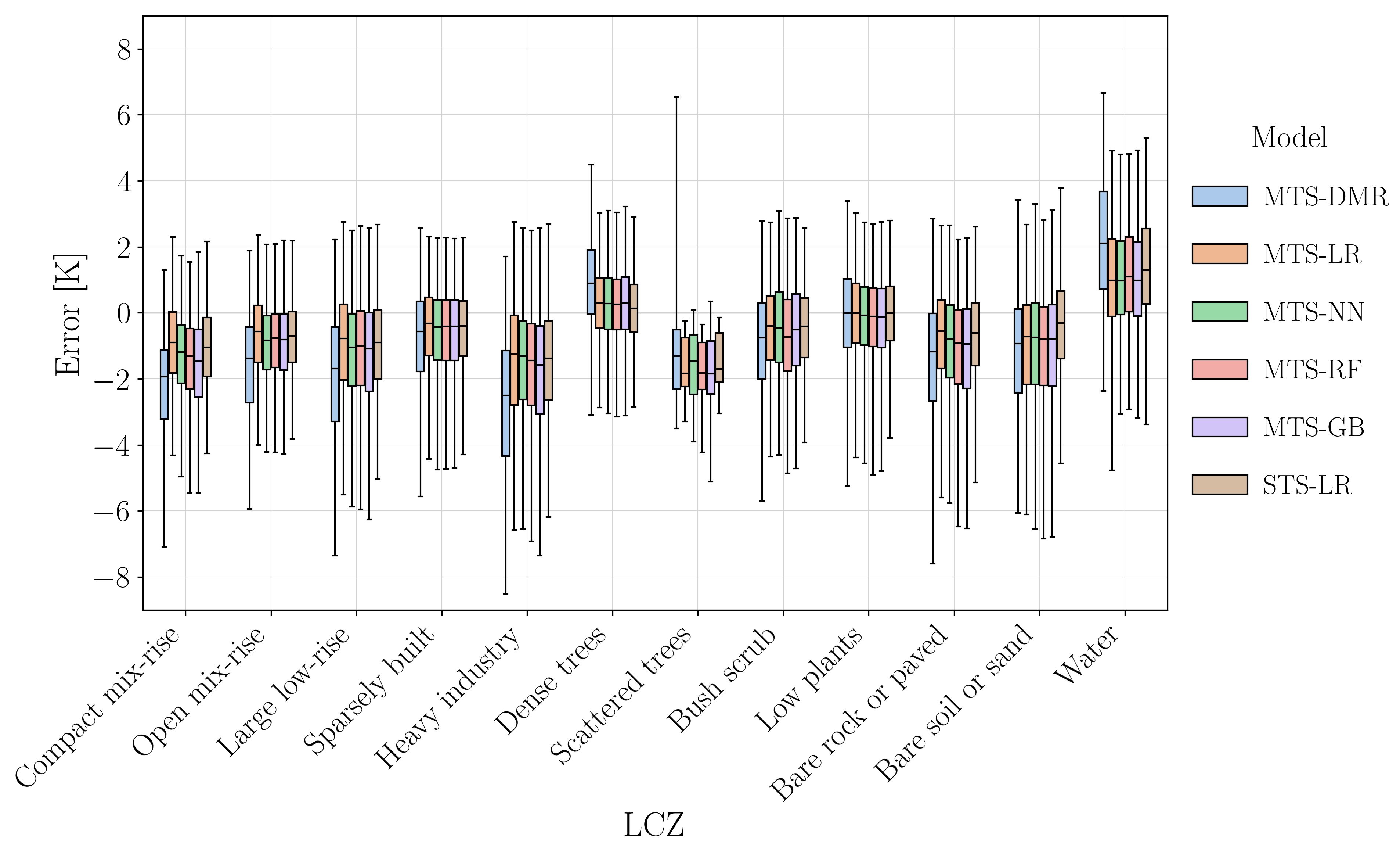
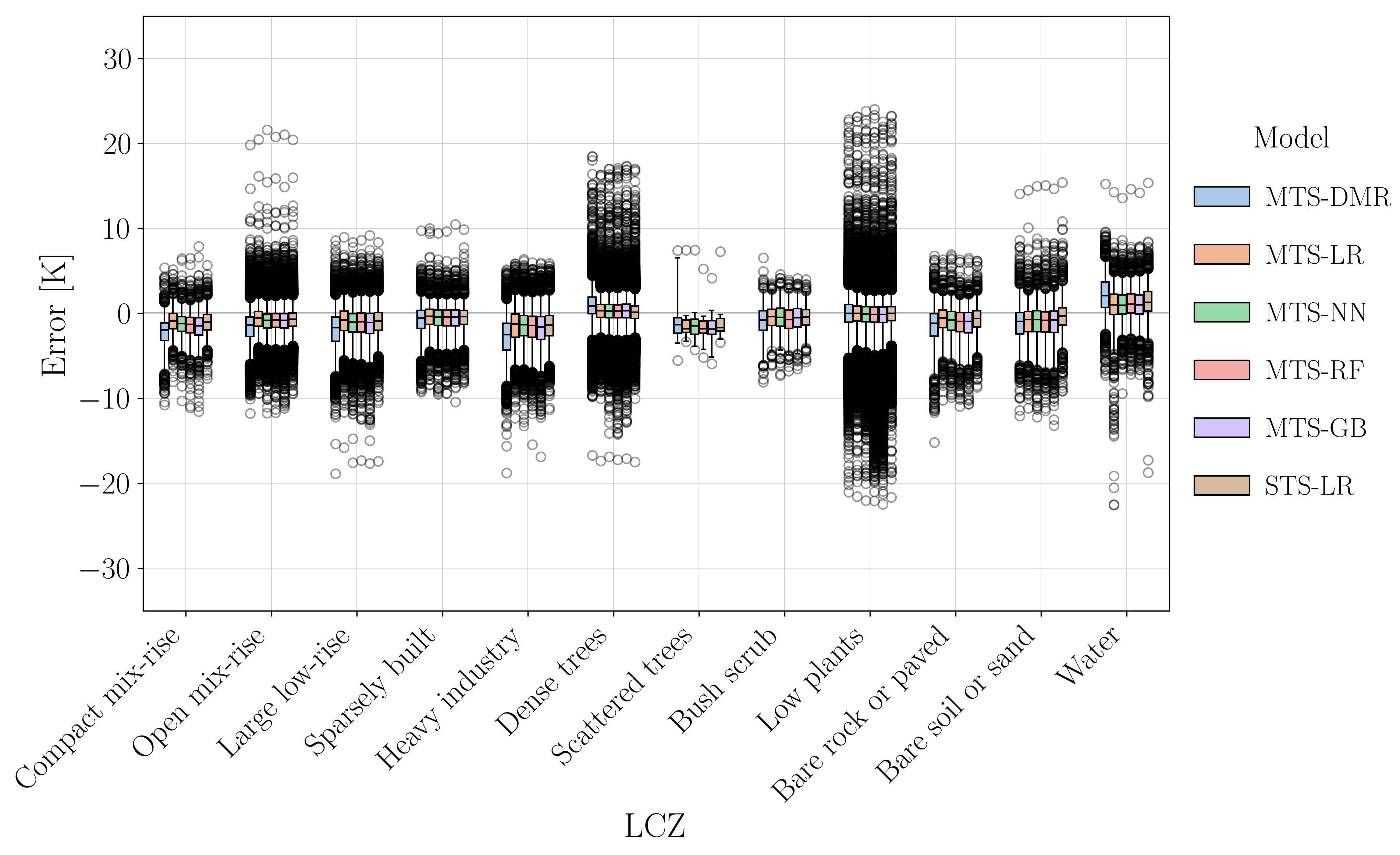
Figure 22 and Figure 23 present boxplot distributions of the test’s fine prediction error (with residual correction) obtained by the downscaling models for each LCZ class, without and with outliers, respectively. The interpretation of these figures could in fact provide a more accurate assertion on whether under- or overprediction of the target occurs for each zone type. The figures show that most classes have a tendency for being underpredicted rather than overpredicted. In fact, solely the values of dense trees and especially water bodies (the zones typically associated with smallest LST values) tend to be overpredicted. The values of low plants (the most dominant zone type) are prone to neither under- nor overprediction. The values of all the others, which are mostly associated with built-up or open areas, with less vegetation, tend to be underpredicted (as these typically attain higher temperatures). Figure 23 shows that the largest errors occur for open mix-rise, large low-rise, heavy industry, dense trees, low plants, bare soil or sand, and, in the case of linear models—as previously mentioned—also water bodies.

3.6. Outlying Downscaling Errors

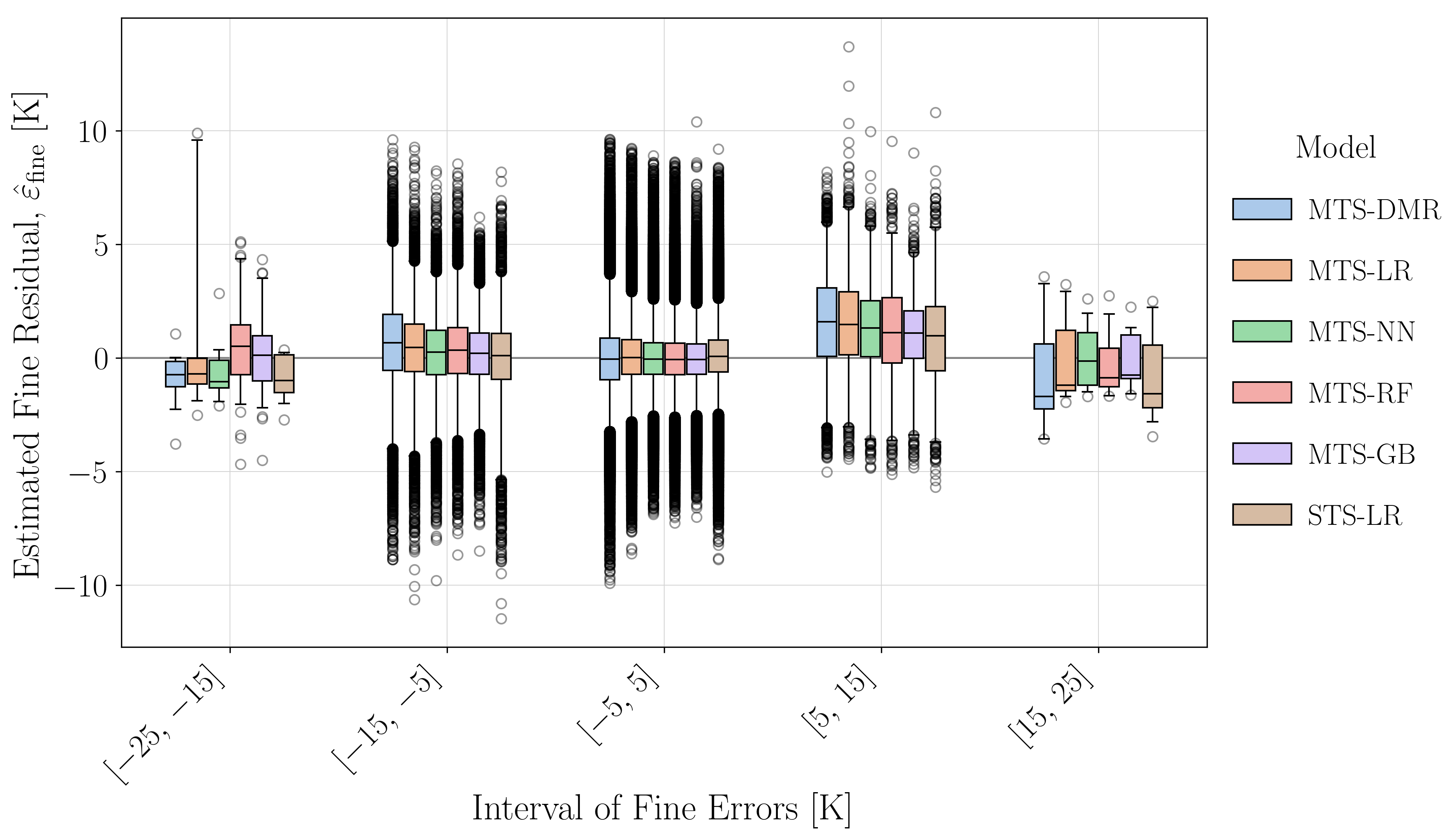
Figure 23 reveals that, although extremely rare, errors of very large magnitude may occur, of nearly 25 K . Indeed, the outlying error values obtained by the different models are even comparable to the ones obtained by DMR. This suggests that such errors probably originated from highly incorrect fine estimations which simultaneously contrast with reasonable coarse ones, not allowing the former to be corrected by the residuals of the latter. While such large fine errors may result from outlying fine predictor values (or from punctual disruption of the established predictor–target relationship), the simultaneous small coarse errors should result from moderate coarse predictor values—as these are obtained from a weighted average (therefore, involving smoothness) of the fine ones. To better assess the phenomenon, Figure 24 presents boxplot distributions of the estimated fine residuals (that is, the finely interpolated coarse residuals), | ε ^ fine | , for different ranges of the fine prediction errors obtained when considering residual correction: between 5 and 5 , 5 and 15 , 15 and 25 K and their symmetrics. The figure reveals that all quartiles (25-th and 75-th percentiles and median) of the residuals are consistently small (within the interval 5 , 5 ). One may then say that most of the obtained residuals are, overall, reasonably small throughout the whole range of errors, which further shows that the main cause of the extremely large fine prediction errors is an incorrect estimation of the fine target whose finely interpolated coarse prediction residual cannot compensate. This result suggests that that residual correction is highly ineffective for cases of extreme fine estimation error.
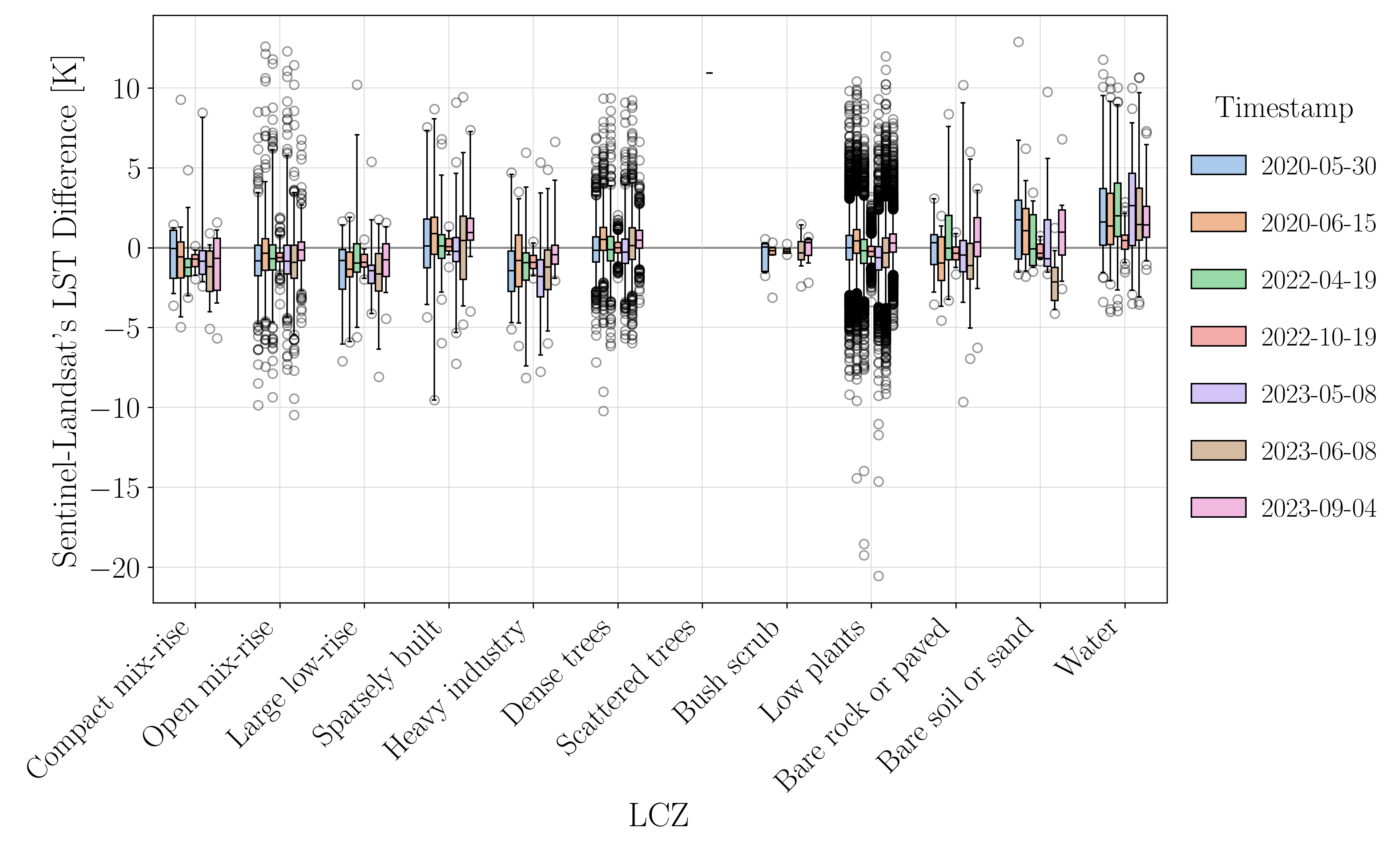
It is also possible that the extreme fine prediction errors derive from punctual high discrepancies between Sentinel-3 and Landsat data, with the latter being regarded as the supplier of ground-truth fine LST values. To assess this, boxplot distributions of the differences between Sentinel-3 and Landsat’s coarse LST values were obtained for the different timestamps and LCZ classes—as shown in Figure 25. The figure reveals that all quartiles of the differences are not too significant, being encompassed by the interval 5 , 5 K . This means that most of the data acquired by Sentinel-3 and Landsat should not differ too much from each other. However, the distributions do also show a considerable number of outliers that even surpass the 10 and 10 K limits, especially for open mix-rise, low plants and water—these were also some of the zone types for which strong outliers of the fine prediction error had been found. Moreover, note that coarsening involves smoothing, and, therefore, one could expect even larger differences in the fine grid. Such discrepancies seem to transcend all timestamps except 19 October 2022 for which they were found to be consistently small (being encompassed by the interval 5 , 5 K ). This exception may be explained by the fact of timestamp 19 October 2022 being associated with LST values with mean and standard deviation which are significantly smaller than those of any other—the Landsat LST data resampled onto Sentinel-3’s fine grid for this timestamp has indeed a mean and standard deviation of 285 and 1.1 K, respectively, while for all the others means between 293 and 301 K and standard deviations between 2.1 and 3.7 K were obtained. The smaller the values and their variability in the fine actual data, the smaller the differences with respect to the respective coarse data and the closer the downscaling results would get to the true values.
It is important to note that the current analysis and inferred conclusions assume weighted averaging to properly simulate coarse data from Landsat’s fine data. However, not only may differences between acquisitions platforms (in radiometric processing, geo-referencing and acquisition time) contribute to discrepancies in the respective original products but the errors from coarsening simulation may also make the products resampled onto a common coarser grid differ further.

3.7. Distributions of the Test Scores

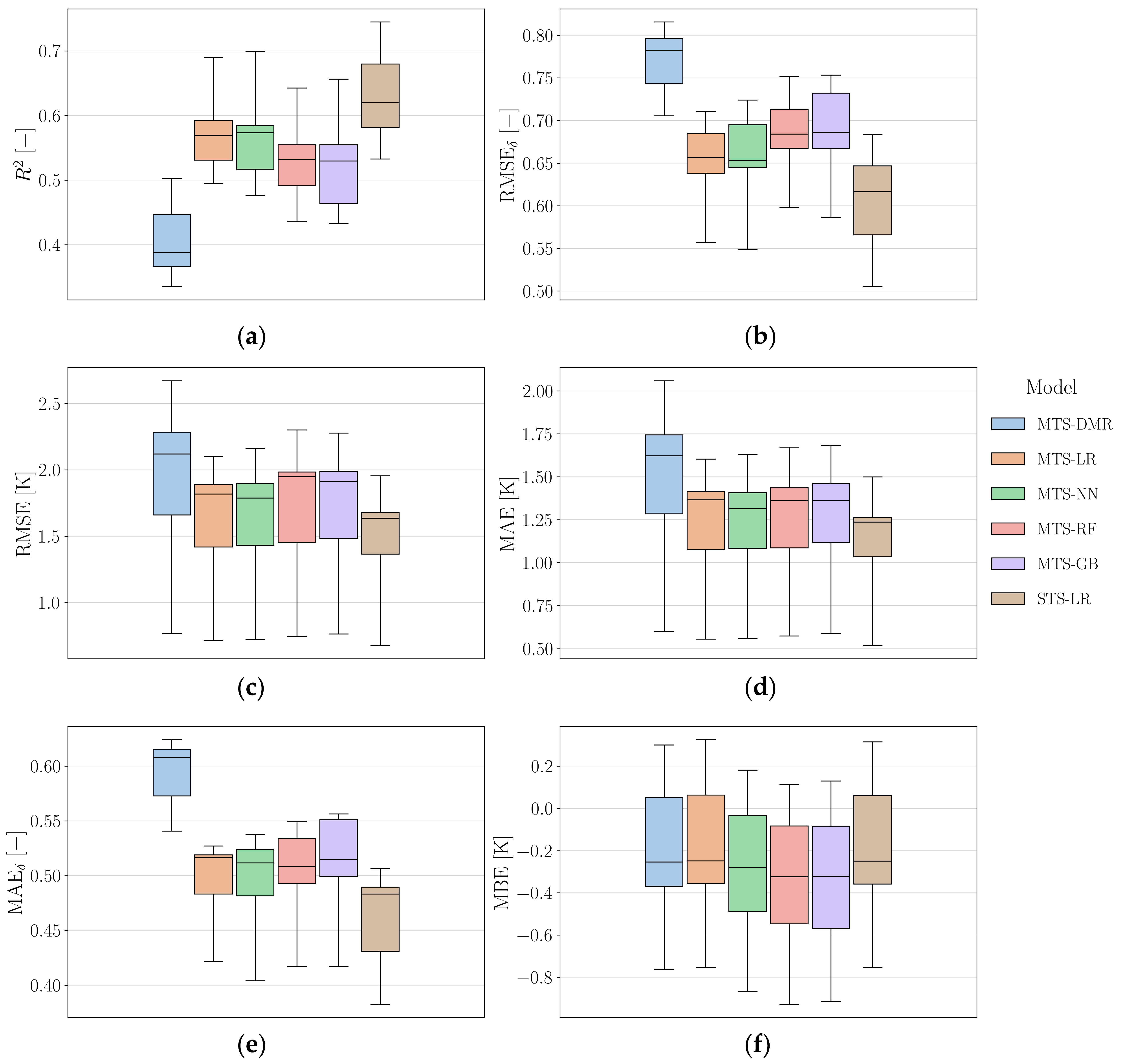
Figure 26 presents boxplot distributions of the fine metrics obtained by the models for the test timestamps when considering residual correction. Regarding R 2 , one finds single-timestamp LR to attain the highest upper limit ( 0.74 ), with the multi-timestamp NN and LR models coming second ( 0.70 ) and third ( 0.69 ), respectively. The tree-based models produced the smallest upper R 2 limits: 0.66 in the case of MTS-GB and 0.64 in the case of MTS-RF. Nonetheless, all models produced significantly larger R 2 values than DMR (which is equivalent to pure interpolation). Indeed, the smallest upper limit (MTS-RF’s 0.64) was larger than DMR’s (0.50) by 0.14) and the smallest lower limit (MTS-GB’s 0.43) was larger than DMR’s (0.33) by 0.10.
As previously stated, one should note that the test coarse Sentinel-3 and Landsat LSTs were correlated with a score of R 2   0.62 , and, therefore, that not much higher values could be expected for the fine test score of the downscaling models. However, even though the R 2 quartiles obtained with the different models were significantly smaller than this reference value, the distributions do encompass it, evidencing reasonability in downscaling performance.
The lowest R 2 values that were obtained by the all models except STS-LR are associated with timestamp 8 May 2023 followed by 19 April 2022. In the case of STS-LR, the lowest values are instead associated with this latter timestamp followed by the former. As shown by Figure A4, Figure A5, Figure A6, Figure A7, Figure A8, Figure A9 and Figure A10 of Appendix A.3 only these timestamps contain validation data for Copenhagen which Figure 6 reveals to be significantly more urbanised and heterogeneous than the remainder of the Danish FUAs. Similarly to many other works in the literature, the present results suggest that the largest downscaling errors are indeed obtained for such highly urbanised areas.
Regarding the MBE metric, one may say that all upper limits are positive and all lower ones are negative, showing that both under- and overprediction do occur. However, most values are below the neutral line, revealing underprediction to be more predominant, as previously concluded. The single and multi-timestamp LR models are the ones with the greatest upper limit ( 0.33 and 0.32 K , respectively), being similar to DMR’s ( 0.31 K ). And their lower limit ( 0.75 K ) is the one closest to 0 , also being similar to DMR’s ( 0.76   K ). The linear models are herein again found to be the ones with the smallest tendency for underprediction. Conversely, the RF and GB models are found to be the ones with the highest tendency, producing the most negative MBE values.

3.8. Maps of the Downscaled Target

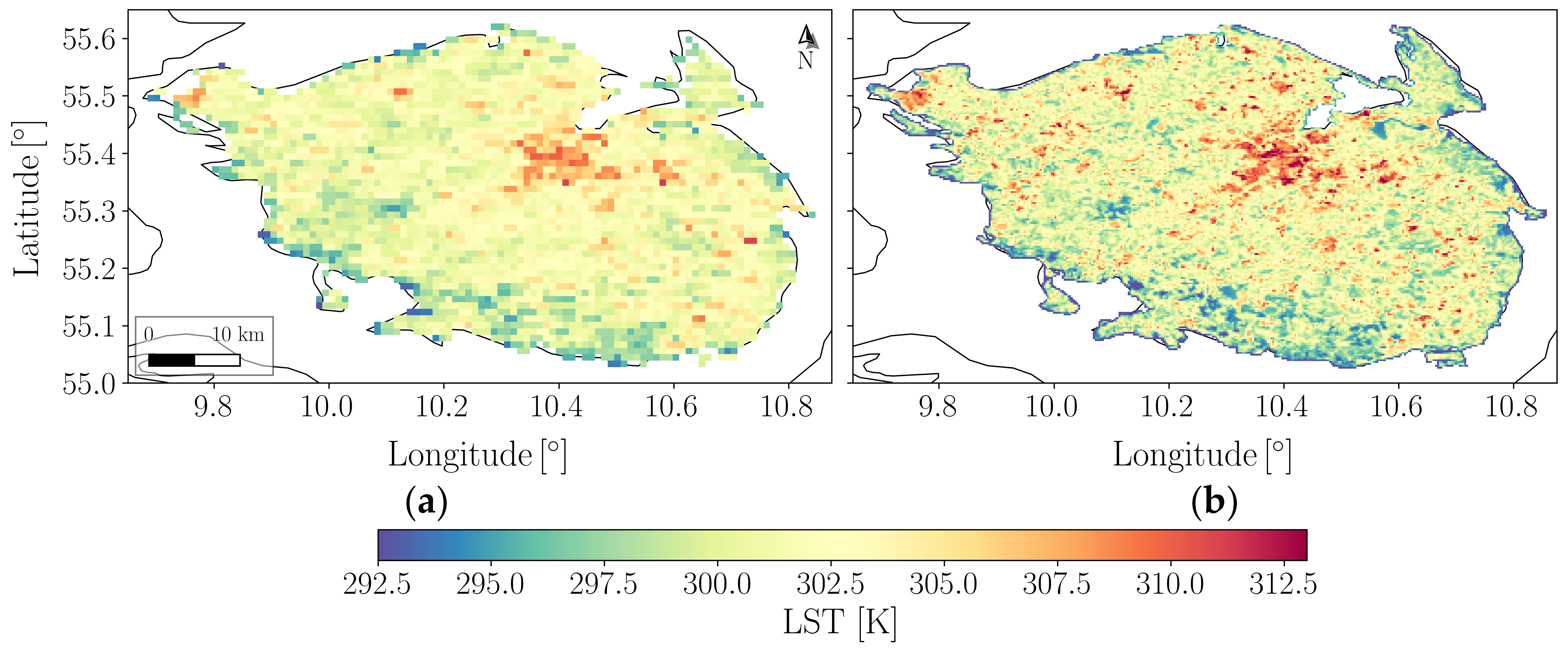
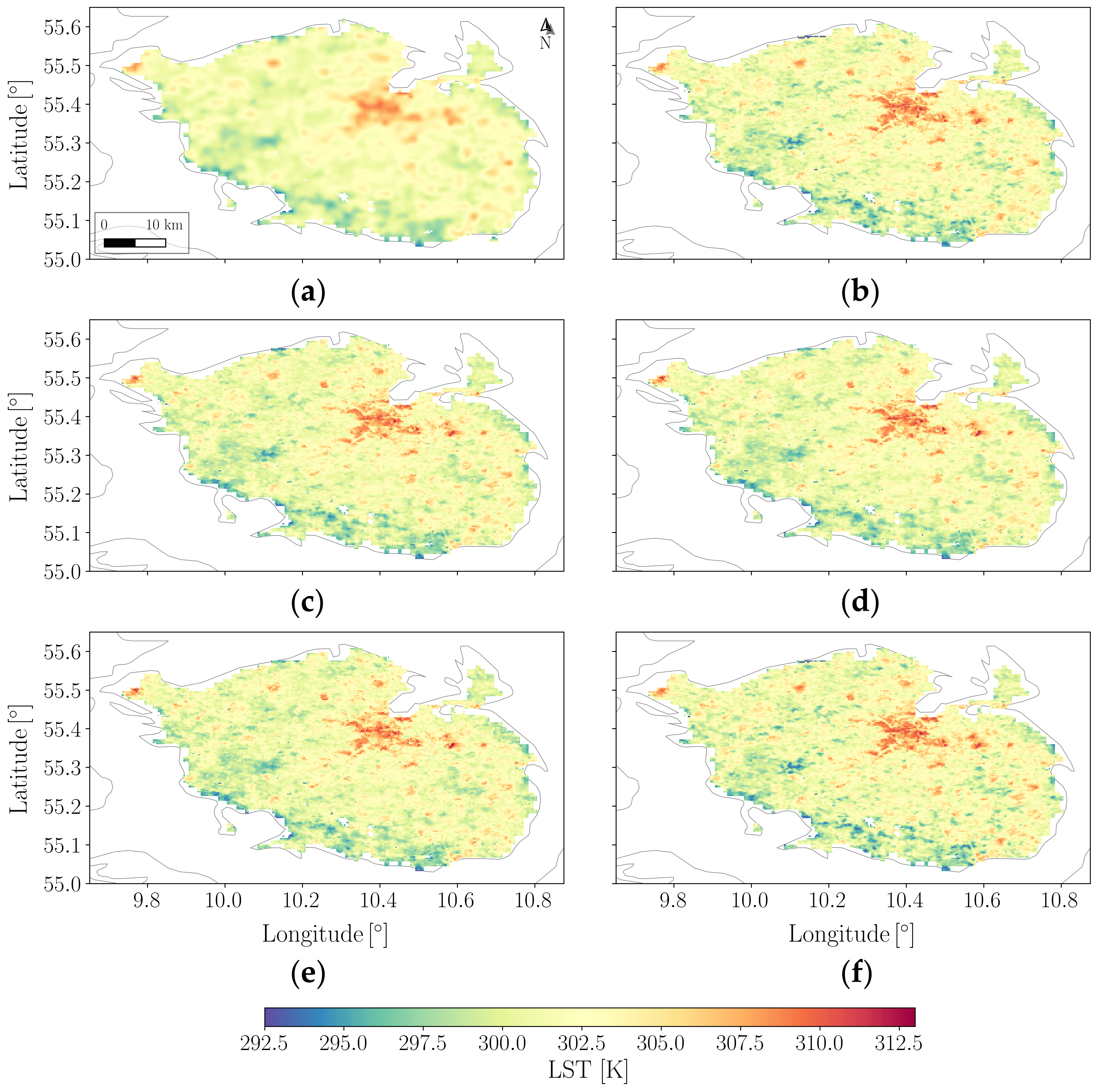
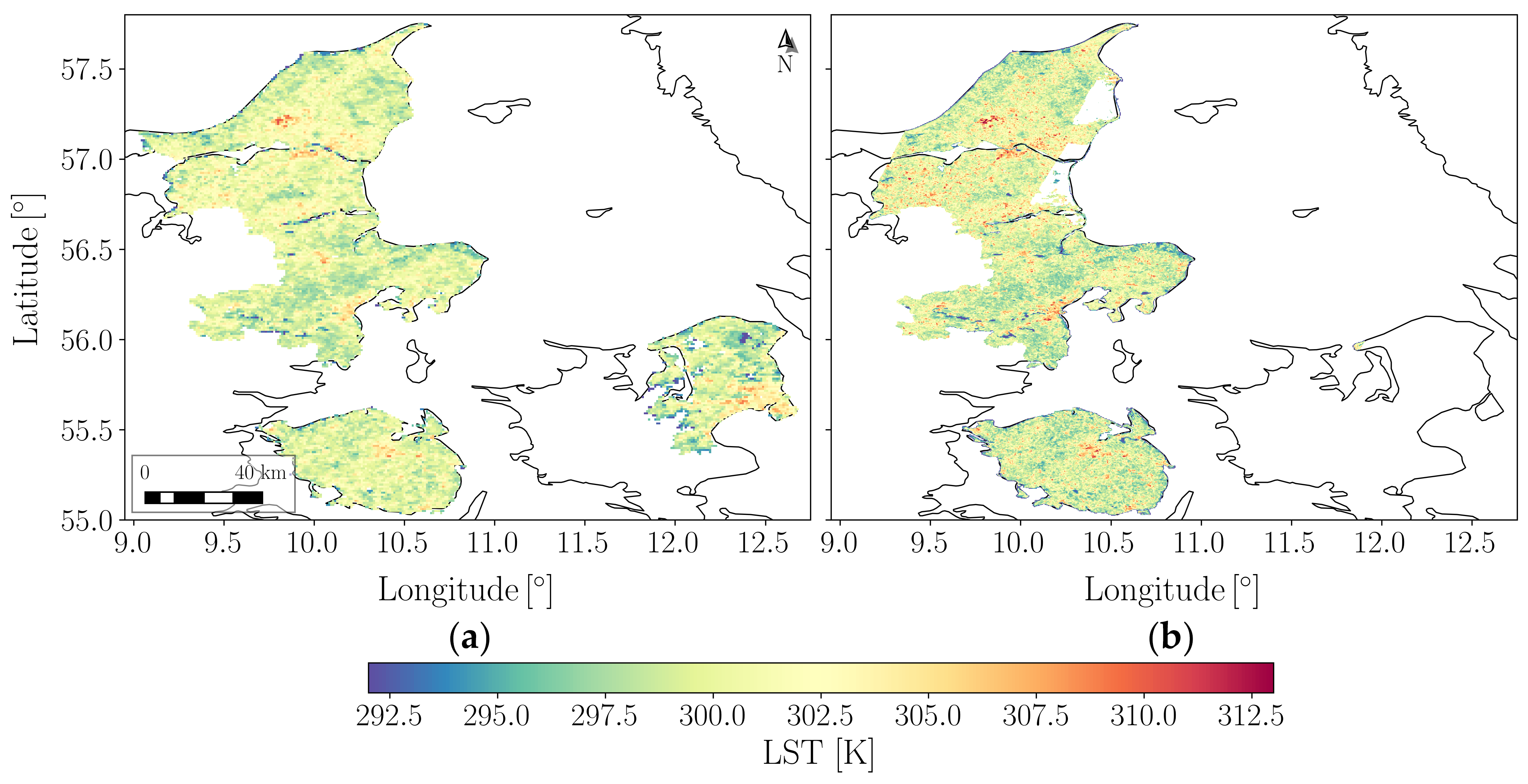
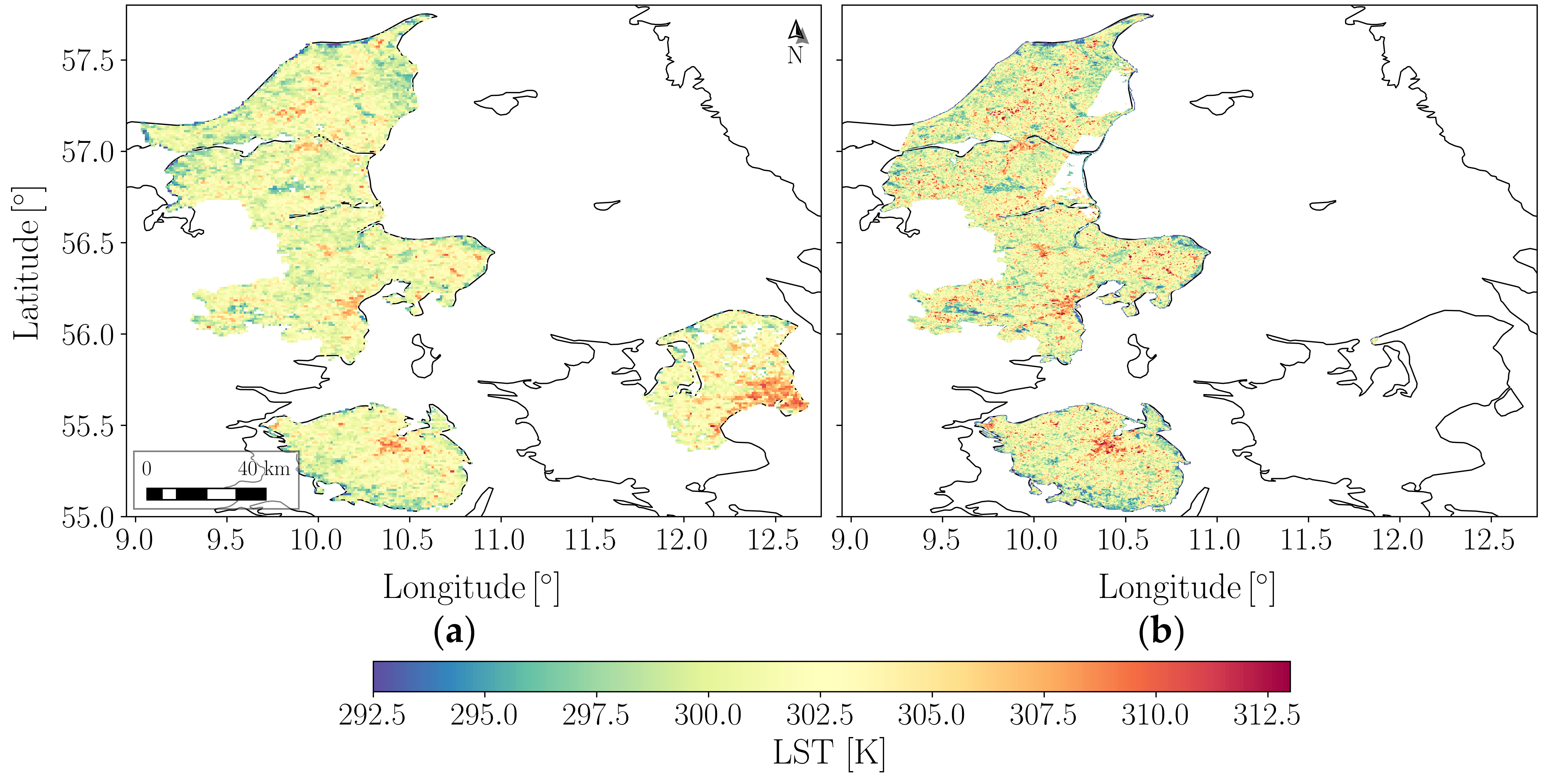
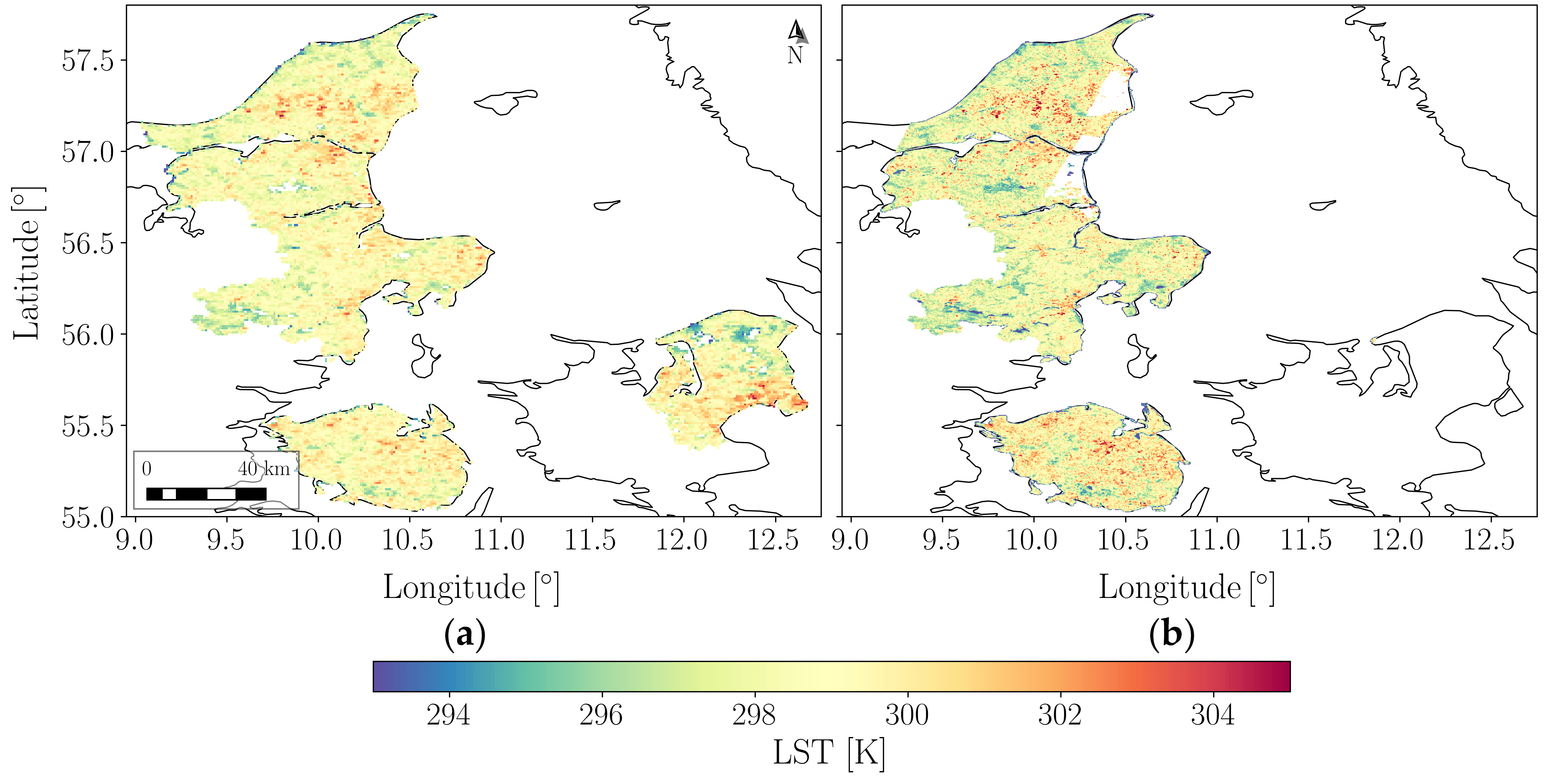
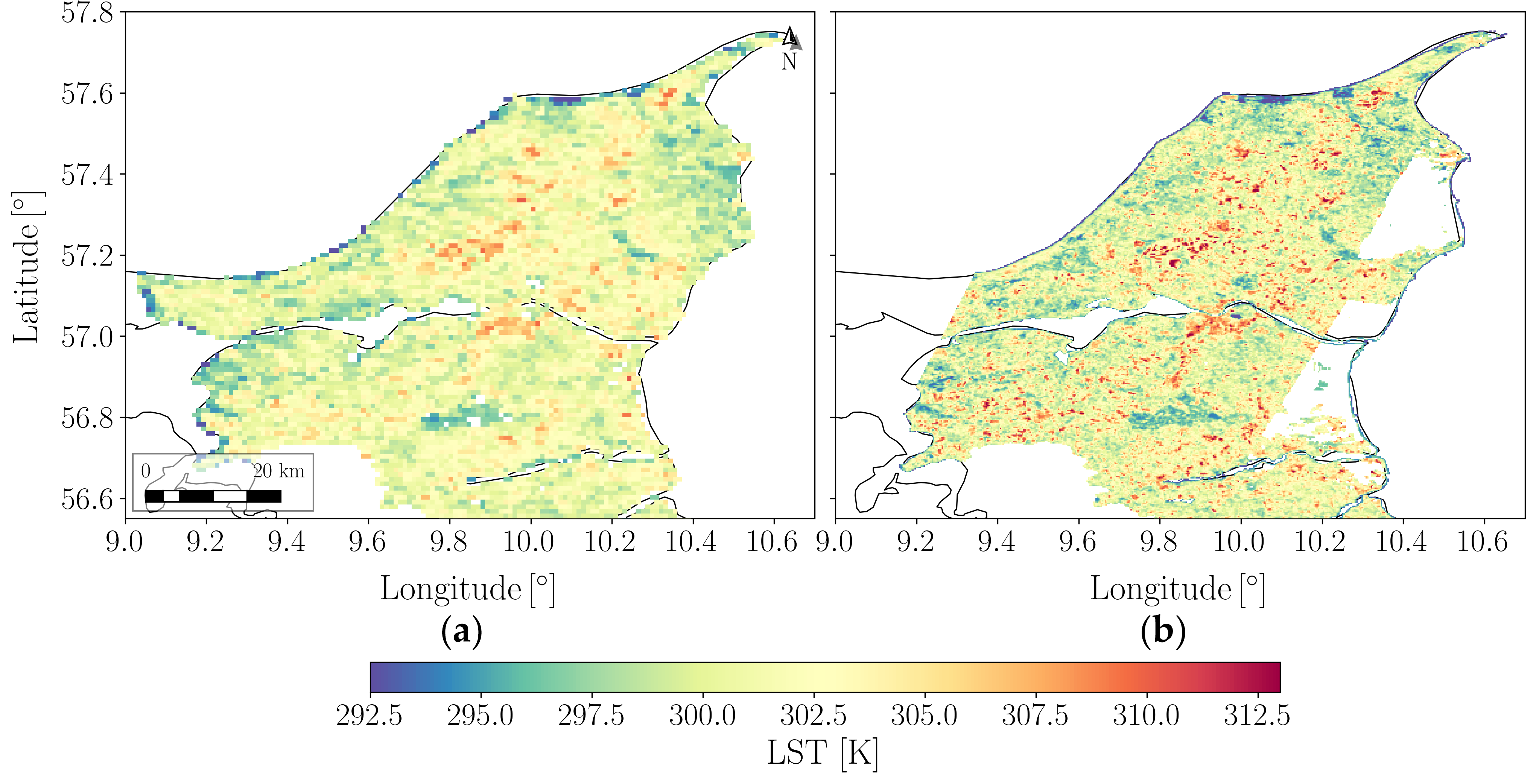
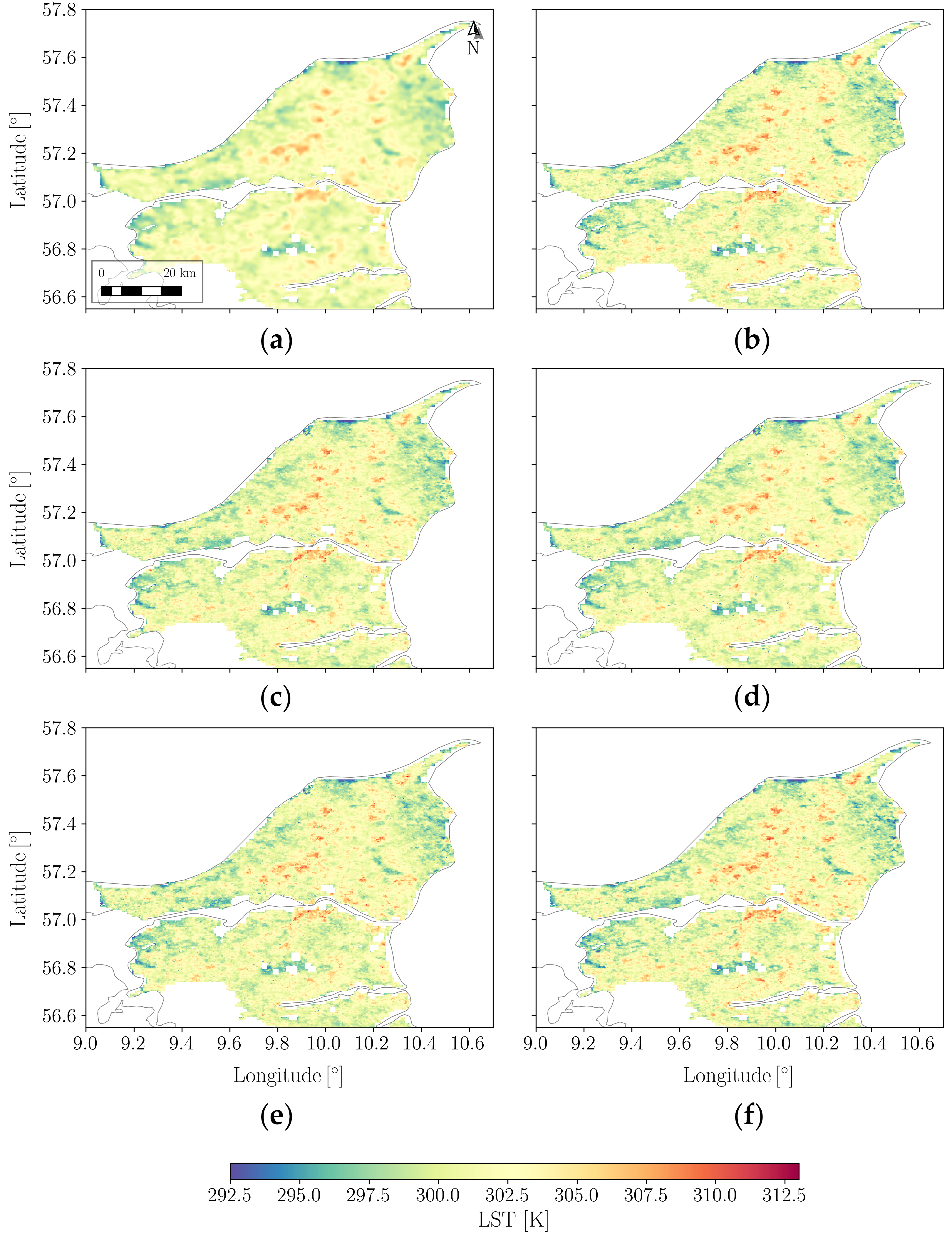
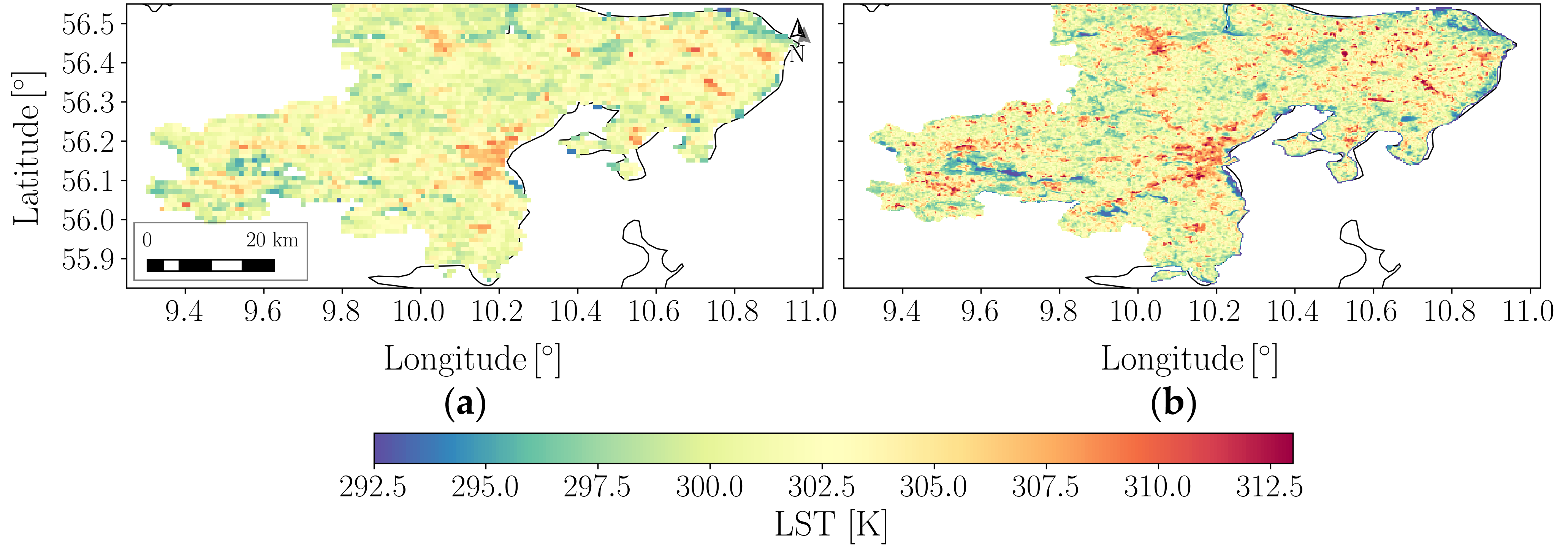
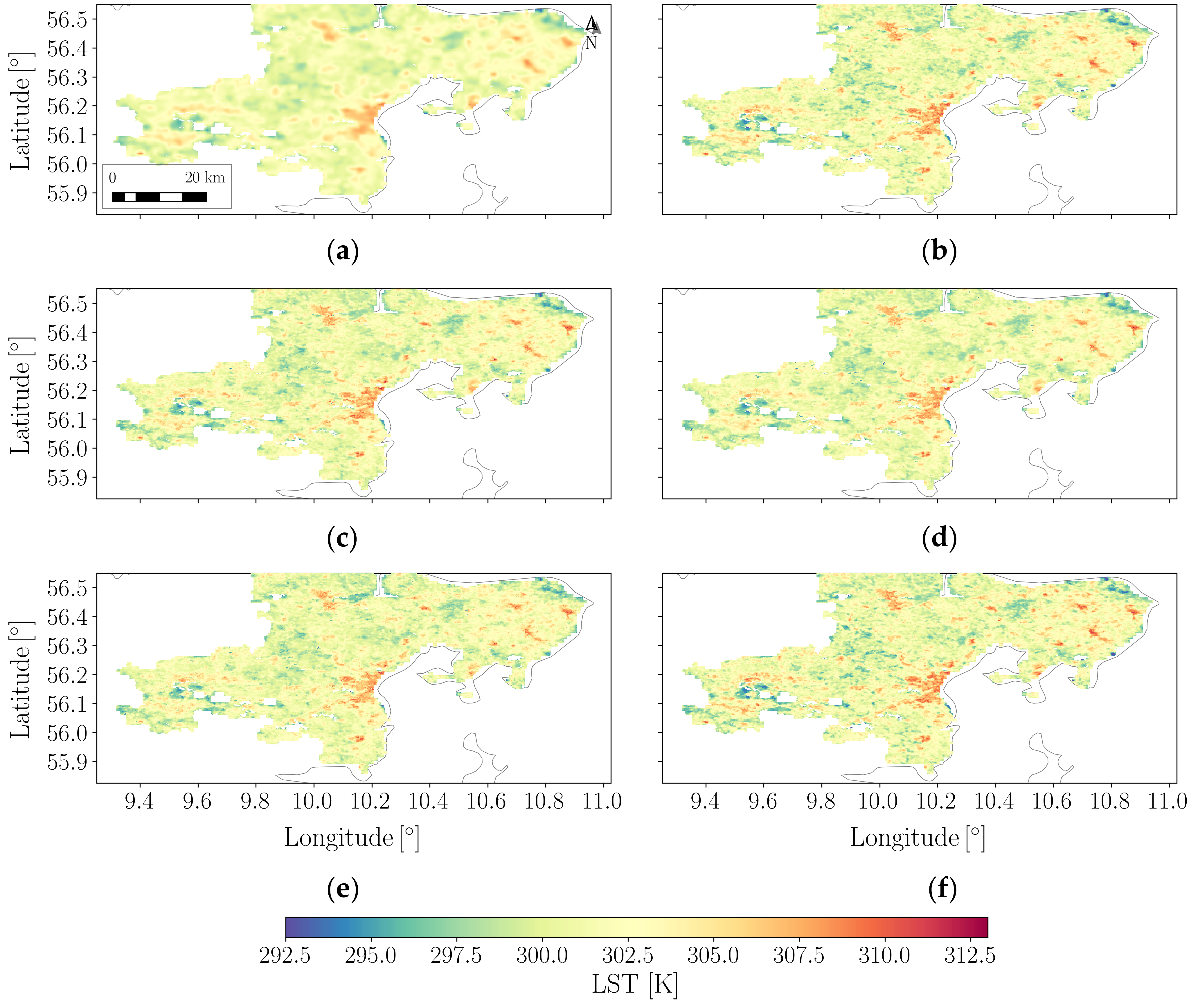
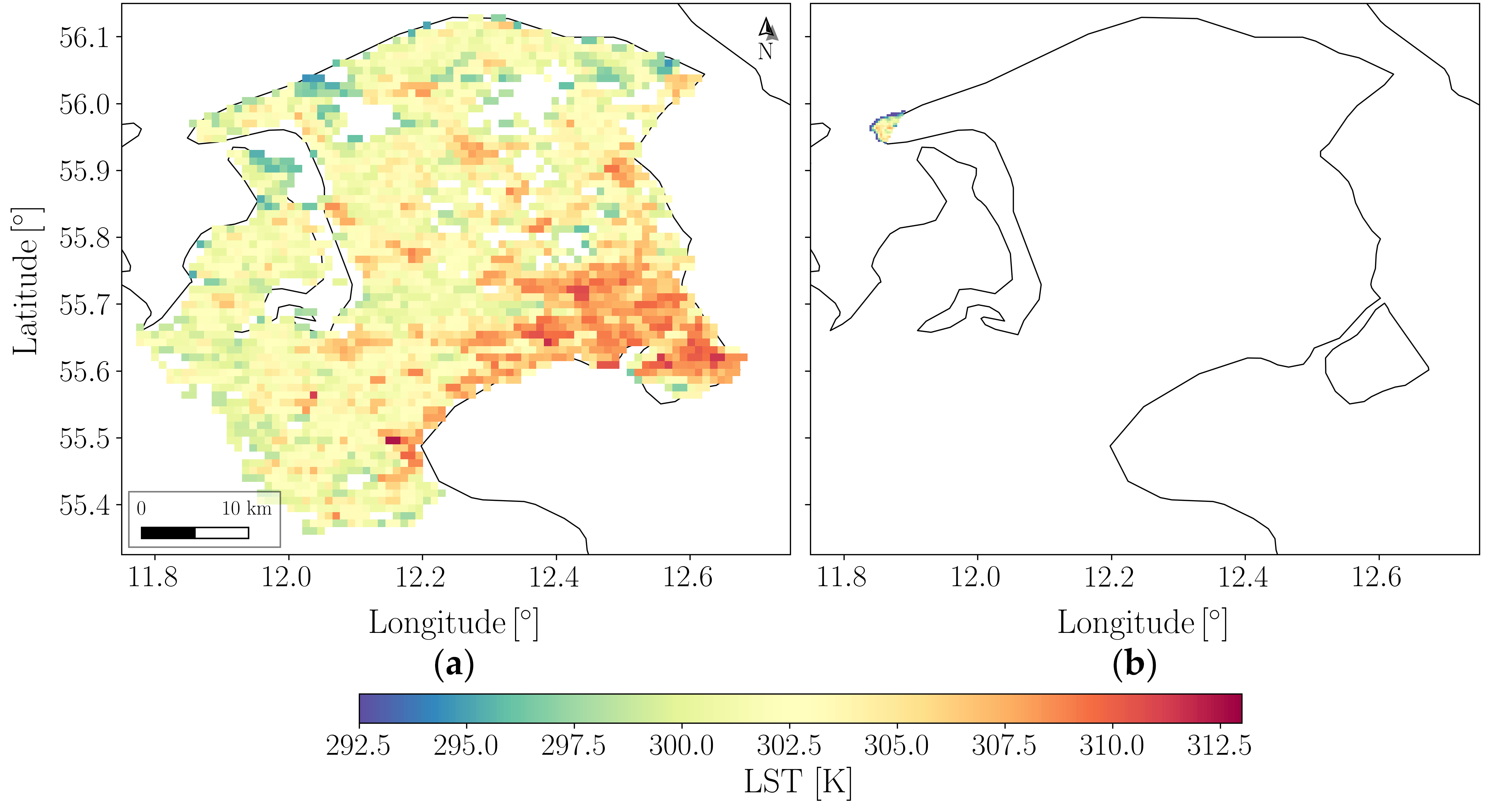
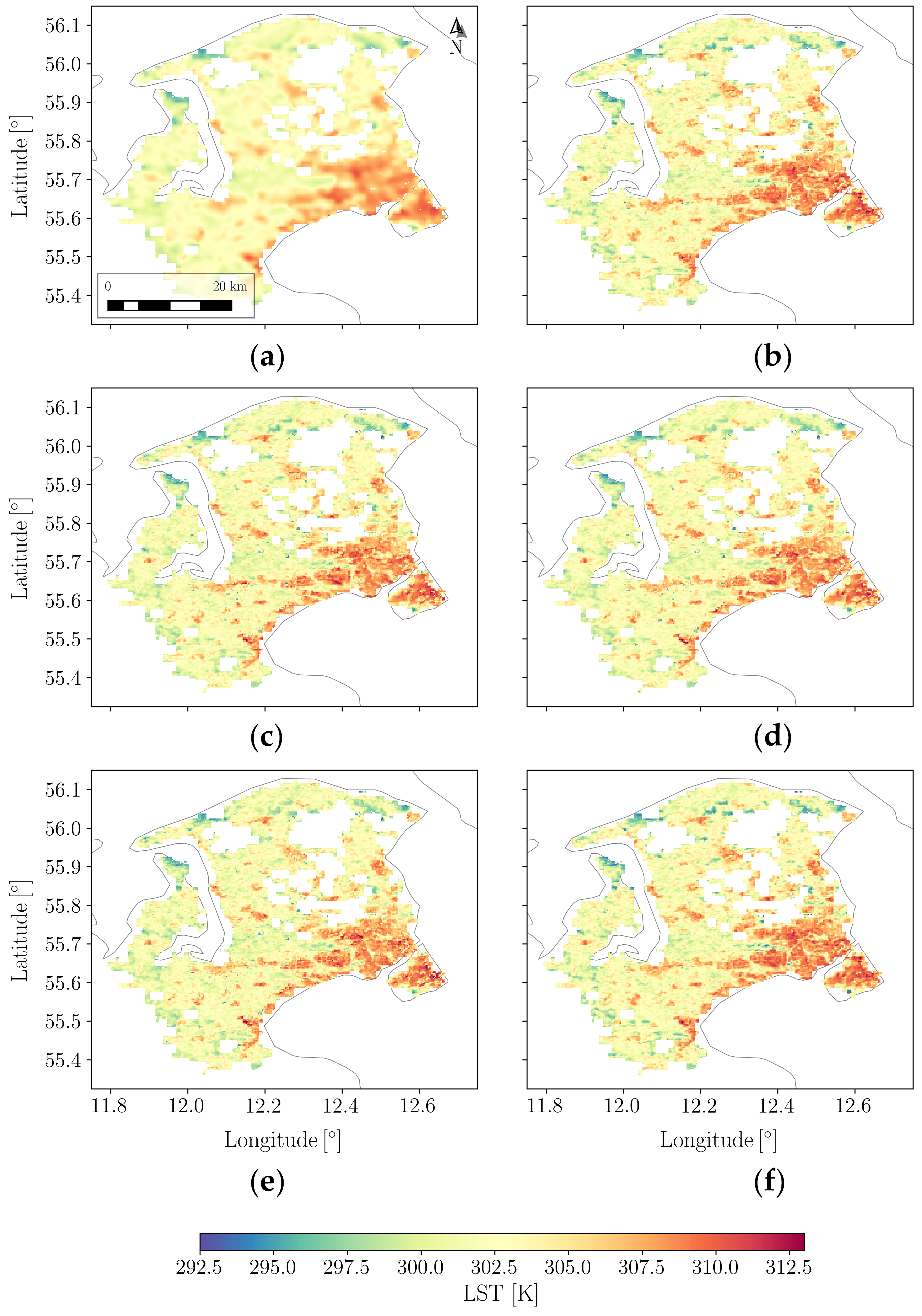
Due to the large extent of the AOI, a full visual comparison between the true and predicted LST maps would be unfeasible. A visual comparison may rather be done instead at an FUA level. Figure 27 presents the coarse Sentinel-3 and fine Landsat LST values for Odense on 8 June 2023 while Figure 28 presents the fine values predicted by the downscaling models considering residual correction. Analogous figures for all the other regions are found in Appendix A.3 (Figure A11, Figure A12, Figure A13, Figure A14, Figure A15 and Figure A16), whose remarks and conclusions could be said to be identical to the ones which are herein presented for Odense. To facilitate comparison, all maps of each region are classified and displayed using a common colour scale. Odense’s maps show that all predicted fine-resolution LST products (except the dummy model’s) approximately exhibit similar spatial patterns in terms of distribution, colour tones, and texture features associated with different land-cover types (e.g., urban areas, bare land, and vegetation) reasonably matching those observed in the Landsat-derived fine-resolution LST . However, Landsat’s extreme values do appear to be more extreme than the predicted ones, as previously revealed by the previous quantitative analyses.
Although all models substantially enhance the visual quality relative to the coarse-resolution LST by effectively reducing the mosaic (tiling) artifacts, the single-timestamp model visibly, but moderately, outperforms the others in capturing extreme high-temperature signals in urban areas as well as the lowest temperatures in the scene. This indicates that single-timestamp LR is more effective at highlighting thermal contrasts between land-cover features, making it particularly suitable for urban heat island analysis. These observations are consistent with the quantitative evaluation, in which the single-timestamp model achieves significantly lower errors in general and at the high extremes when compared to the other models.
Note that, despite the lowest LST values being consistently observed over water bodies in both the Landsat and Sentinel-3 LST products, these areas are absent from the predicted LST maps. This is due to the fact of the original Sentinel-3 SYN products (whose derived variables are used as predictors of the downscaling models) having their water pixels masked out.

3.9. Maps of the Downscaling Error

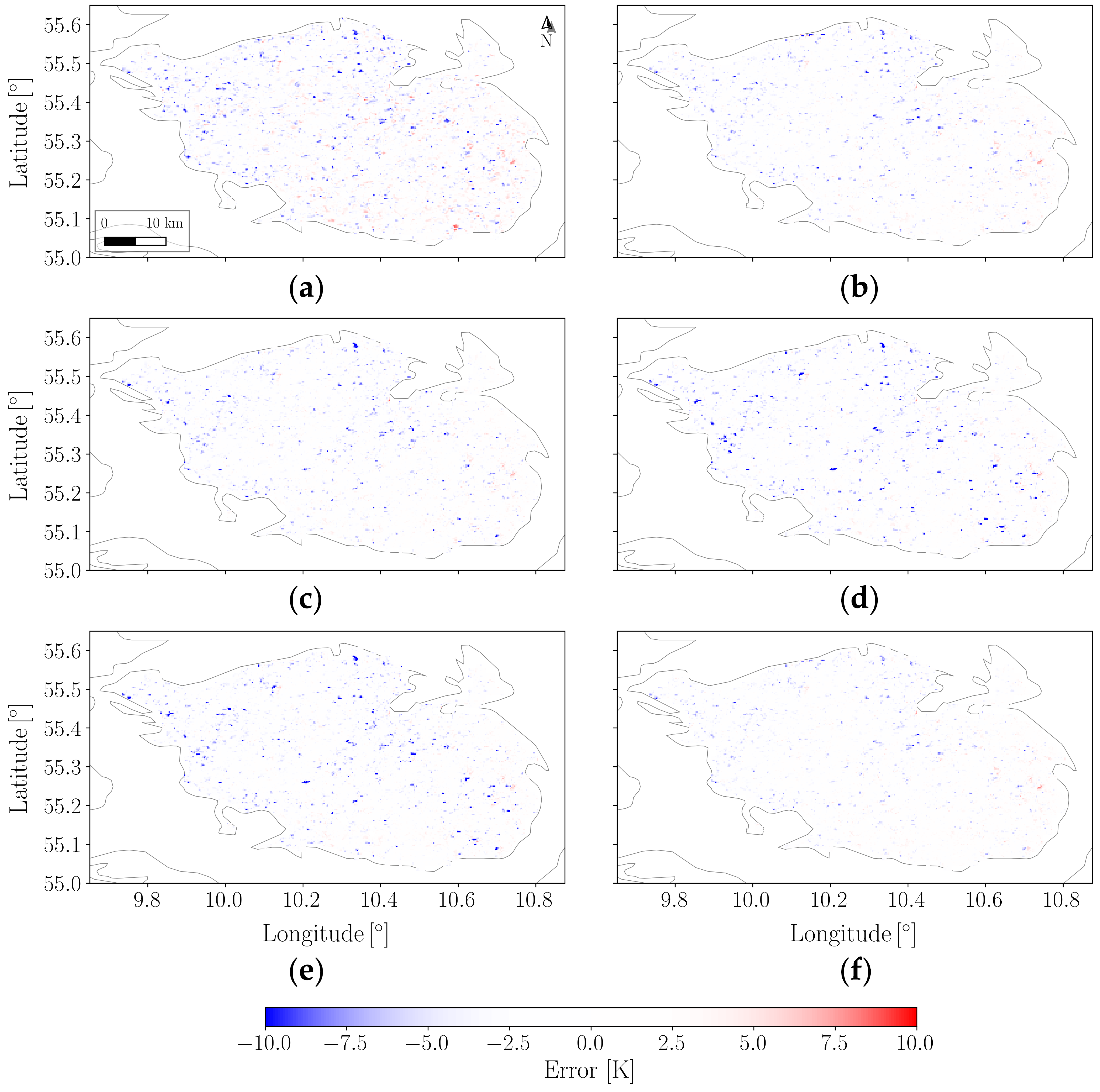
Figure 29 presents the error obtained by the downscaling models for Odense on 8 June 2023. One should note here that the colourmap limits were truncated to avoid presenting sparse outliers that would overwhelm the colour spectrum. Not surprisingly, the dummy model is the one with the highest amount of extreme error values when considering both lower and higher limits The tree-based models do evidence strong underestimation, presenting lower extreme errors that even surpass DMR’s. Also, single-timestamp LR is unequivocally found to be the model that produces the smallest amount of extreme errors.

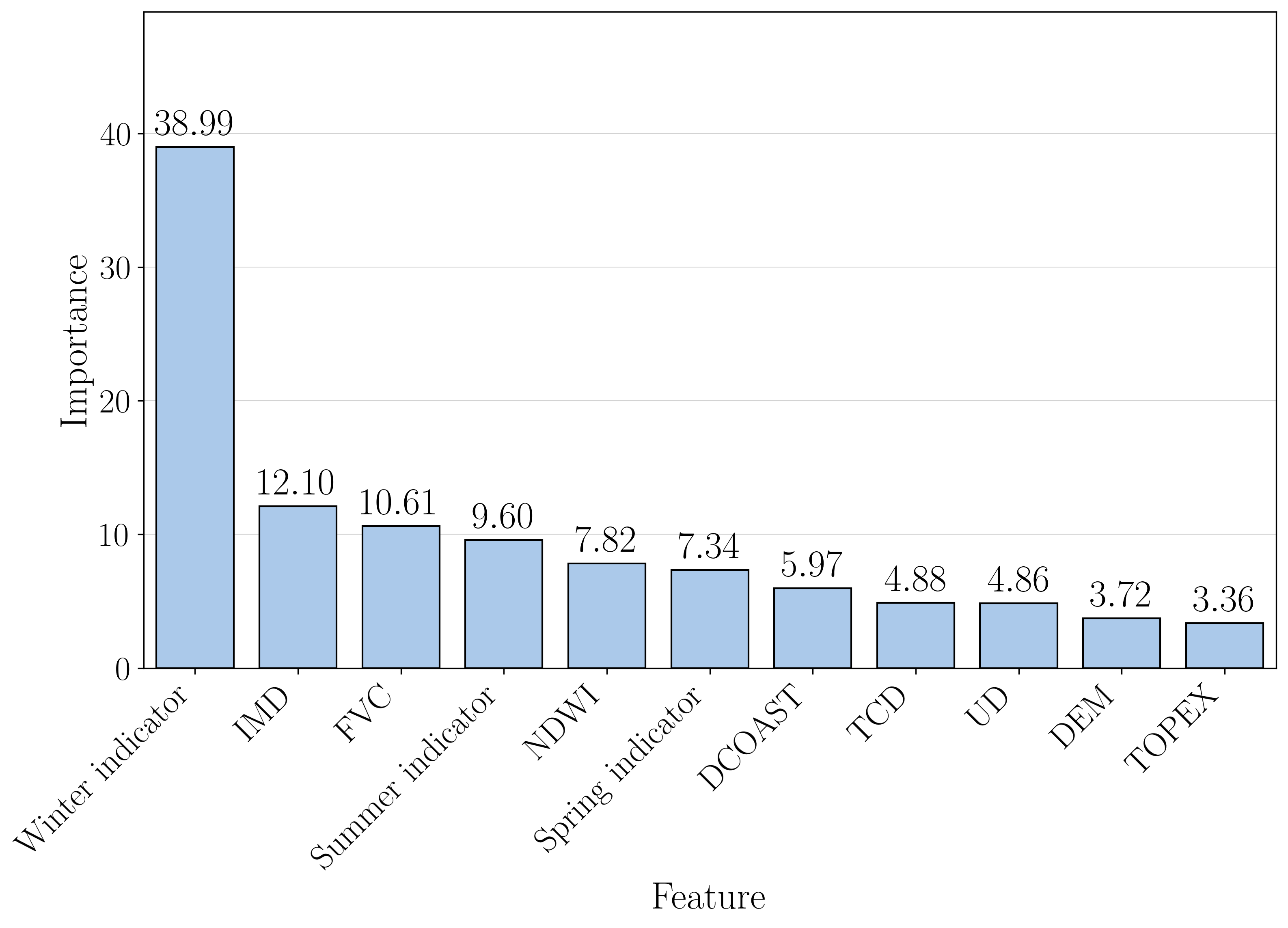
3.10. Feature Importance According to Best Coarse Predicting Model

The feature selection study which was previously performed with the multi-timestamp LR model gave a hint about the relative importance of each feature in a linear model for the relation between feature and target in the coarse grid. However, it would also be pertinent to numerically quantify these importances using the model that best captured the coarse relationship: the multi-timestamp GB model. Fortunately, the XGBoost package already provides a built-in function for computing such feature importances. In this work, feature importance was defined as the average information gain across all tree splits the feature is used in. Figure 30 shows that the most important features for MTS-GB were the winter season indicator (that is, whether the season corresponds to winter (returning 1 ) or not (returning 0 )), followed by IMD , FVC , summer season indicator NDWI , spring season indicator, DCOAST , TCD , UD , DEM and TOPEX . The curious reader may be intrigued by the non-consideration of an autumn season indicator as a feature of the GB model. One may show that the autumn season indicator is redundant with the presence of all other season indicators: if all the latter do not indicate the respective season, then autumn is necessarily the actual season. The drop of this feature was a direct consequence of the used dummy encoding in the preprocessing of the categorical variables within the downscaling pipeline.
The quite large value obtained for the winter season indicator evidences how the data associated with this season strongly differs from the data associated with all the others and how the inclusion of seasonality is remarkably important for the conception of a more accurate multi-timestamp ML model. The results of the previous feature selection study (using the MTS-LR model and presented in Table 3, whose outcomes for the NDVI predictor should in this comparison be disregarded due to its near-collinearity with FVC ) already emphasised the importance of FVC , IMD and NDWI , however, with a different order: in contrast with MTS-LR, MTS-GB gave more importance to IMD than to FVC. Nonetheless, MTS-LR and MTS-GB regarded the numerical predictors with strong similarity: either the numerical predictors remained in the same position (NDWI) or moved one (FVC, IMD, TCD, DCOAST, DEM and TOPEX) or two positions (UD).
The present results show how linear and non-linear models may give different importances to each predictor and that the best set according to one may not actually be the best according to another. Still, one should note that the results of the two analyses are not completely comparable since they rely on quite different feature importance quantification methods. The conclusions drawn from the present comparison should, therefore, be interpreted with caution.

4. Discussion

Numerous studies in the literature have discussed and benchmarked single-timestamp scale invariance models. However, studies addressing multi-timestamp models, such as the ones considered in this work, remain scarce. This has made the scrutiny of multi-timestamp models a difficult exercise within the current state of the art. Still, the results and learnings from other works regarding single-timestamp models can guide the judgement of all models employed in the present study.

4.1. Model Extrapolation and Breakage of Scale Invariance

Suboptimal performance of the ML models in fine-scale prediction when trained with coarse-scale data, as found in the present work, had been emphasised in other studies. Ding et al. [45] simulated coarse LST from Landsat fine data through weighted averaging and downscaled it with different single-timestamp models, one of them corresponding to RF. As in the present work, they did observe that RF could not predict the extremes of the original fine LST data due to the loss of such information when simulating the coarse data. They termed the phenomenon “boundary effect”. Hutengs and Vohland [25] also concluded from their work that “the inability to reproduce very high and very low temperatures is likely caused by an insufficient number of training samples in these temperature ranges”. Furthermore, the results of the experiment done by Hernanz et al. [87] on the extrapolation of NN and support vector regression models for the prediction of maximum surface temperature made them to state that the “ML techniques can perform wrong under extrapolation” and that “their suitability for SD of climate change projections should be seriously questioned”. They further mention that “experiments which validate over spatially/temporarily aggregated data might hide extrapolation problems in finer spatial/temporal scales”—as are the scale invariance architectures considered in the present work. Moreover, underperformance may additionally be exacerbated by the non-verification of the scale invariance principle. Gao et al. [81] concluded that, although “this assumption is reasonable for a uniformly (homogeneous) vegetated area and worked well in rainfed agricultural areas”, the “LST-NDVI relationship is not well-defined over many complex heterogeneous landscapes” as demonstrated in previous studies [34,80,88,89,90,91]. This is, in fact, also the case of the Danish functional urban areas considered in the present work, which are described by a large variety of LCZ classes (evidenced by Figure 6). Moreover, the present work indeed also revealed the worse downscaling metrics to occur for the timestamps whose validation domain included the highly urbanised area of Copenhagen.

4.2. Differences in the Native and Validation Remote Sensing Platforms

Strong evidence was found in the literature for the benchmarking results of the downscaling models being highly dependent on the LST coarse- and fine-resolution products (e.g., instruments, bands used, processing algorithm) employed in training and validation, respectively. Hutengs and Vohland [25] showed that, while RF was able to perform better than TsHARP when training with simulated coarse data from a validating fine Landsat one, it did it marginally when training with coarse MODIS data and validating with the same Landsat data. And it should be noted that, while RF used several predictors in the downscaling, TsHARP used solely one (FVC). The authors emphasised the fact that using coarsened and fine LST data from the same instrument for training and validation, respectively, was a “best case scenario”, which, in contrast to the case in which different instruments were used, did not suffer from mismatches in radiometric processing or geo-referencing (as well as acquisition time). Because of this, many downscaling models have been tested within such a framework [16,32,45,79,81]. However, one cannot guarantee that these models would perform identically well in practical downscaling applications which use a “real” coarse LST instead of a simulated one. In the case of using different training and validating instruments, and as previously concluded, the authors stated that the not much better results that they obtained when downscaling with an RF model in the place of TsHARP could be partially justified by the absence of extremes in the training coarse data (i.e., the MODIS LST values do not encompass the high extreme ones of Landsat). Because of this, the authors stated that “for RF regression (…) one has to be aware that the predictive range of LSTs is restricted to those covered by the training data”. With all these reflections, one may more confidently postulate that limitations of the downscaling performance of the models obtained in the present work could indeed be partially explained by the mismatch between the two instruments (and the different LST processing algorithms for each one) issuing the training and validating data. And this has been further emphasised by the discrepancies which were herein found, namely the not so large Pearson coefficient value of 0.79 between the Sentinel-3 and Landsat LST data in the coarse grid of the former, the respective non-negligible mean absolute difference of 0.98 K and the occurrence of large outliers in these differences. Indeed, with such a Pearson coefficient, R 2 scores not much larger than 0.62 could be expected from the downscaling results—as indeed observed in the present work.

4.3. Differences in Model Benchmarking Approaches Across the Literature

A vast amount of works report significant improvements when using a single-timestamp RF model in place of the ubiquitous TsHARP or DisTrad models. However, while these RF models employed multiple predictors, TsHARP and DisTrad solely regard one (FVC and NDVI, respectively), which would raise the question of whether such relative improvements can still occur if the multiple predictors were also used in an LR model. For instance, Pu [44] downscaled MODIS LST using a multivariate LR model and NN and validated the result with fine ASTER data which subsequently revealed NN to actually perform worse than LR. Moreover, one should take into account that this result is obtained for the advantageous case in which the native and validating sensors (MODIS and ASTER sensors) pertain to the same platform (Terra), making the samples concomitant and the discrepancies caused by geometric observation deviations negligible [41]. Also, most works issue general scores for the downscaling of the whole data, but not particular ones for the data extremes (which are notably important in the context of urban planning). Works such as the ones of Li et al. [47] and Wu and Li [41], who downscaled coarse MODIS LST and validated the result with fine ASTER data, showed that the single-timestamp RF model can perform, overall, significantly better than TsHARP. However, the resultant maps revealed that, in contrast with TsHARP, RF could not predict the low and high extremes of the true fine LST . Moreover, Wu and Li [41] showed that, for impervious surfaces, which usually contain the highest LST values in the scene, a multiple-predictor RF model may perform even worse than the single-predictor TsHARP model. These findings suggest that underperformance of the tree-based models in the extremes, as observed in the present work, is a common limitation of this type or architecture.

4.4. Possible Solutions to Model Extrapolation and Breakage of Scale Invariance

Wang et al. [43] considered LST data simulation in their downscaling models: instead of the ubiquitous direct weighted spatial average, the authors employed a Planck’s law-based method to obtain training coarse LST data from a validating fine Landsat one. This method seems to conserve much more the extremes of the fine data than the traditional one, as presented by the resultant maps shown in their work. Subsequently, the trained tree-based models were found not to suffer from the “boundary effect” and were able to predict the tails of the fine LST distribution. However, one should point out that, for the case of the coarsening of Landsat-derived predictors, the traditional weighted spatial average was the method used, which could create a mismatch between the predictor and target value distributions—something that merits future study. The authors revealed that all ML models performed better than the LR ones, though, again, by considering multiple predictors for the former and just one for the latter (since TsHARP and DisTrad were tried). Nonetheless, even though the LST coarsening method employed by the authors can only make sense in the realm of LST data simulations, it may motivate one to consider identical approaches for “real” world practices, and this does not only include transformations of the coarse data but also data augmentations.
The literature reveals that another modification that could mitigate the extrapolation is the consideration of a step-by-step (also termed “stepwise”) approach while assuming scale invariance between each successive scale. Instead of directly downscaling from native to target scale, the stepwise approach employs a scale-invariance-based downscaling model between native and an in-between scale and another between the latter and a successively smaller scale (trained with the data produced by the previous step) until the target scale is reached [33,92]. As in the present work, Li et al. [33] downscaled Sentinel-3 LST and validated the result with Landsat-8 data (however, using Sentinel-2-derived spectral indices as predictors instead of Sentinel-3 SYN’s). The employment of a direct and stepwise scale-invariance-based downscaler using RF as a base model revealed that the latter, in contrast with the former, was able to approximately attain the extremes of the validation data and to produce a much smaller downscaling error. Such results strongly encourage the usage of the stepwise approach in place of the direct one.
To overcome the issue of scale invariance breakage, an approach such as the one implemented by Ait-Bachir et al. [70], which does not rely on that principle, could be considered. The strategy regarded by the authors consisted in the interpolation of coarse LST onto the fine grid and training of a model that predicts a fine target with it as well as fine NDVI so that the degradation of the prediction (onto the coarse grid) gets as close as possible to the original coarse LST . Note that this, however, relies on another hypothesis: that the inverse transformation of the coarsening of the predicted fine target concomitantly also gets as close as possible to the true fine LST data. Indeed, coarsening results in loss of information, and one may show that it is possible for the degradations of different fine scenes to result in a common coarse scene—the inverse transformation can then have multiple solutions. This means that, even though the degraded predicted target can get close enough to the true coarse one, the predicted fine target can only get close to the true fine one within some irreducible tolerance.
All of these approaches are candidate topics for future work.

4.5. A Note on Model Transferability

The exploratory Pearson correlation study presented in this work revealed that single-timestamp models do underperform when inferring for non-training timestamps. Fortunately, preservation of predictor–target correlation within each one may be approximately achieved by considering timestamp-specific standardisation of the spatio-temporal variables as herein done for the case of the multi-timestamp models. While standardised multi-timestamp models may allow inter-timestamp transferability, their inter-space and inter-platform transferabilities could still be comparable to those of the single-timestamp models.
Additional questions also arise regarding the varying importance of features across different regions. For instance, in landlocked inland areas—unlike coastal regions—distance to coast is often largely irrelevant. In these cases, alternative predictors such as a digital elevation model may exhibit a comparable relationship with LST and could provide a more robust choice when spatial generalisability is desired. And because digital elevation models and distance to coast are strongly correlated with each other in coastal areas, the former may be used as a proxy for the latter for that case too.
To properly describe models’ transferability, these points should be thoroughly addressed.

5. Conclusions

The primary objective of this study was to assess whether the employment of practical ML models can provide better results than LR in a downscaling pipeline based on the scale invariance principle and residual correction. To do this, multi-timestamp ML models were benchmarked against a single-timestamp LR alternative. The performed exploratory data analysis revealed that, to preserve the strong within-timestamp correlation of the spatio-temporal predictors ( FVC , NDVI and NDWI ), the multi-timestamp models would need to be trained to infer for a standardised LST using also standardised spatio-temporal predictors. The subsequent tuning, training and testing of the resultant models revealed that the multi-timestamp architecture is able to achieve better results for coarse prediction than the single-timestamp one when using ML-based models. This demonstrates that ML models can outperform LR in the inference of a target with the same resolution as the training one. And the very same conclusions were reached when considering Landsat’s coarsened LST as a true target.
Regarding fine predictions without residual correction, all scores got significantly worse than in coarse prediction for the case of the ML models, which evidences breakage of scale invariance. GB and RF herein corresponded to the worst fine predicting models. As found in previous works, the suboptimal performance of the tree-based models could be justified by the so-called “boundary effect”, in which the absence of the fine extremes in the training coarse data makes the downscaling models extrapolate in fine prediction. In such conditions the tree-based models tend to behave poorly. Moreover, breakage of scale invariance and a stronger specificity of the ML models towards the training scale may make them overfit and perform significantly worse in a different scale. When considering residual correction, all produced RMSE values abruptly decreased. However, the single-timestamp model remained, overall, the best model and all ML models ceased to outperform the multi-timestamp LR one.
The present work also revealed that training with data from multiple timestamps instead of from solely one may actually deteriorate performance of the downscaling models, as common generalities (averages) between the different timestamps tend to be more emphasised than their particularities (extremes). This is evidenced by the greater capacity for the single-timestamp model to predict the tails of the fine target value distribution when compared to the other models and the fact that it was also able to outperform its multi-timestamp counterpart (LR) in all the considered test cases.
The present study demonstrated that, in the realm of scale-invariance-based models, the simplicity and overall better performance of the single-timestamp LR position it as the best candidate for operational LST downscaling applications.

Author Contributions

Conceptualization, É.P. and M.K.; methodology, É.P., M.K. and Q.P.; software, É.P. and M.K.; validation, É.P. and M.K.; formal analysis, É.P. and M.K.; data curation, I.G. and B.M.; writing—original draft preparation, É.P.; writing—review and editing, É.P., I.G., V.F.V.V.d.M., H.J.D.S., Q.P. and A.O.; visualization, É.P. and M.K.; supervision, A.O.; project administration, H.J.D.S., Q.P. and A.O.; funding acquisition, H.J.D.S. and A.O. All authors have read and agreed to the published version of the manuscript.

Funding

This research was funded by the European Space Agency (ESA) under Contract No. 4000143628/24/I-DT (AI Trustworthy Applications for Climate). This work was also supported by the Recovery and Resilience Plan Investment RE-C05-i02: Interface Mission—CoLAB, certified by the National Innovation Agency (Project N.º 01/C05-i02/2022).

Data Availability Statement

The downscaled LST data produced in this study using the benchmarking single-timestamp LR model are openly available in Zenodo at: https://doi.org/10.5281/zenodo.20863040 (accessed on 25 June 2026). Note that this repository further provides counterpart upsampled LST data produced using pure interpolation and the Landsat LST processed products (in their original resolution) which were herein employed in the validation of the tuned models. Additionally, test scores for coarse and fine prediction are issued for both downscaling and interpolation models.

Acknowledgments

This activity was carried out in the context of the CLIM4cities project, led by the Danish Meteorological Institute (DMI) in collaboration with +ATLANTIC CoLAB. The authors gratefully acknowledge the support and guidance of the ESA Φ-lab and Climate Office throughout this work. The views expressed in this publication are those of the authors and do not reflect the official opinion of the European Space Agency. This publication has been prepared using European Union’s Copernicus Land Monitoring Service information; https://doi.org/10.2909/fb4dffa1-6ceb-4cc0-8372-1ed354c285e6 (Urban Atlas 2018), https://doi.org/10.2909/3bf542bd-eebd-4d73-b53c-a0243f2ed862 (Imperviousness Density 2018—10 m), https://doi.org/10.2909/e677441e-fb94-431c-b4f9-304f10e4dfd8 (Tree Cover Density 2018—10 m), https://doi.org/10.2909/82f93572-9888-47ef-97a1-5cac5985a26a (Dominant Leaf Type 2018), https://doi.org/10.2909/0b6254bb-4c7d-41d9-8eae-c43b05ab2965 (Grasslands 2018—raster 10 m), https://doi.org/10.2909/71c95a07-e296-44fc-b22b-415f42acfdf0 (Corine Land Cover 2018—raster) (all accessed on 22 July 2024).

Conflicts of Interest

The authors declare no conflicts of interest. A scientific employee of the funding body took part in analysing and interpreting the results, as well as in reviewing the manuscript.

Correction Statement

This article has been republished with a minor correction to the image quality of all figures. This change does not affect the scientific content of the article.

Appendix A

Appendix A.1

  • Unique identifiers of the matched satellite products
Table A1. Unique identifiers of satellite imagery of the matching dates between Sentinel-3 and Landsat 8/9.
Sentinel-3Landsat 8/9
S3A_SL_2_LST____20200530T101738_20200530T102038_20200531T155247_0180_059_008_1980_LN2_O_NT_004.SEN3LC08_L2SP_196020_20200530_20200820_02_T1
LC08_L2SP_196021_20200530_20200820_02_T1
S3A_SL_2_LST____20200615T100239_20200615T100539_20200616T162427_0179_059_236_1980_LN2_O_NT_004.SEN3LC08_L2SP_196020_20200615_20200823_02_T1
LC08_L2SP_196021_20200615_20200823_02_T1
S3B_SL_2_LST____20220419T101543_20220419T101843_20220420T063118_0179_065_065_1980_PS2_O_NT_004.SEN3LC09_L2SP_195021_20220419_20230421_02_T1
LC09_L2SP_195022_20220419_20230421_02_T1
S3A_SY_2_SYN____20221019T101010_20221019T101310_20221021T074604_0180_091_122_1980_PS1_O_NT_002.SEN3LC09_L2SP_196020_20221019_20230325_02_T1
LC09_L2SP_196021_20221019_20230325_02_T1
S3A_SL_2_LST____20230508T095900_20230508T100200_20230509T191603_0180_098_293_1980_PS1_O_NT_004.SEN3LC09_L2SP_195021_20230508_20230510_02_T1
LC09_L2SP_195022_20230508_20230510_02_T1
S3A_SL_2_LST____20230608T095513_20230608T095813_20230609T190024_0179_099_350_1980_PS1_O_NT_004.SEN3LC08_L2SP_196020_20230608_20230614_02_T1
LC08_L2SP_196021_20230608_20230614_02_T1
S3A_SL_2_LST____20230904T101349_20230904T101649_20230905T191154_0180_103_065_1980_PS1_O_NT_004.SEN3LC09_L2SP_196020_20230904_20230906_02_T1
LC09_L2SP_196021_20230904_20230906_02_T1

Appendix A.2

  • Timestamp-specific centring in a single-predictor LR model
Timestamp-specific centring in an LR model considering FVC as sole predictor would be such that the LST value at some timestamp t and some pixel is related to the respective FVC value—let these be denoted by LST t and FVC t —through
LST t LST - t = : Δ LST t = a FVC t FVC - t = : Δ FVC t + b ,
where LST - t and FVC - t correspond to the spatial arithmetic means of LST and FVC at timestamp t and a and b are the parameters of the LR model. Let Δ LST t and Δ FVC t denote the timestamp-specific centred LST and FVC values, respectively, for timestamp t . If Δ LST t was plotted against Δ FVC t , the value distributions for each timestamp would be centred (vertically and horizontally) at the origin.
  • Timestamp-specific standardisation in a single-predictor LR model
Timestamp-specific standardisation in an LR model considering FVC as sole predictor would be such that the LST value at some timestamp t and some pixel is related to the respective FVC value through
LST t LST - t s LST t = : δ LST t = a FVC t FVC - t s FVC t = : δ FVC t + b .
where s LST t and s FVC t are the sample standard deviations of the LST and FVC values for timestamp t .
Let δ LST t and δ FVC t denote the timestamp-specific standardised LST and FVC values for timestamp t .
  • Similarity between a multi-timestamp single-predictor LR model when considering timestamp-specific standardisation and a single-timestamp single-predictor LR model
A multi-timestamp LR model considering FVC as sole predictor with timestamp-specific standardisation would be equivalent to a single-timestamp one if the actual LST data were perfectly linear with respect to FVC and the line slopes of the raw data all had the same sign for all timestamps. Indeed, the solution of an LR problem using the raw data of a sole timestamp t may be shown to correspond to
δ LST t = R t δ FVC t ,
where R t is the Pearson correlation coefficient between LST and FVC values at that timestamp. If the raw data were perfectly linear for all timestamps and all line slopes shared the same sign, one would expect values of R t = 1 if the slopes were positive or R t = 1 if the slopes were negative. On the other hand, if δ LST t was plotted against δ FVC t for all timestamps, the resultant lines would be centred at the origin—implying b = 0 in (A2) (as in (A3))—and because in the case of perfect linearity the line slopes of the raw data coincide with R t s LST t / s FVC t , the line slopes of the standardised data would correspond to R t —implying a = R t in (A2) (as in (A3)).
  • Proof that, when residual correction is considered and the residual refinement is done through a linear operating interpolation method, a scale-invariance-based downscaling model whose base model predicts a constant c is equivalent to pure interpolation
According to the flow chart of Figure 5,
LST ^ fine ,   corr = δ LST ^ fine = c + ε ^ fine S LST coarse + LST - coarse ,   i   = c + interp fine ε coarse S LST coarse + LST - coarse   = c + interp fine δ LST coarse δ LST ^ coarse = c S LST coarse + LST - coarse   = c + interp fine LST coarse LST - coarse S LST coarse c S LST coarse + LST - coarse   = c c + interp fine ( LST coarse ) LST - coarse S LST coarse S LST coarse + LST - coarse   = interp fine ( LST coarse ) LST - coarse + LST - coarse   = interp fine ( LST coarse ) .
In the mathematical proof above, it is assumed that the interpolator for the refinement of the residuals is a linear operator (e.g., bilinear interpolation, cubic interpolation, cubic spline), therefore having the homogeneity property (the interpolation of a map multiplied by some factor is this factor multiplied the interpolation of the map) and addition property (the interpolation of the sum of maps is the sum of the interpolations of the maps).

Appendix A.3

  • Counterpart scatter plots of kernel density estimate representations
Figure A1. Predicted (straight lines) and actual (stains) coarse Sentinel-3’s LSTs without timestamp-specific transformation (left-hand side, (a)), with centring (centre, (b)) and with standardisation (right-hand side, (c)) for test timestamps. Prediction is done using a multi-timestamp LR model with FVC as predictor. This is a scatter plot associated with the kernel density estimate plot of Figure 9.
Remotesensing 18 02263 g0a1
Figure A2. Predicted versus actual fine LST with residual correction using the single-timestamp LR model for each test timestamp: 30 May 2020 (a), 15 June 2020 (b), 19 April 2022 (c), 19 October 2022 (d), 8 May 2023 (e), 8 June 2023 (f) and 4 September 2023 (g). The data is hued by Local Climate Zone ( LCZ ). This is a scatter plot associated with the kernel density estimate plot of Figure 20.
Remotesensing 18 02263 g0a2
Figure A3. Predicted versus actual fine LST with residual correction using the multi-timestamp NN model for each test timestamp: 30 May 2020 (a), 15 June 2020 (b), 19 April 2022 (c), 19 October 2022 (d), 8 May 2023 (e), 8 June 2023 (f) and 4 September 2023 (g). The data is hued by Local Climate Zone ( LCZ ). This is a scatter plot associated with the kernel density estimate plot of Figure 21.
Remotesensing 18 02263 g0a3
  • True LST maps for the whole AOI
Figure A4. Sentinel-3 coarse (a) and Landsat fine (b) LSTs for the whole AOI on 30 May 2020. Note that Landsat’s fine data corresponds to the original data reprojected to Sentinel-3’s fine grid.
Remotesensing 18 02263 g0a4
Figure A5. Sentinel-3 coarse (a) and Landsat fine (b) LSTs for the whole AOI on 15 June 2020. Note that Landsat’s fine data corresponds to the original data reprojected to Sentinel-3’s fine grid.
Remotesensing 18 02263 g0a5
Figure A6. Sentinel-3 coarse (a) and Landsat fine (b) LSTs for the whole AOI on 19 April 2022. Note that Landsat’s fine data corresponds to the original data reprojected to Sentinel-3’s fine grid.
Remotesensing 18 02263 g0a6
Figure A7. Sentinel-3 coarse (a) and Landsat fine (b) LSTs for the whole AOI on 19 October 2022. Note that Landsat’s fine data corresponds to the original data reprojected to Sentinel-3’s fine grid.
Remotesensing 18 02263 g0a7
Figure A8. Sentinel-3 coarse (a) and Landsat fine (b) LSTs for the whole AOI on 8 May 2023. Note that Landsat’s fine data corresponds to the original data reprojected to Sentinel-3’s fine grid.
Remotesensing 18 02263 g0a8
Figure A9. Sentinel-3 coarse (a) and Landsat fine (b) LSTs for the whole AOI on 8 June 2023. Note that Landsat’s fine data corresponds to the original data reprojected to Sentinel-3’s fine grid.
Remotesensing 18 02263 g0a9
Figure A10. Sentinel-3 coarse (a) and Landsat fine (b) LSTs for the whole AOI on 4 September 2023. Note that Landsat’s fine data corresponds to the original data reprojected to Sentinel-3’s fine grid.
Remotesensing 18 02263 g0a10
  • True and downscaled LST maps for the remainder of the Danish FUAs (Aalborg, Aarhus and Copenhagen) for timestamp 8 June 2023
Figure A11. Sentinel-3 coarse (a) and Landsat fine (b) LSTs for Aalborg on 8 June 2023. Note that Landsat’s fine data corresponds to the original data reprojected to Sentinel-3’s fine grid.
Remotesensing 18 02263 g0a11
Figure A12. Predicted fine LST (with residual correction) for Aalborg on 8 June 2023: multi-timestamp Dummy Mean Regression (a), multi-timestamp Linear Regression (b), multi-timestamp Neural Net (c), multi-timestamp Random Forest (d), multi-timestamp Gradient Boosting (e) and single-timestamp Linear Regression (f).
Remotesensing 18 02263 g0a12
Figure A13. Sentinel-3 coarse (a) and Landsat fine (b) LSTs for Aarhus on 8 June 2023. Note that Landsat’s fine data corresponds to the original data reprojected to Sentinel-3’s fine grid.
Remotesensing 18 02263 g0a13
Figure A14. Predicted fine LST (with residual correction) for Aarhus on 8 June 2023: multi-timestamp Dummy Mean Regression (a), multi-timestamp Linear Regression (b), multi-timestamp Neural Net (c), multi-timestamp Random Forest (d), multi-timestamp Gradient Boosting (e) and single-timestamp Linear Regression (f).
Remotesensing 18 02263 g0a14
Figure A15. Sentinel-3 coarse (a) and Landsat fine (b) LSTs for Copenhagen on 8 June 2023. Note that Landsat’s fine data corresponds to the original data reprojected to Sentinel-3’s fine grid. Also note that the Landsat swath does not fully cover the entire AOI in a single overpass (with the data for the Copenhagen region missing for this date).
Remotesensing 18 02263 g0a15
Figure A16. Predicted fine LST (with residual correction) for Copenhagen on 8 June 2023: multi-timestamp Dummy Mean Regression (a), multi-timestamp Linear Regression (b), multi-timestamp Neural Net (c), multi-timestamp Random Forest (d), multi-timestamp Gradient Boosting (e) and single-timestamp Linear Regression (f).
Remotesensing 18 02263 g0a16
  • Test scores on residually corrected downscaling considering different interpolation methods in the refinement of the coarse residuals
Figure A17. Test R 2 of the residually corrected fine predictions considering nearest, bilinear, cubic, cubic spline, cubic spline with bilinear-interpolation-based NaN filling, or Lanczos interpolation methods in the refinement of the coarse residual.
Remotesensing 18 02263 g0a17
Figure A18. Test RMSE of the residually corrected fine predictions considering nearest, bilinear, cubic, cubic spline, cubic spline with bilinear-interpolation-based NaN filling, or Lanczos interpolation methods in the refinement of the coarse residual.
Remotesensing 18 02263 g0a18
Figure A19. Test MAE of the residually corrected fine predictions considering nearest, bilinear, cubic, cubic spline, cubic spline with bilinear-interpolation-based NaN filling, or Lanczos interpolation methods in the refinement of the coarse residual.
Remotesensing 18 02263 g0a19
Figure A20. Test RMSE δ of the residually corrected fine predictions considering nearest, bilinear, cubic, cubic spline, cubic spline with bilinear-interpolation-based NaN filling, or Lanczos interpolation methods in the refinement of the coarse residual. Note that RMSE δ corresponds to RMSE associated with the standardised predicted target using the statistics of the respective true target in the standardisation.
Remotesensing 18 02263 g0a20
Figure A21. Test MAE δ of the residually corrected fine predictions considering nearest, bilinear, cubic, cubic spline, cubic spline with bilinear-interpolation-based NaN filling, or Lanczos interpolation methods in the refinement of the coarse residual. Note that MAE δ corresponds to MAE associated with the standardised predicted target using the statistics of the respective true target in the standardisation.
Remotesensing 18 02263 g0a21
Figure A22. Test MBE of the residually corrected fine predictions considering nearest, bilinear, cubic, cubic spline, cubic spline with bilinear-interpolation-based NaN filling, or Lanczos interpolation methods in the refinement of the coarse residual.
Remotesensing 18 02263 g0a22

References

  1. Belward, A.; Bourassa, M.; Dowell, M.; Briggs, S.; Dolman, H.; Holmlund, K.; Husband, R.; Quegan, S.; Simmons, A.; Sloyan, B.; et al. The Global Observing System for Climate: Implementation Needs; WMO: Geneva, Switzerland, 2016. [Google Scholar]
  2. Zhan, W.; Huang, F.; Quan, J.; Zhu, X.; Gao, L.; Zhou, J.; Ju, W. Disaggregation of Remotely Sensed Land Surface Temperature: A New Dynamic Methodology. J. Geophys. Res. Atmos. 2016, 121, 10538–10554. [Google Scholar] [CrossRef]
  3. Bechtel, B.; Demuzere, M.; Mills, G.; Zhan, W.; Sismanidis, P.; Small, C.; Voogt, J. SUHI Analysis Using Local Climate Zones—A Comparison of 50 Cities. Urban Clim. 2019, 28, 100451. [Google Scholar] [CrossRef]
  4. Cai, Y.; Chen, G.; Wang, Y.; Yang, L. Impacts of Land Cover and Seasonal Variation on Maximum Air Temperature Estimation Using MODIS Imagery. Remote Sens. 2017, 9, 233. [Google Scholar] [CrossRef]
  5. Liu, L.; Zhang, Y. Urban Heat Island Analysis Using the Landsat TM Data and ASTER Data: A Case Study in Hong Kong. Remote Sens. 2011, 3, 1535–1552. [Google Scholar] [CrossRef]
  6. Lopes, A.; Alves, E.; Alcoforado, M.J.; Machete, R. Lisbon Urban Heat Island Updated: New Highlights about the Relationships between Thermal Patterns and Wind Regimes. Adv. Meteorol. 2013, 2013, 487695. [Google Scholar] [CrossRef]
  7. Wicki, A.; Parlow, E.; Feigenwinter, C. Evaluation and Modeling of Urban Heat Island Intensity in Basel, Switzerland. Climate 2018, 6, 55. [Google Scholar] [CrossRef]
  8. Wicki, A.; Parlow, E. Multiple Regression Analysis for Unmixing of Surface Temperature Data in an Urban Environment. Remote Sens. 2017, 9, 684. [Google Scholar] [CrossRef]
  9. Oke, T.R.; Mills, G.; Christen, A.; Voogt, J.A. Urban Climates; Cambridge University Press: Cambridge, UK, 2017. [Google Scholar]
  10. Parlow, E. The Urban Heat Budget Derived from Satellite Data. Geogr. Helv. 2003, 58, 99–111. [Google Scholar] [CrossRef]
  11. Parlow, E.; Vogt, R.; Feigenwinter, C. The Urban Heat Island of Basel–Seen from Different Perspectives. DIE ERDE–J. Geogr. Soc. Berl. 2014, 145, 96–110. [Google Scholar] [CrossRef]
  12. Rigo, G.; Parlow, E.; Oesch, D. Validation of Satellite Observed Thermal Emission with In-Situ Measurements over an Urban Surface. Remote Sens. Environ. 2006, 104, 201–210. [Google Scholar] [CrossRef]
  13. Anderson, V.; Leung, A.C.W.; Mehdipoor, H.; Jänicke, B.; Milošević, D.; Oliveira, A.; Manavvi, S.; Kabano, P.; Dzyuban, Y.; Aguilar, R.; et al. Technological Opportunities for Sensing of the Health Effects of Weather and Climate Change: A State-of-the-Art-Review. Int. J. Biometeorol. 2021, 65, 779–803. [Google Scholar] [CrossRef] [PubMed]
  14. Parlow, E. Regarding Some Pitfalls in Urban Heat Island Studies Using Remote Sensing Technology. Remote Sens. 2021, 13, 3598. [Google Scholar] [CrossRef]
  15. Townshend, J.R.G.; Justice, C.O. Selecting the Spatial Resolution of Satellite Sensors Required for Global Monitoring of Land Transformations. Int. J. Remote Sens. 1988, 9, 187–236. [Google Scholar] [CrossRef]
  16. Kustas, W.P.; Norman, J.M.; Anderson, M.C.; French, A.N. Estimating Subpixel Surface Temperatures and Energy Fluxes from the Vegetation Index–Radiometric Temperature Relationship. Remote Sens. Environ. 2003, 85, 429–440. [Google Scholar] [CrossRef]
  17. Earth Resources Observation and Science (EROS) Center. Landsat 8–9 Operational Land Imager/Thermal Infrared Sensor Level-1, Collection 2 2013; EROS: Sioux Falls, SD, USA, 2013.
  18. Oliveira, A.; Lopes, A.; Correia, E.; Niza, S.; Soares, A. Heatwaves and Summer Urban Heat Islands: A Daily Cycle Approach to Unveil the Urban Thermal Signal Changes in Lisbon, Portugal. Atmosphere 2021, 12, 292. [Google Scholar] [CrossRef]
  19. Pu, R.; Bonafoni, S. Thermal Infrared Remote Sensing Data Downscaling Investigations: An Overview on Current Status and Perspectives. Remote Sens. Appl. Soc. Environ. 2023, 29, 100921. [Google Scholar] [CrossRef]
  20. Hu, Y.; Tang, R.; Jiang, X.; Li, Z.-L.; Jiang, Y.; Liu, M.; Gao, C.; Zhou, X. A Physical Method for Downscaling Land Surface Temperatures Using Surface Energy Balance Theory. Remote Sens. Environ. 2023, 286, 113421. [Google Scholar] [CrossRef]
  21. Oliveira, A.; Lopes, A.; Niza, S.; Soares, A. An Urban Energy Balance-Guided Machine Learning Approach for Synthetic Nocturnal Surface Urban Heat Island Prediction: A Heatwave Event in Naples. Sci. Total Environ. 2022, 805, 150130. [Google Scholar] [CrossRef] [PubMed]
  22. Li, Z.-L.; Tang, B.-H.; Wu, H.; Ren, H.; Yan, G.; Wan, Z.; Trigo, I.F.; Sobrino, J.A. Satellite-Derived Land Surface Temperature: Current Status and Perspectives. Remote Sens. Environ. 2013, 131, 14–37. [Google Scholar] [CrossRef]
  23. Voogt, J.A.; Oke, T.R. Thermal Remote Sensing of Urban Climates. Remote Sens. Environ. 2003, 86, 370–384. [Google Scholar] [CrossRef]
  24. Wen, J.; He, Y.; Yang, L.; Wan, P.; Gu, Z.; Wang, Y. A Two-Step Downscaling Model for MODIS Land Surface Temperature Based on Random Forests. Atmosphere 2025, 16, 424. [Google Scholar] [CrossRef]
  25. Hutengs, C.; Vohland, M. Downscaling Land Surface Temperatures at Regional Scales with Random Forest Regression. Remote Sens. Environ. 2016, 178, 127–141. [Google Scholar] [CrossRef]
  26. Mechri, R.; Ottlé, C.; Pannekoucke, O.; Kallel, A. Genetic Particle Filter Application to Land Surface Temperature Downscaling. J. Geophys. Res. Atmos. 2014, 119, 2131–2146. [Google Scholar] [CrossRef]
  27. Zhang, L.; Yan, H.; Qiu, L.; Cao, S.; He, Y.; Pang, G. Spatial and Temporal Analyses of Vegetation Changes at Multiple Time Scales in the Qilian Mountains. Remote Sens. 2021, 13, 5046. [Google Scholar] [CrossRef]
  28. Gillies, R.R.; Carlson, T.N. Thermal Remote Sensing of Surface Soil Water Content with Partial Vegetation Cover for Incorporation into Climate Models. J. Appl. Meteorol. Climatol. 1995, 34, 745–756. [Google Scholar] [CrossRef] [PubMed]
  29. Carlson, T.N.; Gillies, R.R.; Perry, E.M. A Method to Make Use of Thermal Infrared Temperature and NDVI Measurements to Infer Surface Soil Water Content and Fractional Vegetation Cover. Remote Sens. Rev. 1994, 9, 161–173. [Google Scholar] [CrossRef]
  30. Moran, M.S.; Clarke, T.R.; Inoue, Y.; Vidal, A. Estimating Crop Water Deficit Using the Relation between Surface-Air Temperature and Spectral Vegetation Index. Remote Sens. Environ. 1994, 49, 246–263. [Google Scholar] [CrossRef]
  31. White, M.A.; Thornton, P.E.; Running, S.W. A Continental Phenology Model for Monitoring Vegetation Responses to Interannual Climatic Variability. Glob. Biogeochem. Cycles 1997, 11, 217–234. [Google Scholar] [CrossRef]
  32. Agam, N.; Kustas, W.P.; Anderson, M.C.; Li, F.; Neale, C.M.U. A Vegetation Index Based Technique for Spatial Sharpening of Thermal Imagery. Remote Sens. Environ. 2007, 107, 545–558. [Google Scholar] [CrossRef]
  33. Li, X.; Zhang, G.; Zhu, S.; Xu, Y. Step-By-Step Downscaling of Land Surface Temperature Considering Urban Spatial Morphological Parameters. Remote Sens. 2022, 14, 3038. [Google Scholar] [CrossRef]
  34. Jeganathan, C.; Hamm, N.A.S.; Mukherjee, S.; Atkinson, P.M.; Raju, P.L.N.; Dadhwal, V.K. Evaluating a Thermal Image Sharpening Model over a Mixed Agricultural Landscape in India. Int. J. Appl. Earth Obs. Geoinf. 2011, 13, 178–191. [Google Scholar] [CrossRef]
  35. Zhu, X.; Song, X.; Leng, P.; Li, X.; Gao, L.; Guo, D.; Cai, S. A Framework for Generating High Spatiotemporal Resolution Land Surface Temperature in Heterogeneous Areas. Remote Sens. 2021, 13, 3885. [Google Scholar] [CrossRef]
  36. Bindhu, V.M.; Narasimhan, B.; Sudheer, K.P. Development and Verification of a Non-Linear Disaggregation Method (NL-DisTrad) to Downscale MODIS Land Surface Temperature to the Spatial Scale of Landsat Thermal Data to Estimate Evapotranspiration. Remote Sens. Environ. 2013, 135, 118–129. [Google Scholar] [CrossRef]
  37. Wang, Z.; Sui, L.; Zhang, S. Generating Daily Land Surface Temperature Downscaling Data Based on Sentinel-3 Images. Remote Sens. 2022, 14, 5752. [Google Scholar] [CrossRef]
  38. Zhao, H.; Tan, J.; Ren, Z.; Wang, Z. Spatiotemporal Characteristics of Urban Surface Temperature and Its Relationship with Landscape Metrics and Vegetation Cover in Rapid Urbanization Region. Complexity 2020, 2020, 7892362. [Google Scholar] [CrossRef]
  39. Lacerda, L.N.; Cohen, Y.; Snider, J.; Huryna, H.; Liakos, V.; Vellidis, G. Field Scale Assessment of the TsHARP Technique for Thermal Sharpening of MODIS Satellite Images Using VENµS and Sentinel-2-Derived NDVI. Remote Sens. 2021, 13, 1155. [Google Scholar] [CrossRef]
  40. Bisquert, M.; Sánchez, J.M.; Caselles, V. Evaluation of Disaggregation Methods for Downscaling MODIS Land Surface Temperature to Landsat Spatial Resolution in Barrax Test Site. IEEE J. Sel. Top. Appl. Earth Obs. Remote Sens. 2016, 9, 1430–1438. [Google Scholar] [CrossRef]
  41. Wu, H.; Li, W. Downscaling Land Surface Temperatures Using a Random Forest Regression Model With Multitype Predictor Variables. IEEE Access 2019, 7, 21904–21916. [Google Scholar] [CrossRef]
  42. Sattari, F.; Hashim, M.; Sookhak, M.; Banihashemi, S.; Pour, A.B. Assessment of the TsHARP Method for Spatial Downscaling of Land Surface Temperature over Urban Regions. Urban Clim. 2022, 45, 101265. [Google Scholar] [CrossRef]
  43. Wang, J.; Tang, B.-H.; Zhu, X.; Fan, D.; Li, M.; Chen, J. A Comparative Analysis of Five Land Surface Temperature Downscaling Methods in Plateau Mountainous Areas. Front. Earth Sci. 2025, 12, 1488711. [Google Scholar] [CrossRef]
  44. Pu, R. Assessing Scaling Effect in Downscaling Land Surface Temperature in a Heterogenous Urban Environment. Int. J. Appl. Earth Obs. Geoinf. 2021, 96, 102256. [Google Scholar] [CrossRef]
  45. Ding, L.; Zhou, J.; Ma, J.; Zhu, X.; Wang, W.; Li, M. A Spatial Downscaling Approach for Land Surface Temperature by Considering Descriptor Weight. IEEE Geosci. Remote Sens. Lett. 2023, 20, 7000605. [Google Scholar] [CrossRef]
  46. Yang, Y.; Cao, C.; Pan, X.; Li, X.; Zhu, X. Downscaling Land Surface Temperature in an Arid Area by Using Multiple Remote Sensing Indices with Random Forest Regression. Remote Sens. 2017, 9, 789. [Google Scholar] [CrossRef]
  47. Li, W.; Ni, L.; Li, Z.-L.; Wu, H. Downscaling Land Surface Temperature by Using Random Forest Regression Algorithm. In Proceedings of the IGARSS 2018-2018 IEEE International Geoscience and Remote Sensing Symposium, Valencia, Spain, 22–27 July 2018; IEEE: Piscataway, NJ, USA, 2018; pp. 2527–2530. [Google Scholar]
  48. Bartkowiak, P.; Castelli, M.; Notarnicola, C. Downscaling Land Surface Temperature from MODIS Dataset with Random Forest Approach over Alpine Vegetated Areas. Remote Sens. 2019, 11, 1319. [Google Scholar] [CrossRef]
  49. Tu, H.; Cai, H.; Yin, J.; Zhang, X.; Zhang, X. Land Surface Temperature Downscaling in the Karst Mountain Urban Area Considering the Topographic Characteristics. J. Appl. Remote Sens. 2022, 16, 034515. [Google Scholar] [CrossRef]
  50. Rumelhart, D.E.; Hinton, G.E.; Williams, R.J. Learning Representations by Back-Propagating Errors. Nature 1986, 323, 533–536. [Google Scholar] [CrossRef]
  51. Breiman, L. Random Forests. Mach. Learn. 2001, 45, 5–32. [Google Scholar] [CrossRef]
  52. Friedman, J.H. Greedy Function Approximation: A Gradient Boosting Machine. Ann. Stat. 2001, 29, 1189–1232. [Google Scholar] [CrossRef]
  53. SLSTR Processing. Available online: https://sentiwiki.copernicus.eu/web/slstr-processing (accessed on 26 January 2026).
  54. United States Geological Survey EarthExplorer. Available online: https://earthexplorer.usgs.gov/ (accessed on 11 February 2026).
  55. Copernicus Data Space Ecosystem. Sentinel-3 Level 2 SYN Data Collections Available|Copernicus Data Space Ecosystem. Available online: https://dataspace.copernicus.eu/news/2024-12-17-sentinel-3-level-2-syn-data-collections-available (accessed on 26 January 2026).
  56. Choudhury, B.J.; Ahmed, N.U.; Idso, S.B.; Reginato, R.J.; Daughtry, C.S.T. Relations between Evaporation Coefficients and Vegetation Indices Studied by Model Simulations. Remote Sens. Environ. 1994, 50, 1–17. [Google Scholar] [CrossRef]
  57. Copernicus Data Space Ecosystem. OData–Documentation. Available online: https://documentation.dataspace.copernicus.eu/APIs/OData.html (accessed on 11 February 2026).
  58. Chapman, L. Assessing Topographic Exposure. Meteorol. Appl. 2000, 7, 335–340. [Google Scholar] [CrossRef]
  59. Copernicus Data Space Ecosystem. Copernicus DEM-Global and European Digital Elevation Model|Copernicus Data Space Ecosystem. Available online: https://dataspace.copernicus.eu/explore-data/data-collections/copernicus-contributing-missions/collections-description/COP-DEM (accessed on 26 January 2026).
  60. Spatial Without Compromise · QGIS Web Site. Available online: https://qgis.org/ (accessed on 26 January 2026).
  61. Tree Cover Density 2018 (Raster 10 m, 100 m), Europe, Yearly. Available online: https://land.copernicus.eu/en/products/high-resolution-layer-forests-and-tree-cover/tree-cover-density-2018-raster-10-m-100-m-europe-yearly (accessed on 26 January 2026).
  62. Marques, B.R.J.M. Local Climate Zone Classification System Using Web GIS Approach. Master’s Thesis, Universidade Nova de Lisbo, Lisboa, Portugal, 2025. [Google Scholar]
  63. Oliveira, A.; Lopes, A.; Niza, S. Local Climate Zones in Five Southern European Cities: An Improved GIS-Based Classification Method Based on Copernicus Data. Urban Clim. 2020, 33, 100631. [Google Scholar] [CrossRef]
  64. Oliveira, A.; Lopes, A.; Niza, S. Local Climate Zones Classification Method from Copernicus Land Monitoring Service Datasets: An ArcGIS-Based Toolbox. MethodsX 2020, 7, 101150. [Google Scholar] [CrossRef] [PubMed]
  65. Grimmond, C.S.B.; Oke, T.R. Heat Storage in Urban Areas: Local-Scale Observations and Evaluation of a Simple Model. J. Appl. Meteorol. Climatol. 1999, 38, 922–940. [Google Scholar] [CrossRef] [PubMed]
  66. EU-DEM-GISCO-Eurostat. Available online: https://ec.europa.eu/eurostat/web/gisco/geodata/digital-elevation-model/eu-dem (accessed on 15 May 2026).
  67. Imperviousness Density 2018 (Raster 10 m and 100 m), Europe, 3-Yearly. Available online: https://land.copernicus.eu/en/products/high-resolution-layer-imperviousness/imperviousness-density-2018 (accessed on 26 January 2026).
  68. Oliveira, A.; Lopes, A.; Correia, E.; Niza, S.; Soares, A. An Urban Climate-Based Empirical Model to Predict Present and Future Patterns of the Urban Thermal Signal. Sci. Total Environ. 2021, 790, 147710. [Google Scholar] [CrossRef] [PubMed]
  69. Stewart, I.D.; Oke, T.R. Local Climate Zones for Urban Temperature Studies. Bull. Am. Meteorol. Soc. 2012, 93, 1879–1900. [Google Scholar] [CrossRef]
  70. Ait-Bachir, R.; Granero-Belinchon, C.; Michel, A.; Michel, J.; Briottet, X.; Drumetz, L. Land Surface Temperature Super-Resolution With a Scale-Invariance-Free Neural Approach: Application to MODIS. IEEE J. Sel. Top. Appl. Earth Obs. Remote Sens. 2025, 18, 14480–14494. [Google Scholar] [CrossRef]
  71. Hall, F.G.; Huemmrich, K.F.; Goetz, S.J.; Sellers, P.J.; Nickeson, J.E. Satellite Remote Sensing of Surface Energy Balance: Success, Failures, and Unresolved Issues in FIFE. J. Geophys. Res. Atmos. 1992, 97, 19061–19089. [Google Scholar] [CrossRef]
  72. Friedl, M.A.; Davis, F.W.; Michaelsen, J.; Moritz, M.A. Scaling and Uncertainty in the Relationship between the NDVI and Land Surface Biophysical Variables: An Analysis Using a Scene Simulation Model and Data from FIFE. Remote Sens. Environ. 1995, 54, 233–246. [Google Scholar] [CrossRef]
  73. Zhou, J.; Liu, S.; Li, M.; Zhan, W.; Xu, Z.; Xu, T. Quantification of the Scale Effect in Downscaling Remotely Sensed Land Surface Temperature. Remote Sens. 2016, 8, 975. [Google Scholar] [CrossRef]
  74. Yang, Y.; Li, X.; Pan, X.; Zhang, Y.; Cao, C. Downscaling Land Surface Temperature in Complex Regions by Using Multiple Scale Factors with Adaptive Thresholds. Sensors 2017, 17, 744. [Google Scholar] [CrossRef] [PubMed]
  75. Sánchez, J.M.; Galve, J.M.; González-Piqueras, J.; López-Urrea, R.; Niclòs, R.; Calera, A. Monitoring 10-m LST from the Combination MODIS/Sentinel-2, Validation in a High Contrast Semi-Arid Agroecosystem. Remote Sens. 2020, 12, 1453. [Google Scholar] [CrossRef]
  76. Chen, X.; Li, W.; Chen, J.; Rao, Y.; Yamaguchi, Y. A Combination of TsHARP and Thin Plate Spline Interpolation for Spatial Sharpening of Thermal Imagery. Remote Sens. 2014, 6, 2845–2863. [Google Scholar] [CrossRef]
  77. Rasterio. Enums Module—Rasterio 1.4.4 Documentation. Available online: https://rasterio.readthedocs.io/en/stable/api/rasterio.enums.html#rasterio.enums.Resampling (accessed on 20 May 2026).
  78. Comparison of Six Regridding Algorithms—xESMF 0.1.Dev50+g43b6a456a.D20260429 Documentation. Available online: https://xesmf.readthedocs.io/en/latest/notebooks/Compare_algorithms.html#Decreasing-resolution (accessed on 19 May 2026).
  79. Mukherjee, S.; Joshi, P.K.; Garg, R.D. Evaluation of LST Downscaling Algorithms on Seasonal Thermal Data in Humid Subtropical Regions of India. Int. J. Remote Sens. 2015, 36, 2503–2523. [Google Scholar] [CrossRef]
  80. Dominguez, A.; Kleissl, J.; Luvall, J.C.; Rickman, D.L. High-Resolution Urban Thermal Sharpener (HUTS). Remote Sens. Environ. 2011, 115, 1772–1780. [Google Scholar] [CrossRef]
  81. Gao, F.; Kustas, W.P.; Anderson, M.C. A Data Mining Approach for Sharpening Thermal Satellite Imagery over Land. Remote Sens. 2012, 4, 3287–3319. [Google Scholar] [CrossRef]
  82. Pedregosa, F.; Varoquaux, G.; Gramfort, A.; Michel, V.; Thirion, B.; Grisel, O.; Blondel, M.; Prettenhofer, P.; Weiss, R.; Dubourg, V.; et al. Scikit-Learn: Machine Learning in Python. J. Mach. Learn. Res. 2011, 12, 2825–2830. [Google Scholar]
  83. Chen, T.; Guestrin, C. XGBoost: A Scalable Tree Boosting System. In Proceedings of the 22nd ACM SIGKDD International Conference on Knowledge Discovery and Data Mining, San Francisco, CA, USA, 13–17 August 2016; ACM: New York, NY, USA, 2016; pp. 785–794. [Google Scholar]
  84. Wilkinson, G.N.; Rogers, C.E. Symbolic Description of Factorial Models for Analysis of Variance. J. R. Stat. Soc. Ser. C Appl. Stat. 1973, 22, 392–399. [Google Scholar] [CrossRef]
  85. Akiba, T.; Sano, S.; Yanase, T.; Ohta, T.; Koyama, M. Optuna: A Next-Generation Hyperparameter Optimization Framework. In Proceedings of the 25th ACM SIGKDD International Conference on Knowledge Discovery & Data Mining; Association for Computing Machinery: New York, NY, USA, 2019; pp. 2623–2631. [Google Scholar]
  86. Fisher, W.D. On Grouping for Maximum Homogeneity. J. Am. Stat. Assoc. 1958, 53, 789–798. [Google Scholar] [CrossRef]
  87. Hernanz, A.; García-Valero, J.A.; Domínguez, M.; Rodríguez-Camino, E. A Critical View on the Suitability of Machine Learning Techniques to Downscale Climate Change Projections: Illustration for Temperature with a Toy Experiment. Atmos. Sci. Lett. 2022, 23, e1087. [Google Scholar] [CrossRef]
  88. Inamdar, A.K.; French, A.; Hook, S.; Vaughan, G.; Luckett, W. Land Surface Temperature Retrieval at High Spatial and Temporal Resolutions over the Southwestern United States. J. Geophys. Res. Atmos. 2008, 113, D07107. [Google Scholar] [CrossRef]
  89. Inamdar, A.K.; French, A. Disaggregation of GOES Land Surface Temperatures Using Surface Emissivity. Geophys. Res. Lett. 2009, 36, L02408. [Google Scholar] [CrossRef]
  90. Merlin, O.; Duchemin, B.; Hagolle, O.; Jacob, F.; Coudert, B.; Chehbouni, G.; Dedieu, G.; Garatuza, J.; Kerr, Y. Disaggregation of MODIS Surface Temperature over an Agricultural Area Using a Time Series of Formosat-2 Images. Remote Sens. Environ. 2010, 114, 2500–2512. [Google Scholar] [CrossRef]
  91. Zakšek, K.; Oštir, K. Downscaling Land Surface Temperature for Urban Heat Island Diurnal Cycle Analysis. Remote Sens. Environ. 2012, 117, 114–124. [Google Scholar] [CrossRef]
  92. Zhang, Q.; Wang, N.; Cheng, J.; Xu, S. A Stepwise Downscaling Method for Generating High-Resolution Land Surface Temperature From AMSR-E Data. IEEE J. Sel. Top. Appl. Earth Obs. Remote Sens. 2020, 13, 5669–5681. [Google Scholar] [CrossRef]
Figure 1. Seasonal distribution of the collected Sentinel-3 data and matched Landsat data.
Remotesensing 18 02263 g001
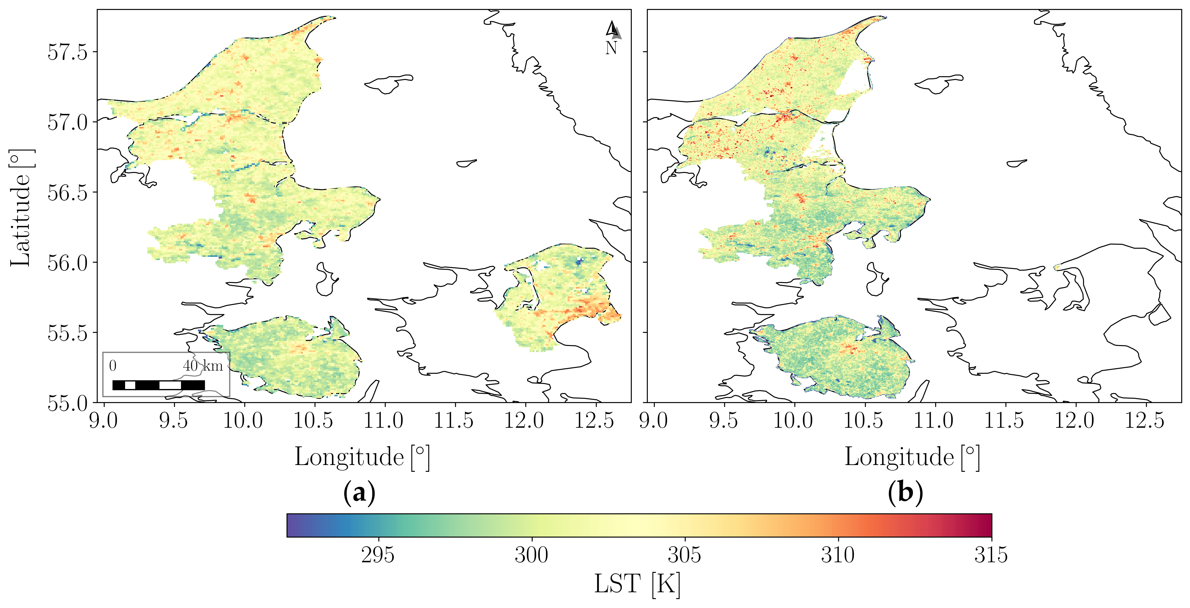
Figure 2. Timeline with the sensing dates of the retrieved Sentinel-3 (blue) and Landsat 8/9 (orange) data as well as a “violin” kernel density plot associated with the former.
Remotesensing 18 02263 g002
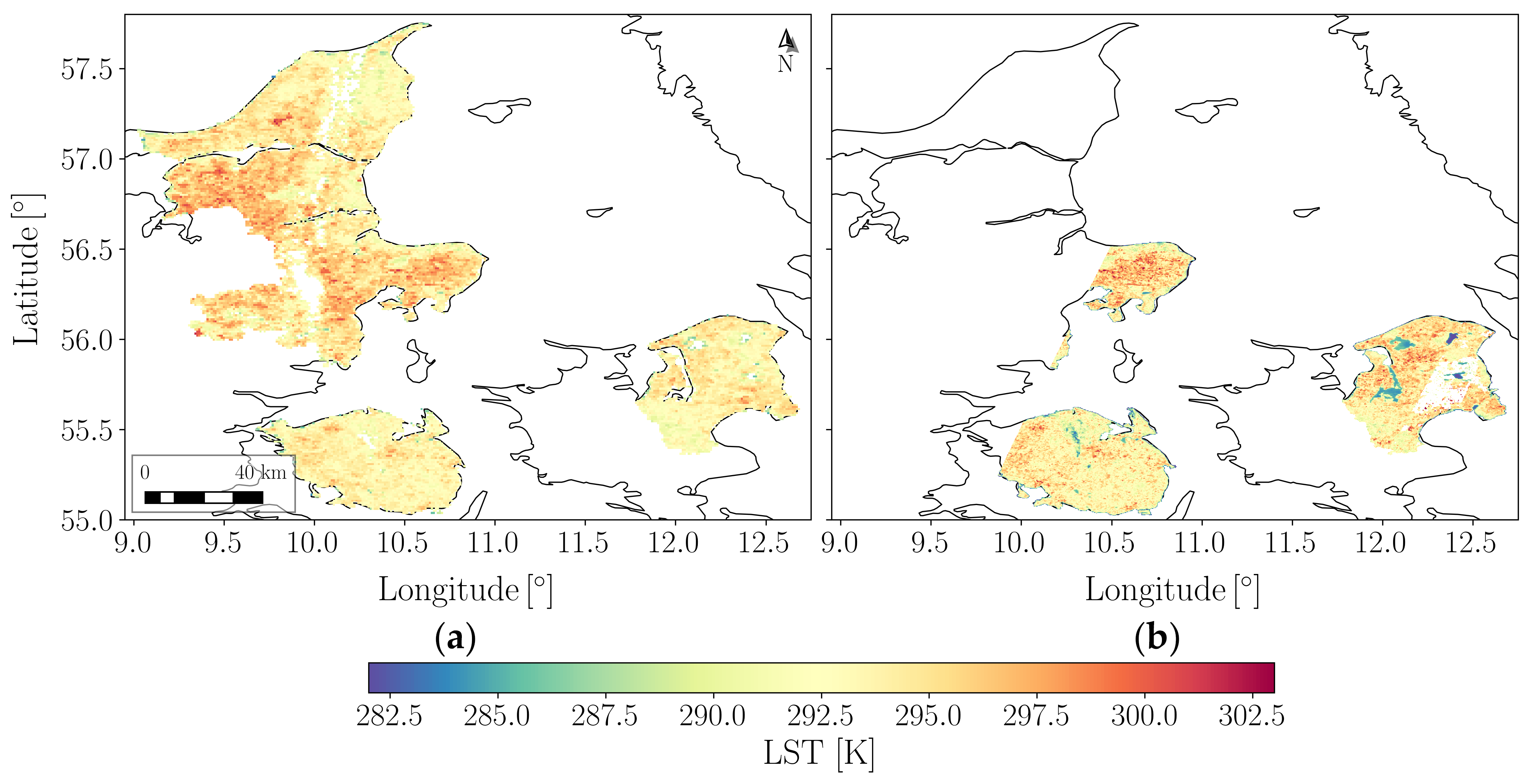
Figure 3. Data architecture considered in the present work (herein “TS” stands for “TimeStamp”; “coarse” and “fine” denote Sentinel-3’s coarse (SLSTR) and fine (SYN) grids; “very fine” denotes Landsat’s original grid).
Remotesensing 18 02263 g003
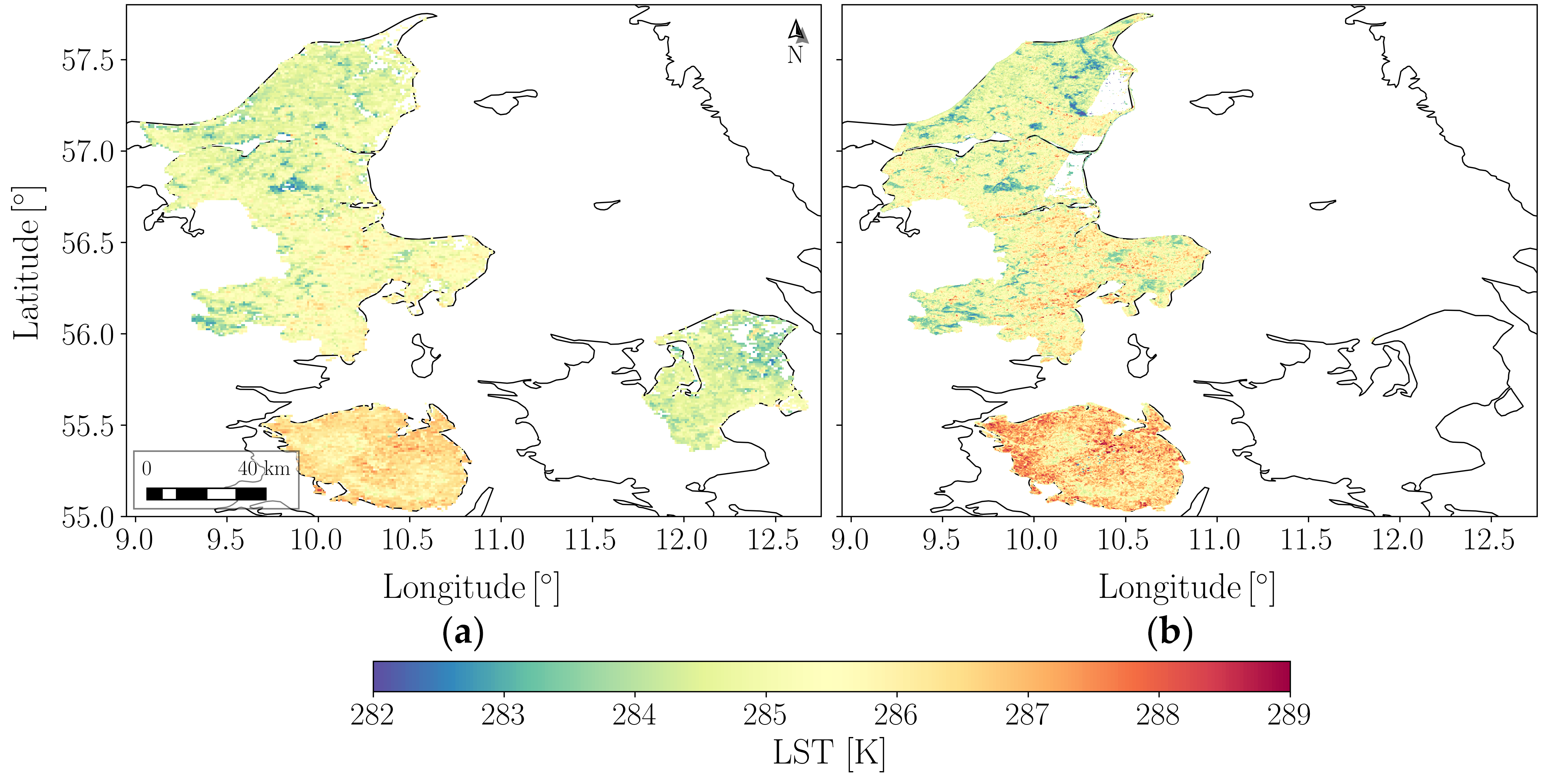
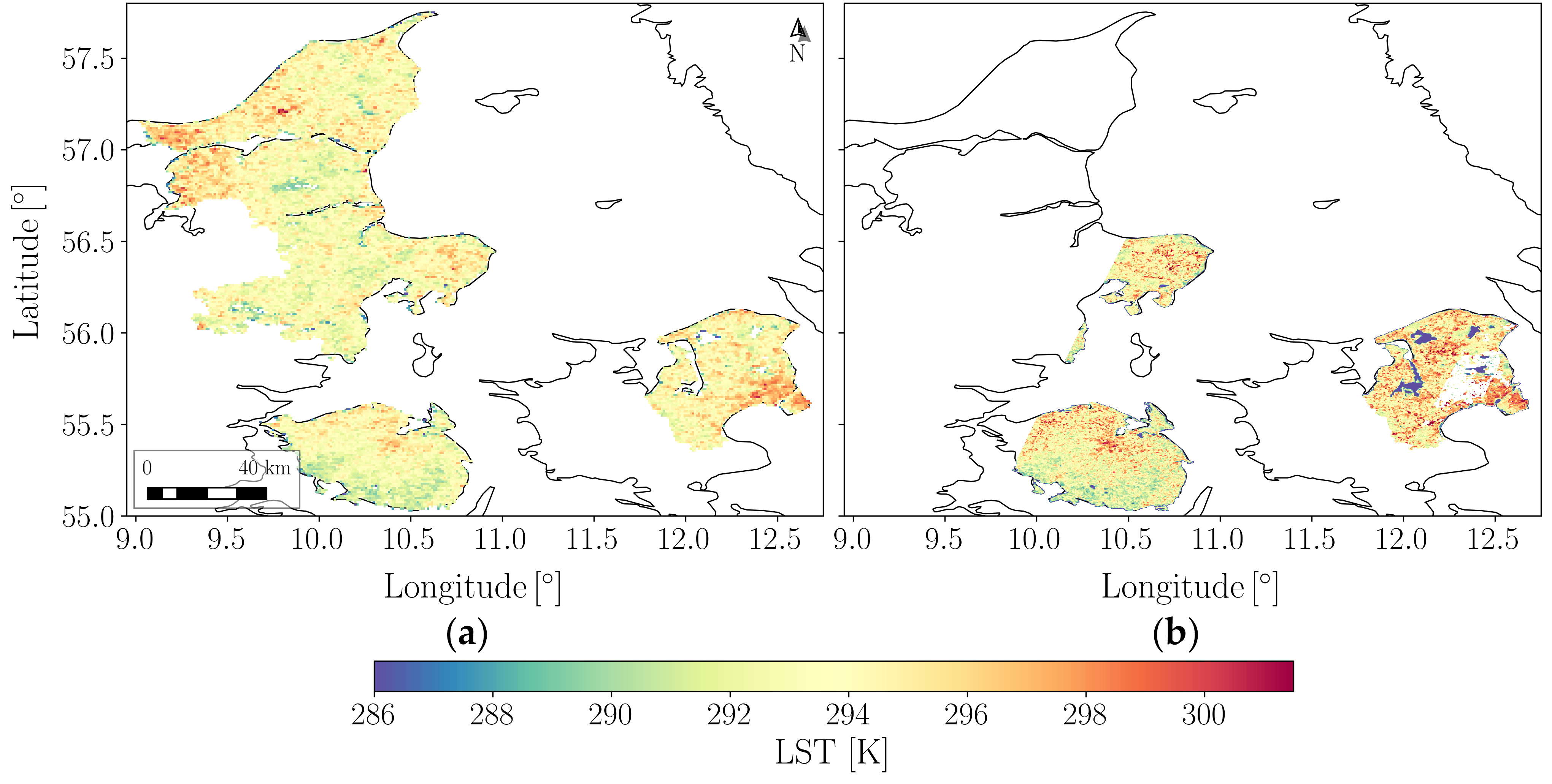
Figure 4. Architecture of the single-timestamp downscaling model, with reference to the equations of the involved residual handling processes.
Remotesensing 18 02263 g004
Figure 5. Architecture of the multi-timestamp downscaling model, considering timestamp-specific standardisation of the spatio-temporal variables ( X x t , LST ). Equations associated with standardisation, de-standardisation and residual handling processes are also herein referred to.
Remotesensing 18 02263 g005
Figure 6. Area of interest of the present work (FUAs of Aalborg, Aarhus, Odense and Copenhagen) and its Local Climate Zones (LCZs) in the common geospatial predictor grid (of resolution 0.002 ).
Remotesensing 18 02263 g006
Figure 7. Percentage frequency distribution of Local Climate Zones in the area of interest.
Remotesensing 18 02263 g007
Figure 8. Pearson correlation matrices (and respective statistical significances) of the numerical coarse data for the test timestamps: as a mean of the correlation matrices for each timestamp (top, (a)), as the correlation matrix of the combined data considering timestamp-specific standardisation of the spatio-temporal variables (centre, (b)) and not considering (bottom, (c)). Coarse Landsat data had been obtained from original data by reprojecting the latter onto Sentinel-3’s coarse grid.
Remotesensing 18 02263 g008
Figure 9. Predicted (straight lines) and actual (stains) coarse Sentinel-3’s LST without timestamp-specific transformation (left-hand side, (a)), with centring (centre, (b)) and with standardisation (right-hand side, (c)) for test timestamps. Prediction is done using a multi-timestamp LR model with FVC as predictor. The stains comprise the 99.9% most probable actual data for each timestamp, and the interiors of the loops comprise the 75% most probable. A counterpart scatter plot is presented in Figure A1 of Appendix A.3.
Remotesensing 18 02263 g009
Figure 10. Predicted versus actual fine Sentinel-3’s LST without residual correction (top row—(ac)) and with it (bottom row—(df)) for test timestamps. Moreover, for these two cases, no timestamp-specific transformation (left-hand side column—(a,d)), centring (centre column—(b,e)) and standardisation (right-hand side column—(c,f)) was considered. Prediction is done using a multi-timestamp LR model with FVC as predictor.
Remotesensing 18 02263 g010
Figure 11. Cross-validation RMSE δ ( RMSE associated with the predicted standardised coarse target) for each number of numerical predictors as a distribution (a) and as the best value (b), obtained with a multi-timestamp LR model considering timestamp-specific standardisation of the spatio-temporal variables.
Remotesensing 18 02263 g011
Figure 12. Cross-validation RMSE δ ( RMSE associated with the predicted standardised coarse target) for each season-dependent Wilkinson formula obtained with a multi-timestamp LR model.
Remotesensing 18 02263 g012
Figure 13. RMSE of all tuned downscaling models obtained in training and testing. Note that Landsat’s coarse and fine data correspond to the original data reprojected to Sentinel-3’s coarse and fine grid, respectively.
Remotesensing 18 02263 g013
Figure 14. RMSE δ ( RMSE associated with the standardised predicted target using the statistics of the respective true target in the standardisation) of all tuned downscaling models obtained in training, cross-validation and testing. Note that Landsat’s coarse and fine data correspond to the original data reprojected to Sentinel-3’s coarse and fine grid, respectively. Also note that there is no cross-validation RMSE δ value for the single-timestamp LR model since this model can only infer for the same timestamp it is trained with, and cross-validation considers different timestamps for training and inference.
Remotesensing 18 02263 g014
Figure 15. Mean Bias Error (MBE) of all tuned downscaling models obtained in training and testing. Note that Landsat’s coarse and fine data correspond to the original data reprojected to Sentinel-3’s coarse and fine grid, respectively.
Remotesensing 18 02263 g015
Figure 16. Mean Absolute Error (MAE) of all tuned downscaling models obtained in training, cross-validation and testing. Note that Landsat’s coarse and fine data correspond to the original data reprojected to Sentinel-3’s coarse and fine grid, respectively.
Remotesensing 18 02263 g016
Figure 17. Probability Density Function (PDF) of the actual and predicted fine LSTs without residual correction for all test timestamps: 30 May 2020 (a), 15 June 2020 (b), 19 April 2022 (c), 19 October 2022 (d), 8 May 2023 (e), 8 June 2023 (f) and 4 September 2023 (g). Note how, for the case of the DMR model, the PDF corresponds to a Dirac delta function centred on the mean of Sentinel-3’s coarse LST for each timestamp.
Remotesensing 18 02263 g017
Figure 18. Probability Density Function (PDF) of the actual and predicted fine LSTs with residual correction for all test timestamps: 30 May 2020 (a), 15 June 2020 (b), 19 April 2022 (c), 19 October 2022 (d), 8 May 2023 (e), 8 June 2023 (f) and 4 September 2023 (g).
Remotesensing 18 02263 g018
Figure 19. Boxplot distributions of the test fine prediction error (with residual correction) of each model for low-, intermediate- and high-value interquantiles of the true fine LST . For both (a) and (b) plots, the whiskers are constrained to the 2 nd and 98 th percentiles of the error distributions. The outliers were removed from the plot (a) and kept in the plot (b).
Remotesensing 18 02263 g019
Figure 20. Predicted versus actual fine LSTs (with residual correction) using the single-timestamp LR model for each test timestamp: 30 May 2020 (a), 15 June 2020 (b), 19 April 2022 (c), 19 October 2022 (d), 8 May 2023 (e), 8 June 2023 (f) and 4 September 2023 (g). The stains comprise the 99.9% most probable actual data for each LCZ, and the interiors of the loops comprise the 75% most probable. A counterpart scatter plot is presented in Figure A2 of Appendix A.3.
Remotesensing 18 02263 g020
Figure 21. Predicted versus actual fine LSTs (with residual correction) using the multi-timestamp NN model for each test timestamp: 30 May 2020 (a), 15 June 2020 (b), 19 April 2022 (c), 19 October 2022 (d), 8 May 2023 (e), 8 June 2023 (f) and 4 September 2023 (g). The stains comprise the 99.9% most probable actual data for each LCZ, and the interiors of the loops comprise the 75% most probable. A counterpart scatter plot is presented in Figure A3 of Appendix A.3.
Remotesensing 18 02263 g021
Figure 22. Boxplot distributions of the test fine prediction error (with residual correction) of each model for each LCZ class, with the outliers removed. The whiskers are constrained to the 2 nd and 98 th percentiles of the error distributions.
Remotesensing 18 02263 g022
Figure 23. Boxplot distributions of the test fine prediction error (with residual correction) of each model for each LCZ class, with outliers. The whiskers are constrained to the 2 nd and 98 th percentiles of the error distributions.
Remotesensing 18 02263 g023
Figure 24. Boxplot distributions of the estimated fine residuals (that is, the finely interpolated coarse residuals), | ε ^ fine | , for different ranges of the fine prediction errors obtained when considering residual correction. The whiskers are constrained to the 2 nd and 98 th percentiles of the estimated fine residuals.
Remotesensing 18 02263 g024
Figure 25. Boxplot distributions of the differences between Sentinel-3 and Landsat’s true coarse LST for each timestamp and LCZ class. The whiskers are constrained to the 2nd and 98th percentiles of the   LST differences.
Remotesensing 18 02263 g025
Figure 26. Boxplot distributions of the test scores in fine prediction (with residual correction): R 2 (a), Root Mean Squared Error of the standardised predicted LST using the statistics of the true target in the standardisation ( RMSE δ ) (b), Root Mean Squared Error (RMSE) (c), Mean Absolute Error ( MAE ) (d), Mean Absolute Error of the standardised predicted LST using the statistics of the true target in the standardisation ( MA E δ ) (e) and Mean Bias Error ( MBE ) (f). The whiskers are constrained to the 0th and 100 th percentiles of the error distributions.
Remotesensing 18 02263 g026
Figure 27. Sentinel-3 coarse (a) and Landsat fine (b) LST for Odense on 8 June 2023.
Remotesensing 18 02263 g027
Figure 28. Predicted fine LST (with residual correction) for Odense on 8 June 2023: multi-timestamp Dummy Mean Regression (a), multi-timestamp Linear Regression (b), multi-timestamp Neural Net (c), multi-timestamp Random Forest (d), multi-timestamp Gradient Boosting (e) and single-timestamp Linear Regression (f).
Remotesensing 18 02263 g028
Figure 29. Fine prediction error (with residual correction) obtained by the downscaling models for Odense on 8 June 2023: multi-timestamp Dummy Mean Regression (a), multi-timestamp Linear Regression (b), multi-timestamp Neural Net (c), multi-timestamp Random Forest (d), multi-timestamp Gradient Boosting (e) and single-timestamp Linear Regression (f).
Remotesensing 18 02263 g029
Figure 30. Importance of each feature in the multi-timestamp GB model. Feature importance is herein defined using XGBoost package as the average information gain across all tree splits the feature is used in.
Remotesensing 18 02263 g030
Table 1. Matching dates between Sentinel-3 and Landsat 8/9 and corresponding time difference.
Sentinel TimestampLandsat TimestampLandsat
Path/Row
Time Difference in Minutes
30 May 2020 10:1730 May 2020 10:19L8 196/20-212.15
15 June 2020 10:0215 June 2020 10:19L8 196/20-2117.3
19 April 2022 10:1519 April 2022 10:13L9 195/21-221.81
19 October 2022 10:1019 October 2022 10:20L9 196/20-2110.59
8 May 2023 9:598 May 2023 10:13L9 195/21-2214.77
8 June 2023 9:558 June 2023 10:19L8 196/20-2124.49
4 September 2023 10:134 September 2023 10:20L9 196/20-216.46
Table 3. Cross-validation RMSE δ ( RMSE associated with the predicted standardised coarse target) of best combinations of numerical predictors for each number of predictors, from worst to best.
Numerical PredictorsNumber of Numerical Predictors RMSE δ
FVC 1 0.926
FVC ,   IMD 2 0.895
FVC ,   IMD ,   NDWI 3 0.845
FVC ,   IMD ,   NDWI ,   TCD 4 0.832
FVC ,   IMD ,   NDWI ,   TCD ,   DCOAST 5 0.820
FVC ,   IMD ,   NDWI ,   TCD ,   DCOAST ,   DEM 6 0.820
FVC ,   IMD ,   NDWI ,   TCD ,   DCOAST ,   DEM ,   TOPEX 7 0.819
FVC ,   IMD ,   NDWI ,   TCD ,   DCOAST ,   DEM ,   TOPEX ,   UD 8 0.819
FVC ,   IMD ,   NDWI ,   TCD ,   DCOAST ,   DEM ,   TOPEX ,   UD ,   NDVI 9 0.819
Table 4. Tuned hyperparameter values for the models based on Neural Net, Random Forest, and Gradient Boosting within multi-timestamp architectures.
ModelHyperparameterTuned Value
Neural Network (NN)Numerical scalingStandardisation
Hidden layersThree hidden layers (21, 23 and 32 units)
Initial learning rate1.14 × 10−3
L2 regularisation term (α)1.15 × 10⁻⁴
Random Forest (RF)Numerical scalingStandardisation
Categorical encodingDummy encoding (Season)
Number of trees1225
Maximum tree depth14
Minimum loss reduction for split (γ)2.47
Fraction of data records for each split (“subsample”)0.72
Fraction of features for each split (“colsample_bytree”)0.97
Gradient Boosting (GB)Numerical scalingStandardisation
Categorical encodingDummy encoding (Season)
Number of trees1185
Maximum tree depth14
Minimum loss reduction for split (γ)0.30
Fraction of data records for each split (“subsample”)0.79
Fraction of features for each split (“colsample_bytree”)0.97
Learning rate0.019
L1 regularisation term (α)0
L2 regularisation term (λ)0.098
Disclaimer/Publisher’s Note: The statements, opinions and data contained in all publications are solely those of the individual author(s) and contributor(s) and not of MDPI and/or the editor(s). MDPI and/or the editor(s) disclaim responsibility for any injury to people or property resulting from any ideas, methods, instructions or products referred to in the content.