Scale Effects on Dominant Drivers of Commercial Plantation Productivity: Novel Insights from High-Resolution Multi-Sensor UAV Remote Sensing and Interpretable AI

Highlights

What are the main findings?

• Vegetation vigor is controlled by different drivers across spatial scales.
• Canopy structure, soil–canopy interactions, and terrain factors dominate at fine, intermediate, and broad scales, respectively.

What is the implication of the main finding?

• Precision forestry should apply scale-matched management strategies.
• UAV remote sensing and interpretable AI can support site-specific plantation management.

Abstract

Subtropical mountain economic tree plantations are constrained by pronounced spatial heterogeneity in resource availability, yet the spatial scales at which soil properties, topography, and canopy structure regulate vegetation vigor remain poorly resolved. To address this gap, a spatially consistent multi-scale dataset combining 10 m high-density soil sampling, UAV-LiDAR, and multispectral remote sensing was used to quantify the scale-dependent drivers of the Leaf Chlorophyll Index (LCI) across 3–50 m within a Chinese hickory (Carya cathayensis Sarg.) plantation. The relative contributions of canopy, soil, and topography to LCI were decomposed across scales using an interpretable machine-learning framework (XGBoost–SHAP). At fine scales (3–10 m), vegetation vigor was primarily controlled by tree-level canopy structure, particularly tree height, reflecting localized resource acquisition. At intermediate scales (10–20 m), a distinct coupling window emerged, characterized by increased interaction complexity: LCI was predominantly driven by interactions between canopy structure and soil nutrient availability, whereas single-factor effects weakened. Notably, at 20 m this interaction pattern largely weakened and reverted to single-metric dominance. At broader scales (>30 m), complex interactions re-emerged, and dominant SHAP contributions shifted from nutrients and canopy structure toward topography and soil texture. These findings reconcile strong fine-scale drivers with weaker predictability at intermediate extents and demonstrate that soil–canopy relationships reorganize across spatial scales rather than remaining static. On the basis of these findings, a scale-hierarchical framework for precision forestry is proposed that aligns management interventions with the ecological scales at which dominant correlates operate across spatial supports.

1. Introduction

Subtropical mountain economic tree plantations constitute a critical component of regional agricultural economies and ecosystem service provision [1,2,3,4]. However, the productivity and vegetative vigor of these systems are strongly constrained by the inherent heterogeneity of mountainous landscapes [4,5,6]. Complex terrain induces significant spatial heterogeneity in hydrothermal conditions, soil formation processes, and nutrient distributions [6,7,8,9]. Consequently, management interventions, including fertilization, pruning, and density regulation, can be effective at the tree or plot scale but often yield inconsistent outcomes when applied uniformly across heterogeneous terrain [10,11,12]. A fundamental challenge is therefore to explicitly characterize and explain the spatial variation in vegetation growth within mountain plantations. Vegetation vigor in these systems is governed by coupled controls of soil properties, topography, and canopy structure rather than by any single factor.

The multidimensional controls on forest growth are well-established [13,14]. Edaphic properties, such as pH, EC, and nutrient content, regulate the root-zone resource availability and uptake [15]. Topographic factors like slope and curvature regulate growth through the redistribution of water and solar radiation [16,17]. Meanwhile, canopy structure, characterized by height, coverage, and complexity, modulates the light interception and evapotranspiration dynamics, thereby creating a competitive landscape that feeds back into vegetation physiology [18,19]. Importantly, these controls are interdependent: topography and soils jointly shape canopy development, while canopy structure in turn alters how soil and hydrological resources translate into growth through interception and transpiration processes [20,21]. Despite these factors being widely reported, their influence on vegetation in mountainous environments often exhibits strong scale dependence [22,23,24].

Ecological processes operate across characteristic spatial domains, ranging from meter-scale rhizosphere processes to decameter-scale neighborhood competition and broader hillslope hydrothermal gradients [25,26,27]. When environmental variables are aggregated at different spatial supports, their statistical relationships with vegetation responses can shift substantially—a phenomenon known as the “scale of effect” [28,29,30,31]. Conceptually, the scale of effect refers to the spatial support at which the statistical association between a predictor and the response variable is strongest; operationally, throughout this study it denotes the buffer radius used to aggregate each predictor when modeling the Leaf Chlorophyll Index [31,32]. However, uncovering these scale-dependent relationships is fundamentally constrained by “scale mismatches” in current research. Studies often rely on incompatible data supports, such as coupling point-based soil data with coarse-resolution remote sensing, which fails to systematically identify the optimal scales of diverse ecological drivers [28,33,34]. The scarcity of paired, scale-consistent, and high-precision datasets has further limited robust multi-scale inference in economically significant forests.

Emerging ultra-high-resolution remote sensing bridges critical observational gaps in mountain ecosystems. Unmanned aerial vehicles (UAVs) provide the spatial resolution necessary to capture fine-scale growth fragmentation [35,36,37]. The UAV-derived Leaf Chlorophyll Index (LCI) serves as a robust proxy for physiological vigor [32,38,39], distinguished by its high sensitivity to foliar variations and reduced saturation effects [40,41,42,43]. Complementarily, Light Detection and Ranging (LiDAR) resolves vertical structural metrics that spectral indices cannot [44,45]. LiDAR quantifies complex 3D attributes—such as canopy height and stratification—which are pivotal for understanding light interception and biomass accumulation [46,47,48].

These observational advances motivate a sharper scientific question: do the dominant drivers of canopy vigor and their interactions occupy distinct characteristic scales, and if so, how do they reorganize as the spatial support is enlarged? Recent work has begun to address this question in adjacent settings. Milodowski [49] reported pronounced scale variance in carbon dynamics across fragmented mixed-use landscapes, and Bañares-de-Dios [50] demonstrated scale-dependent reorganisation of community assembly in tropical montane forests. However, a study that resolves the characteristic scales of multiple coupled drivers under scale-consistent high-density sampling within a subtropical economic forest remains absent. The present study addresses this gap by leveraging a paired structural–physiological dataset (UAV-LCI and LiDAR) collected at high density.

With this dataset, the aim is to disentangle the multi-scale drivers of vegetation performance. Building on scale theory, the study hypothesizes that the dominant drivers of vegetation response reorganize systematically across spatial supports: fine scales are expected to emphasize local soil resource supply and canopy neighborhood interactions, whereas broader scales should increasingly reflect terrain-mediated hydrothermal constraints. Specifically, this study tested (i) whether the scale of effect differs significantly among soil, canopy, and terrain variables, and (ii) how their relative importance and interactive structures shift with increasing spatial support.

To explicitly address the aforementioned “scale mismatches” and the pervasive reliance on incompatible, low-precision data supports, this study combines a spatially consistent multi-scale sampling design with interpretable machine learning. The study focused on a Chinese hickory (Carya cathayensis Sarg.) plantation, a representative subtropical economic forest, and leverages high-density soil sampling at a 10-m resolution. This dataset provided the necessary statistical foundation to aggregate soil properties across neighborhood scales ranging from 3 to 50 m without interpolation bias. Integrating these data on a unified scale creates a rare opportunity to rigorously identify scale effects. Nevertheless, relationships among these multi-source variables are often non-linear and subject to complex interactions that traditional linear models cannot adequately capture [51].

To address these complexities, this study applied Machine learning (ML) algorithms, which are well-suited for modeling the non-linearities, thresholds, and high-order relationships inherent in mountain ecosystems [52,53,54]. To overcome the “black box” nature of ML, this study employed Shapley Additive exPlanations (SHAP). This framework enables quantification of variable contributions and directionality [55] and critically facilitates the use of interaction SHAP values to reveal how the interplay between factors evolves across spatial scales [56]. Building on this approach, this study developed a multi-scale integrated and interpretable modeling framework to identify the dominant factors and characteristic scales governing the vegetation status of mountain economic tree plantations.

Specifically, this study aims to: (i) quantify the scale-specific contributions of environmental drivers to canopy physiological vigor (LCI) across 3–50 m neighborhoods, identifying both the global optimal scale and variable-specific characteristic scales, and (ii) characterize the interaction networks among key variables and their scale dependence, thereby decoding the multidimensional coupling mechanisms and non-linear ecological synergies underlying vegetation performance. Soil nutrient drivers are hypothesized to exhibit a localized peak effect at fine scales, expected within 8–10 m (the effective integration scale of root extension and soil microsite nutrient cycling), and that canopy structural drivers peak slightly finer, within 5–10 m, on the order of individual crown projection diameter, whereas broader-scale variation is predominantly governed by topographic constraints. By integrating high-precision empirical sampling with interpretable cross-scale modeling, this work establishes a robust mechanistic foundation and an actionable analytical framework for the precision management of heterogeneous mountain plantations.

2. Materials and Methods

2.1. Study Area

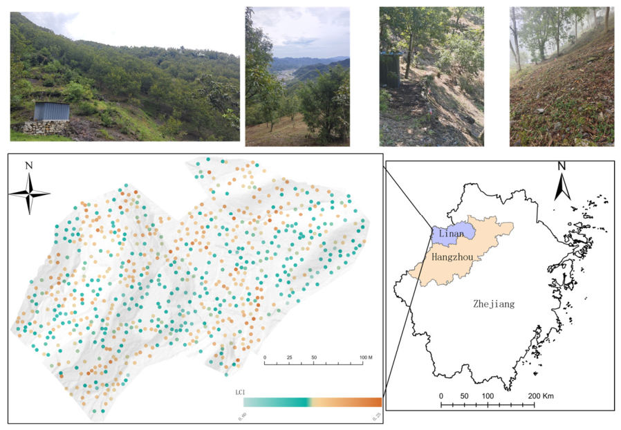
The study site is located in Daoshi Town, Lin’an District, Hangzhou City, Zhejiang Province, China, which is a core production area of Chinese hickory (Carya cathayensis Sarg.) in a subtropical mountainous economic-forest landscape. To minimize potential effects of residential activities and edge conditions, this study selected a contiguous Chinese hickory plantation that is distant from residential areas. The plot measures approximately 380 m × 220 m (about 8.36 ha), with an elevation range of 510–590 m and slopes ranging from 0.7° to 66°. The plot includes both sun-facing and shaded aspects and covers multiple terrain positions, including hillslopes, relatively flat areas, and valley sections. Soil sampling reference points were arranged in a checkerboard pattern with 10 m spacing. At each reference point, a mixed soil sample was collected beneath the canopy projection of the nearest tree within a 5 m radius. All sampling locations were georeferenced using a real-time kinematic (RTK) system (Huace X11, Shanghai Huace Navigation Technology Ltd., Shanghai, China), with a positioning error of less than 1 cm, to ensure accurate spatial alignment for subsequent analyses. A total of 808 mixed soil samples were collected in this study. This corresponds to the number of tree apex points (n = 808).

2.2. Data Collection

2.2.1. Soil Sampling and Analysis

At each sampling site, soil cores were collected using a handheld soil core with a 5.5 cm diameter at a depth of 0–20 cm. This depth was chosen because it represents the biologically active surface horizon most relevant to plant uptake and microbially mediated nutrient cycling and is widely used in regional soil inventories for comparability across ecosystems.

Soil samples were transported to the laboratory in portable coolers at 4 °C. Air-dried soil subsamples were passed through a 2-mm mesh for physical and chemical analyses. Soil pH was measured using a pH meter (Seven compact pH, Mettler Toledo, Zurich, Switzerland). Soil electrical conductivity (EC) was determined using a conductivity meter (SevenCompact, Mettler Toledo, Zurich, Switzerland). NH₄⁺−N, NO₃⁻−N, NO₂⁻−N and Available Phosphorus (AP) were quantified using a discrete chemistry analyzer following extraction (Smartchem 450, KPM Analytics (Beijing), Beijing, China). Additionally, Available Potassium (AK) content was determined by ICP-OES after extraction. Soil texture fractions (clay, silt, sand) were determined using a laser particle size analyzer (Malvern Mastersizer 3000, Malvern Panalytical Ltd., Malvern, UK).

2.2.2. Derivation of LCI, Topographic Variables, and Canopy Structure

Canopy activity was characterized using the Leaf Chlorophyll Index (LCI), derived from multispectral imagery acquired by a DJI Mavic 3M (DJI-Innovations, Shenzhen, China) at a flight altitude of approximately 40 m relative to the canopy. Image processing and orthomosaic generation were performed in DJI Terra (v4.1.0). LCI was calculated as:

$$LCI = (NIR - RedEdge) / (NIR + Red)$$

where NIR, RedEdge, and Red denote reflectance in the near-infrared, red-edge, and red bands, respectively.

Topographic and structural data were derived from airborne LiDAR collected via a DJI L1 sensor mounted on a DJI M300 RTK platform (40 m AGL). Point cloud processing yielded both a Digital Elevation Model (DEM) and a Digital Surface Model (DSM). Terrain (DEM-based) and surface (DSM-based) derivatives, including slope and curvature, were calculated in ArcGIS Pro (3.6.0) using a 3 × 3 window size. Solar radiation (direct and diffuse) was modeled for the growing season (April–November) using the Spatial Analyst tools.

Individual tree detection (ITD) and height extraction were conducted in ArcGIS Pro (3.6.0) based on the Canopy Height Model (CHM), defined as the difference between the DSM and the DEM. A local maximum algorithm was applied using a 5 × 5 circular moving window to identify candidate tree apices. To filter understory vegetation and noise, a height threshold of 2 m was applied. The remaining local maxima were vectorized to point features representing tree apices, with tree heights assigned from the corresponding CHM values. Finally, these locations were validated and corrected through visual inspection of the RGB orthomosaics. A total of 808 individual trees passed the height threshold and visual validation and were retained as the analysis units for all subsequent modeling.

For multi-scale analysis, predictor variables were aggregated within circular buffers centered on each tree-apex point at radii of 3, 5, 8, 10, 12, 15, 20, 30, and 50 m. The aggregation statistic was the median, selected for its robustness to extreme canopy values and to outliers among the input pixels. Where a buffer extended beyond the plot boundary, no extrapolation, imputation, or padding was applied; the aggregation used only the in-plot pixels available within the buffer. The response variable (LCI) was extracted at the 808 tree-apex points and was not aggregated across scales.

All geospatial datasets were projected to the CGCS2000 (3 Degree GK CM 120E) coordinate system with a spatial resolution of 0.05 m. To ensure data consistency, all raster layers were spatially co-registered in ArcGIS Pro (3.6.0) to achieve strict pixel-to-pixel alignment prior to analysis.

2.3. Machine Learning Process

The modeling operates on a scale-consistent dataset in which the multi-scale neighborhood-aggregated canopy, soil, terrain, and radiation variables serve as predictors (model inputs) and tree-level Leaf Chlorophyll Index serves as the response (model output). XGBoost was chosen because gradient-boosted trees efficiently capture the non-linearities and threshold-like responses typical of mountain ecosystems; native L1/L2 regularization curbs overfitting at moderate sample sizes; and native compatibility with TreeExplainer-based SHAP and exact k-SII interaction computation makes attribution directly comparable across the nine scales [57].

Model training and interpretability analyses were executed in a Python 3.12.0 environment. The XGBoost model was implemented using the scikit-learn API. For the study site dataset, the feature space was configured by extracting columns based on indices relevant to the analysis. The data were subsequently partitioned into training (70%) and validation (30%) sets using a fixed random seed of 42. The random partition was retained for three reasons. (i) Random splitting inflates R² only when the response variable or model residuals exhibit appreciable spatial autocorrelation [58,59,60]; in this study, the global Moran’s I of LCI is 0.267 (Table S1), substantially below all soil chemical, textural, and elevation predictors (Moran’s I = 0.86–0.97). (ii) When the response autocorrelation is low and sampling covers the entire prediction domain, random cross-validation gives near-unbiased accuracy estimates, whereas spatial block CV introduces pessimistic bias [61,62,63,64,65]. (iii) The global Moran’s I of model residuals at three representative scales (Table S2) is non-significant at 15 m (0.049, p = 0.227) and 50 m (0.073, p = 0.079), and although it remains modest at 3 m (0.181, p < 0.001), it is one-third smaller than that of LCI itself, providing empirical confirmation that prediction has not been driven by spatial proximity.

To further verify that the random-split accuracy estimates were not inflated by residual spatial autocorrelation, an additional spatial cross-validation was performed as a sensitivity analysis. In contrast to the random partition, the 808 trees were divided according to their geographic coordinates: a spatially contiguous block comprising 160 trees (≈20% of the dataset) was withheld as a spatially separated validation set, and the remaining 648 trees were retained for training (Figure S6). Because the training and validation samples occupy distinct, non-interleaved portions of the plot, short-range autocorrelation across the two sets is minimized, so that any accuracy inflation arising from spatial proximity between training and test points would manifest as a decline in validation performance. The XGBoost model was re-fitted on the spatially blocked training set following the same hyperparameter-optimization protocol described above, and its accuracy on the held-out block was quantified by the coefficient of determination (R²).

Hyperparameter optimization was conducted via Bayesian optimization (BayesSearchCV in scikit-optimize) with 5-fold cross-validation. To ensure robust convergence, the search was configured for a maximum of 3000 evaluations. The hyperparameter search space was defined as follows: n_estimators (50–1000), max_depth (3–12), learning_rate (0.01–0.3), subsample and colsample_bytree (0.6–1.0), reg_alpha (0–2.0), reg_lambda (0.5–3.0), min_child_weight (1–10), and gamma (0–0.5). The tree_method was fixed to ‘hist’ to accelerate computation. Parallel resources were managed with unified logging to ensure stability and traceability throughout the process.

Model interpretability was assessed using the SHAP and SHAP-IQ packages. Global feature importance was quantified by calculating SHAP values using the entire dataset. High-order feature interactions were analyzed based on the k-SII index (SHAPIQ_INDEX = ‘k-SII’) to capture both pairwise and three-way effects (SHAPIQ_MAX_ORDER = 2, 3). The interaction analysis prioritized the TreeExplainer approach, defaulting to a simplified strategy if necessary. To balance computational efficiency with accuracy, the computation budget was set to 2048 with a maximum of 300 compute samples, and visualizations were generated based on a subset of 500 samples. To guarantee reproducibility, the random seed was fixed at 42 during the interpretation phase, with strict constraints applied to CPU usage, maximum parallel processes, and memory thresholds to prevent resource exhaustion. All complementary statistical analyses and data visualizations were performed in Python 3.12.0 and R 4.5.2.

3. Results

3.1. Spatial Patterns of Vegetation Vigor and Multidimensional Driving Factors

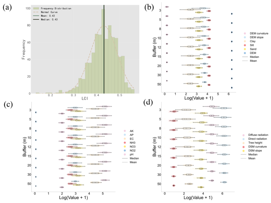
The LCI exhibited a stable distribution without the saturation or right-skewness effects often observed in dense, heterogeneous forests (Figure 1 and Figure 2a). Specifically, LCI values showed a unimodal, approximately normal distribution (Mean = 0.43, Median = 0.43), spanning a broad range from approximately 0.2 to 0.6. Regarding the driving factors, their mean values changed little across neighborhood scales, whereas their spatial variability declined steadily as neighborhood size increased, as reflected by a decreasing coefficient of variation (CV) (Figure 2b–d). For instance, the CV of TH decreased substantially from 58.19% at the 3-m scale to 22.05% at the 50-m scale. In contrast, other variables exhibited more modest reductions, such as EC, where the CV declined from 29.99% at the 3-m scale to 24.47% at the 50-m scale, indicating comparatively persistent heterogeneity across scales.

Furthermore, the driving factors exhibited substantial spatial heterogeneity across the landscape. Topographic features, including slope and elevation, and canopy structural metrics, such as tree height, displayed distinct ranges of variation (Table S1). Notably, soil chemical properties, particularly available nutrients such as AK, AP and inorganic nitrogen forms, demonstrated exceptionally high spatial heterogeneity (Figures S1–S3), highlighting pronounced microsite variability in resource availability.

3.2. Scale-Dependent Relationships Between LCI and Driving Factors

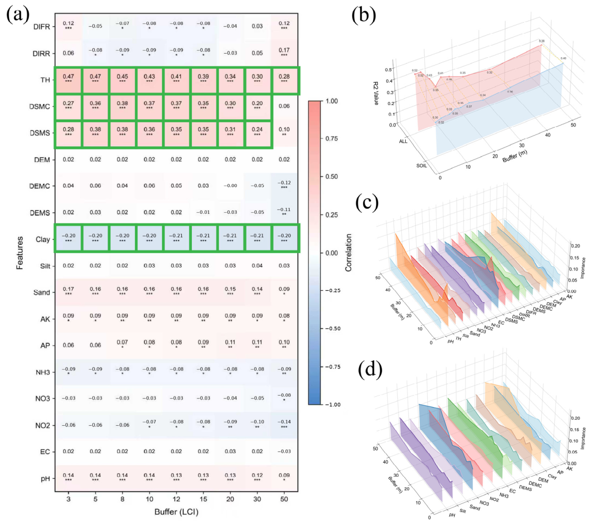
Correlation analysis showed that the strength of association between each individual factor and LCI varied with spatial scale (Figure 3a; Figure S4). This study observed significant positive correlations between LCI and canopy structural metrics, including tree height (TH) and density metrics (DSMC and DSMS). However, their optimal scales diverged remarkably: the correlation strength of TH attenuated continuously with increasing scale, whereas the explanatory power of DSMC and DSMS exhibited a distinct “peak effect”, maximizing at the 5-m and 8-m scales before subsequently dissipating as the neighborhood expanded.

In contrast, among soil properties, clay content (Clay) maintained a stable and significant negative correlation across all evaluated scales. Although other soil metrics also demonstrated statistically significant associations with LCI at specific spatial supports, these baseline correlations were generally weak, suggesting that linear bivariate relationships alone are insufficient to capture the complexity of vegetation–environment coupling.

To systematically evaluate these dynamics and address the overwhelming influence of canopy structure, this study established a comparative modeling framework. First, the performance of the full XGBoost model—encompassing all canopy, soil, and topographic drivers—exhibited a pronounced, non-monotonic scale effect (Figure 3b). This full model achieved its highest explanatory power at the ultra-fine 3 m scale (R² = 0.52). Following an initial decline, its performance displayed a secondary peak at the 5-m scale (R² = 0.41), then decreased gradually before experiencing a final resurgence at the 50-m scale (R² = 0.38). Meanwhile, the spatial cross-validation indicated that this fine-scale performance was largely retained under spatially separated validation (R² = 0.488; Figures S6 and S7), suggesting that it reflects genuine structure–function relationships rather than spatial proximity between samples. Crucially, because canopy structural metrics inherently dominate the LCI signal and may obscure underlying site conditions, this study subsequently constructed an “abiotic-only” model that isolated topography and soil properties. Strikingly, in stark contrast to the fluctuating trajectory of the full model, the explanatory power of this isolated abiotic model exhibited a robust, monotonically increasing trend as the spatial scale expanded, indicating that terrain and soil constraints become progressively more detectable as fine-scale structural variability is spatially averaged.

Beyond overall model performance, feature importance analysis captured the complex non-linear relationships and revealed a dramatic spatial reorganization of driver dominance across scales (Figure 3c,d and Figure S5). In the full model, canopy structure (primarily TH) generally ranked as the paramount driver, followed closely by soil electrical conductivity (EC) and Clay, while soil available nitrogen content also exerted considerable influence at specific scales. More importantly, the relative importance of individual drivers exposed a critical ecological transition window. TH dominated at fine scales (XGBoost native feature importance = 0.190 at 3 m and 0.163 at 5 m, both ranked 1st among 18 predictors; Figure 3c, Table S4), but its importance dropped sharply after 5 m, to 0.062 at 12 m (rank 3) and reached a transient minimum of 0.043 at 15 m (rank 10)—a cumulative reduction of 77.4% from the 3 m peak and a drop of seven rank positions between 12 m and 15 m—before recovering to 0.089 at 30 m and 0.149 at 50 m (rank 1 at both). Within this 10–15 m window, horizontal canopy density (DSMS) surpassed TH to become the leading driver (importance = 0.159 at 15 m), accompanied by an increase in the importance of soil EC. As the spatial scale extended beyond 20 m, the influence of both DSMS and EC gradually diminished. Furthermore, the dynamic trajectory of Clay closely mirrored the bimodal trend of TH, ultimately securing its position as the second most important factor at the 30-m scale. Additionally, while available potassium (AK) appeared as the second leading factor at the broader 50-m scale, this rank shift reflected the relative decline of other predictors rather than an absolute amplification of AK’s marginal contribution, which remained comparatively stable across scales.

3.3. Scale-Dependent Interaction Networks Among Driving Factors

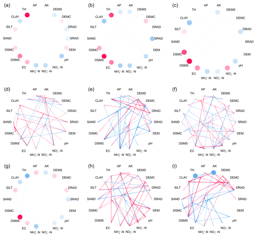
To further disentangle the coupling mechanisms underlying vegetation vigor, this study constructed interaction networks based on SHAP interaction values across multiple spatial scales (Figure 4). The topology and complexity of these networks exhibited distinct scale-dependent evolution patterns.

At the 3–8 m scale, the interaction network was characterized by weak connectivity, primarily dominated by interactions among canopy structural metrics. As the spatial scale expanded to the 10–20 m range, network complexity increased significantly, indicating intensified coupling among the driving factors. However, a precipitous drop in network complexity occurred at the 20-m scale, after which it rebounded to previous levels. Specifically, TH acted as a central hub in the interaction networks at the 3–8 m scale, exhibiting strong links with soil pH, EC, and topography. However, TH lost this centrality within the 10–15 m scale window, where it was superseded by other canopy structural metrics. Notably, the interaction between available nitrogen and canopy structure was most prominent at the 12-m scale, contributing significantly to the model’s explanatory power. Furthermore, the nature of interactions shifted across scales. While intra-canopy structural interactions were prevalent at the 3–8 m scale, soil–canopy structure interactions (e.g., EC–TH) became increasingly pronounced at scales > 10 m, indicating a transition from structure-dominated regulation toward coupled resource–structure modulation.

4. Discussion

Uncovering the true scale-dependent mechanisms governing mountain forest ecosystems has historically been hindered by sparse, plot-based sampling designs [66]. Such traditional approaches inevitably smooth over localized hotspots and obscure critical microsite variability. By deploying an unprecedented 10-m high-density sampling framework coupled with interpretable machine learning, our study provides a continuous, unbiased characterization of spatial heterogeneity across nested scales. The overarching findings demonstrate that the relationships between vegetation vigor and its multi-dimensional drivers in subtropical economic plantations are inherently scale-dependent, rather than spatially invariant [67]. Specifically, as the spatial support expanded from 3 m to 50 m, the spatial variability in most drivers declined markedly despite stable central tendencies (Figure 1). The high-density sampling design strengthens confidence that the observed multi-scale patterns reflect ecological aggregation processes rather than interpolation artifacts (Figure 1).

4.1. Scale Dependence and Shifting Regulatory Mechanisms of Vegetation–Environment Coupling

The observed non-monotonic scale response is interpreted below across three nested ecological domains. This distinct U-shaped trajectory suggests that vegetation vigor is not governed by a single, spatially uniform process. Instead, it reflects the complex superposition of multiple ecological controls acting across distinct spatial domains. This study proposes that the intermediate scales represent a critical zone of “signal dilution”—a transitional domain where fine-scale physiological heterogeneity is partially averaged out, yet broader-scale environmental and topographic gradients have not yet fully emerged as the dominant constraints [49,50].

Beyond changes in individual driver importance, scale dependence was further manifested as a reorganization of interaction structures among drivers. SHAP-based interaction analysis revealed a transition from relatively sparse, canopy-dominated interactions at fine scales (3–8 m) to more densely connected soil–structure interaction networks at intermediate scales (10–20 m), and finally to interaction patterns increasingly constrained by environmental factors at scales exceeding 30 m (Figure 4). It should be noted that SHAP interaction values quantify model attribution and may be partly amplified by predictor collinearity; the interaction patterns reported here should therefore be read as model-based hypotheses about coupling rather than as direct evidence of ecological process. These results indicate that scale dependence reflects not only quantitative shifts in driver strength but also qualitative changes in the dominant regulatory framework. Collectively, the system appears to transition from a biologically organized regime at fine scales toward one increasingly constrained by physical and geomorphic conditions at broader landscape scales, underscoring the necessity of multi-scale analytical frameworks in mountain forest ecosystems [68].

4.2. Dominance of Canopy Structure and Localized Resource Acquisition

Across scales, the dominant controls on vegetation vigor exhibited a clear shift from canopy structural regulation at fine supports to increasing abiotic constraint at broader supports. At 3–8 m, canopy structure—especially tree height (TH)—was the most influential predictor of LCI and coincided with the highest explanatory performance (R² = 0.52; Figure 3c and Figure 4). This scale is broadly comparable to the zone of individual-tree influence, where local crown architecture and competitive status directly govern light interception, within-canopy microclimate, and thus physiological vigor [69,70]. In this context, TH likely functions as an integrative proxy of cumulative growth history and site suitability, and the relatively sparse interaction structure suggests that fine-scale vigor variability is largely explained by direct structure–function links.

As support expanded to 10–15 m, driver dominance shifted toward neighborhood-level coupling. The contribution of TH weakened, whereas canopy surface roughness (DSMS) and soil EC increased in importance, accompanied by the highest interaction complexity (Figure 4). This scale likely captures a neighborhood interference zone, where collective canopy organization (gaps and height variability) regulates lateral light penetration and turbulence, shaping evaporative demand and gas exchange in dense stands [71,72]. This interpretation aligns with Boudreault [71], who derived a canopy roughness sub-layer from LiDAR that governs turbulent exchange, and with Aron [72], who linked intermediate-disturbance canopy structure to forest water cycling. The strengthened EC-related effects imply that soil resource status modulates how structural advantages translate into physiological vigor, consistent with plant–soil feedbacks and coupled limitations that are difficult to capture with single-factor explanations.

At broader supports (>20 m), regulatory control increasingly reflected hydro-geomorphic constraints. The growing importance of topography and soil texture (notably clay content) suggests the emergence of hillslope-scale processes that define background resource redistribution and physical rooting conditions. Unlike nutrient variables that can be modified by management, texture and terrain represent comparatively static constraints; the stable negative association with clay is consistent with reduced aeration and increased mechanical resistance that limit root development and water movement [73]. This broad-scale dominance of edaphic and topographic background factors is consistent with Bahamonde [74], who found soil properties to rival regional climate as productivity drivers in Patagonian Nothofagus, and with Zhang [21], who reported that soils and topography drive large, predictable shifts in canopy dynamics across tropical forest landscapes. The renewed predictability at 50 m indicates that while biotic structure dominates fine-scale variability, the landscape-level organization of terrain and soil properties imposes a broader constraint on plantation vigor. Because only the predictors—but not LCI—are aggregated across scales (Section 2.2.2), Var (LCI) is constant across the nine scales, and cross-scale R² differences reflect changes in prediction error rather than a denominator-driven variance-reduction effect. The parallel abiotic-only model, which excludes canopy structural variables, increases monotonically rather than exhibiting a U-shape (Figure 3b), indicating that the 50-m resurgence is specific to the predictor set in which terrain and soil organisation re-emerge as leading drivers rather than a generic statistical by-product of aggregation.

4.3. Implications for Scale-Aware Precision Management and Future Perspectives

The identification of characteristic scales provides a mechanistic pathway to address the commonly observed paradox of strong local management effects but weak stand- or landscape-level responses in forest plantations. Traditional uniform management implicitly assumes a single optimal operational scale, often resulting in mismatches between interventions and the dominant controlling processes [75].

These results support a hierarchical, scale-aware management framework. At fine scales (<10 m), tree-centered management units (radius ~3–8 m) are most appropriate. Practices such as precision pruning and density adjustment should focus on optimizing canopy architecture to reduce self-shading and enhance light-use efficiency. At neighborhood scales (10–15 m), where soil–structure interactions peak, management should shift from individual-tree fertilization toward patch-based nutrient modulation, aligning nutrient inputs with canopy clusters that exhibit high uptake potential. At broader scales (>30 m), long-term planning and zoning should explicitly account for topographic position and soil texture [74,76]. Areas constrained by unfavorable terrain or heavy clay soils may be better suited for reduced-input management or conservation-oriented strategies, as abiotic limitations at this scale are difficult to overcome through short-term interventions.

Three practical constraints temper the precision-management vision outlined above. First, mechanical: the steep mountainous terrain typical of these plantations limits the deployment of standard variable-rate machinery. Second, economic: labor and input-distribution costs rise non-linearly as the spatial grain of the prescription is refined, eroding the marginal benefit of sub-stand resolution. Third, positioning: consumer-grade GNSS lacks the accuracy required for sub-10-m prescriptions. Under these constraints, discrete management zones—a small number of zones delineated from the 10–15 m importance map—offer a more realistic implementation pathway than continuous variable-rate operations.

Two layers of generalizability should be distinguished. At the numerical layer, the specific characteristic scales identified here—including the 10–15 m coupling window—reflect local calibration to this Chinese hickory plantation and are likely to shift with species, terrain, and climatic context. At the framework layer, the more transferable findings are the demonstration that vegetation–environment relationships reorganize systematically across spatial scales rather than remaining static, and the analytical framework that couples scale-consistent high-density sampling with interpretable machine learning. Multi-site replication across contrasting subtropical economic-forest systems is a necessary next step to validate the universality of the specific scale windows reported here.

4.4. Limitations

Several limitations should be acknowledged. The use of nested buffers introduces dependence among scales; thus, the identified scale windows represent effective ranges of influence rather than distance-specific marginal effects. A spatial cross-validation sensitivity test at the 3 m scale confirmed that predictive performance is largely preserved under spatially separated validation (R² = 0.488 vs. 0.52 under random splitting). Nevertheless, because the residual spatial autocorrelation remains statistically significant at this finest support, a small degree of spatial data leakage at 3 m cannot be completely excluded, and the fine-scale results should be interpreted with this caveat in mind.

Furthermore, SHAP-based attribution reflects model contributions rather than causal relationships, and predictor collinearity has scale-dependent consequences that should be distinguished from predictive performance. Two classes of collinearity coexist: a structural form (the soil texture triplet bound by the sum-to-100% compositional constraint, with VIF > 13 even at the finest 3-m scale) and a scale-dependent form (radiation pairs, soil chemistry, and canopy-structure pairs becoming more strongly correlated at larger scales as buffer overlap increases; at 50 m, twelve of the eighteen predictors exhibit VIF > 10, with the texture triplet exceeding 60; Table S3). Predictive R² is insensitive to either form because tree-ensemble splits depend on the relative ordering rather than the absolute variance of features; however, SHAP rankings of individual variables can be reshuffled among correlated members within a group. Readers should therefore interpret the SHAP rankings primarily at the variable-group level (canopy structure; soil chemistry; texture; topography; radiation), especially at broader scales. Conditional R² in the GLMM sense [77] is not applicable to non-parametric tree ensembles, but the variance-partition concern it is sometimes invoked to address is excluded here because LCI is not aggregated across scales (Section 2.2.2). Future studies could incorporate annular analyses to isolate distance-specific mechanisms or integrate additional physiological indicators, such as solar-induced chlorophyll fluorescence, to further strengthen functional interpretation [78]. Nevertheless, the combination of high-density sampling, multi-source data fusion, and interpretable machine learning presented here offers a robust framework for advancing scale-aware precision management and for transitioning plantation forestry from empirical trial-and-error toward a more mechanistic, data-driven, and spatially explicit decision-making approach.

5. Conclusions

This study integrates high-density soil sampling, UAV-LiDAR, and interpretable machine learning to unravel the scale-dependent mechanisms governing vegetation vigor in subtropical mountain economic tree plantations. These findings challenge the conventional assumption of static environmental controls, demonstrating instead that the drivers of the Leaf Chlorophyll Index undergo a fundamental reorganization across spatial scales.

This study identified three distinct regulatory domains: (1) a fine-scale domain (3–10 m) dominated by individual canopy architecture (e.g., tree height), reflecting localized resource acquisition and biological self-organization; (2) an intermediate transition domain (10–20 m) characterized by peak network complexity, where soil nutrient availability (specifically EC and nitrogen) actively modulates the advantages of canopy structure; and (3) a broad-scale domain (>30 m) constrained by hydro-geomorphic background factors, such as topography and soil texture. Together, these results help explain why interventions such as fertilization, pruning, and density control can produce clear responses locally but yield inconsistent outcomes when applied uniformly across heterogeneous terrain.

Based on these insights, this study proposes a scale-hierarchical framework for precision forestry. Effective management should align interventions with the dominant controlling processes operating at their respective spatial supports: focusing on pruning and structural optimization at the individual tree level (<10 m), implementing patch-based nutrient regulation at the neighborhood level (10–20 m), and utilizing topographic and edaphic zoning for long-term land-use planning at the landscape level (>30 m). By moving beyond uniform management prescriptions and adopting this multi-scale, data-driven approach, managers can better navigate environmental heterogeneity to enhance the productivity and sustainability of mountain economic tree plantations.

References

1. D’Amato, D.; Rekola, M.; Li, N.; Toppinen, A. Monetary Valuation of Forest Ecosystem Services in China: A Literature Review and Identification of Future Research Needs. Ecol. Econ. 2016, 121, 75–84. [Google Scholar] [CrossRef]
2. FAO. Mountain Agriculture—Opportunities for Harnessing Zero Hunger in Asia; Food and Agriculture Organization of the United Nations: Rome, Italy, 2019. [Google Scholar]
3. National Forestry and Grassland Administration of China. Guiding Opinions on Promoting High-Quality Development of the Forestry and Grassland Industry; National Forestry and Grassland Administration of China: Beijing, China, 2019. [Google Scholar]
4. Wyss, R.; Luthe, T.; Pedoth, L.; Schneiderbauer, S.; Adler, C.; Apple, M.; Acosta, E.E.; Fitzpatrick, H.; Haider, J.; Ikizer, G.; et al. Mountain Resilience: A Systematic Literature Review and Paths to the Future. Mt. Res. Dev. 2022, 42, A23–A36. [Google Scholar] [CrossRef]
5. MacDonald, D.; Crabtree, J.R.; Wiesinger, G.; Dax, T.; Stamou, N.; Fleury, P.; Gutierrez Lazpita, J.; Gibon, A. Agricultural Abandonment in Mountain Areas of Europe: Environmental Consequences and Policy Response. J. Environ. Manag. 2000, 59, 47–69. [Google Scholar] [CrossRef]
6. Körner, C. The Use of ‘Altitude’ in Ecological Research. Trends Ecol. Evol. 2007, 22, 569–574. [Google Scholar] [CrossRef] [PubMed]
7. Western, A.W.; Blöschl, G.; Grayson, R.B. Toward Capturing Hydrologically Significant Connectivity in Spatial Patterns. Water Resour. Res. 2001, 37, 83–97. [Google Scholar] [CrossRef]
8. Seibert, J.; Stendahl, J.; Sørensen, S. Topographical Influences on Soil Properties in Boreal Forests. Geoderma 2007, 141, 139–148. [Google Scholar] [CrossRef]
9. Liu, X.; Xue, J.; Chang, J.; Sun, H.; Zhao, Y.; Li, F.; Wang, S.; Lei, Q. Hydrological Connectivity-Mediated Spatial Vegetation Patterns and Regime Shifts in Drylands. Ecol. Indic. 2025, 171, 113194. [Google Scholar] [CrossRef]
10. Tittonell, P.; Vanlauwe, B.; de Ridder, N.; Giller, K.E. Heterogeneity of Crop Productivity and Resource Use Efficiency within Smallholder Kenyan Farms: Soil Fertility Gradients or Management Intensity Gradients? Agr. Syst. 2007, 94, 376–390. [Google Scholar] [CrossRef]
11. Villegas-Fernández, A.M.; Sillero, J.C.; Emeran, A.A.; Winkler, J.; Raffiot, B.; Tay, J.; Flores, F.; Rubiales, D. Identification and Multi-Environment Validation of Resistance to Botrytis fabae in Vicia faba. Field Crops Res. 2009, 114, 84–90. [Google Scholar] [CrossRef]
12. Fischer, R.A. Definitions and Determination of Crop Yield, Yield Gaps, and of Rates of Change. Field Crops Res. 2015, 182, 9–18. [Google Scholar] [CrossRef]
13. Fatichi, S.; Pappas, C.; Ivanov, V.Y. Modeling Plant–Water Interactions: An Ecohydrological Overview from the Cell to the Global Scale. WIREs Water 2016, 3, 327–368. [Google Scholar] [CrossRef]
14. Yuan, Z.; Ali, A.; Jucker, T.; Ruiz-Benito, P.; Wang, S.; Jiang, L.; Wang, X.; Lin, F.; Ye, J.; Hao, Z.; et al. Multiple Abiotic and Biotic Pathways Shape Biomass Demographic Processes in Temperate Forests. Ecology 2019, 100, e02650. [Google Scholar] [CrossRef] [PubMed]
15. Jobbágy, E.G.; Jackson, R.B. The Uplift of Soil Nutrients by Plants: Biogeochemical Consequences Across Scales. Ecology 2004, 85, 2380–2389. [Google Scholar] [CrossRef]
16. Moore, I.D.; Gessler, P.E.; Nielsen, G.A.; Peterson, G.A. Soil Attribute Prediction Using Terrain Analysis. Soil. Sci. Soc. Am. J. 1993, 57, 443–452. [Google Scholar] [CrossRef]
17. Western, A.W.; Grayson, R.B.; Blöschl, G.; Willgoose, G.R.; McMahon, T.A. Observed Spatial Organization of Soil Moisture and Its Relation to Terrain Indices. Water Resour. Res. 1999, 35, 797–810. [Google Scholar] [CrossRef]
18. Baldocchi, D.D.; Wilson, K.B.; Gu, L. How the Environment, Canopy Structure and Canopy Physiological Functioning Influence Carbon, Water and Energy Fluxes of a Temperate Broad-Leaved Deciduous Forest—An Assessment with the Biophysical Model CANOAK. Tree Physiol. 2002, 22, 1065–1077. [Google Scholar] [CrossRef] [PubMed]
19. Nakamura, A.; Kitching, R.L.; Cao, M.; Creedy, T.J.; Fayle, T.M.; Freiberg, M.; Hewitt, C.N.; Itioka, T.; Koh, L.P.; Ma, K.; et al. Forests and Their Canopies: Achievements and Horizons in Canopy Science. Trends Ecol. Evol. 2017, 32, 438–451. [Google Scholar] [CrossRef] [PubMed]
20. Jucker, T.; Hardwick, S.R.; Both, S.; Elias, D.M.O.; Ewers, R.M.; Milodowski, D.T.; Swinfield, T.; Coomes, D.A. Canopy Structure and Topography Jointly Constrain the Microclimate of Human-Modified Tropical Landscapes. Glob. Change Biol. 2018, 24, 5243–5258. [Google Scholar] [CrossRef] [PubMed]
21. Zhang, B.; Jackson, T.D.; Coomes, D.A.; Burslem, D.F.R.P.; Nilus, R.; Bittencourt, P.R.L.; Bartholomew, D.C.; Rowland, L.; Fischer, F.J.; Jucker, T. Soils and Topography Drive Large and Predictable Shifts in Canopy Dynamics across Tropical Forest Landscapes. New Phytol. 2025, 247, 1666–1679. [Google Scholar] [CrossRef] [PubMed]
22. Turner, M.G. Landscape Ecology: The Effect of Pattern on Process. Annu. Rev. Ecol. Evol. S 1989, 20, 171–197. [Google Scholar] [CrossRef]
23. Scherrer, D.; Mod, H.K.; Pottier, J.; Litsios-Dubuis, A.; Pellissier, L.; Vittoz, P.; Götzenberger, L.; Zobel, M.; Guisan, A. Disentangling the Processes Driving Plant Assemblages in Mountain Grasslands across Spatial Scales and Environmental Gradients. J. Ecol. 2019, 107, 265–278. [Google Scholar] [CrossRef]
24. Yang, J.; El-Kassaby, Y.A.; Guan, W. Multiple Ecological Drivers Determining Vegetation Attributes across Scales in a Mountainous Dry Valley, Southwest China. Forests 2020, 11, 1140. [Google Scholar] [CrossRef]
25. Band, L.E.; Patterson, P.; Nemani, R.; Running, S.W. Forest Ecosystem Processes at the Watershed Scale: Incorporating Hillslope Hydrology. Agric. For. Meteorol. 1993, 63, 93–126. [Google Scholar] [CrossRef]
26. Hinsinger, P.; Bengough, A.G.; Vetterlein, D.; Young, I.M. Rhizosphere: Biophysics, Biogeochemistry and Ecological Relevance. Plant Soil 2009, 321, 117–152. [Google Scholar] [CrossRef]
27. Kuzyakov, Y.; Blagodatskaya, E. Microbial Hotspots and Hot Moments in Soil: Concept & Review. Soil Biol. Biochem. 2015, 83, 184–199. [Google Scholar] [CrossRef]
28. Levin, S.A. The Problem of Pattern and Scale in Ecology. In Ecological Time Series; Powell, T.M., Steele, J.H., Eds.; Springer: Boston, MA, USA, 1992; pp. 277–326. ISBN 978-1-4615-1769-6. [Google Scholar]
29. Uriarte, M.; Condit, R.; Canham, C.D.; Hubbell, S.P. A Spatially Explicit Model of Sapling Growth in a Tropical Forest: Does the Identity of Neighbours Matter? J. Ecol. 2004, 92, 348–360. [Google Scholar] [CrossRef]
30. Hewitt, J.E.; Thrush, S.F.; Lundquist, C. Scale-Dependence in Ecological Systems. In Encyclopedia of Life Sciences; John Wiley & Sons, Ltd.: Hoboken, NJ, USA, 2017; pp. 1–7. ISBN 978-0-470-01590-2. [Google Scholar]
31. Chase, J.M.; Knight, T.M. Scale-Dependent Effect Sizes of Ecological Drivers on Biodiversity: Why Standardised Sampling Is Not Enough. Ecol. Lett. 2013, 16, 17–26. [Google Scholar] [CrossRef] [PubMed]
32. Stuber, E.F.; Gruber, L.F. Recent Methodological Solutions to Identifying Scales of Effect in Multi-Scale Modeling. Curr. Landsc. Ecol. Rep. 2020, 5, 127–139. [Google Scholar] [CrossRef]
33. Turner, M.G.; Gardner, R.H. Landscape Ecology in Theory and Practice: Pattern and Process, 2nd ed.; Springer: New York, NY, USA, 2015; ISBN 978-1-4939-2793-7. [Google Scholar]
34. Peters, D.P.C.; Pielke, R.A.; Bestelmeyer, B.T.; Allen, C.D.; Munson-McGee, S.; Havstad, K.M. Cross-Scale Interactions, Nonlinearities, and Forecasting Catastrophic Events. Proc. Natl. Acad. Sci. USA 2004, 101, 15130–15135. [Google Scholar] [CrossRef] [PubMed]
35. McBratney, A.B.; Mendonça Santos, M.L.; Minasny, B. On Digital Soil Mapping. Geoderma 2003, 117, 3–52. [Google Scholar] [CrossRef]
36. Getzin, S.; Nuske, R.S.; Wiegand, K. Using Unmanned Aerial Vehicles (UAV) to Quantify Spatial Gap Patterns in Forests. Remote Sens. 2014, 6, 6988–7004. [Google Scholar] [CrossRef]
37. Sun, Z.; Wang, X.; Wang, Z.; Yang, L.; Xie, Y.; Huang, Y. UAVs as Remote Sensing Platforms in Plant Ecology: Review of Applications and Challenges. J. Plant Ecol. 2021, 14, 1003. [Google Scholar] [CrossRef]
38. Camarretta, N.; Harrison, P.A.; Bailey, T.; Potts, B.; Lucieer, A.; Davidson, N.; Hunt, M. Monitoring Forest Structure to Guide Adaptive Management of Forest Restoration: A Review of Remote Sensing Approaches. New For. 2020, 51, 573–596. [Google Scholar] [CrossRef]
39. Li, X.; Zhu, B.; Li, S.; Liu, L.; Song, K.; Liu, J. A Comprehensive Review of Crop Chlorophyll Mapping Using Remote Sensing Approaches: Achievements, Limitations, and Future Perspectives. Sensors 2025, 25, 2345. [Google Scholar] [CrossRef] [PubMed]
40. Datt, B. A New Reflectance Index for Remote Sensing of Chlorophyll Content in Higher Plants: Tests Using Eucalyptus Leaves. J. Plant Physiol. 1999, 154, 30–36. [Google Scholar] [CrossRef]
41. Zebarth, B.J.; Younie, M.; Paul, J.W.; Bittman, S. Evaluation of Leaf Chlorophyll Index for Making Fertilizer Nitrogen Recommendations for Silage Corn in a High Fertility Environment. Commun. Soil Sci. Plant Anal. 2002, 33, 665–684. [Google Scholar] [CrossRef]
42. Yu, Q.; Wang, S.; Mickler, R.A.; Huang, K.; Zhou, L.; Yan, H.; Chen, D.; Han, S. Narrowband Bio-Indicator Monitoring of Temperate Forest Carbon Fluxes in Northeastern China. Remote Sens. 2014, 6, 8986–9013. [Google Scholar] [CrossRef]
43. Gao, S.; Yan, K.; Liu, J.; Pu, J.; Zou, D.; Qi, J.; Mu, X.; Yan, G. Assessment of Remote-Sensed Vegetation Indices for Estimating Forest Chlorophyll Concentration. Ecol. Indic. 2024, 162, 112001. [Google Scholar] [CrossRef]
44. Ahmad, A.; Gilani, H.; Ahmad, S.R. Forest Aboveground Biomass Estimation and Mapping through High-Resolution Optical Satellite Imagery—A Literature Review. Forests 2021, 12, 914. [Google Scholar] [CrossRef]
45. Schick, M.; Griffin, R.; Cherrington, E.; Sever, T. Utilizing LiDAR to Quantify Aboveground Tree Biomass within an Urban University. Urban For. Urban Green. 2023, 89, 128098. [Google Scholar] [CrossRef]
46. Drake, J.B.; Dubayah, R.O.; Knox, R.G.; Clark, D.B.; Blair, J.B. Sensitivity of Large-Footprint Lidar to Canopy Structure and Biomass in a Neotropical Rainforest. Remote Sens. Environ. 2002, 81, 378–392. [Google Scholar] [CrossRef]
47. Sumnall, M.; Peduzzi, A.; Fox, T.R.; Wynne, R.H.; Thomas, V.A. Analysis of a Lidar Voxel-Derived Vertical Profile at the Plot and Individual Tree Scales for the Estimation of Forest Canopy Layer Characteristics. Int. J. Remote Sens. 2016, 37, 2653–2681. [Google Scholar] [CrossRef]
48. Hamraz, H.; Contreras, M.A.; Zhang, J. Vertical Stratification of Forest Canopy for Segmentation of Understory Trees within Small-Footprint Airborne LiDAR Point Clouds. ISPRS J. Photogramm. Remote Sens. 2017, 130, 385–392. [Google Scholar] [CrossRef]
49. Milodowski, D.T.; Smallman, T.L.; Williams, M. Scale Variance in the Carbon Dynamics of Fragmented, Mixed-Use Landscapes Estimated Using Model–Data Fusion. Biogeosciences 2023, 20, 3301–3327. [Google Scholar] [CrossRef]
50. Bañares-de-Dios, G.; Macía, M.J.; Granzow-de La Cerda, Í.; Arnelas, I.; Martins De Carvalho, G.; Espinosa, C.I.; Salinas, N.; Swenson, N.G.; Cayuela, L. Linking Patterns and Processes of Tree Community Assembly across Spatial Scales in Tropical Montane Forests. Ecology 2020, 101, e03058. [Google Scholar] [CrossRef] [PubMed]
51. Wang, Z.; Chen, S.; Lu, R.; Zhang, X.; Ma, Y.; Shi, Z. Non-Linear Memory-Based Learning for Predicting Soil Properties Using a Regional Vis-NIR Spectral Library. Geoderma 2024, 441, 116752. [Google Scholar] [CrossRef]
52. Ali, I.; Greifeneder, F.; Stamenkovic, J.; Neumann, M.; Notarnicola, C. Review of Machine Learning Approaches for Biomass and Soil Moisture Retrievals from Remote Sensing Data. Remote Sens. 2015, 7, 16398–16421. [Google Scholar] [CrossRef]
53. Yu, Z.; Bu, C.; Li, Y. Machine Learning for Ecological Analysis. Chem. Eng. J. 2025, 507, 160780. [Google Scholar] [CrossRef]
54. Cutler, D.R.; Edwards, T.C.; Beard, K.H.; Cutler, A.; Hess, K.T.; Gibson, J.; Lawler, J.J. Random Forests for Classification in Ecology. Ecology 2007, 88, 2783–2792. [Google Scholar] [CrossRef] [PubMed]
55. Brugere, L.; Kwon, Y.; Frazier, A.E.; Kedron, P. Improved Prediction of Tree Species Richness and Interpretability of Environmental Drivers Using a Machine Learning Approach. For. Ecol. Manag. 2023, 539, 120972. [Google Scholar] [CrossRef]
56. Descals, A.; Verger, A.; Yin, G.; Filella, I.; Peñuelas, J. Local Interpretation of Machine Learning Models in Remote Sensing with SHAP: The Case of Global Climate Constraints on Photosynthesis Phenology. Int. J. Remote Sens. 2023, 44, 3160–3173. [Google Scholar] [CrossRef]
57. Chen, T.; Guestrin, C. XGBoost: A Scalable Tree Boosting System. In Proceedings of the 22nd ACM SIGKDD International Conference on Knowledge Discovery and Data Mining, San Francisco, CA, USA, 13–17 August 2016; ACM: San Francisco, CA, USA, 2016; pp. 785–794. [Google Scholar]
58. Roberts, D.R.; Bahn, V.; Ciuti, S.; Boyce, M.S.; Elith, J.; Guillera-Arroita, G.; Hauenstein, S.; Lahoz-Monfort, J.J.; Schröder, B.; Thuiller, W.; et al. Cross-Validation Strategies for Data with Temporal, Spatial, Hierarchical, or Phylogenetic Structure. Ecography 2017, 40, 913–929. [Google Scholar] [CrossRef]
59. Le Rest, K.; Pinaud, D.; Monestiez, P.; Chadoeuf, J.; Bretagnolle, V. Spatial Leave-One-out Cross-Validation for Variable Selection in the Presence of Spatial Autocorrelation. Glob. Ecol. Biogeogr. 2014, 23, 811–820. [Google Scholar] [CrossRef]
60. Karasiak, N.; Dejoux, J.-F.; Monteil, C.; Sheeren, D. Spatial Dependence between Training and Test Sets: Another Pitfall of Classification Accuracy Assessment in Remote Sensing. Mach. Learn. 2022, 111, 2715–2740. [Google Scholar] [CrossRef]
61. Wadoux, A.M.J.-C.; Heuvelink, G.B.M.; De Bruin, S.; Brus, D.J. Spatial Cross-Validation Is Not the Right Way to Evaluate Map Accuracy. Ecol. Modell. 2021, 457, 109692. [Google Scholar] [CrossRef]
62. De Bruin, S.; Brus, D.J.; Heuvelink, G.B.M.; Van Ebbenhorst Tengbergen, T.; Wadoux, A.M.J.-C. Dealing with Clustered Samples for Assessing Map Accuracy by Cross-Validation. Ecol. Inf. 2022, 69, 101665. [Google Scholar] [CrossRef]
63. Milà, C.; Mateu, J.; Pebesma, E.; Meyer, H. Nearest Neighbour Distance Matching LEAVE-ONE-OUT CROSS-VALIDATION for Map Validation. Methods Ecol. Evol. 2022, 13, 1304–1316. [Google Scholar] [CrossRef]
64. Telford, R.J.; Birks, H.J.B. Evaluation of Transfer Functions in Spatially Structured Environments. Quat. Sci. Rev. 2009, 28, 1309–1316. [Google Scholar] [CrossRef]
65. Koldasbayeva, D.; Tregubova, P.; Gasanov, M.; Zaytsev, A.; Petrovskaia, A.; Burnaev, E. Challenges in Data-Driven Geospatial Modeling for Environmental Research and Practice. Nat. Commun. 2024, 15, 10700. [Google Scholar] [CrossRef] [PubMed]
66. Qian, C.; Qiang, H.; Li, M. A Novel Multiscale Geographically and Temporally Gravity-Weighted Regression Model: Algorithm Principle and an Application in Assessment of Forest Biomass in Karst Region. IEEE Trans. Geosci. Remote Sens. 2025, 63, 3000514. [Google Scholar] [CrossRef]
67. Ma, M.; Liu, J.; Liu, M.; Zhu, W.; Atzberger, C.; Lv, X.; Dong, Z. Quantitative Assessment of the Spatial Scale Effects of the Vegetation Phenology in the Qinling Mountains. Remote Sens. 2022, 14, 5749. [Google Scholar] [CrossRef]
68. Han, H.; Gao, H.; Liu, Y.; Jian, Y. Response of Mountain Ecosystem Services to Different Grid Scales. Pol. J. Environ. Stud. 2026, 35, 143–155. [Google Scholar] [CrossRef] [PubMed]
69. Touzot, L.; Beauchamp, N.; Baranger, A.; Courbaud, B.; Cordonnier, T.; Olivier, B.; Delzon, S.; Etzold, S.; Fischer, C.; Gessler, A.; et al. Shade Tolerance Controls the Spectrum of Crown Sizes and Its Response to Local Competition across European and North American Tree Species. Implications for Light Interception Strategies. OIKOS 2025, 2025, e10603. [Google Scholar] [CrossRef]
70. Osada, N. Branch Architecture, Light Interception and Crown Development in Saplings of a Plagiotropically Branching Tropical Tree, Polyalthia Jenkinsii (Annonaceae). Ann. Bot. 2003, 91, 55–63. [Google Scholar] [CrossRef] [PubMed]
71. Boudreault, L.-É.; Bechmann, A.; Tarvainen, L.; Klemedtsson, L.; Shendryk, I.; Dellwik, E. A LiDAR Method of Canopy Structure Retrieval for Wind Modeling of Heterogeneous Forests. Agric. For. Meteorol. 2015, 201, 86–97. [Google Scholar] [CrossRef]
72. Aron, P.G.; Poulsen, C.J.; Fiorella, R.P.; Matheny, A.M. Stable Water Isotopes Reveal Effects of Intermediate Disturbance and Canopy Structure on Forest Water Cycling. J. Geophys. Res. Biogeosciences 2019, 124, 2958–2975. [Google Scholar] [CrossRef]
73. Nunes, M.R.; De Lima, R.P.; Tormena, C.A.; Karlen, D.L. Corn Seedling Root Growth Response to Soil Physical Quality. Agron. J. 2021, 113, 3135–3146. [Google Scholar] [CrossRef]
74. Bahamonde, H.A.; Pastur, G.M.; Lencinas, M.V.; Soler, R.; Rosas, Y.M.; Ladd, B.; Guardia, S.D.; Peri, P.L. The Relative Importance of Soil Properties and Regional Climate as Drivers of Productivity in Southern Patagonia’s Nothofagus Antarctica Forests. Ann. For. Sci. 2018, 75, 45. [Google Scholar] [CrossRef]
75. Scolforo, H.F.; Montes, C.; Cook, R.L.; Lee Allen, H.; Albaugh, T.J.; Rubilar, R.; Campoe, O. A New Approach for Modeling Volume Response from Mid-Rotation Fertilization of Pinus taeda L. Plantations. Forests 2020, 11, 646. [Google Scholar] [CrossRef]
76. Li, X.; Du, H.; Mao, F.; Zhou, G.; Xing, L.; Liu, T.; Han, N.; Liu, E.; Ge, H.; Liu, Y.; et al. Mapping Spatiotemporal Decisions for Sustainable Productivity of Bamboo Forest Land. Land Degrad. Dev. 2020, 31, 939–958. [Google Scholar] [CrossRef]
77. Nakagawa, S.; Schielzeth, H. A General and Simple Method for Obtaining R2 from Generalized Linear Mixed-Effects Models. Methods Ecol. Evol. 2013, 4, 133–142. [Google Scholar] [CrossRef]
78. Pierrat, Z.A.; Bortnik, J.; Johnson, B.; Barr, A.; Magney, T.; Bowling, D.R.; Parazoo, N.; Frankenberg, C.; Seibt, U.; Stutz, J. Forests for Forests: Combining Vegetation Indices with Solar-Induced Chlorophyll Fluorescence in Random Forest Models Improves Gross Primary Productivity Prediction in the Boreal Forest. Environ. Res. Lett. 2022, 17, 125006. [Google Scholar] [CrossRef]
Figure 1. Study site and the spatial distribution of tree-apex points coloured by the Leaf Chlorophyll Index (LCI). The main panel shows the 8.36-ha Chinese hickory (Carya cathayensis Sarg.) plantation in Daoshi Town, Lin’an District, Hangzhou, Zhejiang Province, China. Tree-apex points (N = 808; LCI range 0.2–0.6) are overlain on a LiDAR-derived Digital Elevation Model (DEM) hillshade basemap (grey background). Coordinate reference system: CGCS2000, 3-degree Gauss–Krüger zone, central meridian 120°E. Upper panel: field photographs of the study plot. The lower right inset map shows the location of the study plot within Zhejiang Province.
Remotesensing 18 02235 g001
Figure 2. The descriptive statistics and multi-scale spatial heterogeneity of vegetation vigor (a) and environmental driving factors (bd). (a) Frequency distribution of LCI with fitted normal curve (mean = 0.43, median = 0.43). (bd) Box plots of log-transformed driver values [Log(Value + 1)] across nine buffer radii (3–50 m), for (b) topographic and texture variables, (c) canopy structural and radiation variables, and (d) soil chemical variables; boxes denote the interquartile range, the central line the median, and the cross the mean. Sample size: N = 808 individual trees. Abbreviations: DEM, Digital Elevation Model; DSM, Digital Surface Model; AK, Available Potassium; AP, Available Phosphorus; EC, Electrical Conductivity; NH3, ammonium nitrogen; NO3, nitrate nitrogen; NO2, nitrite nitrogen.
Remotesensing 18 02235 g002
Figure 3. Scale-dependent relationships and relative importance of multidimensional driving factors. (a) Heatmap of Spearman rank correlation coefficients between LCI and individual driving factors across spatial scales from 3 m to 50 m. To separate statistical significance from ecological relevance at the present sample size, every cell with |r| > 0.2 is highlighted with a green border, while all cells retain colour-coding (red for positive, blue for negative) and significance symbols (* p < 0.05, ** p < 0.01, *** p < 0.001). (b) Variation in XGBoost model performance (coefficient of determination, R2) across nine neighborhood scales (3–50 m), shown for the full model and the abiotic-only model (canopy variables excluded). (c,d) Three-dimensional ridge plots of the scale-dependent reorganisation of normalised XGBoost native feature importance for (c) canopy structural metrics and (d) soil and topographic factors. The depth axis (buffer radius) shows the reorganisation of each factor across the scale gradient; the lateral axis (factor) shows the relative ordering of factors at any single scale; the height axis is the shared response (feature importance). Feature-importance values at every scale are provided in Table S5 (S5-1, full model; S5-2, abiotic-only model) Abbreviations: TH, tree height; DSMC, DSM curvature; DSMS, DSM slope; DEM, Digital Elevation Model; DEMC, DEM curvature; DEMS, DEM slope; EC, electrical conductivity; AK, available potassium; AP, available phosphorus.
Remotesensing 18 02235 g003
Figure 4. Scale-dependent evolution of interaction networks and coupling mechanisms among driving factors. Network graphs visualize the topology of interactions between driving factors (nodes) across increasing neighborhood scales (from top-left to bottom-right). (ai) Specific spatial scales (e.g., 3 m to 50 m). Node size is proportional to the main effect (SHAP importance) of each factor, while edge width indicates the strength of the pairwise interaction. Edge colors denote the nature of the interaction (e.g., pink for positive interaction, blue for negative interaction). The networks illustrate a transition from sparse, canopy-dominated structures at fine scales to highly complex, soil–structure coupled networks at intermediate scales, followed by a reorganization at broader scales.
Remotesensing 18 02235 g004
Disclaimer/Publisher’s Note: The statements, opinions and data contained in all publications are solely those of the individual author(s) and contributor(s) and not of MDPI and/or the editor(s). MDPI and/or the editor(s) disclaim responsibility for any injury to people or property resulting from any ideas, methods, instructions or products referred to in the content.