YOLO-DC: A Crop Detection and Counting Network for UAV-Based Agricultural Scenes

Highlights

• YOLO-DC is designed for crop detection and counting in UAV-based agricultural scenes.
• An LGCB attention module and a multi-scale detection head are designed to improve dense small-object detection.
• YOLO-DC achieves a favorable balance between crop detection accuracy and model efficiency.
• YOLO-DC demonstrates strong cross-crop transfer potential.

Abstract

Crop targets in UAV aerial images are typically characterized by small scale, dense distribution, severe mutual occlusion, and complex backgrounds, which often lead to low detection accuracy and large counting errors for existing deep learning models. To address these issues, this study proposes an improved YOLOv12-based crop detection and counting model, named YOLO-DC. By introducing an attention mechanism (LGCB-AM) and a multi-scale detection head (MS-DH), the proposed model effectively enhances local texture extraction, global modeling, foreground–background contrast, and boundary perception for dense small objects. Subsequently, a series of comparative experiments, ablation studies, and transfer experiments were conducted on the wheat and rice datasets. The results show that YOLO-DC achieves a favorable balance among detection accuracy, counting error, and model efficiency and overall outperforms the other comparison models. Ablation studies further verify the effectiveness of the proposed design, showing that LGCB-AM is the key contributor to the performance improvement, while the boundary branch and repulsion branch play critical roles in dense-target discrimination. In addition, an appropriate module insertion strategy can effectively balance high-level semantic enhancement and feature fusion stability. Transfer experiments demonstrate that pretraining on the wheat dataset and fine-tuning on the rice dataset significantly outperform training from scratch, indicating strong cross-crop transfer potential. Overall, the proposed YOLO-DC provides an effective solution for high-precision crop detection and counting in agricultural scenarios.

1. Introduction

Crop quantity information is an important phenotypic indicator in agricultural production management and a key basis for characterizing population structure, growth distribution, and spatial heterogeneity in the field [1]. Accurate detection and acquisition of crop quantity can not only provide fundamental data support for seedling assessment, growth diagnosis, cultivation optimization, and mechanized operation regulation but also plays an important role in agricultural information sensing, crop phenotyping, and smart agricultural decision-making [2]. Especially in large-scale field production, crop quantity directly reflects population establishment and spatial distribution patterns and serves as an important basis for evaluating crop growth status and population quality [3]. Therefore, how to acquire crop quantity information in the field with high efficiency, low cost, and high accuracy has become an important research issue in agricultural remote sensing and intelligent perception.

For a long time, crop counting in agriculture has mainly relied on traditional methods such as manual investigation, quadrat sampling, and empirical statistics [4]. Although these methods are somewhat interpretable, they generally suffer from high labor intensity, low efficiency, strong subjectivity, and poor timeliness, making them difficult to meet the demands of modern agriculture for large-scale, continuous, and fine-grained information acquisition [5]. In recent years, the rapid development of artificial intelligence, especially deep learning, has provided a new technical pathway for agricultural crop detection and counting. Deep learning-based neural network models can automatically learn multi-level feature representations from images, enabling crop target feature extraction, object localization, and quantity estimation under complex backgrounds, and thus significantly improving the automation level of agricultural vision tasks [6].

In the field of crop detection and counting, methods such as object detection, instance segmentation, and density estimation have been widely applied to the recognition of quantitative traits such as spikes, fruits, plants, and pods [7]. Wang et al. addressed the problems of missed detections and duplicate detections of panicles in large-scale field rice images by proposing a deep learning-based rice panicle detection and counting method combined with a duplicate-box removal strategy, ultimately achieving a MAPE of 3.44% and an accuracy of 92.77% [8]. Zang et al. focused on counting errors caused by dense wheat spike distributions and severe occlusion under complex backgrounds, and proposed the DMseg-Count model with an additional segmentation branch, achieving an MAE of 5.79 and an RMSE of 7.54 on a self-built dataset [9]. Wen et al. tackled the detection and counting of multi-class, multi-scale, and highly variable wheat spikes in complex scenes by proposing RIA-SpikeNet, which achieved an mAP of 81.54% and an R² of 90.29% [10]. Chen et al. addressed severe occlusion and obvious boundary adhesion of grape berries in natural scenes by proposing the Soft-MRBS method based on deep-learning instance segmentation, achieving an AP50 of 90.06% and an mAP of 74.23% in mixed scenes [11]. Compared with traditional empirical methods, deep learning models show clear advantages in modeling complex nonlinear relationships, representing high-dimensional features, and adapting to cross-scene variations. However, most existing general-purpose object detection models are designed for natural scenes, and their architectures and feature representation mechanisms do not fully consider the coexistence of dense small targets, boundary adhesion, and complex backgrounds in agricultural scenarios. As a result, missed detections, false detections, and duplicate counting still occur in practical field applications.

Field crops usually exhibit characteristics such as large planting areas, large population sizes, continuous spatial distribution, and small spacing between individuals [12]. Especially for tall crops such as maize and cotton, during the later stages of rapid growth, frontal-view images acquired by handheld cameras or cameras mounted on wheeled robots are often limited by the observation angle, and can only capture partial canopy surface information [13]. These images are easily affected by occlusion, boundary adhesion, and target overlap, making them insufficient for high-precision crop detection and counting in field environments. In contrast, UAV low-altitude imaging offers advantages such as flexible mobility, wide coverage, high spatial resolution, and high acquisition efficiency, while taking into account both local details and regional integrity [14]. Therefore, it has become an important means of data acquisition for crop detection and counting in field conditions. Significant progress has been made in crop detection and counting based on UAV imagery across multiple crops. For example, Zhu et al. proposed FR-Transformer with an introduced Transformer module to address the problems of high-density wheat spike distribution, severe overlap, and large stage variations, achieving an AP50 of 88.3% and an AP75 of 38.5% [15]. Li et al. compared EfficientDet, SSD, and YOLOv4 for sorghum spike detection and counting, and found that SSD and YOLOv4 outperformed EfficientDet overall [16]. Lu et al. focused on maize plant detection and adopted YOLOv5 combined with rotation augmentation and low-noise training strategies, obtaining mAP@0.5 values of 0.852 and 0.876 at the three-leaf and seven-leaf stages, respectively, with the low-noise model at the three-leaf stage reaching as high as 0.973 [17].

In UAV aerial images, crop targets usually exhibit characteristics such as small size, large quantity, and dense distribution, making them typical dense small-object detection tasks [18]. On the other hand, factors such as flight altitude, viewing angle, illumination conditions, and growth stage variations often lead to significant intra-class differences in color, texture, shape, and size. Under such conditions, repeated downsampling in deep learning models tends to cause the loss of shallow texture, edge, and positional information, thereby weakening the perception of small and densely distributed targets.

Based on the above background, this study focuses on crop detection and counting in UAV aerial imaging scenarios and proposes an improved YOLOv12-based crop detection and counting method. The network is mainly optimized from the perspectives of high-resolution small-object perception, boundary information enhancement, adjacent-target separation, and multi-scale feature representation, so as to provide technical support for agricultural phenotyping, intelligent monitoring, and yield prediction. The main contributions of this study can be summarized as follows:

(1)

An improved YOLOv12 model oriented to agricultural crop counting tasks is constructed to address the characteristics of small, dense, heavily occluded crop targets and complex backgrounds in UAV agricultural images, thereby enhancing feature extraction capability, multi-scale representation ability, and adaptability to complex scenes.

(2)

A LGCB-AM module is designed for dense crop detection and counting. Instead of simply stacking existing operators, the module organizes local texture extraction, global modeling, foreground–background contrast enhancement, and boundary perception into a unified feature module. An input-dependent branch-gating strategy is further introduced to adaptively fuse complementary cues, thereby improving the discrimination of adhered and densely distributed crop targets.

(3)

A unified research framework for crop detection and counting in UAV agricultural scenarios is established, providing a feasible solution for rapid crop quantity acquisition in complex field environments and offering a useful reference for the task-specific design of agricultural vision perception models.

2. Materials and Methods

2.1. Crop Datasets

To validate the reliability and stability of the proposed method, experiments were conducted on both a wheat dataset and a rice dataset. The wheat dataset was constructed from both public and self-collected data to improve source diversity and scene representativeness. Specifically, the public portion was derived from the WheatSpikeDataset [19], which contains 4700 images in total, from which 600 images were randomly selected in this study. The self-collected portion was acquired in May 2025 in Pinggu District, Beijing, China (117.12°E, 40.14°N), using a DJI AIR 2S UAV platform. A total of 4308 wheat field images were collected, from which 400 representative images were selected and included in the final dataset. For 4308 wheat field images, a manual screening strategy was further adopted to select representative images acquired from different regions, varieties, and spike-density conditions, thereby enhancing the diversity of the dataset in terms of scene complexity, cultivar variation, and target distribution.

To reduce sample redundancy and prevent potential information leakage across different data subsets, all candidate images were subjected to a unified screening procedure for duplicate and highly similar samples. Specifically, pHash was first used to encode the perceptual hash of each image, and image pairs with a Hamming distance of L ≤ 5 were treated as highly similar candidates in the initial screening stage. Then, SSIM was employed for structural similarity analysis, and image pairs with SSIM ≥ 0.95 were further identified as near-duplicate samples. The screening results showed that the final 400 manually selected self-collected images did not contain obvious duplicate or highly redundant information. This not only preserved sample representativeness, but also effectively reduced the risk of data leakage and provided a reliable basis for the independent construction of the training, validation, and test sets.

During annotation, LabelImg and SAM were first employed for batch automatic labeling to improve efficiency, followed by manual image-by-image inspection and correction to ensure the accuracy and consistency of the annotations. Ultimately, the wheat dataset consisted of 1000 images and was divided into the training, validation, and test sets at a ratio of 8:1:1.

In addition, for the rice transfer-learning experiment, we used the Drone Rice Paddy Dataset in YOLO format [20], which provides official training, validation, and test splits. To avoid data leakage, we randomly selected 100 images, 50 images, and 50 images from the original training, validation, and test sets, respectively, to construct the dataset used in the transfer-learning experiment. Among them, the training set was used for model fine-tuning, the validation set was used for performance monitoring and threshold selection, and the test set was reserved exclusively for final evaluation.

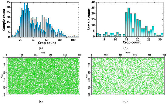
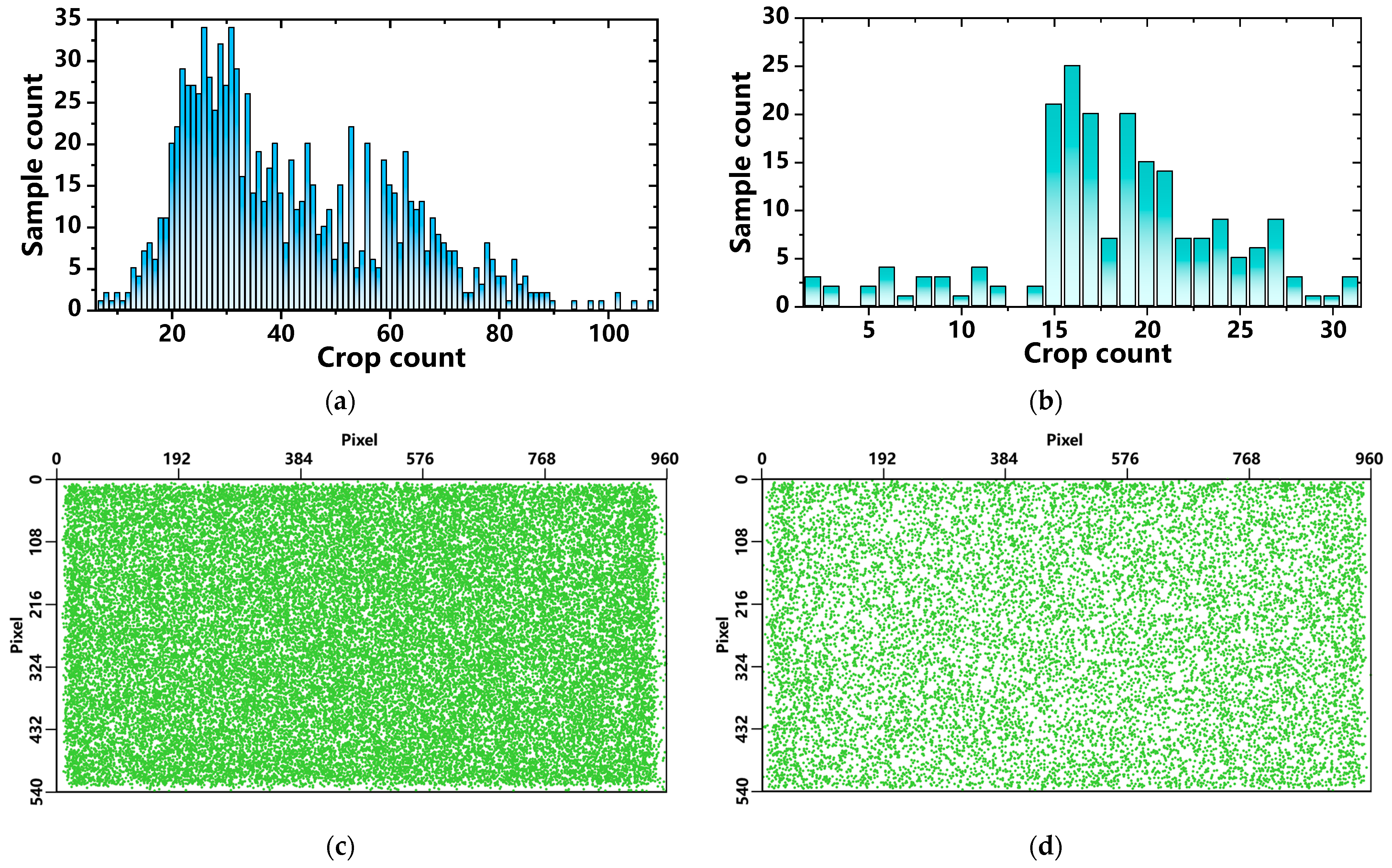
As shown in Figure 1a,b, the wheat dataset exhibits a wider range of target counts per image and presents a clear long-tail distribution. This indicates that the dataset contains not only a large number of medium- and high-density samples, but also a small number of extremely dense scenes. Such a distribution can effectively simulate real field conditions characterized by dense spike distributions, occlusion, and overlap, thereby providing a suitable benchmark for evaluating the model’s ability in small-object detection and dense-target discrimination. In contrast, the rice dataset shows a more concentrated target-count distribution, with most samples falling within the interval of [15], while still retaining a small number of low-density and high-density samples. This ensures a relatively stable overall distribution while preserving a certain level of scene diversity.

To further evaluate the spatial balance of target distributions in the datasets, the center point of each target was extracted and normalized to a unified scale of 960 pixels × 540 pixels, based on which label distribution scatter plots were generated. Figure 1c,d show that the target distributions in both the wheat and rice datasets are generally well balanced, which helps the model learn multidimensional crop features across different spatial locations and thereby improves detection and counting performance.

2.2. The Design Principle of YOLO-DC

2.2.1. YOLOv12

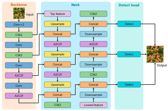
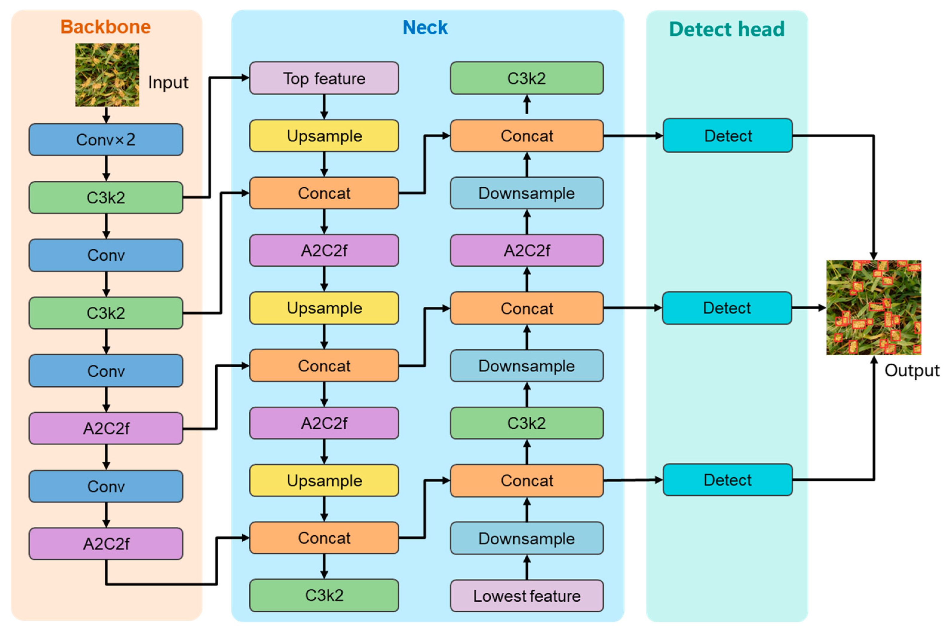
YOLOv12 is an attention-based real-time object detection algorithm jointly developed by the research teams from the University at Buffalo, State University of New York, and the University of Chinese Academy of Sciences [21]. The model family includes five variants of different scales, namely Nano, Small, Medium, Large, and Xlarge, making it adaptable to deployment scenarios with different computational resources. As shown in Figure 2, YOLOv12 mainly consists of three components: the Backbone, Neck, and Detection head. Specifically, the Backbone adopts the Residual efficient layer aggregation network (R-ELAN) structure and integrates the Area Attention (A2) module, 7 × 7 depthwise separable convolution, and FlashAttention, which significantly enhances feature extraction capability while effectively reducing computational complexity. The Neck follows a PAN-FPN bidirectional feature fusion architecture to efficiently integrate feature maps from different levels, while the area attention module helps capture key regional information more precisely, thereby further improving the model’s adaptability and robustness in complex scenes. The Detection head adopts a decoupled design for classification and regression tasks, where the classification branch uses binary cross-entropy (BCE) loss, and the regression branch combines distribution focal loss (DFL) with CIoU loss, enabling joint optimization of classification and bounding box regression.

However, in UAV aerial imaging scenarios, crop targets such as spikes and fruits usually occupy only a small proportion of pixels in the entire image, and their scale is much smaller than that of the background, making them typical dense small objects. In addition, these targets are often characterized by large quantity, small spacing, and dense clustering, so adjacent instances are prone to partial contact, overlap, or occlusion. Furthermore, due to differences in growth stages, crop varieties, and viewing angles, crop targets exhibit considerable intra-class variation in color, texture, shape, and size, which further increases the difficulty of recognition.

As a result of these characteristics, the recognition and counting of crops in UAV aerial images face several major challenges. First, small objects contain limited pixel information, and repeated downsampling in deep networks tends to cause the loss of fine-grained details, which may lead to missed detections and localization errors. Second, dense distribution and mutual occlusion make the boundaries between adjacent targets ambiguous, causing the model to mistakenly merge multiple targets into a single one or produce duplicate detections in local regions. Third, crop targets are often highly similar to background structures such as leaves and stems in terms of color and texture, which easily results in false positives, especially under canopy closure or cluttered background conditions. Therefore, for crop recognition and counting tasks in UAV-based agricultural scenarios, it is essential to improve the model’s ability in fine-grained feature preservation, dense-target separation, boundary representation, and background interference suppression, so as to achieve high-precision object detection and quantitative counting.

2.2.2. YOLO-DC

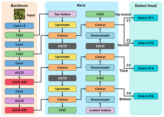
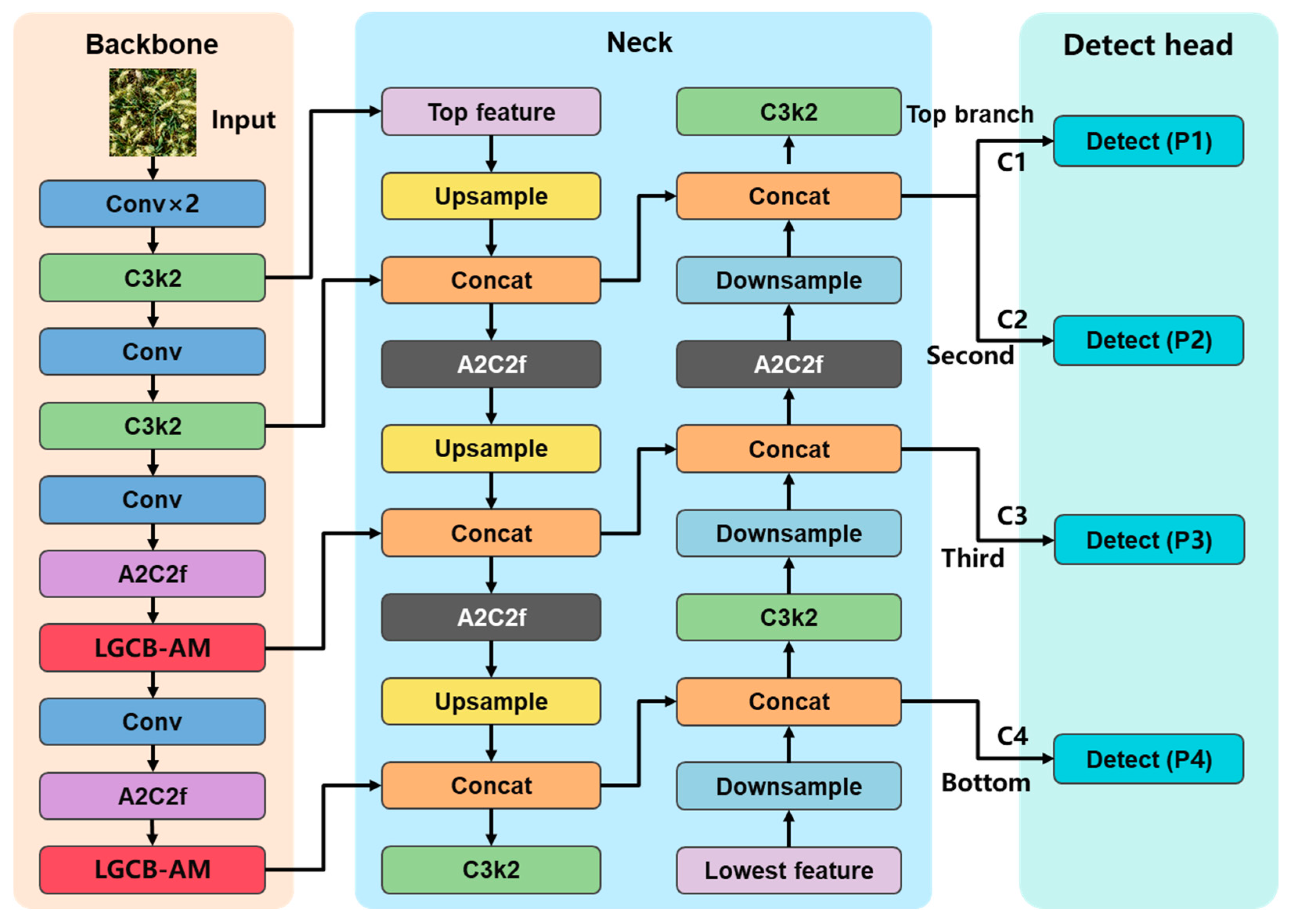
To address the challenges faced by YOLOv12 in agricultural scenarios, such as the low pixel proportion of small targets, large scale variations, and dense target distributions, this study proposes an improved crop detection and counting network based on YOLOv12, named YOLO-DC. The proposed model inherits the basic architecture of YOLOv12 and mainly consists of three components: the Backbone, Neck, and Detection Head, as shown in Figure 3. On this basis, YOLO-DC introduces two key improvement strategies.

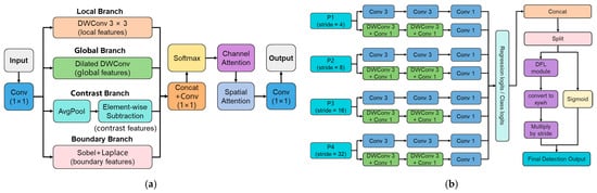
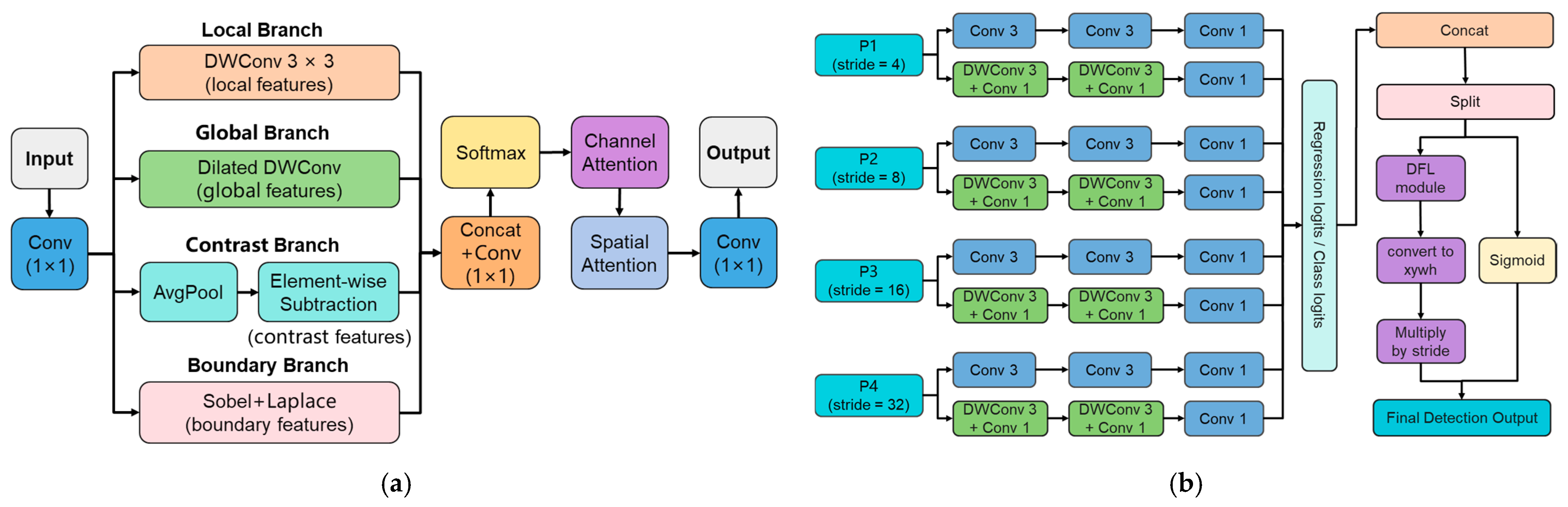
(1) A local–global–contrast–boundary attention mechanism (LGCB-AM) is designed and cascaded after the A2C2f modules in both the Backbone and Neck to enhance the model’s ability to extract local texture, global contextual information, edge and boundary cues, as well as target separation features for small objects (Figure 4a). This module effectively improves the modeling of target contours, adjacent instance boundaries, and foreground—background differences in dense target scenes, thereby strengthening the representation ability and anti-interference capability of the model in complex agricultural environments.

(2) A multi-scale detection head (MS-DH) is further designed to replace the original detection head (Figure 4b). By introducing higher-resolution shallow features, MS-DH effectively compensates for the loss of spatial details in deep features, enabling the network to perceive target contours, boundary differences, and local texture variations at a finer scale. As a result, it improves target recall and reduces missed detections, false detections, and duplicate detections in dense regions. Through these two improvements, YOLO-DC is better suited for crop detection and counting tasks in UAV-based agricultural scenes characterized by small, densely distributed, heavily occluded targets and complex backgrounds.

2.2.3. LGCB-AM

To improve small-object detection and counting accuracy in dense crop scenes such as wheat and rice, this study designs the LGCB-AM module. The novelty of LGCB-AM does not lie in introducing new primitive operators, but in the task-oriented organization and adaptive coordination of existing operators for UAV-based agricultural imagery, where crop targets are often small, densely distributed, boundary-adhered, visually similar to the background, and affected by feature interference between adjacent instances. Specifically, LGCB-AM jointly models local texture, global context, saliency contrast, and boundary responses through a multi-branch structure, and further employs a lightweight gating mechanism to generate input-dependent branch weights according to target density, occlusion degree, and background complexity. Different from a simple parallel aggregation structure, the branch responses are further processed by an input-dependent gating mechanism, which generates spatially adaptive branch weights through a lightweight 1 × 1 convolution and softmax normalization.

Specifically, the input feature F₁ is first processed by LayerNorm, a 1 × 1 convolution layer, and a Value feature mapping, as defined in Equation (1). The refined feature is then fed in parallel into four complementary branches, which are responsible for extracting neighborhood texture information, contextual information with an enlarged receptive field, regional saliency information, and edge response information, respectively. These branch features are further combined with a gating region to generate three types of guidance signals, namely center, boundary, and repulsion signals. Finally, fine-grained feature representation is achieved through weighted fusion and output enhancement.

Among them, the local branch employs a 3 × 3 depthwise separable convolution to capture local textures and neighborhood details of crop targets, thereby improving the fine-grained representation capability for small objects, as defined in Equation (2). The global branch adopts a dilated depthwise convolution to enlarge the receptive field and model wider spatial dependencies, thus enhancing the understanding of group distribution patterns and complex backgrounds, as defined in Equation (3). The contrast branch highlights salient target regions by measuring the difference between local features and contrast statistical information, thereby improving the discriminability between foreground targets and the background, as defined in Equation (4). The boundary branch combines Sobel and Laplace operators to extract edge and contour information, which strengthens boundary responses between adjacent targets and alleviates adhesion and occlusion issues, as defined in Equation (5). Furthermore, the repulsion-gating branch S_r generates separation cues by utilizing center, boundary, and crowding information, thereby suppressing feature mixing among adjacent targets and improving dense target discrimination, as defined in Equation (6).

$$F_2=W\times C_1(\mathrm{LN}(F_1)),$$

(1)

$$F_3={\mathrm{DWC}}_3(F_2),$$

(2)

$$F_4={\mathrm{DWC}}_3^d(F_2),$$

(3)

$$F_5=F_2-B(\mathrm{GAP}(F_2)),$$

(4)

$$F_6=\mathrm{Sobel}(F_2)+\mathrm{Laplace}(F_2),$$

(5)

$$S_r=\sigma \left(\alpha D_{pc}+\beta \rho \right),$$

(6)

where F₁∈R^C×H×W; LN is LayerNorm; C₁ is convolution layer with kernel 1; W represents a linear mapping parameter; DWC₃ represents a depthwise separable convolution layer with kernel 3; DWC^d₃ represents the convolution layer of cavity depth with expansion rate d; GAP stands for global average pooling; B represents expanding the channel vector to the same space size as F₂; Sobel and Laplace represent the edge responses of Sobel and Laplace operators respectively; σ represents Sigmoid function; D_pc denotes the local peak-to-center response gap computed from the center-response map; ρ represents the crowd score, obtained by performing 5 × 5 average pooling on the center-response map; and α and β are weight coefficients.

To obtain the adaptive fusion weights, the four branch features are first concatenated along the channel dimension and then fed into a lightweight branch-gating layer implemented by a 1 × 1 convolution. This layer produces four input-dependent logit maps, denoted as z_i, corresponding to the local, global, contrast and boundary branches, respectively. Therefore, z_i is not a fixed learnable scalar or a manually computed pooled statistic, but a spatially adaptive response predicted from the branch features. The normalized branch weights are then obtained by applying the softmax operation along the branch dimension. Furthermore, each branch feature is fused by softmax adaptive weighting, as defined by Equations (7) and (8). Under this operation, the model can adaptively adjust the importance of different branches according to the input.

$${\lambda }_i={\displaystyle \frac{\exp \left(z_i\right)}{{\displaystyle \sum _{j=3}^6\exp }\left(z_j\right)}},$$

(7)

$$F_f={\lambda }_3{F}_3+{\lambda }_4{F}_4+{\lambda }_5{F}_5+{\lambda }_6{F}_6,$$

(8)

where z_i is weight response of each branch; F_f is mixed feature of four branches.

Finally, the channel and space are enhanced by combining space gating and channel gating, so as to obtain the output characteristics, thus providing clearer and more stable discrimination information for the subsequent detection heads, as defined by Equation (9).

$$F_7=C_1\left(SAM\left(CAM\left(F_f\right)\right)\right)$$

(9)

where SAM is space gating; CAM is channel gating; and F₇ is the output of the LGCB-AM.

2.2.4. Multi-Scale Detection Head (MS-DH)

The original YOLOv12 detection head mainly relies on feature maps after multiple downsampling operations. Although these features contain rich semantic information, their relatively low spatial resolution may lead to the loss of fine-grained edge, texture, and positional information for dense small crop targets. As a result, problems such as missed detections, localization errors, and duplicate counting in dense regions may occur. This limitation becomes more pronounced when adjacent spikes are closely spaced and severely adhered, since low-resolution detection features may weaken subtle spatial differences between neighboring targets, resulting in inadequate perception of dense small objects.

To address these issues, a Multi-Scale Detection Head (MS-DH) is designed in this study. MS-DH adopts a four-scale decoupled detection structure (P1–P4), in which independent detection branches are constructed for four feature maps from the feature fusion network, corresponding to strides of 4, 8, 16, and 32, respectively, and the four branches use the same architectural template but have independent learnable parameters. Specifically, the backbone produces four feature maps, denoted as C1, C2, C3, and C4, with strides of 4, 8, 16, and 32 relative to the input image, respectively. The highest-resolution detection feature P1 is not directly taken from the shallow backbone output. Instead, it is generated in the neck by fusing shallow spatial information and top-down semantic information. First, C4 is upsampled and concatenated with C3 to form a top-down fusion feature. This feature is further upsampled and fused with C2. Finally, the resulting feature is upsampled again and concatenated with the shallow C1 feature, followed by a C3k2 fusion block to obtain P1 with a stride of 4.

Based on P1, the remaining detection features are constructed through a bottom-up path aggregation network style fusion pathway. P1 is downsampled and concatenated with the corresponding top-down feature to generate P2 with a stride of 8. Then, P2 is downsampled and fused with a higher-level neck feature to generate P3 with a stride of 16. Finally, P3 is downsampled and fused with the deepest semantic feature C4 to generate P4 with a stride of 32. Therefore, the proposed MS-DH takes P1, P2, P3, and P4 as detection inputs, corresponding to four detection branches with strides of 4, 8, 16, and 32, respectively.

At each scale, the detection head follows a decoupled strategy, in which object localization and category prediction are modeled separately. Specifically, the input feature is first divided into two parallel branches. The regression branch consists of two convolution layers with a kernel size of 3 and one convolution layer with a kernel size of 1, and is used to predict the discrete distribution parameters of bounding boxes, with an output channel number of 4 × reg_max, where reg_max is 16. The classification branch is composed of two groups of alternating DWConv and pointwise convolutions (1 × 1 Conv), followed by a final 1 × 1 convolution for category prediction, with an output channel number equal to the number of classes n_c. The outputs of the two branches are concatenated along the channel dimension to form a joint prediction representation. It should be noted that the detection branches at different scales do not share convolutional weights. This scale-specific parameter design allows each branch to adapt to different spatial resolutions and semantic levels.

During the prediction decoding stage, the concatenated output is first split into a regression part and a classification part. For the regression branch, a Distribution Focal Loss (DFL) integral module is used to integrate the discrete distribution into continuous bounding box offsets, which are then converted into the (x, y, w, h) format using the dist2bbox function and further scaled according to the stride of the corresponding feature level. For the classification branch, category probabilities are obtained through the Sigmoid function. Finally, the decoded bounding boxes and classification probabilities from P1, P2, P3, and P4 are concatenated to generate the final multi-scale detection results.

For a 1024 × 1024 input image, the stride-4, stride-8, stride-16, and stride-32 branches produce 65,536, 16,384, 4096, and 1024 prediction locations, respectively. Therefore, the four-scale head produces 87,040 prediction locations in total, whereas a conventional three-scale head produces 21,504 prediction locations. This analysis shows that the stride-4 branch improves small-object recall and boundary-sensitive localization, but also increases prediction density, high-resolution computation, memory access, and post-processing cost.

2.2.5. Evaluation Metrics

To evaluate the performance of YOLO-DC, seven commonly used metrics were adopted: precision (P), recall (R), mAP50, mAP50–95, mean absolute error (MAE), root mean square error (RMSE), and coefficient of determination (R²). Among them, the P is used to measure the proportion of correctly predicted positive samples among all samples predicted as positive by the model, as defined in Equation (10). The R measures the proportion of true positive samples that are correctly detected by the model, as defined in Equation (11). mAP50 is a widely used comprehensive metric in object detection, representing the mean average precision of all categories at an IoU threshold of 0.5, as defined in Equation (12). mAP50–95 Here, AP denotes the area under the precision–recall curve for a specific category.

In addition, MAE is employed to evaluate the average absolute difference between the predicted values and the ground-truth values, as defined in Equation (14). For the counting evaluation, the predicted count was obtained directly from the final detection results after post-processing rather than from an additional regression branch. Specifically, for the (i)-th image, all predicted boxes with confidence scores lower than the confidence threshold (${\tau }_{\mathrm{c}\mathrm{o}\mathrm{n}\mathrm{f}}$) were first discarded. Then, non-maximum suppression (NMS) was applied to the remaining boxes using an NMS IoU threshold (${\tau }_{\mathrm{n}\mathrm{m}\mathrm{s}}$). The predicted count ${\widehat{y}}_i$ was defined as the number of bounding boxes retained after confidence filtering and NMS, as defined in Equation (15). RMSE is used to measure the overall dispersion of prediction errors, as defined in Equation (16).

$$P={\displaystyle \frac{TP}{TP+FP}}$$

(10)

$$R={\displaystyle \frac{TP}{TP+FN}}$$

(11)

$$\mathrm{mAP}50={\displaystyle \frac{1}{N}}{\displaystyle \sum _{i=1}^{N}A{P}_i}$$

(12)

$$\mathrm{mAP}50-95={\displaystyle \frac{1}{10N}}{\displaystyle \sum _{i\in \{0.5,0.55,\dots ,0.95\}}^{N}A{P}_i}$$

(13)

$$\mathrm{MAE}={\displaystyle \frac{1}{n}}{\displaystyle \sum _{i=1}^n\left|y_i-{\widehat{y}}_i\right|}$$

(14)

$${\widehat{y}}_i=\left|D_i^{NMS}\left({\tau }_{conf},{\tau }_{nms}\right)\right|$$

(15)

$$\mathrm{RMSE}=\sqrt{{\displaystyle \frac{1}{n}}{\displaystyle \sum _{i=1}^n{\left(y_i-{\widehat{y}}_i\right)}^2}}$$

(16)

where TP denotes the number of correctly predicted positive samples; FP denotes the number of samples predicted as positive but actually negative; FN denotes the number of positive samples that fail to be correctly detected; N denotes the number of categories; n denotes the number of samples; y_i denotes the ground-truth count of the i-th image; $\widehat{y_i}$ denotes the predicted count obtained from the retained post–NMS detections of the i-th image; and ${\mathit{D}}_i^{NMS}$ denotes the final set of retained detections for the (i)-th image.

2.3. Comparison Experiments

To comprehensively evaluate the performance of YOLO-DC in UAV-based crop counting tasks, several representative deep learning models were selected as comparison methods, including Faster R-CNN [22], RetinaNet [23], SSD300 [24], FCOS [25], SSDLite320 [26], D-Fine [27], DETR [28], CS-Net [29], HeadCount [30], YOLOv10 [31], YOLOv12 [21], and YOLOv26 [32]. Among them, YOLOv10, YOLOv12, and YOLOv26 represent recent models from the YOLO family. CS-Net and HeadCount were included as recent non-YOLO crop-counting-specific baselines. Unlike general-purpose detection models, these methods are more directly related to dense agricultural counting tasks and therefore provide a task-relevant comparison for evaluating the counting ability of YOLO-DC under dense small-object scenarios. All models were trained, validated, and tested under the same data partition protocol to ensure the fairness and comparability of the experimental results.

Figure 1a shows that the number of wheat ears varies substantially across different samples in the wheat dataset. To further investigate the influence of target density on the detection and counting performance of YOLO-DC, an additional experiment was conducted with target density as the independent variable. According to the density distribution shown in Figure 1a, the test samples were divided into four density groups, with density ranges of ≤27, 28–37, 38–60, and ≥61, respectively. Each group contained 25 samples, all of which were selected from the test set.

In terms of implementation, all models were trained and evaluated on an NVIDIA GeForce RTX 4090 GPU, using PyTorch 2.3.0 and Python 3.12, with CUDA 12.3 for accelerated computation. For all models, the hyperparameter settings were configured as follows to ensure a fair comparison. Except for SSD300 and SSDLite320, which used input resolutions of 300 × 300 and 320 × 320, respectively, all other models were trained with an input size of 1024 × 1024. The number of training epochs was uniformly set to 100, and the batch size was fixed at 4 for all models. In terms of optimization, Faster R-CNN, RetinaNet, SSD300, FCOS, and SSDLite320 were trained using the SGD optimizer with an initial learning rate of 1 × 10⁻⁴, whereas the remaining models, including DETR, D-FINE, CS-Net, HeadCount, YOLOv10, YOLOv12, YOLOv26, and the proposed YOLO-DC, were trained using the AdamW optimizer with the same initial learning rate of 1 × 10⁻⁴. The optimal threshold combination was selected on the validation set according to the counting performance, with MAE used as the primary criterion and RMSE used as the secondary criterion when multiple threshold combinations yielded the same or very similar MAE values. The detection metrics, including mAP50 and mAP50-95, were used only for reporting detection performance and were not involved in the threshold selection procedure. To ensure a fair and systematic post-processing protocol, a validation-set-based threshold search was conducted for each detection-based model within the same broad search space. Specifically, the confidence threshold (τ_conf) was searched from 0.01 to 0.60, and the NMS IoU threshold (τ_nms) was searched from 0.30 to 0.75.

For YOLOv12 and its improved variants, the training process was optimized using a composite detection loss function, which consists of three components: the bounding box regression loss L_box, the classification loss L_cls, and the distribution focal loss L_dfl, as defined in Equation (17). Specifically, L_box denotes the CIoU-based bounding box regression loss, as defined in Equation (18); L_cls denotes the binary cross-entropy (BCE)-based classification loss, as defined in Equation (19); and L_dfl denotes the Distribution Focal Loss (DFL), as defined in Equation (20).

$$L={\lambda }_{box}{L}_{box}+{\lambda }_{cls}{L}_{cls}+{\lambda }_{dfl}{L}_{dfl}$$

(17)

$$L_{box}={\displaystyle \frac{1}{N_{pos}}}{\displaystyle \sum _{i=1}^{N_{pos}}\left(1-\mathrm{CIoU}(b_i,{\widehat{b}}_i)\right)}$$

(18)

$$L_{cls}={\displaystyle \frac{1}{N_{pos}}}{\displaystyle \sum _{i=1}^{N_{pos}}\mathrm{BCE}}(s_i,{\widehat{s}}_i)$$

(19)

$$L_{dfl}={\displaystyle \frac{1}{N_{pos}}}{\displaystyle \sum _{i=1}^{N_{pos}}\mathrm{DFL}}(d_i,{\widehat{d}}_i)$$

(20)

where λ_box, λ_cls and λ_dfl represent the weight coefficient of the corresponding loss term, respectively; N_pos is the number of positive samples; b_i and $\widehat{{\mathit{b}}_{\mathit{i}}}$ respectively represent the true boundary box and the predicted boundary box of the ith positive sample; CIoU is complete intersection over union; s_i and $\widehat{{\mathit{s}}_{\mathit{i}}}$ represent the true category label and predicted category score of the i-th positive sample, respectively; BCE stands for Binary Cross Entropy Loss; d_i and $\widehat{{\mathit{d}}_{\mathit{i}}}$ respectively represent the true position distribution and the predicted position distribution of the i-th positive sample; DFL stands for Distribution Focal Loss; and N represents the number of samples in the test set.

2.4. Ablation Experiments

To investigate the structural rationality of YOLO-DC, ablation studies were conducted from three perspectives: the core components of YOLO-DC, the insertion positions of the LGCB-AM, and the internal feature extraction branches of LGCB-AM. In all ablation experiments, YOLO-DC was used as the baseline model.

2.4.1. Ablation Experiment 1: Core Component Analysis

The core components of YOLO-DC mainly include the LGCB-AM and the MS-DH. To evaluate the contribution of these two components to the proposed network, the first group of ablation experiments was designed as follows:

Model 1–1: YOLO-DC used the original detection head of YOLOv12 replace the MS-DH;

Model 1–2: YOLO-DC deleted the LGCB-AM;

Model 1–3: YOLO-DC used the original detection head of YOLOv12 replace the MS-DH and deleted the LGCB-AM.

2.4.2. Ablation Experiment 2: Insertion Position of LGCB-AM

To determine the optimal insertion position of the LGCB-AM within YOLOv12, a second group of ablation experiments was conducted by embedding the module at different feature extraction and fusion stages. The specific settings are described as follows:

Model 2–1: YOLO-DC with the LGCB-AM inserted at C3k2;

Model 2–2: YOLO-DC with the LGCB-AM inserted between Backbone and Neck;

Model 2–3: YOLO-DC with the LGCB-AM inserted between Neck and Detect head;

Model 2–4: YOLO-DC with the LGCB-AM inserted at C3k2 and A2C2f.

2.4.3. Ablation Experiment 3: Branch-Wise Analysis of LGCB-AM

To further analyze the contribution of different functional branches within the LGCB-AM, a third group of ablation experiments was designed. In this group, the local branch, global branch, contrast branch, and boundary branch were removed one by one to evaluate their respective effects on detection and counting performance. The specific settings are described as follows:

Model 3–1: YOLO-DC without the local branch;

Model 3–2: YOLO-DC without the global branch;

Model 3–3: YOLO-DC without the contrast branch;

Model 3–4: YOLO-DC without the boundary branch.

2.5. Transfer Experiments

To evaluate the cross-crop transfer potential of YOLO-DC in crop counting tasks, transfer experiments were conducted on the rice dataset. First, DETR, YOLOv12, and YOLOv26, which achieved relatively strong performance in previous experiments, were selected as comparison models. Specifically, each model was first pretrained on the wheat dataset for 100 epochs and then fine-tuned on the training subset of the rice dataset for 20 epochs. Meanwhile, to ensure the same total number of training epochs, a control experiment based on random initialization was conducted, in which each model was trained from scratch on the same rice training subset for 120 epochs. This setting was used to systematically compare the performance differences between pretrained transfer and random-initialization training in detection and counting tasks.

3. Results

3.1. Results and Analysis of Comparison Experiments

3.1.1. Results of Different Model in Wheat Dataset

Table 1. Results of comparison experiments.

Model	Params (M)	p	R	mAP50	mAP50-95	MAE	RMSE	R2
Faster R-CNN	41.352	0.924	0.848	0.889	0.494	3.27	5.057	0.923
DETR	41.502	0.926	0.889	0.909	0.519	3.67	5.043	0.924
RetinaNet	32.222	0.909	0.824	0.851	0.467	4.20	6.211	0.885
SSD300	23.746	0.882	0.803	0.833	0.437	5.12	7.732	0.821
FCOS	32.118	0.896	0.844	0.892	0.495	5.96	8.540	0.781
D-FINE	3.720	0.701	0.794	0.682	0.331	10.82	22.421	0.624
SSDLite	2.207	0.617	0.678	0.523	0.283	13.07	15.251	0.573
CSNet	94.313	-	-	-	-	6.79	9.077	0.735
HeadCount	26.678	-	-	-	-	7.96	10.100	0.695
YOLOv10	2.707	0.888	0.840	0.919	0.561	5.19	7.862	0.815
YOLOv12	2.520	0.916	0.846	0.929	0.558	3.65	5.237	0.917
YOLOv26	2.504	0.905	0.854	0.930	0.560	3.28	4.775	0.932
YOLO-DC	2.731	0.910	0.871	0.934	0.567	3.02	4.470	0.939

shows that YOLO-DC demonstrates the best overall performance among all compared models. Although its parameter count is only 2.731 M, which is far lower than that of heavy detectors such as Faster R-CNN, DETR, and RetinaNet, it achieves the best results in mAP50, mAP50–95, MAE, RMSE, and R², reaching 0.934, 0.567, 3.02, 4.47, and 0.939, respectively. These results indicate that the proposed method not only provides higher detection accuracy but also achieves more accurate and stable counting performance. Compared with the original YOLOv12, YOLO-DC improves mAP50-95 by 0.009, while reducing MAE and RMSE by approximately 17.3% and 14.6%, respectively. Compared with YOLOv26, YOLO-DC further improves mAP50-95 and R² while obtaining lower counting errors. These findings demonstrate that YOLO-DC achieves a better trade-off between lightweight design, detection accuracy, and counting robustness.

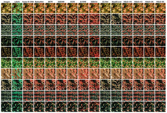
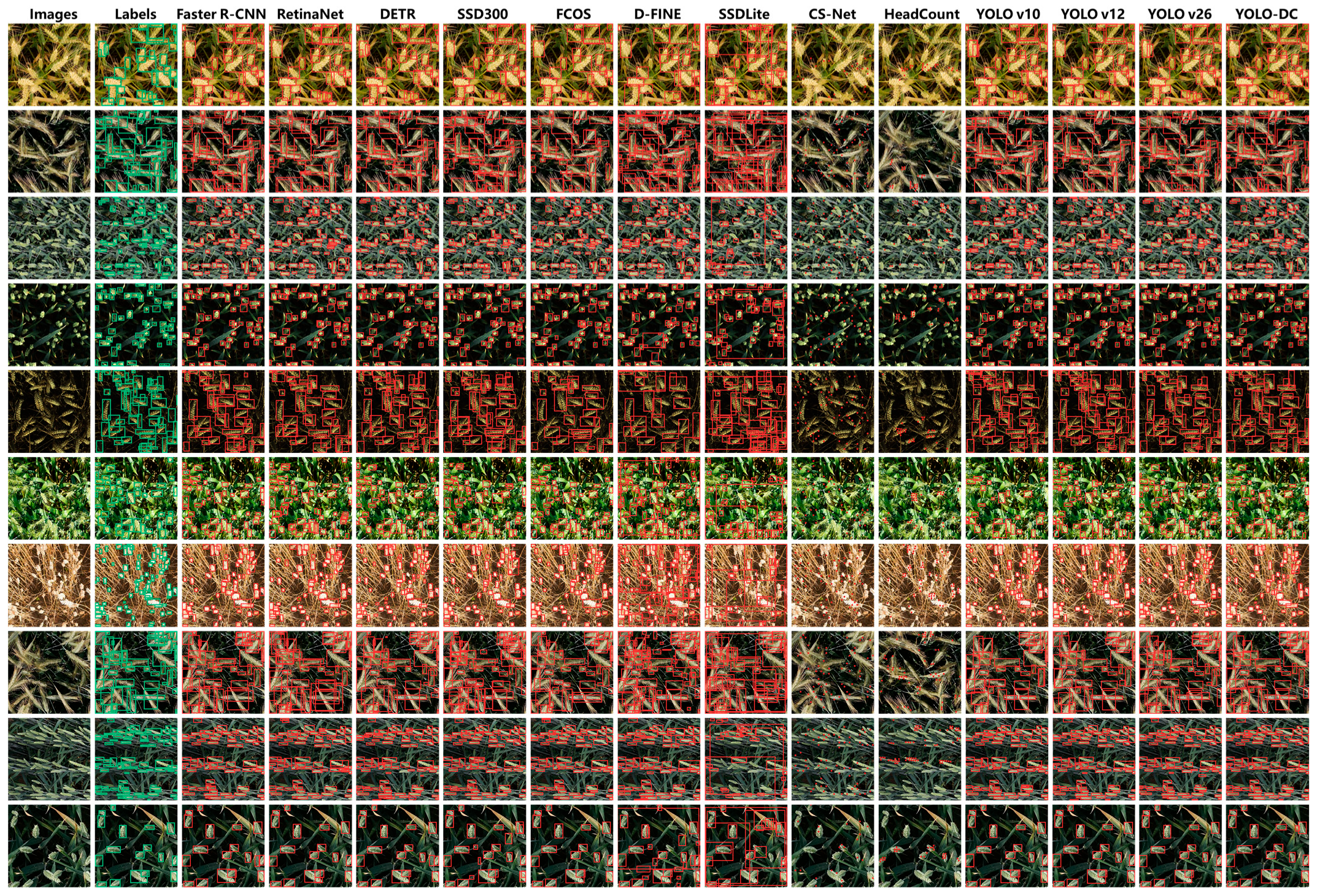
As shown in Figure 5, YOLO-DC demonstrates more stable detection performance in complex agricultural scenes, with particularly notable advantages in samples characterized by dense distribution, small objects, severe occlusion, and strong background interference. The detection visualizations show that YOLO-DC achieves a higher degree of correspondence between predicted boxes and ground-truth targets, maintaining more complete target coverage in dense regions while effectively reducing missed detections, duplicate detections, and false positives caused by background noise. In contrast, some classical or lightweight models are more prone to target adhesion, partial target omission, and increased false alarms in challenging areas.

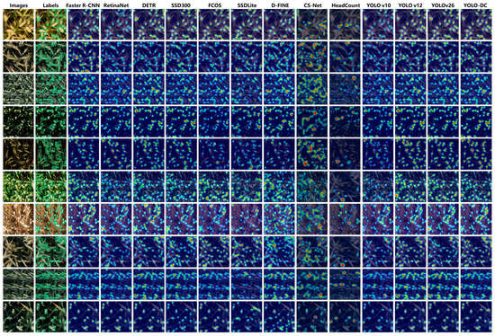
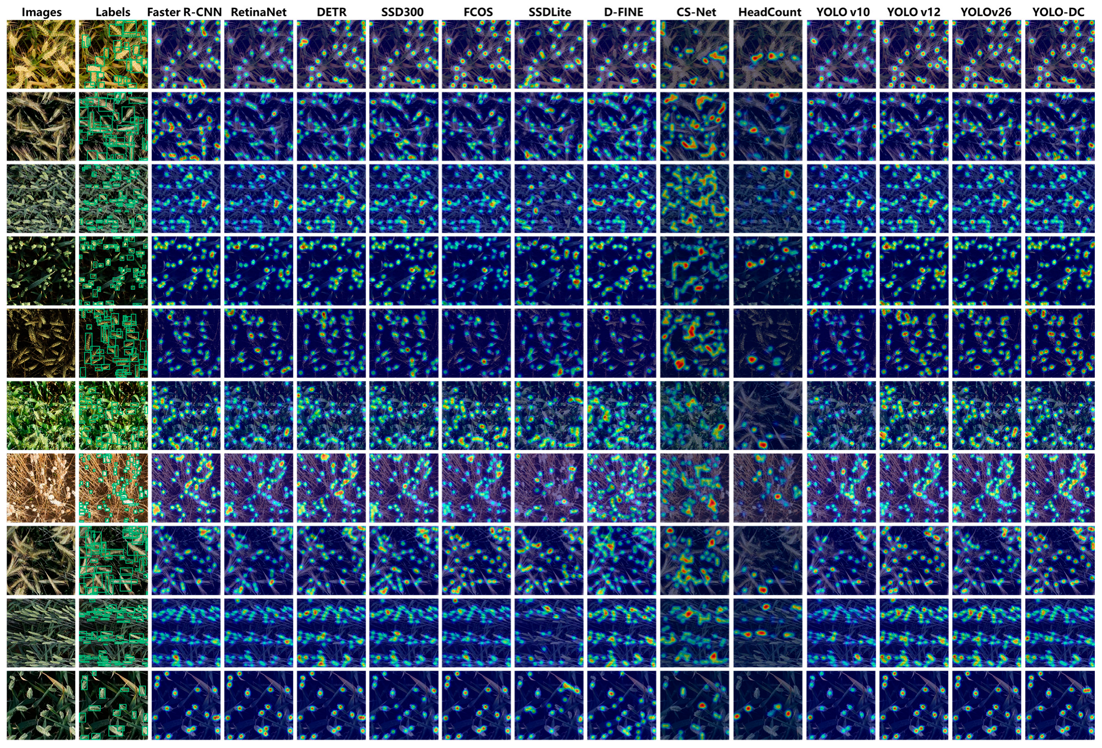
Furthermore, the high-response regions of YOLO-DC are more concentrated on the crop targets themselves, while responses to non-target background regions are significantly suppressed, indicating that the proposed model is able to focus more accurately on key target areas and possesses stronger target representation and anti-interference capabilities (Figure 6). Overall, YOLO-DC exhibits superior performance in small-object recognition, dense-target discrimination, and adaptation to complex scenes, thereby providing a more reliable detection foundation for subsequent high-precision crop counting and yield prediction.

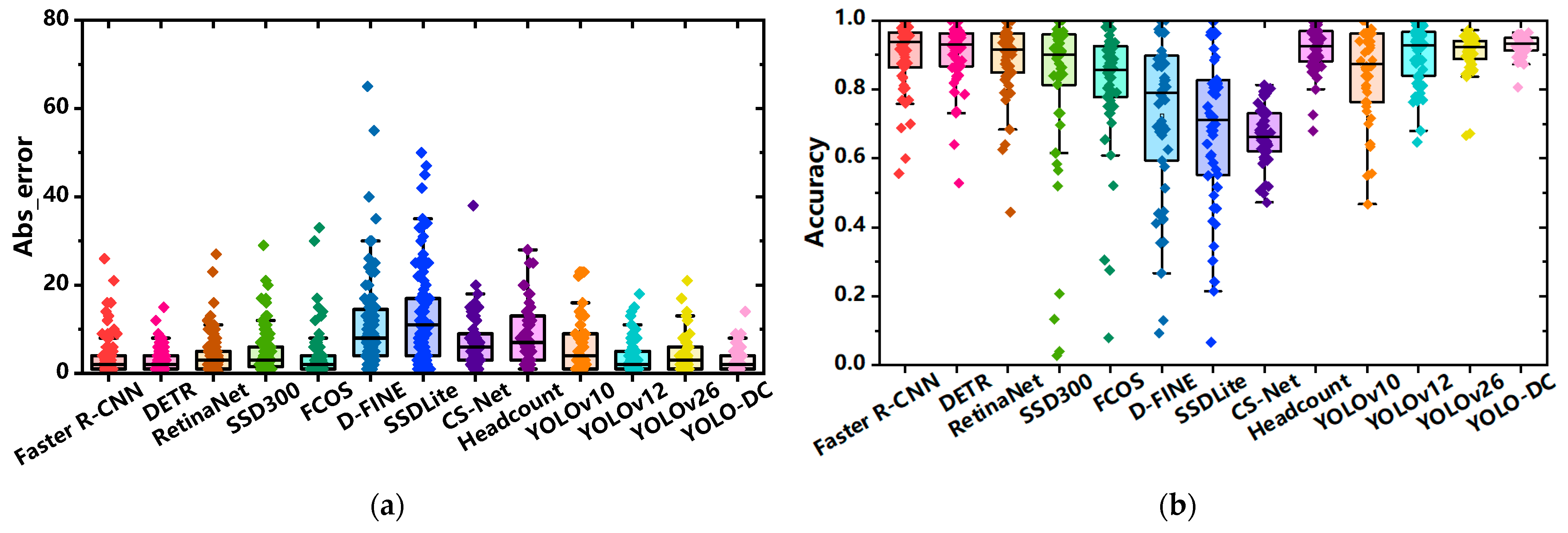
The boxplot results (Figure 7) show that YOLO-DC has a lower median and smaller variation range in absolute error, while exhibiting a higher and more stable distribution in accuracy, indicating that the model not only performs better on average but is also more adaptable and stable across different samples and complex scenarios. Overall, YOLO-DC shows clear advantages in dense small-object detection, complex background suppression, and high-precision counting.

3.1.2. Results and Analysis of Different Density for YOLO-DC

As shown in

Table 2. Results of YOLO-DC under different density dataset.

Density	Count Range	Images	Instances	AP50	mAP50:95	MAE	RMSE
Low-density	≤27	25	568	0.950	0.591	2.12	2.67
Medium-density	28–37	25	779	0.955	0.572	1.88	2.57
High-density	38–60	25	1183	0.917	0.568	4.68	5.71
Very high-density	≥61	25	1703	0.938	0.578	4.16	5.89

, YOLO-DC maintains strong detection capability and reasonable robustness across samples with different density levels. Overall, the model performs most stably in the low-density and medium-density groups, with the medium-density group achieving the best overall counting performance, including the highest AP50 (0.955) and the lowest MAE (1.88) and RMSE (2.57). This indicates that YOLO-DC can achieve highly accurate detection and counting when the target number is moderate and occlusion is relatively limited. As the target density further increases to the high-density and very high-density groups, the counting errors become more pronounced, suggesting that dense distribution, boundary adhesion, and mutual occlusion impose greater challenges on quantity estimation. Nevertheless, even under the very high-density condition, YOLO-DC still maintains an AP50 of 0.938 and an mAP50:95 of 0.578, demonstrating that the model retains strong object localization and recognition capability even in extremely crowded scenes. In general, YOLO-DC shows good adaptability to crop samples of varying densities, although its counting performance is still affected to some extent as target density increases.

3.2. Results and Analysis of Ablation Experiments

3.2.1. Results and Analysis of Ablation Experiment 1

Table 3. Results of ablation experiment 1.

Model	mAP50-95	MAE	RMSE
Baseline	0.567	3.020	4.470
Model 1-1	0.532	3.263	4.688
Model 1-2	0.510	3.860	4.950
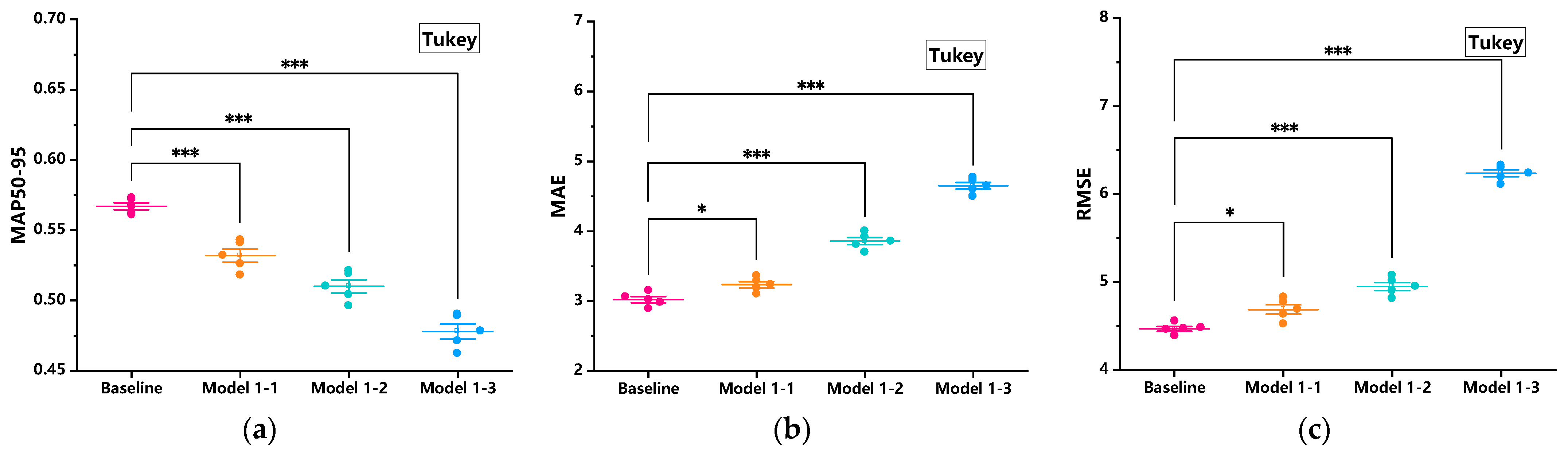
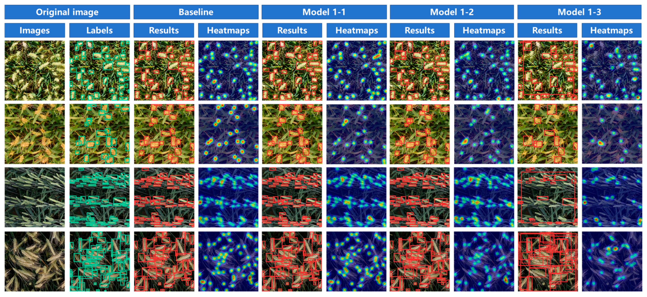
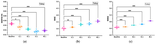
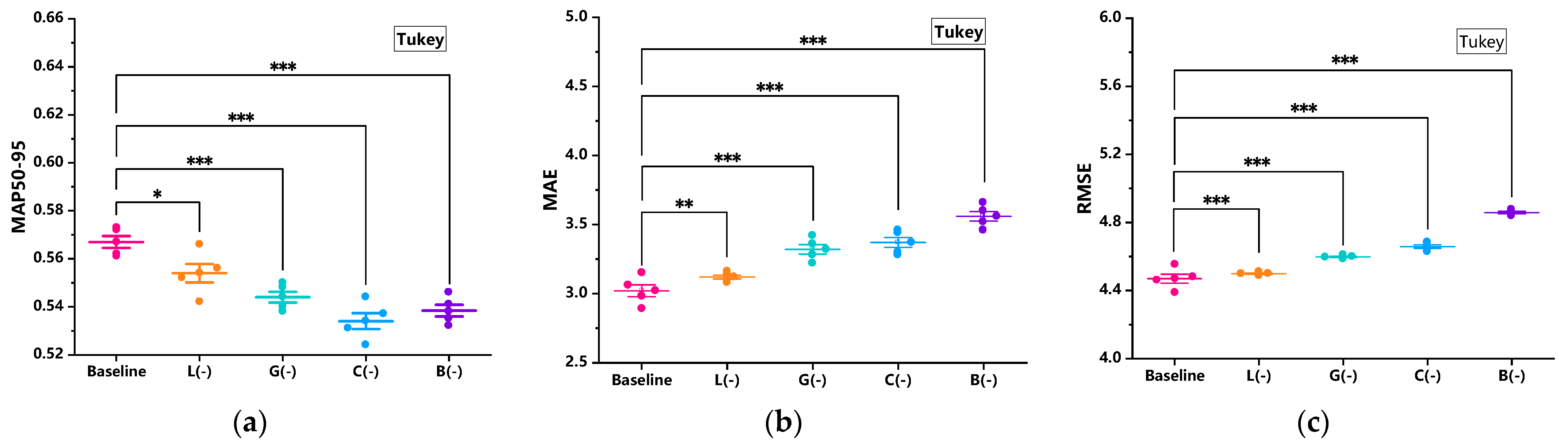
Model 1-3	0.478	4.652	6.237

and Figure 8 indicate that both MS-DH and LGCB-AM make important contributions to the performance improvement of YOLO-DC, and the baseline achieves the best overall performance. Quantitatively, the Baseline reaches 0.567, 3.020, and 4.470 in mAP50-95, MAE, and RMSE, respectively. When MS-DH is replaced with the original YOLOv12 detection head (Model 1–1), the model performance drops noticeably, indicating that MS-DH effectively improves the representation and detection of multi-scale small objects.

By comparison, removing LGCB-AM (Model 1–2) causes more severe degradation, showing that this module plays a more critical role in feature enhancement, background suppression, and dense-instance discrimination. When both MS-DH and LGCB-AM are removed simultaneously (Model 1–3), the model performs the worst, further demonstrating the strong complementary effect of the two components. The significance analysis also confirms that the Baseline differs significantly from all ablated variants in terms of mAP50-95, MAE, and RMSE, with Model 1–3 showing the largest degradation.

Figure 9 shows that the baseline provides more complete target coverage in dense regions, with predicted boxes better aligned with the ground-truth annotations and fewer missed or duplicate detections. Its heatmaps also show more concentrated high-response regions on the crop targets, indicating stronger target-focusing capability. In contrast, Model 1–1 produces more missed detections in locally dense areas, suggesting insufficient small-object detail representation without MS-DH. Model 1–2 shows more dispersed heatmap responses and increased invalid activations in background regions, indicating that LGCB-AM plays an important role in foreground enhancement and background suppression. Model 1–3 performs the worst in both detection and heatmap visualization, with the least concentrated target responses and the most severe false and missed detections. Overall, MS-DH mainly improves the detection of small and multi-scale targets, whereas LGCB-AM is more responsible for enhancing target representation and dense-target separation; together, they form the core basis for the performance gains of YOLO-DC.

3.2.2. Results and Analysis of Ablation Experiment 2

Table 4. Results of ablation experiment 2.

Model	mAP50–95	MAE	RMSE
Baseline	0.567	3.020	4.470
Model 2-1	0.532	3.190	4.698
Model 2-2	0.557	3.060	4.583
Model 2-3	0.513	3.350	4.884
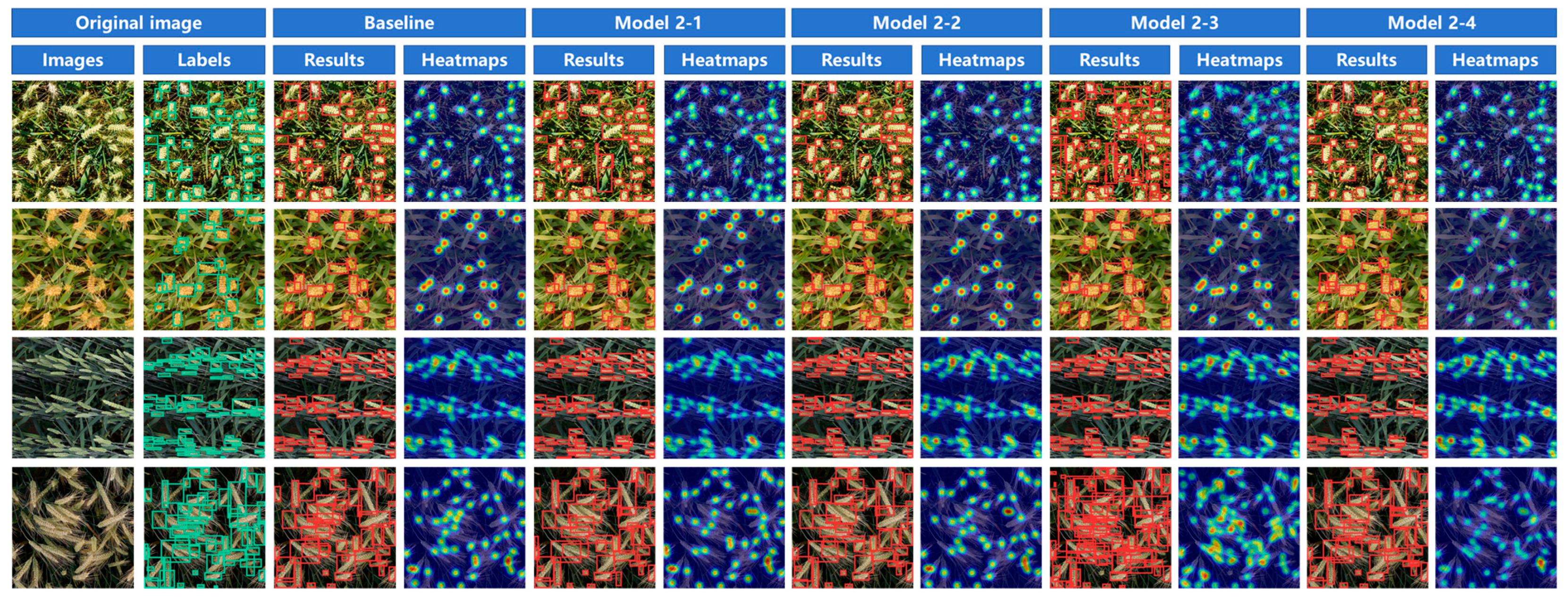
Model 2-4	0.499	3.610	4.943

shows that the Baseline achieves the best overall performance, with mAP50–95, MAE, and RMSE reaching 0.567, 3.020, and 4.470, respectively. This indicates that the current placement strategy of LGCB-AM provides the best balance between detection accuracy and counting stability. In comparison, Model 2–2 performs closest to the Baseline, suggesting that inserting LGCB-AM between the Backbone and Neck can still effectively enhance feature representation. By contrast, Model 2–1, Model 2–3, and Model 2–4 all exhibit more pronounced performance degradation. In particular, Model 2–4 shows the largest decline, with mAP50–95 dropping to 0.499 and MAE and RMSE increasing to 3.610 and 4.943, respectively. These results indicate that injecting LGCB-AM at multiple positions disrupts the original balance of feature transmission and fusion, thereby weakening the overall model performance.

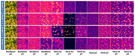
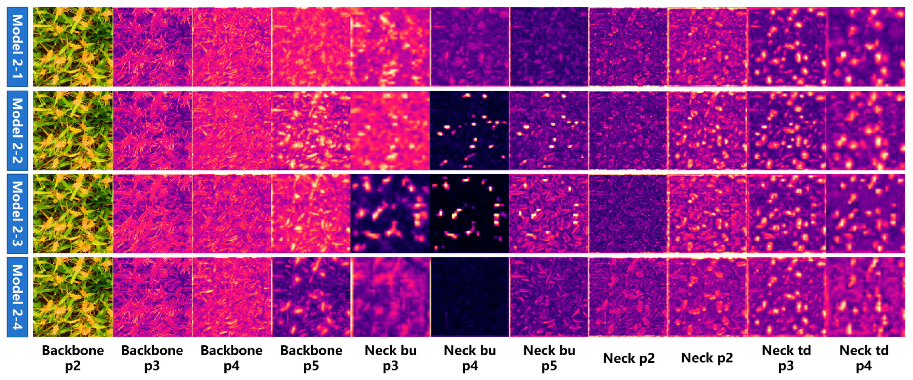
As shown in Figure 10, the Baseline achieves the most accurate correspondence between the predicted boxes and the annotated targets, with more complete target coverage in dense regions and the fewest missed and false detections. Its heatmaps and feature responses are also more concentrated on the crop targets themselves, while invalid activations in background regions are effectively suppressed, reflecting stronger target-focusing and background-suppression capabilities (Figure 11). In contrast, the other variants exhibit more dispersed responses, insufficient activation of local targets, or increased background interference in some samples, with these issues being particularly evident in Model 2–3 and Model 2–4. Overall, these results further confirm that the current insertion position of LGCB-AM in YOLO-DC is the most reasonable design choice, achieving the best balance between high-level semantic enhancement and multi-scale feature fusion.

3.2.3. Results and Analysis of Ablation Experiment 3

As shown in

Table 5. Results of ablation experiment 3.

Model	mAP50–95	MAE	RMSE
Baseline	0.567	3.020	4.470
Model 3-1	0.554	3.120	4.499
Model 3-2	0.544	3.320	4.598
Model 3-3	0.534	3.370	4.657
Model 3-4	0.548	3.560	4.858

, all four branches in LGCB-AM contribute positively to the overall performance, and the complete model achieves the best comprehensive results. Removing the local branch leads to only a slight performance drop, suggesting that this branch mainly supplements fine-grained texture and local structural details of crop targets, thereby providing auxiliary enhancement for small-object representation. In contrast, removing the global branch causes a more noticeable degradation in mAP50-95, MAE, and RMSE, indicating that the global branch effectively models long-range contextual dependencies and plays an important role in target localization and discrimination under complex backgrounds. When the contrast branch is removed, the decline in mAP50–95 is the most obvious, demonstrating that this branch is critical for enhancing foreground–background discriminability and highlighting salient target regions, thus making it an essential component for improving detection accuracy. By comparison, removing the boundary branch results in the largest deterioration in the MAE and RMSE, suggesting that the boundary branch is particularly important for contour representation, separation of adhered targets, and suppression of duplicate counting and is therefore crucial for stable counting performance.

The significance analysis in Figure 12 further supports these findings. Compared with the Baseline, all ablated variants show statistically significant differences in mAP50–95, MAE, and RMSE, indicating that each branch contributes effectively to the model performance. In particular, removing the contrast branch and the boundary branch results in more pronounced performance degradation, confirming that these two branches play the most critical roles in saliency enhancement and instance boundary separation, respectively. The removal of the global branch also causes significant deterioration, highlighting the importance of contextual information for crop recognition in complex agricultural scenes. Although the effect of removing the local branch is relatively smaller, the resulting performance decline still reaches statistical significance, suggesting that local detail features remain indispensable for improving model robustness and small-object recognition. Overall, the collaborative modeling of local, global, contrast, and boundary information within LGCB-AM jointly supports the performance gains of the model in dense crop detection and counting tasks.

3.3. Results and Analysis of Transfer Experiments

Table 6. Results of transfer experiments.

Model	Training Method	mAP50	MAE	RMSE
DETR	Finetune	0.418	6.47	8.240
	Training from scratch	0.396	6.89	9.145
YOLOv12	Finetune	0.433	4.62	6.789
	Training from scratch	0.396	6.01	8.125
YOLOv26	Finetune	0.514	4.69	5.689
	Training from scratch	0.418	5.81	7.257
YOLO-DC	Finetune	0.582	3.82	5.018
	Training from scratch	0.426	5.54	7.030

presents the transfer results of different models on the rice dataset. Overall, compared with training from scratch, DETR, YOLOv12, YOLOv26, and YOLO-DC all achieved varying degrees of performance improvement after being pretrained on the wheat dataset and fine-tuned on the rice dataset. This indicates that the target morphology, texture, and spatial distribution features learned from wheat images have certain transfer ability to the rice counting task.

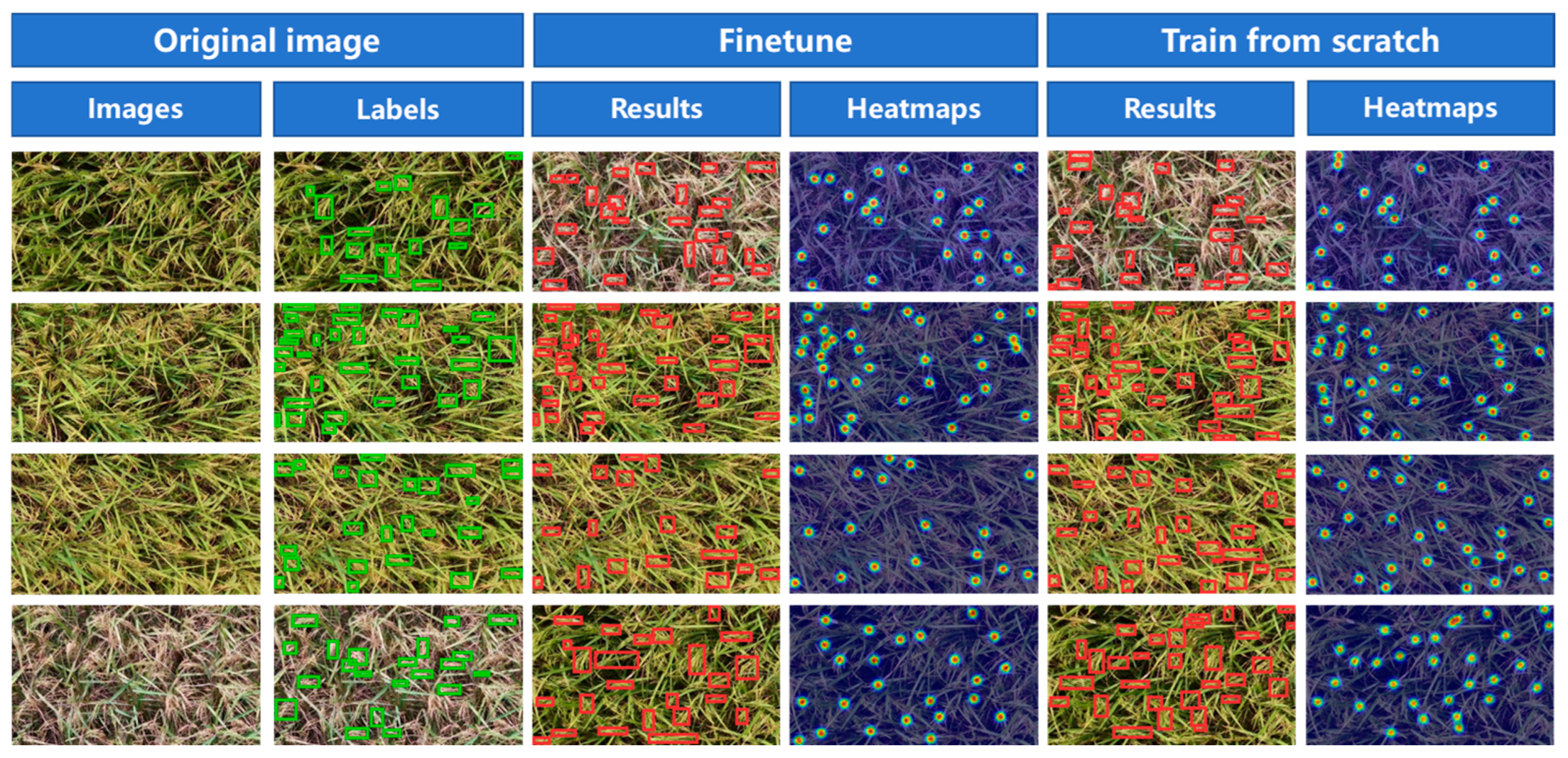
Specifically, DETR, YOLOv12, and YOLOv26 all showed higher mAP50 and lower MAE and RMSE after fine-tuning, suggesting that pretrained weights can improve detection and counting performance on the small rice dataset. However, compared with these baseline models, YOLO-DC achieved a more pronounced improvement. After fine-tuning, the mAP50 of YOLO-DC increased from 0.426 to 0.582, while MAE decreased from 5.54 to 3.82 and RMSE decreased from 7.030 to 5.018, showing larger improvements than the other models.

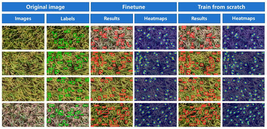
In addition, the Finetune model produces detection boxes that match the ground-truth targets more accurately, with more complete target coverage in dense regions and substantially fewer missed and false detections. Its heatmaps also show more concentrated high-response regions on the crop targets themselves, while invalid responses in background regions are effectively suppressed, indicating stronger target-focusing capability (Figure 13). In contrast, the model trained from scratch exhibits more local missed detections and box offsets, and its heatmap responses are more dispersed, reflecting weaker discrimination between foreground targets and background interference. Overall, transfer not only improves the detection and counting performance of YOLO-DC in cross-crop scenarios, but also enhances the training stability and feature transfer potential of the model.

4. Discussions and Future Work

YOLO-DC achieves a favorable balance among detection accuracy, counting error, and computational complexity. Compared with classical detectors and existing state-of-the-art methods, YOLO-DC shows clear advantages in key metrics such as mAP50, MAE, and RMSE, while maintaining relatively low parameter counts. This indicates that the proposed method not only improves crop counting accuracy but also has strong potential for lightweight deployment. Qualitative results further show that YOLO-DC provides more complete target coverage in dense regions, with substantially fewer missed detections, duplicate detections, and background-induced false positives. In addition, its response maps are more concentrated on actual crop target regions. These findings suggest that the proposed model not only improves average detection performance, but also enhances the representation, discrimination, and response stability of dense small targets in complex field environments. Nevertheless, the qualitative results also reveal several challenging failure cases. When crop targets are distributed at extremely high density, or when adjacent instances suffer from severe occlusion and strong boundary adhesion, the model may still fail to accurately distinguish individual targets, leading to missed detections, duplicate detections, or merged predictions. This indicates that, although YOLO-DC improves dense-target perception, instance-level separation under extremely crowded conditions remains a challenging problem.

From the perspective of structural design, the performance gain of YOLO-DC mainly arises from the synergy between MS-DH and LGCB-AM. Specifically, MS-DH introduces higher-resolution detection features, which effectively compensate for the loss of shallow texture, edge, and positional information caused by repeated downsampling in deep layers, thereby improving the perception of dense small objects and multi-scale targets. Meanwhile, LGCB-AM further strengthens target feature representation and suppresses background interference through attention modeling. Crop counting in agricultural scenes is not merely a general object detection problem, but is more essentially a dense small-object separation and recognition task under complex backgrounds. Therefore, relying solely on generic detection frameworks is insufficient to fully meet the demands of agricultural scenarios, and task-oriented modeling is required from the perspectives of boundary enhancement, neighborhood repulsion, fine-grained representation, and multi-scale fusion. In addition, transfer experiments further demonstrate that the edge, texture, and dense-target representations learned by YOLO-DC possess a certain degree of cross-crop transfer ability, highlighting the practical value of pretraining strategies in reducing data dependency, improving training efficiency, and enhancing model transfer ability.

Although the proposed method achieves promising results, it may still suffer from local missed detections and target confusion in extremely dense scenes with severe occlusion and highly adhered boundaries, indicating that counting methods based on detection frameworks still have limitations in instance-level fine separation. Moreover, the experiments in this study were mainly conducted on specific datasets, and the transfer ability of the model across years, regions, and crop varieties remains to be further validated. Future research may focus on the following directions: first, integrating instance segmentation, density estimation, or joint detection–segmentation frameworks to further improve target separation in extremely dense scenes; second, incorporating multi-temporal, multi-modal, and multi-scale information to enhance the adaptability of the model to dynamic changes in complex farmland environments; and third, deploying YOLO-DC on UAV-embedded edge platforms to systematically evaluate its inference speed, memory footprint, power consumption, and field operational stability, thereby promoting its practical application in smart agricultural scenarios such as crop counting, growth monitoring, and yield prediction.

5. Conclusions

This study focuses on crop detection and counting under UAV low-altitude imaging conditions, where targets are characterized by small size, dense distribution, severe mutual occlusion, and complex backgrounds, and proposes an improved crop counting network, YOLO-DC, based on deep learning. By introducing LGCB-AM and MS-DH, the proposed model effectively enhances local texture extraction, global modeling, foreground–background contrast, and boundary perception for dense small objects, thereby significantly improving detection and counting performance in complex field environments.

Experimental results demonstrate that YOLO-DC achieves strong performance, attaining a favorable balance among detection accuracy, counting error, and model efficiency. Ablation studies further verify the rationality of the proposed structural design, showing that LGCB-AM is the key contributor to the performance improvement and that its different feature extraction branches play important roles in dense-target discrimination and duplicate-count suppression. Meanwhile, a proper module insertion strategy and detection head optimization further enhance the adaptability of the network to complex agricultural scenes. Transfer experiments also indicate that YOLO-DC has good cross-crop transfer potential. Overall, YOLO-DC provides an effective solution for high-precision counting of crops such as wheat and rice under UAV platforms and also offers reliable quantitative information to support subsequent yield prediction and intelligent agricultural monitoring.

References

- Shi, Y.; Zhu, Y.; Wang, X.; Sun, X.; Ding, Y.; Cao, W.; Hu, Z. Progress and development on biological information of crop phenotype research applied to real-time variable-rate fertilization. Plant Methods 2020, 16, 11. [Google Scholar] [CrossRef] [Scilit] [PubMed]
- Saiz-Rubio, V.; Rovira-Más, F. From smart farming towards agriculture 5.0: A review on crop data management. Agronomy 2020, 10, 207. [Google Scholar] [CrossRef] [Scilit]
- Shi, S.; Ye, Y.; Xiao, R. Evaluation of food security based on remote sensing data—Taking Egypt as an example. Remote Sens. 2022, 14, 2876. [Google Scholar] [CrossRef] [Scilit]
- Bégué, A.; Arvor, D.; Bellon, B.; Betbeder, J.; de Abelleyra, D.; Ferraz, R.P.D.; Verón, S.R. Remote sensing and cropping practices: A review. Remote Sens. 2018, 10, 99. [Google Scholar] [CrossRef] [Scilit]
- Yue, W.; Gao, J.; Yang, X. Estimation of gross domestic product using multi-sensor remote sensing data: A case study in Zhejiang province, East China. Remote Sens. 2014, 6, 7260–7275. [Google Scholar] [CrossRef] [Scilit]
- Yang, L.; Mansaray, L.R.; Huang, J.; Wang, L. Optimal segmentation scale parameter, feature subset and classification algorithm for geographic object-based crop recognition using multisource satellite imagery. Remote Sens. 2019, 11, 514. [Google Scholar] [CrossRef] [Scilit]
- Carvalho, O.L.F.; de Carvalho Junior, O.A.; Albuquerque, A.O.; Bem, P.P.; Silva, C.R.; Ferreira, P.H.G.; Borges, D.L. Instance segmentation for large, multi-channel remote sensing imagery using Mask R-CNN and a mosaicking approach. Remote Sens. 2020, 13, 39. [Google Scholar] [CrossRef] [Scilit]
- Wang, X.; Yang, W.; Lv, Q.; Huang, C.; Liang, X.; Chen, G.; Duan, L. Field rice panicle detection and counting based on deep learning. Front. Plant Sci. 2022, 13, 966495. [Google Scholar] [CrossRef] [Scilit] [PubMed]
- Zang, H.; Peng, Y.; Zhou, M.; Li, G.; Zheng, G.; Shen, H. Automatic detection and counting of wheat spike based on DMseg-Count. Sci. Rep. 2024, 14, 29676. [Google Scholar] [CrossRef] [Scilit] [PubMed]
- Wen, C.; Ma, Z.; Ren, J.; Zhang, T.; Zhang, L.; Chen, H.; Guo, W. A generalized model for accurate wheat spike detection and counting in complex scenarios. Sci. Rep. 2024, 14, 24189. [Google Scholar] [CrossRef] [Scilit] [PubMed]
- Chen, Y.; Li, X.; Jia, M.; Li, J.; Hu, T.; Luo, J. Instance segmentation and number counting of grape berry images based on deep learning. Appl. Sci. 2023, 13, 6751. [Google Scholar] [CrossRef] [Scilit]
- Wang, Y.; An, J.; Shao, M.; Wu, J.; Zhou, D.; Yao, X.; Zhu, Y. A comprehensive review of proximal spectral sensing devices and diagnostic equipment for field crop growth monitoring. Precis. Agric. 2025, 26, 54. [Google Scholar] [CrossRef] [Scilit]
- Zhao, Y.; Lei, S.; Han, X.; Xu, Y.; Li, J.; Duan, Y.; Sun, S. Research on the inversion method of dust content on mining area plant canopies based on UAV-borne VNIR hyperspectral data. Drones 2025, 9, 256. [Google Scholar] [CrossRef] [Scilit]
- Zhang, H.; Wang, L.; Tian, T.; Yin, J. A Review of Unmanned Aerial Vehicle Low-Altitude Remote Sensing (UAV-LARS) Use in Agricultural Monitoring in China. Remote Sens. 2021, 13, 1221. [Google Scholar]
- Zhu, J.; Yang, G.; Feng, X.; Li, X.; Fang, H.; Zhang, J.; He, Y. Detecting wheat heads from UAV low-altitude remote sensing images using deep learning based on transformer. Remote Sens. 2022, 14, 5141. [Google Scholar] [CrossRef] [Scilit]
- Li, H.; Wang, P.; Huang, C. Comparison of deep learning methods for detecting and counting sorghum heads in UAV imagery. Remote Sens. 2022, 14, 3143. [Google Scholar] [CrossRef] [Scilit]
- Lu, C.; Nnadozie, E.; Camenzind, M.P.; Hu, Y.; Yu, K. Maize plant detection using UAV-based RGB imaging and YOLOv5. Front. Plant Sci. 2024, 14, 1274813. [Google Scholar] [CrossRef] [Scilit] [PubMed]
- Liu, L.; Yang, F.; Liu, X.; Du, Y.; Li, X.; Li, G.; Song, Z. A review of the current status and common key technologies for agricultural field robots. Comput. Electron. Agric. 2024, 227, 109630. [Google Scholar] [CrossRef] [Scilit]
- David, E.; Madec, S.; Sadeghi-Tehran, P.; Aasen, H.; Zheng, B.; Liu, S.; Kirchgessner, N.; Ishikawa, G.; Nagasawa, K.; Badhon, M.A.; et al. Global Wheat Head Detection (GWHD) Dataset: A Large and Diverse Dataset of High-Resolution RGB-Labelled Images to Develop and Benchmark Wheat Head Detection Methods. Plant Phenomics 2020, 2020, 3521852. [Google Scholar] [CrossRef] [Scilit] [PubMed]
- Admin. Drone Rice Paddy Dataset (DRPD) for UAV-Based Rice Object Detection. Explorer’s Data Nest—Deep Learning Dataset Platform. 2026. Available online: https://www.dilitanxianjia.com/20906/ (accessed on 8 June 2026).
- Tian, Y.; Ye, Q.; Doermann, D. YOLOv12: Attention-centric real-time object detectors. arXiv 2025, arXiv:2502.12524. [Google Scholar]
- Ren, S.; He, K.; Girshick, R.; Sun, J. Faster R-CNN: Towards real-time object detection with region proposal networks. Adv. Neural Inf. Process. Syst. 2015, 28, 91–99. [Google Scholar] [CrossRef] [Scilit]
- Lin, T.; Goyal, P.; Girshick, R.; He, K.; Dollár, P. Focal Loss for Dense Object Detection. In Proceedings of the IEEE International Conference on Computer Vision, Venice, Italy, 22–29 October 2017; pp. 2980–2988. [Google Scholar]
- Liu, W.; Anguelov, D.; Erhan, D.; Szegedy, C.; Reed, S.; Fu, C.-Y.; Berg, A.C. SSD: Single shot MultiBox detector. In Proceedings of the Computer Vision—ECCV 2016, Amsterdam, The Netherlands, 11–14 October 2016; pp. 21–37. [Google Scholar]
- Tian, Z.; Shen, C.; Chen, H.; He, T. FCOS: Fully convolutional one-stage object detection. In Proceedings of the IEEE/CVF International Conference on Computer Vision, Seoul, Republic of Korea, 27 October–2 November 2019; pp. 9627–9636. [Google Scholar]
- Sandler, M.; Howard, A.; Zhu, M.; Zhmoginov, A.; Chen, L.-C. MobileNetV2: Inverted residuals and linear bottlenecks. In Proceedings of the IEEE/CVF Conference on Computer Vision and Pattern Recognition, Salt Lake City, UT, USA, 18–23 June 2018; pp. 4510–4520. [Google Scholar]
- Peng, Y.; Li, H.; Wu, P.; Zhang, Y.; Sun, X.; Wu, F. D-FINE: Redefine Regression Task in DETRs as Fine-Grained Distribution Refinement. In Proceedings of the Thirteenth International Conference on Learning Representations, Singapore, 24–28 April 2025. [Google Scholar]
- Carion, N.; Massa, F.; Synnaeve, G.; Usunier, N.; Kirillov, A.; Zagoruyko, S. End-to-end object detection with transformers. In Proceedings of the Computer Vision—ECCV 2020, Glasgow, UK, 23–28 August 2020; pp. 213–229. [Google Scholar]
- Li, Y.; Wu, X.; Wang, Q.; Pei, Z.; Zhao, K.; Chen, P.; Hao, G. CSNet: A count-supervised network via multiscale MLP-Mixer for wheat ear counting. Plant Phenomics 2024, 6, 0236. [Google Scholar] [CrossRef] [Scilit] [PubMed]
- Chmcbs. HeadCount: A Semantic Segmentation Model for Counting Wheat Heads in Field Images. GitHub Repository. Available online: https://github.com/chmcbs/HeadCount (accessed on 8 June 2026).
- Wang, A.; Chen, H.; Liu, L.; Chen, K.; Lin, Z.; Han, J.; Ding, G. YOLOv10: Real-time end-to-end object detection. arXiv 2024, arXiv:2405.14458. [Google Scholar]
- Jocher, G.; Qiu, J.; Liu, M.; Lyu, S.; Akyon, F.C.; Kalfaoglu, M.E. Ultralytics YOLO26: Unified Real-Time End-to-End Vision Models. arXiv 2026, arXiv:2606.03748. [Google Scholar]
Disclaimer/Publisher’s Note: The statements, opinions and data contained in all publications are solely those of the individual author(s) and contributor(s) and not of MDPI and/or the editor(s). MDPI and/or the editor(s) disclaim responsibility for any injury to people or property resulting from any ideas, methods, instructions or products referred to in the content. |
© 2026 by the authors. Licensee MDPI, Basel, Switzerland. This article is an open access article distributed under the terms and conditions of the Creative Commons Attribution (CC BY) license.