Diffusion-Driven Relative Radiometric Normalization with Spatial–Spectral Attention Residual Network for Multi-Temporal Remote Sensing Imagery

Highlights

What are the main findings?

• A diffusion probabilistic framework decouples deterministic radiometric residuals and stochastic noise for relative radiometric normalization, overcoming limits of traditional mapping.
• The spatial–spectral attention residual network (SSARN) combines dual attention and residual learning to model cross-band spectral correlations and multi-scale spatial context of Sentinel-2 multi-temporal images.

What is the implication of the main finding?

• An SSIM-based automatic patch screening strategy selects stable training patches without manual pseudo-invariant pixel labeling, boosting model generalization over various land cover types.
• Tests on Sentinel-2 multi-temporal data show the proposed method reduces spectral distortion and delivers more stable NDVI and land cover change detection results than competing RRN methods.

Abstract

Relative radiometric normalization (RRN) is fundamental to multi-temporal remote sensing analysis; however, conventional techniques often struggle with nonlinear distortions, outlier contamination, and heterogeneous land-cover conditions. To address these challenges, we propose a diffusion-based probabilistic framework that models radiometric inconsistency as a combination of deterministic residuals and stochastic perturbations. In this framework, the forward process injects structured noise and stochastic perturbations, while the reverse process restores radiometric consistency through a dual-objective variational formulation. At the core of this framework is a spatial–spectral attention residual network (SSARN), which integrates residual learning with dual attention mechanisms to capture cross-band dependencies and multi-scale spatial context. A preprocessing stage guided by the structural similarity index (SSIM) further enhances robustness by automatically selecting stable pseudo-invariant regions for model training. Comprehensive experiments on multi-temporal Sentinel-2 datasets demonstrate that the proposed method consistently outperforms existing approaches, achieving higher accuracy and enhanced spectral fidelity. Moreover, the framework ensures greater consistency of the normalized difference vegetation index (NDVI) and preserves fine-grained textural details, underscoring its potential as a scalable and resilient solution for large-scale RRN in remote sensing applications.

1. Introduction

Radiometric rectification is an essential preprocessing step for various remote sensing applications, including spatiotemporal change detection [1,2,3], time-series image analysis [4], image mosaicking [5], drought monitoring [6], and deforestation [7]. However, radiometric inconsistencies in remotely sensed products arise from multiple factors, such as atmospheric attenuation, illumination variations, changes in sun–target–sensor geometry, and sensor instability [8,9]. These inconsistencies can lead to reflectance variations that affect the aforementioned tasks and may cause radiometric or color contrast discrepancies, as well as visible seam lines during the mosaicking of multiple remote sensing images [10]. Therefore, eliminating or mitigating these inconsistencies is crucial [11].

Radiometric normalization of remote sensing images can be categorized into absolute radiometric normalization and relative radiometric normalization (RRN) [12]. Absolute radiometric normalization aims to remove the influences of atmospheric and terrain factors and to recover absolute surface reflectance through radiometric quantization correction, typically using radiative transfer models such as 6S [13] and MODTRAN. However, the radiometric calibration process may be compromised by infrequent updates of gain and offset parameters derived from ground calibration measurements. Moreover, atmospheric correction can be affected by the spatiotemporal resolution of atmospheric parameters, potentially introducing significant accuracy errors. In some extreme cases, the unavailability of gain, offset, or aerosol optical depth parameters renders radiometric calibration and atmospheric correction problematic [11].

In contrast, RRN is more flexible in terms of timing, as it does not require field synchronous observations, thereby reducing costs and simplifying operations while maintaining acceptable accuracy. RRN can be performed using multi-temporal data acquired over the same target area. Its main advantage is the ability to normalize multi-temporal data without heavy reliance on ground synchronous observations, resulting in lower costs and repeated applicability. Unlike absolute radiometric normalization, RRN is not affected by single-date surface reflectance measurements, atmospheric parameter settings, or aerosol model choices. Furthermore, it reduces the uncertainty associated with single calibration experiments. RRN methods adjust the radiometric level of the subject image to match that of a reference image, and their appeal lies in independence from explicit physical parameters [9,14,15,16,17].

RRN constitutes a critical preprocessing step in multi-temporal remote sensing analysis. The classification of RRN methods hinges on two principal aspects: the strategy for selecting radiometric control points (which may involve manual or automated procedures) and the type of radiometric mapping function employed (which can be based on either linear or nonlinear regression paradigms). These approaches aim to mitigate radiometric variabilities arising from atmospheric, phenological, and sensor-specific factors without relying on physical parameters [3,4,18].

1.1. Manual Selection of Pseudo-Invariant Features

Among the earliest and most intuitive approaches are those relying on manual selection of pseudo-invariant features (PIFs). Techniques such as the dark set–bright set (DB) method [14] leverage domain knowledge to identify stable features for defining invariant pixels. Similarly, methods capitalizing on artificial surfaces (e.g., asphalt, rooftops) exploit spectral indices such as the infrared-to-red ratio for PIF extraction [19]. While these methods benefit from expert intuition and can yield highly accurate normalizations under controlled conditions, they suffer from inherent subjectivity, labor-intensive implementation, and limited scalability across diverse geographical regions and temporal scales [9,17].

1.2. Automated Selection of Pseudo-Invariant Features

To overcome the constraints of manual methods, numerous automated PIF selection techniques have been developed. These methods formalize the selection process through statistical or learning-based mechanisms, often conceptualized as an optimization task represented by expressions such as $R_i\times m_i$, where $R_i$ denotes feature representations derived from scattergrams or transformed domains and $m_i$ corresponds to a selection mask. For instance, principal component analysis (PCA) applied to image scattergrams enables automated radiometric control set selection (RCSS) with integrated quality assurance [20]. Similarly, the multivariate alteration detection (MAD) transformation [21,22] and its iteratively reweighted variant (IRMAD) [23] facilitate automatic identification of unchanged pixels through multispectral change vector analysis. Despite these improvements in automation, such techniques remain sensitive to distributional assumptions and threshold selections, especially under significant land-cover changes or non-Gaussian noise [24].

1.3. Regression Techniques for Radiometric Mapping

Once invariant pixels are selected, the subsequent step is to construct a radiometric mapping function. These functions are broadly categorized into linear and nonlinear models. Linear approaches, including least squares [25], orthogonal regression, and robust variants, are computationally efficient and perform reliably under linear radiometric shifts. However, they are highly susceptible to outliers and landscape changes [14]. Nonlinear techniques, such as histogram matching (HM) [26] and machine learning models like artificial neural networks (ANNs) [16] and random forests (RFs) [27], can accommodate more complex, non-Gaussian relationships. ANN architectures, in particular, can model both linear and nonlinear mappings without a priori functional assumptions, though they require significant computational resources and architectural tuning [16].

1.4. Global Versus Local Sampling Strategies

An essential methodological distinction lies in the spatial sampling strategy: global (dense) versus local (sparse) sampling. Dense RRN (DRRN) methods, including simple regression [25], haze correction [28], and global HM [26], utilize all image pixels for constructing the mapping function. While computationally efficient, these approaches are highly sensitive to land-cover changes and noise, leading to performance inconsistency when changes are substantial [7,16]. In contrast, sparse RRN (SRRN) techniques, such as PIF-based [19], DB-set [14], and histogram of oriented gradient (HOG)-based methods [29], leverage a subset of stable pixels to improve robustness against changes. Nevertheless, these methods require that the selected pixel set be both representative and sufficiently large to avoid regressive inaccuracies and overfitting [23].

1.5. Emerging Trends and Machine Learning Enhancements

Recent advances have introduced machine learning and deep learning to enhance the adaptability and accuracy of RRN. Methods incorporating random forest [26] or semantic segmentation based on HOG [29] demonstrate improved normalization outcomes by integrating feature learning and contextual information. More recently, deep learning architectures have been explored for RRN. For instance, Tang et al. [30] proposed a multi-task convolutional neural network that leverages temporal information to perform relative radiometric calibration, learning radiometric transformations across time-series images. Unsupervised domain adaptation methods, such as Cycle-Consistent Adversarial Networks (Cycle-GAN) [31], have also shown potential for aligning radiometric characteristics between unpaired multi-temporal images, reducing the need for strictly co-registered pseudo-invariant features. Despite these improvements, such methods often introduce additional complexity and hyperparameters that require careful tuning. Moreover, they may rely on idealized assumptions, such as temporal stationarity or specific statistical properties, which can limit their applicability under diverse environmental conditions [27,29].

In recent years, several advanced paradigms have emerged to further push the boundaries of RRN. To accommodate potential spatial misalignments, location-independent RRN methodologies, such as the Location-Independent RRN (LIRRN) framework, have been proposed [32]. These methods decouple radiometric mapping from strict pixel-level coordinate alignment by leveraging global feature distributions or statistical histogram matching, offering unique advantages in non-registered or poorly aligned multi-temporal imagery. Concurrently, feature-driven approaches have evolved toward tensor-based keypoint detection and switching regression frameworks [33]. Tensor-based methods preserve multi-dimensional structural topologies through higher-order tensor decompositions, whereas switching regression networks dynamically shift between discrete sub-models to capture regional land-cover variations. These emerging paradigms, while advancing the field in new directions, still face challenges in handling complex nonlinear radiometric distortions and unstructured noise, which we address in our framework.

Despite considerable progress in RRN research, prevailing methods remain constrained by several fundamental and interconnected limitations. First, the strong reliance on empirically set thresholds, as exemplified by IRMAD and histogram-based techniques, makes these methods sensitive to parameter tuning and reduces their generalizability across diverse landscapes and sensors. Second, most existing models operate under strong assumptions of linearity or global monotonicity, which are often violated in real-world scenarios characterized by complex atmospheric and phenological variations as well as atmospheric turbulence effects [34], leading to performance inconsistency under nonlinear radiometric distortions. Third, the handcrafted nature of feature selection, whether through PIFs, DB sets, or change detection strategies, fails to fully exploit the rich spectral–spatial dependencies inherent in multi-band imagery. Fourth, current approaches lack a principled mechanism for jointly modeling systematic radiometric residuals and stochastic noise, often resulting in either oversmoothed outputs or inadequate noise suppression. Finally, the inability to adaptively balance temporal change preservation with radiometric consistency limits their applicability in dynamic environments involving substantial land-cover transitions.

These challenges collectively highlight the need for a shift from heuristic and assumption-bound models toward a learnable, robust, and physically grounded framework capable of disentangling complex radiometric degradations. Such a framework should not only overcome the limitations of predefined mappings and manual parameterization but also incorporate mechanisms to explicitly model both structured radiometric biases and unstructured noise in a unified manner.

The proposed method builds on recent advances in generative modeling to address the unique challenges of multi-temporal remote sensing. By formulating radiometric differences as a combination of deterministic residuals and stochastic perturbations, we establish a principled probabilistic foundation that extends beyond conventional linear or monotonic assumptions. The core of our framework integrates the spatial–spectral attention residual network (SSARN), which incorporates dual attention mechanisms to capture cross-band interactions and multi-scale spatial context, while a diffusion-based refinement process ensures robust and accurate radiometric transfer. This formulation not only enhances adaptability across varying sensor characteristics but also provides a mathematically coherent framework for simultaneously addressing systematic errors and random noise in radiometric harmonization. Although traditional RRN methods, such as PIF, IRMAD, and CVA, do not require manually annotated training data and have achieved notable success, they still suffer from several inherent limitations. Their performance depends heavily on the predefined mapping function, and most of them rely on linear transformations, making it difficult to fully exploit the intrinsic spatial–spectral correlation characteristics in multi-band remote sensing imagery. Deep learning offers a promising alternative pathway by modeling nonlinear radiometric differences in a data-driven manner and adaptively fusing spatial and spectral information. The main contributions of this work can be summarized as follows:

(1) We propose a probabilistic framework that formulates radiometric inconsistency as a diffusion process integrating both systematic residuals and stochastic perturbations. This formulation provides a principled mathematical foundation for RRN that explicitly decouples deterministic residual correction from random noise suppression, enabling more accurate and stable radiometric consistency across diverse scenarios.

(2) We design a specialized spectral–spatial attention residual network that incorporates residual connections, group normalization, and dual attention mechanisms within a residual backbone. This configuration enhances feature representation across spectral bands and spatial scales while maintaining computational efficiency, capturing complex radiometric variations through learned attention weights.

(3) We introduce a robust preprocessing pipeline combining SSIM analysis for automatic selection of relatively unchanged image patches, ensuring high-quality training data and improved model generalization. Extensive experiments on multi-temporal Sentinel-2 datasets demonstrate that our approach consistently achieves improved performance compared with listed baselines, with lower root mean square error (RMSE) and relative mean deviation (RMD), higher peak signal-to-noise ratio (PSNR) and SSIM values, and improved vegetation index stability across varying land cover types and seasonal conditions.

2. Preliminaries

2.1. Relative Radiometric Normalization Mapping

If $\mathit{x}$ and $y$ represent the same object, differing only due to the influence of atmospheric and illumination conditions, then their relationship can be described as follows:

$$\mathit{y}=f\left(\mathit{x}\right)+\mathit{\epsilon },$$

(1)

where $f(·)$ denotes the RRN mapping function.

2.2. Diffusion Models

Diffusion models are probabilistic generative models that capture the underlying dynamics of data evolution over time [17,35]. Owing to their effective generation capability, diffusion models have gained considerable attention in various tasks, such as image generation and restoration [36]. A typical diffusion process consists of a T-step forward process and a T-step reverse process. The forward process starts with a clean image and progressively adds noise over T steps, while the reverse process operates in the opposite direction. Given a noise scheduler ${\left\{{\overline{\alpha }}_t\right\}}_{t=1}^T$ and a clean image ${\mathit{x}}_0$, adding Gaussian noise to ${\mathit{x}}_0$ iteratively over t steps yields:

$${\mathit{x}}_t=\sqrt{{\overline{\alpha }}_t}{\mathit{x}}_0+\sqrt{1-{\overline{\alpha }}_t}\mathit{ϵ},\mathit{ϵ}\sim \mathcal{N}(0,\mathit{I}).$$

(2)

A diffusion model ${\mathit{ϵ}}_{\theta }$ is trained to predict the noise as follows:

$${\mathit{ϵ}}_{\theta }({\mathit{x}}_t,t)\approx \mathit{ϵ}={\displaystyle \frac{{\mathit{x}}_t-\sqrt{{\overline{\alpha }}_t}{\mathit{x}}_0}{\sqrt{1-{\overline{\alpha }}_t}}}.$$

(3)

The reverse process starts with random noise and progressively refines the sample over T steps. Recently, numerous approaches have been proposed to accelerate the sampling process of diffusion models. A typical method is the denoising diffusion implicit model (DDIM) [37], where the forward process is modeled as non-Markovian. The model predicts the starting point as follows:

$${\widehat{\mathit{x}}}_0={\displaystyle \frac{{\mathit{x}}_t-\sqrt{1-{\overline{\alpha }}_t}{\mathit{ϵ}}_{\theta }({\mathit{x}}_t,t)}{\sqrt{{\overline{\alpha }}_t}}},$$

(4)

and then ${\mathit{x}}_{t-1}$ is sampled as:

$${\mathit{x}}_{t-1}=\sqrt{{\overline{\alpha }}_{t-1}}{\widehat{\mathit{x}}}_0+\sqrt{1-{\overline{\alpha }}_{t-1}}{\mathit{ϵ}}_{\theta }({\mathit{x}}_t,t).$$

(5)

3. Methodology

Unlike conventional RRN methods that rely on linear regression models with manually selected pseudo-invariant pixels [19,23,38], and distinct from recent deep learning approaches that do not explicitly separate systematic residuals from stochastic noise [30,31], our method addresses these limitations through a diffusion-based probabilistic framework that jointly models deterministic residuals and random perturbations. Within this framework, the radiometric difference between the subject image and the reference image is treated as a degradation process combining systematic residuals and random noise. We formulate this degradation within a diffusion-based probabilistic framework as follows.

3.1. Proposed Diffusion Framework for RRN

Let ${\mathit{x}}_0$ denote the reference image (target), and ${\mathit{x}}_{\mathrm{in}}$ the subject image (input). Define the systematic residual as ${\mathit{x}}_{\mathrm{residual}}={\mathit{x}}_{\mathrm{in}}-{\mathit{x}}_0$. The forward diffusion process gradually infuses this residual and Gaussian noise over T steps:

$${\mathit{x}}_t={\mathit{x}}_{t-1}+{\gamma }_t{\mathit{x}}_{\mathrm{residual}}+{\delta }_t{\mathit{\epsilon }}_{t-1},{\mathit{\epsilon }}_{t-1}\sim \mathcal{N}(0,\mathit{I}),$$

(6)

where ${\left\{{\gamma }_t\right\}}_{t=1}^T$ and ${\left\{{\delta }_t\right\}}_{t=1}^T$ are predefined schedules controlling the infusion of the residual and noise, respectively. Unfolding the recurrence yields:

$${\mathit{x}}_t={\mathit{x}}_0+{\overline{\gamma }}_t{\mathit{x}}_{\mathrm{residual}}+{\overline{\delta }}_t\mathit{\epsilon },$$

(7)

with ${\overline{\gamma }}_t={\sum }_{i=1}^t{\gamma }_i$, ${\overline{\delta }}_t=\sqrt{{\sum }_{i=1}^t{\delta }_i^2}$, and $\mathit{\epsilon }\sim \mathcal{N}(0,\mathit{I})$. When $t=T$, we set ${\overline{\gamma }}_T=1$, so that ${\mathit{x}}_T={\mathit{x}}_{\mathrm{in}}+{\overline{\delta }}_T\mathit{\epsilon }$.

The reverse process aims to recover ${\mathit{x}}_0$ from ${\mathit{x}}_T$ by estimating the residual and noise at each step. We employ a learnable residual network ${\mathit{x}}_{\mathrm{residual}}^{\theta }({\mathit{x}}_t,t,{\mathit{x}}_{\mathrm{in}})$ and a noise network ${\mathit{\epsilon }}_{\mathrm{noise}}^{\theta }({\mathit{x}}_t,t,{\mathit{x}}_{\mathrm{in}})$, both implemented via the proposed SSARN. The estimated clean image at step t is:

$${\mathit{x}}_0^{\theta }={\mathit{x}}_t-{\overline{\gamma }}_t{\mathit{x}}_{\mathrm{residual}}^{\theta }-{\overline{\delta }}_t{\mathit{\epsilon }}_{\mathrm{noise}}^{\theta }.$$

(8)

The reverse transition from ${\mathit{x}}_t$ to ${\mathit{x}}_{t-1}$ is defined as:

$$p_{\theta }({\mathit{x}}_{t-1}\mid {\mathit{x}}_t):=q_{\zeta }({\mathit{x}}_{t-1}\mid {\mathit{x}}_t,{\mathit{x}}_0^{\theta },{\mathit{x}}_{\mathrm{residual}}^{\theta }),$$

(9)

where $q_{\zeta }$ is a Gaussian distribution with mean:

$$\begin{array}{cc}\hfill \mathit{\mu }=& {\mathit{x}}_0^{\theta }+{\overline{\gamma }}_{t-1}{\mathit{x}}_{\mathrm{residual}}^{\theta }\hfill \\ \hfill & +\sqrt{{\overline{\delta }}_{t-1}^2-{\zeta }_t^2}{\displaystyle \frac{{\mathit{x}}_t-({\mathit{x}}_0^{\theta }+{\overline{\gamma }}_t{\mathit{x}}_{\mathrm{residual}}^{\theta })}{{\overline{\delta }}_t}},\hfill \end{array}$$

(10)

and variance ${\zeta }_t^2\mathit{I}$, with ${\zeta }_t^2=\eta {\delta }_t^2{\overline{\delta }}_{t-1}^2/{\overline{\delta }}_t^2$. The factor $\eta$ controls the stochasticity ($\eta =1$: fully random; $\eta =0$: deterministic).

The model is trained by minimizing two independent mean-squared error losses that separate the estimation of residual and noise:

$$L_{\mathrm{residual}}\left(\theta \right):=\mathbb{E}\left[{∥{\mathit{x}}_{\mathrm{residual}}-{\mathit{x}}_{\mathrm{residual}}^{\theta }({\mathit{x}}_t,t,{\mathit{x}}_{\mathrm{in}})∥}^2\right],$$

(11)

$$L_{{\epsilon }_{\mathrm{noise}}}\left(\theta \right):=\mathbb{E}\left[{∥\mathit{\epsilon }-{\mathit{\epsilon }}_{\mathrm{noise}}^{\theta }({\mathit{x}}_t,t,{\mathit{x}}_{\mathrm{in}})∥}^2\right].$$

(12)

These losses are jointly optimized to enable the reverse process to accurately reconstruct the reference image from the subject image. The overall training procedure is summarized in Algorithm 1.

Algorithm 1 Training of Diffusion-based RRN with SSARN

Require:  Training set $\left\{({\mathit{x}}_{\mathrm{in}}^i,{\mathit{x}}_0^i)\right\}$, SSIM threshold ${\tau }_s$, number of epochs N, diffusion steps T Ensure:  Trained SSARN parameters $\theta$ 1: $\mathcal{D}\leftarrow \varnothing$ 2: for each $({\mathit{x}}_{\mathrm{in}}^i,{\mathit{x}}_0^i)$ do 3:     Compute SSIM mask $M_i=\mathrm{SSIM}({\mathit{x}}_{\mathrm{in}}^i,{\mathit{x}}_0^i)\ge {\tau }_s$ 4:     Add valid pixels to $\mathcal{D}$ 5: end for 6: Initialize network parameters $\theta$ 7: for epoch $=1$ to N do 8:     for mini-batch $\left\{({\mathit{x}}_{\mathrm{in}},{\mathit{x}}_0)\right\}\subset \mathcal{D}$ do 9:         Compute residual ${\mathit{x}}_{\mathrm{residual}}={\mathit{x}}_{\mathrm{in}}-{\mathit{x}}_0$ 10:         Sample $t\sim \mathcal{U}\{1,T\}$, $\mathit{\epsilon }\sim \mathcal{N}(0,\mathit{I})$ 11:         Compute noisy state ${\mathit{x}}_t={\mathit{x}}_0+{\overline{\gamma }}_t{\mathit{x}}_{\mathrm{residual}}+{\overline{\delta }}_t\mathit{\epsilon }$▹ Use precomputed schedules 12:         Predict ${\widehat{\mathit{x}}}_{\mathrm{residual}},{\widehat{\mathit{\epsilon }}}_{\mathrm{noise}}=\mathrm{SSARN}({\mathit{x}}_t,t,{\mathit{x}}_{\mathrm{in}})$ 13:         Compute losses $L_{\mathrm{residual}}={\parallel {\widehat{\mathit{x}}}_{\mathrm{residual}}-{\mathit{x}}_{\mathrm{residual}}\parallel }^2$, $L_{\epsilon }={\parallel {\widehat{\mathit{\epsilon }}}_{\mathrm{noise}}-\mathit{\epsilon }\parallel }^2$ 14:         Update $\theta$ by minimizing $L_{\mathrm{residual}}+L_{\epsilon }$ 15:     end for 16: end for

3.2. Spatial–Spectral Attention Residual Network

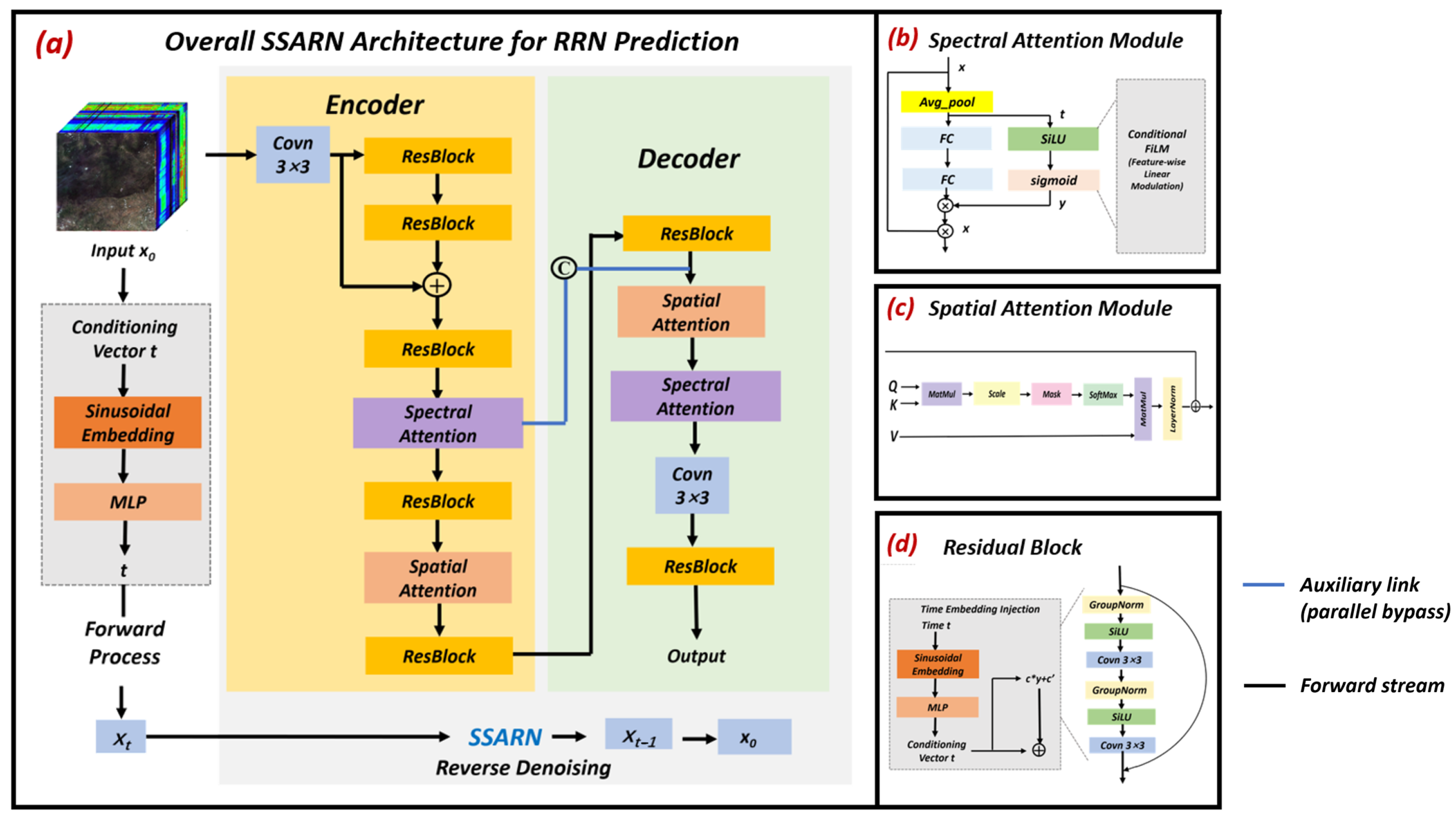
In our experiments, we employed SSARN for prediction of noise and residual features, as shown in Figure 1a. It is a deep architecture specifically designed for RRN, which builds upon an encoder–decoder backbone augmented with dual attention mechanisms and residual learning. The encoder consists of two cascaded residual blocks following an initial $3\times 3$ convolution, while the decoder incorporates dedicated spatial attention and spectral attention modules before the final convolution layer, with skip connections linking corresponding encoder and decoder stages. Each residual block (Figure 1d) integrates group normalization, a SiLU activation, and a $3\times 3$ convolution, ensuring stable gradient propagation and efficient feature transformation.

Integral to this design are the spectral attention (Figure 1b) and spatial attention (Figure 1c) modules, both placed within the decoder pathway to refine the feature representations before the output. The spectral attention module applies global average pooling followed by two fully-connected layers with a SiLU nonlinearity and a sigmoid gate, generating channel-wise scaling factors via conditional feature-wise linear modulation (FiLM) to enhance inter-band dependencies. The spatial attention module, in turn, employs layer normalization and scaled dot-product self-attention (query, key, and value projections) to model long-range spatial context, followed by group normalization, SiLU, and a $3\times 3$ convolution.

Additionally, the diffusion time step t is embedded using sinusoidal encoding and processed through a multi-layer perceptron; the resulting conditioning vector is integrated into each residual block via FiLM, enabling time-aware feature adaptation. This synergistic design enables SSARN to capture cross-band interactions, multi-scale spatial structures, and temporal dynamics, forming a backbone for inverting the complex radiometric inconsistency process within our diffusion-based RRN framework.

To provide a complete and reproducible description of the proposed model,

Table 1. Detailed architecture of the proposed diffusion model.

Component	Input	Output	Key Specs	Activation	Params ($\times {10}^3$)
Encoder	24	128	Down: 4 × 4 conv, GN	SiLU	403.6
ResBlocks	32	32	2 × (3 × 3 conv, GN)	SiLU	516.7
LinearAttn	32	32	4 heads, head_dim = 32	Softmax	86.4
SpectralAttn	32	32	FC reduction 16	ReLU + Sigmoid	7.6
Bottleneck	128	128	2 × ResBlock + 1 × Attn	SiLU/Softmax	656.2
Decoder	128	32	Up: nearest + 3 × 3 conv	SiLU	221.5
Decoder ResBlocks	192	32	2 × (3 × 3 conv, GN4)	SiLU	664.0
Decoder Attn	64	32	LinearAttn + SpectralAttn	Softmax/ReLU + Sigmoid	80.4
Output	64	12	Final ResBlock + 1 × 1 conv	SiLU	221.8
Time Embedding	t	64	Sinusoidal + 2 × FC	GELU	6.3

details the architecture of the diffusion model used in our framework. The table includes input/output dimensions, channels, key specifications (kernel size, stride, padding, group normalization, attention heads), activation functions, and per-layer parameter counts. Downsampling is implemented using $4\times 4$ strided convolutions, while upsampling employs nearest-neighbor interpolation followed by $3\times 3$ convolutions with skip connections connecting corresponding encoder and decoder stages.

4. Results

4.1. Dataset Description

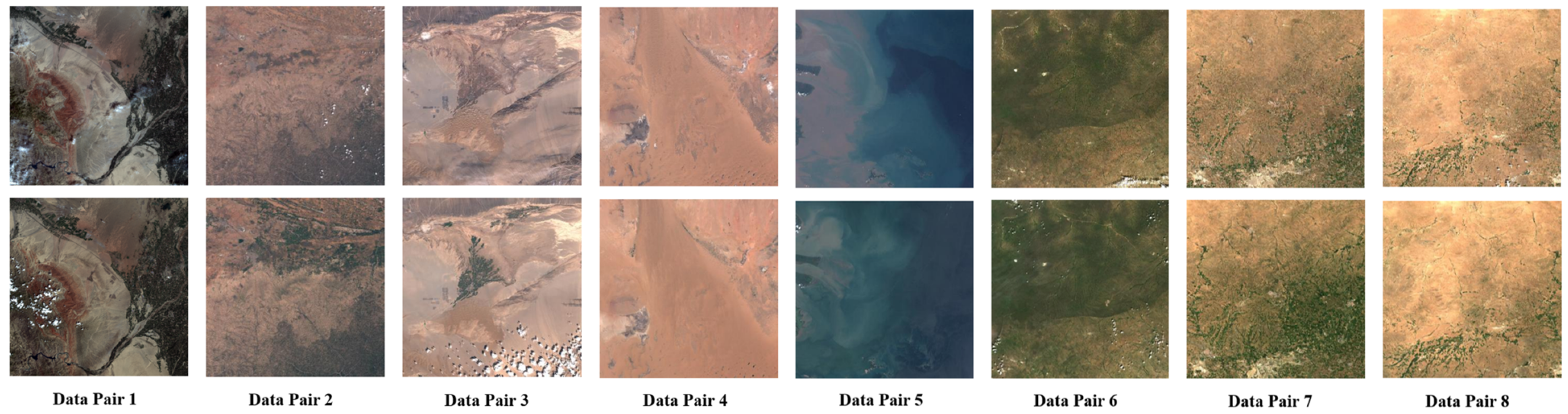
To demonstrate the effectiveness of the proposed method for RRN, eight co-registered bitemporal Sentinel-2 image pairs were collected across diverse geographical regions in China, encompassing various land cover types such as water bodies, urban areas, agricultural land, and vegetation. Each scene covers a high-resolution area of 10,944 × 10,944 or 10,980 × 10,980 pixels. All images were preprocessed to ensure strict geometric and radiometric consistency, with the cirrus 10th band discarded and spatial resampling performed via nearest-neighbor interpolation to preserve pixel values.

Data pair 1 comprises Sentinel-2B MSI Level-1C imagery from western Xinjiang, China, acquired on 20 and 30 July 2024, with minimal cloud cover and containing 13 spectral bands at 10 m, 20 m, and 60 m resolutions. The cirrus band was discarded, and lower-resolution bands were enhanced to 10 m using the Sen2Res model in SNAP. Data pair 2 features Sentinel-2B Level-1C products from Ningxia and Inner Mongolia, acquired on 5 May and 4 July 2024, showing higher cloud cover in the subject image and slight snow cover in the reference, processed similarly. Data pair 3 includes Sentinel-2B Level-1C scenes from western Xinjiang from 2 November 2023 and 29 July 2024, with moderate cloud coverage and negligible snow, undergoing identical resolution enhancement. Data pair 4 covers the Inner Mongolia–Gansu border with images from 21 October 2023 and 17 July 2024, notable for being entirely cloud-free and having minimal snow cover, processed to uniform 10 m resolution. Data pair 5 is from Shanghai with acquisitions on 17 October 2023 and 2 August 2024, showing very low cloud in the subject image and higher cloud cover in the reference, with no snow and standard preprocessing. Data pair 6 consists of Sentinel-2 Level-2A products from the Mongolia–northern China border, with a Sentinel-2A subject image from 29 July 2023, and a Sentinel-2B reference from 7 August 2024, featuring low cloud and nearly absent snow, with all bands resampled to 10 m. Data pair 7 involves Sentinel-2A Level-2A imagery from the China–Mongolia border from 19 July 2023 and 23 July 2024, with extremely low cloud and snow cover, processed to 10 m resolution. Data pair 8 contains Sentinel-2A Level-2A products from the Inner Mongolia–Hebei border, acquired on 19 July 2023 and 23 July 2024, also with very low cloud and snow percentages, and all coarser bands sharpened to 10 m using Sen2Res. All datasets are georeferenced in geographic coordinates, and the cirrus band was consistently excluded during analysis.

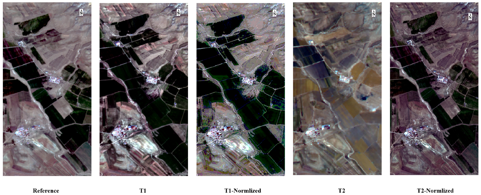
The dataset collected for the proposed method, along with the corresponding pseudo-color composite of the normalized subject images, is shown in Figure 2. In our experimental setup, data pairs 1 to 7 from Figure 2 were used for training, while data pair 8 was reserved for testing. All training data were processed by cropping into non-overlapping 256 × 256 image patches. The patches selected for the training set were chosen based on SSIM computed between each corresponding pair of image patches from the reference and subject images. A threshold of 0.75 was empirically selected for the SSIM value to identify suitable patch pairs for training. This specific criterion was determined to balance the size of the training sample against the precision of the radiometric correspondence: a higher threshold would retain fewer but nearly identical patches, potentially limiting the diversity and volume of the training set, whereas a lower threshold would include more variable pairs at the risk of introducing undesired spectral changes or misregistration artifacts. The 0.75 threshold ensures a large number of high-quality samples that exhibit strong radiometric consistency while still accommodating natural variability and minor misalignments, thereby supporting both sufficient data volume for effective learning and high radiometric normalization accuracy.

4.2. Implementation Details

To ensure reproducibility, we provide detailed training hyperparameters and computational specifications. All experiments were conducted on a workstation equipped with an Intel Xeon Gold 6248R CPU and a single NVIDIA GeForce RTX 4090 GPU with 24 GB GDDR6X memory. The proposed model was trained for 200 epochs with a batch size of 8 using the AdamW optimizer and a cosine annealing learning rate schedule with an initial learning rate of $1\times {10}^{-4}$, resulting in a total training time of approximately 18.6 h. During inference, the reverse diffusion process employs 50 DDIM steps with $\eta =0$, yielding an inference time of approximately 252 s per full Sentinel-2 scene. The total number of trainable parameters in the SSARN architecture is approximately 2.86 million for a single U-Net. The forward diffusion process employed $T=1000$ steps. All experiments were conducted using the PyTorch v1.11.0 framework.

4.3. Accuracy Estimation of RRN

For RRN quality evaluation, we utilize the following metrics.

First, the RRN methods were assessed in terms of the average RMSE:

$$\mathrm{RMSE}=\sqrt{{\mathbb{E}}_{({\mathit{I}}_{\mathrm{subject}},{\mathit{I}}_{\mathrm{ref}})}{\left(f\left({\mathit{I}}_{\mathrm{subject}}\right)-{\mathit{I}}_{\mathrm{ref}}\right)}^2},$$

(13)

where ${\mathit{I}}_{\mathrm{subject}}$ denotes the subject image and ${\mathit{I}}_{\mathrm{ref}}$ represents the reference image. A smaller RMSE indicates better radiometric normalization performance.

Second, the average RMD was adopted on the test data as follows:

$$\mathrm{RMD}={\displaystyle \frac{\left|{\mathit{I}}_{\mathrm{ref}}-{\mathit{I}}_{\mathrm{subject}}\right|}{{\mathit{I}}_{\mathrm{ref}}}}\times 100\%.$$

(14)

The acceptable normalized image quality derived from RRN is characterized by a low RMD.

Two additional quantitative metrics, SSIM and PSNR, were employed to assess the quality of the normalized images generated by the proposed method relative to the reference images. These metrics were computed for each spectral band on the test dataset. Higher SSIM and PSNR values indicate more accurate and faithful radiometric normalization results.

4.4. Comparison of RRN Methods

To demonstrate the capability of the proposed RRN method, we compared it with the following prevalent approaches: (1) HM: histogram matching [26]; (2) MM: minimum–maximum [14]; (3) SR: simple regression [25]; (4) PIF: pseudo-invariant feature approach [19]; (5) PCA: principal component analysis [20]; (6) UCLR: normalization using linear regression with unchanged pixels [24]; (7) ANN: normalization based on artificial neural networks with unchanged pixels [16]; (8) HOG-based: normalization based on HOG features as the RCSS [29]; (9) IRMAD: iteratively reweighted MAD transformation-based normalization [23]; (10) CVA: change vector analysis [38]; (11) OC2: orthogonal correction-2nd order [39]; (12) MT-CNN [30]; and (13) Cycle-GAN [31].

Table 2. RMSE comparison of different RRN methods across spectral bands.

Method	Band 1	Band 2	Band 3	Band 4	Band 5	Band 6	Band 7	Band 8	Band 9	Band 10	Band 11	Band 12	Avg.
RAW	1973.5922	2143.5861	2626.8572	3116.3429	3487.4966	3943.2049	4150.8891	4127.0721	4310.9394	4304.5037	5017.5457	4509.8773	3642.6589
ANN	1235.4580	1083.0787	672.2350	480.1129	295.8145	182.1166	188.7641	189.6909	186.0588	187.1030	201.7528	206.1736	425.6966
HOG-based	208.3290	218.1694	225.8385	325.3709	282.5254	327.8775	379.9567	415.0992	380.1070	403.2242	370.4483	444.5597	331.7921
HM	220.5806	225.5771	230.3846	302.8480	276.7692	320.4917	355.3461	364.9964	353.3994	415.4834	330.8421	384.2616	315.0817
CVA	197.6505	210.9302	224.3305	284.5532	254.2546	268.4061	324.1718	352.7540	317.9225	355.2781	318.7232	375.6691	286.0537
UCLR	194.6038	211.5061	223.2839	327.3444	281.8206	326.9985	378.3109	396.5890	380.4927	398.4955	370.9137	446.5753	328.0779
PCA	245.1519	241.2161	236.4648	324.7925	281.9941	330.4940	398.0564	462.7854	398.1681	431.8359	358.6080	444.2814	346.1540
IRMAD	180.3736	194.1512	205.9464	290.4983	257.5516	289.3782	325.0913	332.0433	323.9188	356.2060	324.3594	386.5761	288.8412
MM	2478.6417	581.8557	939.6838	855.3248	323.8498	650.1660	538.3864	492.3578	719.8956	4118.3042	367.3701	439.2312	1042.0889
PIF	188.8754	207.4550	221.3233	326.3140	280.7606	328.0458	379.2744	393.3346	381.5297	400.0947	370.5328	445.1828	326.8936
OC2	801.2293	1267.9049	1565.7424	1772.6479	1193.0046	1119.1353	1111.2556	2286.3532	1081.7974	949.9311	1175.9898	1221.6838	1295.5563
SR	240.2839	278.6465	335.8015	505.6251	467.6585	406.2256	464.6096	464.3254	461.7148	476.1591	588.0876	669.5896	446.5606
MT-CNN	186.7466	200.3213	211.9094	292.5082	262.8789	299.8093	336.8945	344.7744	335.5453	369.1013	326.8910	381.9799	295.7801
Cycle-GAN	201.0704	215.7261	228.2572	314.9476	283.0583	322.8493	362.8489	371.3151	361.3424	397.4517	352.1084	410.0706	318.4211
Ours	179.5921	192.6467	203.7909	281.3017	252.8077	288.3232	323.9876	331.5656	322.6901	354.9605	314.3674	367.4940	284.4606

and

Table 3. RMD comparison of different RRN methods across spectral bands.

Method	Band 1	Band 2	Band 3	Band 4	Band 5	Band 6	Band 7	Band 8	Band 9	Band 10	Band 11	Band 12	Avg.
RAW	33.25	36.11	44.26	52.50	58.76	66.43	69.93	69.53	72.63	72.52	84.54	75.98	61.37
ANN	20.81	18.25	11.33	8.09	4.98	3.07	3.18	3.20	3.13	3.15	3.40	3.47	7.17
HOG-based	5.52	5.43	4.90	6.87	5.10	4.95	5.58	6.58	5.37	5.22	4.77	6.85	5.59
HM	3.65	4.37	4.35	5.98	4.57	4.32	4.64	4.82	4.43	4.20	4.11	5.77	4.60
CVA	3.38	4.10	4.13	5.83	4.38	4.19	4.52	4.68	4.33	4.07	4.10	5.79	4.46
UCLR	4.39	5.02	4.80	6.91	5.07	4.96	5.57	5.98	5.39	5.07	4.78	6.87	5.40
PCA	8.37	7.05	5.45	7.02	5.11	5.82	7.12	9.09	6.88	7.02	4.80	7.11	6.74
IRMAD	3.39	4.18	4.20	6.06	4.48	4.20	4.55	4.70	4.36	4.09	4.25	6.09	4.54
MM	41.76	9.80	15.83	14.41	5.46	10.95	9.07	8.30	12.13	69.38	6.19	7.40	17.56
PIF	3.96	4.79	4.73	6.88	5.05	4.97	5.55	5.82	5.37	5.07	4.77	6.85	5.32
OC2	13.50	21.36	26.38	29.87	20.10	18.86	18.72	38.52	18.23	16.00	19.81	20.58	21.83
SR	7.18	8.40	9.19	12.15	10.14	7.15	7.31	7.32	6.92	6.67	8.83	11.13	8.53
MT-CNN	3.54	4.32	4.35	6.15	4.61	4.39	4.73	4.89	4.53	4.24	4.31	6.10	4.68
Cycle-GAN	4.33	5.28	5.31	7.52	5.64	5.36	5.77	5.98	5.53	5.18	5.26	7.45	5.72
Ours	3.39	4.11	4.14	5.76	4.37	4.20	4.48	4.65	4.29	4.01	4.00	5.61	4.42

indicate that the proposed diffusion-based RRN method consistently achieves improved performance across all 12 spectral bands, yielding the lowest average RMSE of 284.4606 and the lowest average RMD of 4.42 among all evaluated methods. This signifies minimal spectral distortion and high radiometric consistency in the normalized outputs. The proposed method slightly surpasses the strong reference method IRMAD, which attained an RMSE of 288.8412 and an RMD of 4.54, and which itself considerably outperforms most conventional approaches. Among the other methods, CVA also demonstrates competitive performance, with an RMSE of 286.0537 and an RMD of 4.46, confirming the effectiveness of change vector analysis for identifying invariant pixels. MT-CNN and Cycle-GAN achieve average RMSE values of 295.78 and 318.42, and average RMD values of 4.68 and 5.72, respectively. ANN exhibits a contradictory behavior: while its average RMD of 7.17 is relatively low, suggesting generally acceptable spectral preservation, it yields the second-highest RMSE of 425.6966, indicating high sensitivity to outliers and possible instability in bands with strong radiometric differences. HOG-based, UCLR, and PIF form a cluster of mid-tier performers, with average RMSE values around 326 to 332 and RMD values around 5.3 to 5.6, implying that while the selection of stable features or pixels is beneficial, the use of uniform coefficients or linear models limits their precision. HM performs commendably among global methods, with an RMSE of 315.0817 and an RMD of 4.60, even outperforming some sparse RRN (SRRN) techniques, though its inability to separate changed and unchanged regions constrains further improvement. PCA correction introduces noticeable spectral distortion, as evidenced by its highest RMD value of 6.74 among SRRN methods, likely due to its sensitivity to variations in principal components. In contrast, MM and SR perform poorly, with MM being particularly unsuitable due to its extreme amplification of errors in certain bands, such as the RMSE of 4118.30 in Band 10, a consequence of relying on global min-max stretching. OC2 results, with an RMSE of 1295.5563 and an RMD of 21.83, resemble those of the raw images.

The quantitative comparison of the evaluated RRN methods is further summarized in

Table 4. Average PSNR (dB) and SSIM values across all 12 spectral bands for all evaluated methods.

Method	Avg. PSNR (dB)	Avg. SSIM
ANN	25.83	0.4767
HOG-based	13.96	0.8673
HM	35.01	0.9693
CVA	35.59	0.9025
UCLR	34.63	0.9053
PCA	34.25	0.9246
IRMAD	35.83	0.9038
MM	27.27	0.9092
PIF	34.79	0.9044
OC2	22.89	0.6041
SR	31.96	0.9275
MT-CNN	36.09	0.9725
Cycle-GAN	35.68	0.9689
Ours	38.63	0.9866

, which reports the average PSNR and average SSIM across all 12 spectral bands. The proposed method achieves the highest average PSNR of 38.63 dB and the highest average SSIM of 0.9866, demonstrating improved signal fidelity and structural preservation among all compared approaches. Among the other methods, MT-CNN yields the second-best performance with an average PSNR of 36.09 dB and an average SSIM of 0.9725, followed closely by Cycle-GAN and HM. IRMAD delivers a competitive average PSNR of 35.83 dB but a lower average SSIM of 0.9038, indicating that while its radiometric correction is effective in terms of intensity error, it preserves structural information less reliably. CVA, UCLR, PCA, and PIF exhibit moderate average PSNR values ranging from 34.25 dB to 35.59 dB and average SSIM values between 0.9025 and 0.9246, suggesting generally acceptable but not outstanding normalization quality. In contrast, the HOG-based method shows a notably low average PSNR of 13.96 dB yet a relatively high average SSIM of 0.8673, implying that it retains structural patterns but fails to correct radiometric magnitudes accurately. ANN and OC2 perform poorly, with average PSNR values of 25.83 dB and 22.89 dB, and average SSIM of 0.4767 and 0.6041, respectively, indicating severe degradation in both signal accuracy and structural fidelity. MM and SR achieve intermediate results, with SR outperforming MM.

To further validate the statistical properties and stability of the proposed method against the IRMAD and CVA approaches, given the modest numerical gaps observed in the average metrics, we supplemented our evaluation with paired-sample t-tests, variance analysis, and 95% confidence intervals based on the per-band results reported in Table 2 and Table 3. The paired t-test results indicate that the proposed method yields p-values of 0.023 for RMSE and 0.018 for RMD when compared with IRMAD, and p-values of 0.031 for RMSE and 0.025 for RMD when compared with CVA. In terms of numerical dispersion, the proposed method produces an RMSE variance of 12.47 and an RMD variance of 0.081, compared with 28.62 and 0.153 for IRMAD, and 25.19 and 0.137 for CVA. The 95% confidence interval for the average RMSE of our method ranges from 281.21 to 287.71, and that for RMD ranges from 4.38 to 4.46. These intervals compare with those of IRMAD, which range from 285.36 to 292.32 for RMSE and from 4.49 to 4.59 for RMD, and with those of CVA, which range from 283.14 to 288.97 for RMSE and from 4.42 to 4.50 for RMD. These results suggest that the proposed method offers improved precision and lower variability across spectral bands relative to the two baseline methods under the current experimental settings.

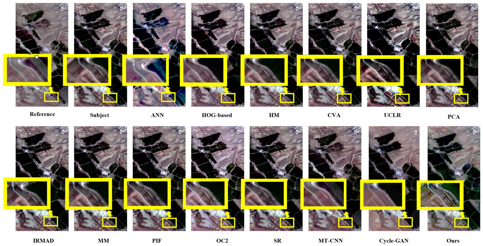
To evaluate the RRN performance qualitatively, visual interpretation was conducted among the reference image, the original subject image, and the normalized results generated by various methods, as provided in Figure 3. The subject image displays evident radiometric discrepancies compared to the reference, including reduced brightness and inconsistent contrast across different land cover types, such as vegetation, bare soil, roads, and water bodies–likely due to seasonal and acquisition interval effects.

Most normalization methods improve radiometric consistency to some extent. The proposed method produces a normalized image that is visually most similar to the reference, with harmonized contrast and natural texture representation across all land covers. This outcome aligns with its top quantitative performance, reinforcing its effectiveness. Methods such as IRMAD and CVA also yield visually convincing results with minor residual variations, consistent with their strong quantitative rankings. MT-CNN and Cycle-GAN produce visually plausible results but exhibit slight spectral distortions or residual artifacts in heterogeneous regions, reflecting their moderate quantitative performance.

HOG-based, UCLR, and PIF show partial correction but still exhibit localized over- or under-adjustment, correlating with their intermediate quantitative scores. The result of ANN preserves general spectral properties in some areas but introduces visible artifacts in regions with high radiometric variance, supporting its previously noted sensitivity to outliers.

Methods like PCA and HM exhibit limited radiometric alignment. PCA introduces noticeable spectral distortion, while HM improves global contrast but fails to address local inconsistencies. The poorest-performing methods, such as MM and OC2, show minimal improvement or even further inconsistency, appearing almost identical to the original subject image in certain bands, which corresponds to their low quantitative performance.

The improved visual quality achieved by the proposed method can be attributed to its diffusion-based framework, which systematically reverses radiometric inconsistency through iterative refinement. The embedded spectral and spatial attention mechanisms in the SSARN network facilitate effective integration of multi-scale and cross-band features, while the explicit modeling of both residual and noise components ensures accurate correction of complex radiometric perturbations. These characteristics enable the proposed method to produce visually coherent and radiometrically stable results, even in challenging scenarios involving diverse land covers and varied atmospheric conditions.

Although the proposed method introduces higher computational complexity than conventional RRN approaches, it provides improved capability for modeling nonlinear radiometric discrepancies and exploiting spatial–spectral contextual information, leading to improved normalization performance in heterogeneous multi-temporal scenes.

It is also worth clarifying the relationship between our method and other recent deep learning-based RRN frameworks. WEGLA-NormGAN [40] represents a significant advance in deep learning-based RRN, but it is specifically designed for seamless large-scale mosaicking of remote sensing images, where the core objective is to produce visually smooth and radiometrically consistent image products free of seam lines. Its evaluation framework is therefore centered on image-level perceptual and structural similarity metrics, such as SSIM, PSNR, SAM, LPIPS, and GS, which measure the visual fidelity of the generated outputs. In contrast, our work is explicitly oriented toward serving downstream analysis tasks, particularly change detection and NDVI consistency assessment. The fundamental goal of our method is to use RRN as a preprocessing step to improve the accuracy of subsequent quantitative applications. Accordingly, our evaluation goes beyond traditional image quality indicators by designing specific experiments that verify the practical benefits of normalization for downstream tasks, as demonstrated in Section 5.2 and Section 5.3. These differences in application orientation mean that the success criteria of the two methods are inherently different, making a direct numerical comparison less meaningful. Furthermore, while comprehensive toolboxes such as SpectralMatch [41] emphasize engineering implementation and broad applicability, our work differs fundamentally in its methodological philosophy by adopting a generative diffusion framework to model the stochastic nature of radiometric degradation.

5. Discussion

5.1. Ablation Study

To verify the effectiveness of each core module in the proposed model and to elucidate the contributions of the spectral attention module (SAM), the spatial attention module (SPA), and the diffusion model architecture to the relative radiometric normalization performance, a series of ablation experiments was designed. These experiments were conducted by selectively removing or replacing individual core modules to establish ablation control groups. All experiments were performed on the same Sentinel-2 test dataset, with quantitative evaluation based on RMSE and RMD. The ablation results are summarized in

Table 5. Ablation study of key components: RMSE and RMD comparison.

Metric	Without SSIM	Without SAM	Without SPA	Without Diffusion	Ours
Average RMSE	385.1956	301.2482	308.7543	295.3111	284.4606
Average RMD	6.01	4.96	5.07	4.82	4.42

.

The ablation experiments quantitatively evaluate the contribution of each key component to model performance. First, the effectiveness of the SSIM-based selection mechanism is validated. Compared to the strategy without SSIM selection, adopting SSIM selection reduces RMSE by 100.73 and RMD by 1.59. This significant reduction in error metrics demonstrates that training on a clean dataset composed of pixels with high structural similarity enables the diffusion model to learn a more accurate and robust radiometric transformation function, thereby confirming the necessity of the SSIM-based sample selection strategy. The removal of SAM indicates that SAM enhances spectral discriminability; it also suggests that relying solely on spatial attention is insufficient to fully capture cross-band dependencies, highlighting the importance of synergizing spectral and spatial attention. The removal of SPA shows that SPA models long-range spatial dependencies among pixels, improving the consistency between local texture and the global structure of the image, thus complementing SAM. Replacing the diffusion model with a standard U-Net yields error metrics that are inferior to the baseline, indicating that the probabilistic modeling capability of the diffusion model mitigates local artifacts and radiometric overcorrection commonly observed in conventional U-Net architectures, achieving a better balance between radiometric correction accuracy and spatial detail preservation.

5.2. Vegetation Change Detection with RRN

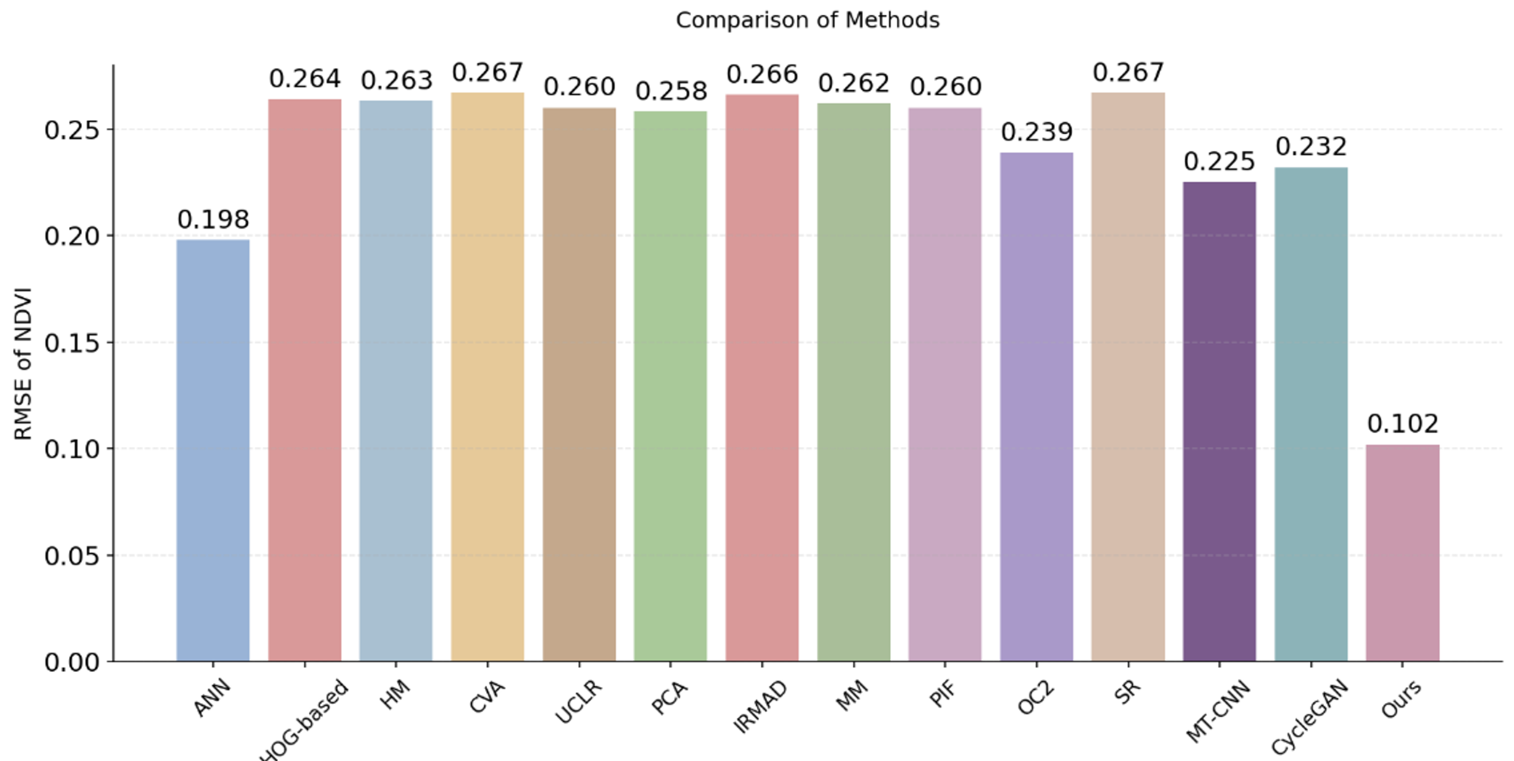
To quantitatively evaluate the performance of different radiometric normalization methods in terms of vegetation index consistency, the RMSE of NDVI was calculated between the normalized images and the reference image. As summarized in Figure 4, the proposed method achieves a lower NDVI RMSE of 0.102, outperforming all other compared methods by a significant margin.

Among the other approaches, ANN demonstrates the second-best performance with an NDVI RMSE of 0.198, though it remains considerably higher than that of the proposed method. Techniques such as HOG-based, HM, CVA, UCLR, PCA, IRMAD, MM, PIF, and SR yield results in a narrow range between approximately 0.26 and 0.27, indicating limited effectiveness in recovering accurate NDVI values. OC2 performs slightly better than this group with an RMSE of 0.239, yet it still falls short of the proposed method’s accuracy. MT-CNN and Cycle-GAN achieve moderate NDVI RMSE values of 0.225 and 0.232, respectively, which are lower than those of the aforementioned group but still higher than that of the proposed method.

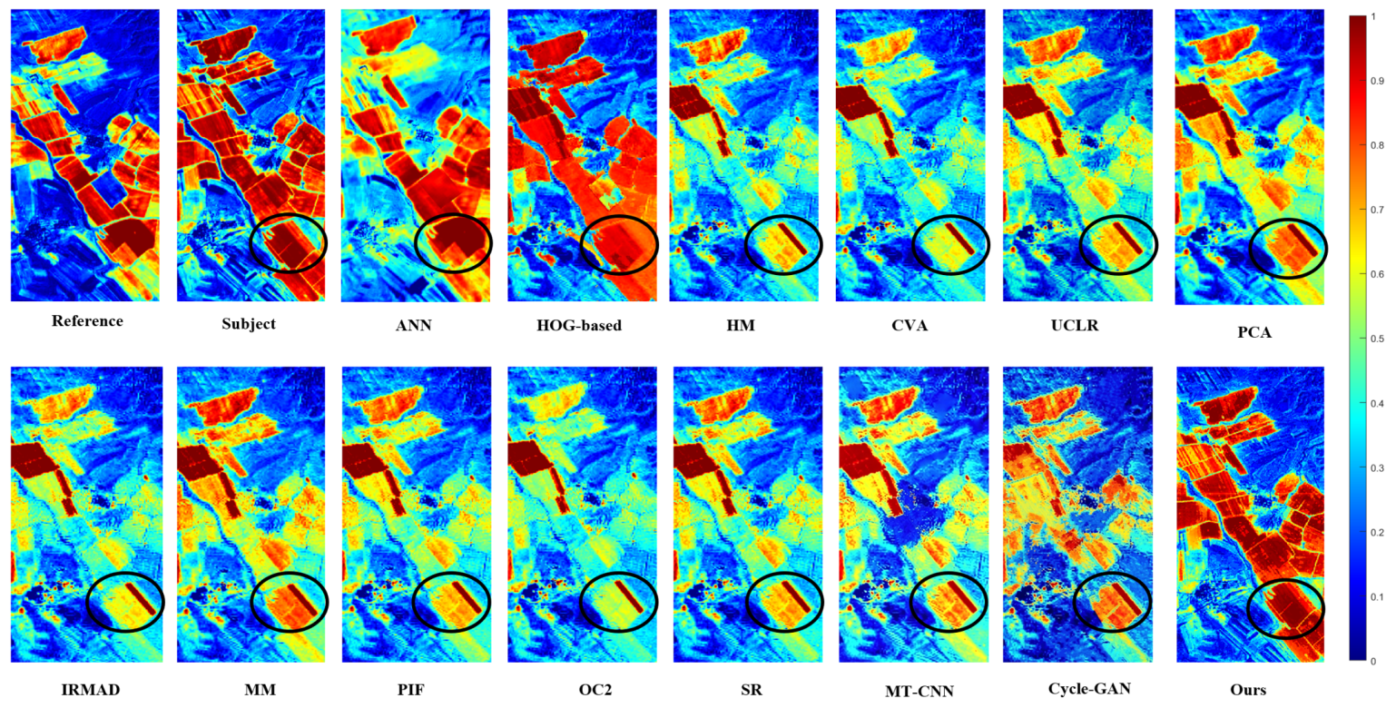
The visual comparison of NDVI images, as partially illustrated in Figure 5, supports these quantitative findings. The NDVI result generated by the proposed method exhibits markedly improved consistency with the reference NDVI in terms of spatial distribution and numerical range. Vegetated areas are better differentiated from non-vegetated surfaces, and edge details are more coherent with the reference. In contrast, most other methods produce NDVI images with visible residual radiometric discrepancies, spurious variations in homogeneous regions, and reduced contrast between land cover types. Although ANN offers relatively acceptable visual results in certain areas, it still introduces noticeable artifacts in regions with high ecological variability. The NDVI results obtained by MT-CNN and Cycle-GAN show some improvement over traditional methods but still exhibit local spectral inconsistencies and reduced contrast in heterogeneous landscapes, consistent with their intermediate quantitative RMSE values.

The improved performance of the proposed method can be attributed to its ability to model complex, nonlinear radiometric relationships between the subject and reference images through a deep diffusion-based process. By explicitly minimizing both radiometric residuals and spectral distortion in a learned feature space, the method preserves the spectral characteristics necessary for accurate vegetation index computation. In comparison, methods relying on linear adjustments (e.g., UCLR, SR), hand-crafted features (e.g., HOG-based), or global statistics (e.g., HM, PCA) fail to adequately compensate for localized and non-uniform radiometric deviations, particularly in vegetated regions where subtle spectral differences are critical.

These results underscore the capability of the proposed normalization method not only in improving pixel-level radiometric accuracy but also in enhancing the quality of derived products such as NDVI. This is especially important for applications requiring precise vegetation monitoring, change detection, and time-series analysis. The method’s robustness across different spectral domains confirms its potential for operational use in multi-temporal remote sensing studies.

5.3. Change Detection with RRN

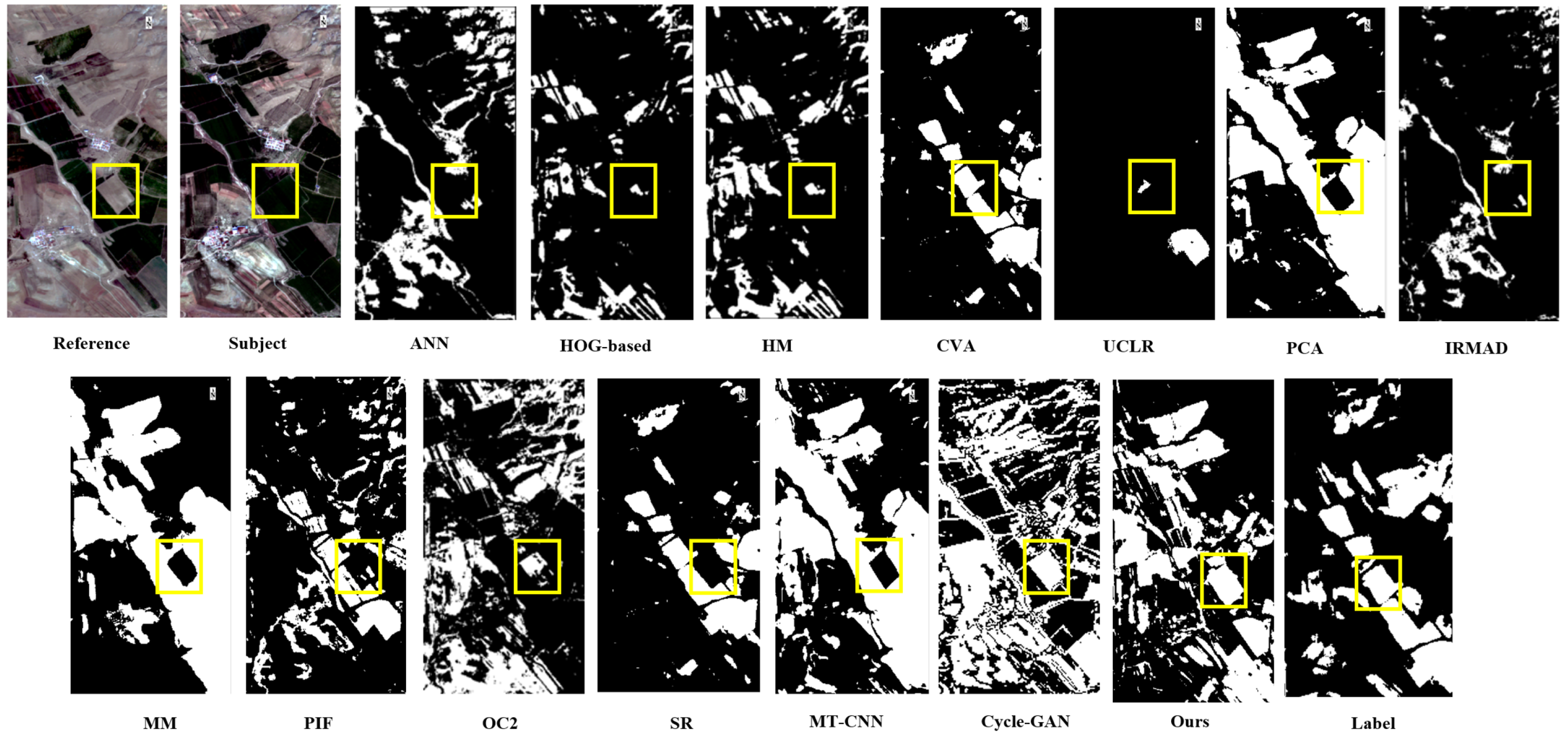
A visual analysis of the change detection results derived from the normalized images with various radiometric normalization methods, as shown in Figure 6, reveals notable differences in the ability of each approach to support reliable land-cover change identification. The proposed method produces a change map that is visually closest to the ideal reference–subject difference, demonstrating a strong capacity to suppress radiometric inconsistencies while retaining meaningful changes.

In the result generated by the proposed method, changes such as new construction, vegetation loss, or water body shrinkage are clearly delineated with minimal spurious noise in stable regions. This indicates that the method reduces radiometric biases between the subject and reference images. In comparison, methods such as IRMAD and CVA also perform reasonably well, but close inspection shows residual high-frequency discrepancies in homogeneous areas such as croplands or bare soil, suggesting incomplete normalization.

Other techniques, including HM, UCLR, and PCA, yield change maps with noticeable residuals, particularly in bright or shadowed regions, leading to both false alarms and missed detections. For instance, HM preserves global contrast but fails to adjust local variations, causing over-detection in urban edges. PCA introduces spectral distortion that manifests as speckle-like artifacts across the change map.

The result of ANN exhibits fragmented error patterns, likely due to model sensitivity to outliers and radiometric extremes. Similarly, the HOG-based method shows inconsistent performance across land cover types, with visible errors around textural boundaries. Methods relying on global adjustments without selective sample use, such as SR and MM, perform poorly, with MM particularly amplifying errors in high dynamic range bands, resulting in large false change regions.

MT-CNN produces change maps with moderate accuracy, achieving a precision of 0.68 and a recall of 0.61, which are lower than those of the proposed method but higher than many traditional approaches. However, its change boundaries are often less precise, and some genuine changes are missed. Cycle-GAN yields a precision of 0.51 and a recall of 0.47, indicating frequent false alarms and omission errors. Its change maps exhibit noticeable artifacts and inconsistent detection across different land cover types, consistent with its lower quantitative metrics.

The improvement observed with the proposed method can be attributed to its ability to explicitly model both radiometric residuals and structured noise in a unified deep learning framework, leveraging iterative diffusion-based refinement. By incorporating spatial and spectral attention mechanisms, the method achieves enhanced invariance to illumination, phenology, and sensor-specific effects, which are critical requirements for producing clean and reliable change maps.

We annotated change masks, which were then reviewed by two experts. Final labels required agreement of the experts. To quantitatively validate the improvement in change detection reliability, we compared the change detection binary maps obtained from each normalization method against a manually labeled ground truth mask. The quantitative metrics, including precision, recall, F1-score, and kappa coefficient, are summarized in

Table 6. Quantitative evaluation of change detection performance using different RRN methods.

Method	Precision	Recall	F1-Score	Kappa
ANN	0.42	0.38	0.40	0.35
HOG-based	0.57	0.53	0.55	0.49
HM	0.70	0.67	0.69	0.61
CVA	0.65	0.61	0.63	0.55
UCLR	0.43	0.33	0.37	0.35
PCA	0.70	0.66	0.68	0.62
IRMAD	0.69	0.62	0.65	0.60
MM	0.55	0.50	0.52	0.47
PIF	0.77	0.75	0.76	0.69
OC2	0.59	0.54	0.56	0.50
SR	0.66	0.62	0.64	0.58
MT-CNN	0.68	0.61	0.64	0.54
Cycle-GAN	0.51	0.47	0.49	0.43
Ours	0.76	0.79	0.78	0.73

.

As shown in Table 6, the proposed method achieves the highest F1-score and Kappa coefficient, outperforming all other compared methods. Notably, although PIF achieves comparable precision, its recall is lower than that of our method, resulting in an F1-score of 0.76 versus our 0.78. This demonstrates that the proposed method not only reduces false positives but also captures genuine changes more comprehensively.

5.4. Multi-Temporal Image Sequence Evaluation

To further verify the effectiveness of the proposed method in long-term time-series remote sensing applications, we conducted experiments on a multi-temporal image sequence consisting of three temporally consecutive Sentinel-2 images acquired from July 2023 to July 2025 over the same study area. All images were normalized to a common reference date using the proposed method. To visually validate the preservation of genuine temporal change while eliminating radiometric inconsistencies, we present the normalized results in Figure 7. The figure shows the false-color composites of the reference image, the subject image before normalization, the normalized result produced by the proposed method, and the corresponding difference image between the reference and the normalized result. It can be observed that the proposed method removes radiometric discrepancies while preserving realistic land-cover changes.

These results confirm that the proposed diffusion-based framework removes radiometric discrepancies while preserving temporal dynamics, indicating its suitability for large-scale time-series remote sensing applications.

It is worth noting how our proposed generative diffusion paradigm conceptually diverges from recent keypoint-based and location-independent frameworks such as LIRRN [32]. Frameworks like LIRRN are inherently designed to bypass geometric registration errors, making them ideal for unaligned image pairs. However, for strictly co-registered multi-temporal datasets like the Sentinel-2 pairs utilized in our experiments, discarding spatial coordinate constraints would cause a substantial loss of localized context. Our SSARN architecture explicitly exploits these precise spatial alignments through dual-attention mechanisms. Furthermore, while tensor-based and switching regression frameworks [33] model radiometric variations via discrete multi-model switching or structured sparse keypoint alignment, they often exhibit limited tolerance to non-structured multi-temporal noise. Our framework resolves this by treating the normalization process as a continuous reverse diffusion procedure, thereby elegantly separating complex nonlinear atmospheric degradation from invariant ground reflectance in a seamless and end-to-end differentiable manner.

5.5. Computational Efficiency Analysis

To evaluate the practical deployability of the proposed method, we analyzed its computational cost in terms of training time and inference time, comparing it against representative fast linear methods (IRMAD, CVA) and a global method (HM). All experiments were conducted on a single NVIDIA GTX 4090 GPU. The proposed diffusion model was trained for 200 epochs with a batch size of 8, using the training set described in Section 4.1. The reverse sampling process employed 50 DDIM steps ($\eta =0$) as a practical trade-off between reconstruction quality and speed.

Table 7. Computational cost comparison of different RRN methods.

Method	Training Time (Hours)	Inference Time (Seconds per Scene)	Sampling Steps (If Any)
IRMAD	—	12	—
CVA	—	18	—
HM	—	8	—
ANN	2.5	35	—
Ours	18.6	252	50

Note: “—” indicates not applicable or not available.

reports the total training time (where applicable) and the average inference time per full Sentinel-2 scene. IRMAD, CVA, and HM require no training, while ANN and the proposed method require offline training. As shown, the proposed method incurs higher computational cost than linear baselines but remains within a practical range for batch processing.

The inference time of the proposed method is approximately 21× slower than IRMAD, which is primarily attributable to the iterative denoising process inherent to diffusion models. However, two important factors should be considered. First, the training phase is performed only once for a given sensor configuration and can be reused for all subsequent scenes. Second, the proposed method achieves consistently improved radiometric accuracy compared to IRMAD and outperforms faster methods in NDVI consistency and change detection reliability. Our diffusion-based method involves iterative denoising, leading to a notable rise in inference time. Even so, for application scenarios where normalization accuracy is the core priority, this trade-off between computational overhead and improved performance is reasonable.

5.6. Sensitivity Analysis of SSIM Preselection Threshold

The proposed method employs an SSIM-based sample selection strategy to filter training patches, with a threshold ${\tau }_s$ determining the minimum structural similarity between a subject-reference patch pair for inclusion in the training set. In the main experiments, ${\tau }_s$ was empirically set to 0.75. To rigorously justify this choice and to assess the sensitivity of model performance to this hyperparameter, we conducted a systematic sensitivity analysis.

Specifically, we varied ${\tau }_s$ from 0.5 to 0.9 in increments of 0.1. For each threshold, we re-trained the entire diffusion-based RRN model from scratch using the same training data and evaluated the normalized results on the same test scene using the average RMSE across all 12 spectral bands. The results are summarized in

Table 8. Sensitivity of average RMSE to different SSIM thresholds ${\tau }_s$.

${\mathit{\tau }}_{\mathit{s}}$	0.50	0.60	0.70	0.75	0.80	0.90
Average RMSE	312.4588	298.7179	289.6342	284.4606	285.1272	291.3854

.

At the intermediate threshold of ${\tau }_s=0.75$, the model achieves the lowest RMSE of 284.4606. This threshold retains a sufficiently large and diverse set of training patches while filtering out most patches with genuine changes or severe misregistration. It strikes an optimal balance between sample quality, sample quantity, and sample diversity. The performance degradation is relatively mild when ${\tau }_s$ varies between 0.7 and 0.8, indicating that the proposed method is reasonably robust to the exact threshold choice within this range. However, thresholds above 0.8 are not recommended, as the sharp decline in sample size undermines model generalization.

6. Conclusions

This study presents a diffusion-based probabilistic framework for relative radiometric normalization of multi-temporal remote sensing imagery. The key improvement lies in reformulating RRN as the reversal of learned radiometric inconsistencies, which enables robust separation of complex radiometric residuals and stochastic noise. The integration of a dedicated spatial–spectral attention residual network further enhances the model’s ability to capture cross-band dependencies and multi-scale spatial features, resulting in highly precise normalization. A preprocessing stage based on SSIM is employed to automatically select stable pseudo-invariant regions for training, enhancing model accuracy and generalization. Extensive quantitative and qualitative evaluations on Sentinel-2 datasets demonstrate that the proposed method consistently outperforms listed approaches, including IRMAD, CVA, and neural network-based techniques such as ANN. Improved performance is confirmed across multiple metrics, including RMSE, RMD, PSNR, and SSIM, highlighting its capacity to achieve radiometric fidelity and structural similarity relative to reference images. Critically, the method also improves practical downstream applications, yielding more accurate NDVI estimations and cleaner and more reliable change detection maps by minimizing false alarms while preserving genuine land-cover variations. These results establish diffusion models as an effective paradigm for RRN, providing a generalized, high-performance solution that reduces reliance on hand-crafted features and heuristic thresholds. Future work will explore extending the model to handle more complex and extreme radiometric variations while further enhancing its robustness and computational efficiency for operational deployment.

References

1. Hui, Y.; Xu, B.; Huang, H.; Yu, Q.; Gong, P. Modelling spatial-temporal change of Poyang Lake using multitemporal Landsat imagery. Int. J. Remote Sens. 2008, 29, 5767–5784. [Google Scholar]
2. Bovolo, F.; Bruzzone, L. A theoretical framework for unsupervised change detection based on change vector analysis in the polar domain. IEEE Trans. Geosci. Remote Sens. 2006, 45, 218–236. [Google Scholar] [CrossRef]
3. Ghosh, A.; Mishra, N.S.; Ghosh, S. Fuzzy clustering algorithms for unsupervised change detection in remote sensing images. Inf. Sci. 2011, 181, 699–715. [Google Scholar] [CrossRef]
4. Vicente-Serrano, S.M.; Perez-Cabello, F.; Lasanta, T. Assessment of radiometric correction techniques in analyzing vegetation variability and change using time series of Landsat images. Remote Sens. Environ. 2008, 112, 3916–3934. [Google Scholar] [CrossRef]
5. Zhang, Y.; Yu, L.; Sun, M.; Zhu, X. A mixed radiometric normalization method for mosaicking of high-resolution satellite imagery. IEEE Trans. Geosci. Remote Sens. 2017, 55, 2972–2984. [Google Scholar] [CrossRef]
6. Yan, N.; Wu, B.; Boken, V.K.; Chang, S.; Yang, L. A drought monitoring operational system for China using satellite data: Design and evaluation. Geomat. Nat. Hazards Risk 2016, 7, 264–277. [Google Scholar]
7. Schultz, M.; Verbesselt, J.; Avitabile, V.; Souza, C.; Herold, M. Error sources in deforestation detection using BFAST monitor on Landsat time series across three tropical sites. IEEE J. Sel. Top. Appl. Earth Obs. Remote Sens. 2015, 9, 3667–3679. [Google Scholar] [CrossRef]
8. Teillet, P. Image correction for radiometric effects in remote sensing. Int. J. Remote Sens. 1986, 7, 1637–1651. [Google Scholar] [CrossRef]
9. Yang, X.; Lo, C. Relative radiometric normalization performance for change detection from multi-date satellite images. Photogramm. Eng. Remote Sens. 2000, 66, 967–980. [Google Scholar]
10. Liu, S.; Lian, J.; Zhan, X.; Liu, C.; Tian, Y.; Duan, H. Automatically eliminating seam lines with Poisson editing in complex relative radiometric normalization mosaicking scenarios. arXiv 2021, arXiv:2106.07441. [Google Scholar]
11. Liu, S.; Wang, L.; Lian, J.; Liu, C.; Zhan, X.; Liu, J.; Wang, T.; Geng, D.; Duan, H.; Zou, S. Auto robust relative radiometric normalization via latent change noise modeling. IEEE Trans. Geosci. Remote Sens. 2024, 62, 5405415. [Google Scholar] [CrossRef]
12. Chen, Y.; Sun, K.; Li, D.; Bai, T.; Li, W. Improved relative radiometric normalization method of remote sensing images for change detection. J. Appl. Remote Sens. 2018, 12, 045018. [Google Scholar] [CrossRef]
13. Vermote, E.F.; Tanre, D.; Deuze, J.L.; Herman, M.; Morcette, J.J. Second simulation of the satellite signal in the solar spectrum, 6S: An overview. IEEE Trans. Geosci. Remote Sens. 1997, 35, 675–686. [Google Scholar] [CrossRef]
14. Hall, F.G.; Strebel, D.E.; Nickeson, J.E.; Goetz, S.J. Radiometric rectification: Toward a common radiometric response among multidate, multisensor images. Remote Sens. Environ. 1991, 35, 11–27. [Google Scholar] [CrossRef]
15. Bao, N.; Lechner, A.M.; Fletcher, A.; Mellor, A.; Mulligan, D.; Bai, Z. Comparison of relative radiometric normalization methods using pseudo-invariant features for change detection studies in rural and urban landscapes. J. Appl. Remote Sens. 2012, 6, 063578. [Google Scholar] [CrossRef]
16. Sadeghi, V.; Ebadi, H.; Ahmadi, F.F. A new model for automatic normalization of multitemporal satellite images using artificial neural network and mathematical methods. Appl. Math. Model. 2013, 37, 6437–6445. [Google Scholar] [CrossRef]
17. Zhou, H.; Liu, S.; He, J.; Wen, Q.; Song, L.; Ma, Y. A new model for the automatic relative radiometric normalization of multiple images with pseudo-invariant features. Int. J. Remote Sens. 2016, 37, 4554–4573. [Google Scholar] [CrossRef]
18. Tu, Y.H.; Phinn, S.; Johansen, K.; Robson, A. Assessing radiometric correction approaches for multi-spectral UAS imagery for horticultural applications. Remote Sens. 2018, 10, 1684. [Google Scholar] [CrossRef]
19. Salvaggio, C. Radiometric scene normalization utilizing statistically invariant features. In Proceedings of the Workshop on Atmospheric Correction of Landsat Imagery, Torrance, CA, USA, 29 June–1 July 1993; pp. 155–159. [Google Scholar]
20. Du, Y.; Teillet, P.M.; Cihlar, J. Radiometric normalization of multitemporal high-resolution satellite images with quality control for land cover change detection. Remote Sens. Environ. 2002, 82, 123–134. [Google Scholar] [CrossRef]
21. Canty, M.J.; Nielsen, A.A.; Schmidt, M. Automatic radiometric normalization of multitemporal satellite imagery. Remote Sens. Environ. 2004, 91, 441–451. [Google Scholar] [CrossRef]
22. Nielsen, A.A.; Conradsen, K.; Simpson, J.J. Multivariate alteration detection (MAD) and MAF postprocessing in multispectral, bitemporal image data: New approaches to change detection studies. Remote Sens. Environ. 1998, 64, 1–19. [Google Scholar] [CrossRef]
23. Canty, M.J.; Nielsen, A.A. Automatic radiometric normalization of multitemporal satellite imagery with the iteratively re-weighted MAD transformation. Remote Sens. Environ. 2008, 112, 1025–1036. [Google Scholar] [CrossRef]
24. Ya’allah, S.M.; Saradjian, M.R. Automatic normalization of satellite images using unchanged pixels within urban areas. Inf. Fusion 2005, 6, 235–241. [Google Scholar] [CrossRef]
25. Jensen, J.R. Urban/suburban land use analysis. In Manual of Remote Sensing, 2nd ed.; Wiley: Falls Church, VA, USA, 1983; pp. 1571–1666. [Google Scholar]
26. Richards, J.A.; Richards, J. Remote Sensing Digital Image Analysis, 3rd ed.; Springer: Berlin, Germany, 1999. [Google Scholar]
27. Seo, D.; Kim, Y.; Eo, Y.; Park, W.; Park, H. Generation of radiometric, phenological normalized image based on random forest regression for change detection. Remote Sens. 2017, 9, 1163. [Google Scholar] [CrossRef]
28. Chavez, P.S. An improved dark-object subtraction technique for atmospheric scattering correction of multispectral data. Remote Sens. Environ. 1988, 24, 459–479. [Google Scholar] [CrossRef]
29. He, H.; Liu, X.; Shen, Y. Relative radiometric correction of high-resolution remote sensing images based on feature category. Clust. Comput. 2018, 22, 7933–7941. [Google Scholar] [CrossRef]
30. Tang, L.; Zhao, X.; Hu, X.; Luo, C.; Lin, M. A Multi-Task Convolutional Neural Network Relative Radiometric Calibration Based on Temporal Information. Remote Sens. 2024, 16, 3346. [Google Scholar] [CrossRef]
31. Zhu, J.Y.; Park, T.; Isola, P.; Efros, A.A. Unpaired Image-to-Image Translation Using Cycle-Consistent Adversarial Networks. In Proceedings of the IEEE International Conference on Computer Vision (ICCV), Venice, Italy, 22–29 October 2017; pp. 2223–2232. [Google Scholar]
32. Moghimi, A.; Sadeghi, V.; Mohsenifar, A.; Celik, T.; Mohammadzadeh, A. LIRRN: Location-Independent Relative Radiometric Normalization of Bitemporal Remote-Sensing Images. Sensors 2024, 24, 2272. [Google Scholar] [PubMed]
33. Moghimi, A.; Celik, T.; Mohammadzadeh, A. Tensor-based keypoint detection and switching regression model for relative radiometric normalization of bitemporal multispectral images. Int. J. Remote Sens. 2022, 43, 3927–3956. [Google Scholar] [CrossRef]
34. Mao, H.M.; Ding, Z.Y.; Yang, Y.Y.; Jiang, S.Q.; Peng, J.T.; Cao, N.; Hu, L.F.; Cao, Z.L. Effect of atmospheric turbulence on imaging quality of high-resolution remote sensing satellites. Chin. Opt. 2024, 17, 167–177. [Google Scholar] [CrossRef]
35. Ho, J.; Jain, A.; Abbeel, P. Denoising diffusion probabilistic models. Adv. Neural Inf. Process. Syst. 2020, 33, 6840–6851. [Google Scholar]
36. Song, Y.; Ermon, S. Generative modeling by estimating gradients of the data distribution. Adv. Neural Inf. Process. Syst. 2019, 32, 1–11. [Google Scholar]
37. Song, J.; Meng, C.; Ermon, S. Denoising Diffusion Implicit Models. arXiv 2020, arXiv:2010.02502. [Google Scholar]
38. Malila, W.A. Change vector analysis: An approach for detecting forest changes with Landsat. In Proceedings of the Sixth Annual Symposium held by Purdue University’s Laboratory for Applications of Remote Sensing (LARS), West Lafayette, IN, USA, 3–6 June 1980; p. 385. [Google Scholar]
39. Yuan, D.; Elvidge, J.C. Comparison of relative radiometric normalization techniques. ISPRS J. Photogramm. Remote Sens. 1996, 51, 117–126. [Google Scholar] [CrossRef]
40. Gan, W.; Feng, Y.; Miao, J.; Li, X.; Shen, H. WEGLA-NormGAN: Wavelet-enhanced Cycle-GAN with global-local attention for radiometric normalization of remote sensing images. ISPRS J. Photogramm. Remote Sens. 2026, 233, 39–54. [Google Scholar]
41. SpectralMatch. Available online: https://github.com/ (accessed on 19 June 2026).
Figure 1. Overview of the spatial–spectral attention residual network.
Remotesensing 18 02156 g001
Figure 2. Visualization of eight data pairs (data pair 1 to data pair 8). For each data pair, the top image represents the reference acquisition, while the bottom image represents the subject acquisition from a different time point. All images are presented as standardized false-color composite thumbnails.
Remotesensing 18 02156 g002
Figure 3. Visual comparison of different RRN methods. The figure shows the reference image, the subject image, and the results obtained by ANN, HOG-based, HM, CVA, UCLR, PCA, IRMAD, MM, PIF, OC2, SR, MT-CNN, Cycle-GAN, and the proposed method. Yellow rectangles highlight representative regions of interest where radiometric discrepancies are most pronounced, facilitating visual comparison across different methods.
Remotesensing 18 02156 g003
Figure 4. RMSE of NDVI between the subject image after radiometric normalization using different methods and the reference image.
Remotesensing 18 02156 g004
Figure 5. Comparison of NDVI results derived from different RRN methods. From top to bottom, left to right: reference image, subject image, and results from ANN, HOG-based, HM, CVA, UCLR, PCA, IRMAD, MM, PIF, OC2, SR, MT-CNN, Cycle-GAN, and the proposed method. Black circles highlight local comparisons.
Remotesensing 18 02156 g005
Figure 6. Visual comparison of change detection results between reference and subject images using different radiometric normalization methods. From left to right, top to bottom: reference image, subject image, ANN, HOG-based, HM, CVA, UCLR, PCA, IRMAD, MM, PIF, OC2, SR, MT-CNN, Cycle-GAN, the proposed method, and label. Yellow boxes highlight local comparisons.
Remotesensing 18 02156 g006
Figure 7. Multi-temporal normalization results.
Remotesensing 18 02156 g007