The Topological Detection of Spatially Proximate Emitters in Spaceborne-Radio-Environment Maps: An ImprovedPersistent-Homology Approach

Highlights

What are the main findings?

• We introduced synthetic-aperture passive-interferometric-imaging technology to construct a spaceborne-REM-simulation dataset. A PH-AC unsupervised-detection framework is proposed, and this achieves high-precision, low-complexity adaptive emitter detection.
• By tracking merging events via persistent homology and extracting multidimensional topological features, the issue of separating “conjoined” structures (caused by the superposition of intensity fields from spatially proximate emitters) in REMs is effectively resolved.

What are the implications of the main findings?

• PH-AC, without requiring any annotated data and with low computational cost, achieves detection accuracy that surpasses traditional image-processing methods and is comparable to the deep learning YOLOv13 method. This provides a lightweight solution for spaceborne real-time detection that does not rely on large-scale annotated datasets.
• REM-based emitter detection is fundamental to electromagnetic situational awareness, but traditional methods struggle to separate emitters when spatially proximate sources form “conjoined” structures due to intensity-field superposition. PH-AC addresses this issue by tracking connected component-merging events via persistent homology, enabling reliable emitter detection in densely deployed scenarios.

Abstract

Existing radio environment map(REM)-based emitter-detection methods suffer from high false positives and missed detections in blurred or conjoined structures, or require large annotated datasets and heavy computation. We propose an unsupervised method, persistent homology with agglomerative clustering (PH-AC), based on an improved persistent-homology algorithm. A simulated spaceborne-REM dataset is constructed via synthetic-aperture passive interferometric imaging, covering isolated, adjacent-pair, and complex-emitter distributions. Persistent homology tracks the birth, death, and merging of zero-dimensional connected components as the intensity threshold varies. To address missed detections for spatially proximate emitters, multidimensional topological features are constructed via feature-contribution analysis. Agglomerative clustering with Ward linkage then adaptively separates emitters from noise without supervision. Experimental results show that PH-AC achieves a perfect F1 score of 1.000 in isolated scenarios; for adjacent emitters, it improves F1 by 15.7% over the best image-processing method and stays within 4% of supervised deep learning methods, while requiring no annotations. In complex environments, it attains an F1 of 0.937, outperforming all compared methods. Its computational complexity is only $2.25\times {10}^6$ FLOPs, three orders lower than YOLO-based detectors. This work offers a lightweight, annotation-free topological paradigm for spaceborne-REM-emitter detection.

1. Introduction

With the explosive growth of global electromagnetic devices and wireless communication technologies, the electromagnetic environment has become increasingly complex, and the generation of wide-area radio-environment maps (REMs) has emerged as a significant topic in the domain of spatial situational awareness [1,2]. At present, the construction of spectrum maps primarily relies on terrestrial platforms, which are constrained by line-of-sight limitations and, thus, incapable of achieving extensive coverage [3,4,5]. Existing spaceborne sensing approaches—whether optical imaging [6,7,8,9], synthetic-aperture radar [10], or conventional electronic reconnaissance methods [11,12,13]—generally suffer from low efficiency in terms of acquiring the overall situational picture of emitter clusters, an inherent trade-off between field of view and resolution, and insufficient real-time imaging capabilities [14,15]. To overcome these bottlenecks, this study draws upon synthetic-aperture passive-interferometric-imaging techniques from the field of natural-thermal-radiation remote sensing and adapts them to the context of anthropogenic electromagnetic-situation generation [16]. By employing multiple antenna elements to passively receive signals from ground stations, the spatial-distribution image of emitters is directly reconstructed through interferometric processing, thereby achieving wide-field imaging capability while maintaining high resolution. Furthermore, the update cycle of spectrum maps is compressed from the hour/day level associated with conventional “point sampling plus post-processing” to the second level, thus offering a novel technical pathway for the rapid generation of spaceborne wide-area REMs [17,18]. To enable the rapid generation of spaceborne wide-area electromagnetic-spectrum maps, it is important to develop REM-based applications. The foundation of such applications is emitter detection, and how to efficiently detect emitters from REMs becomes the key to transforming imaging capability into actionable situational awareness. Compared with traditional passive-localization methods that rely on single-point direction finding or parameter association, spaceborne REMs possess distinct advantages such as intuitive spatial-distribution representation, the capacity for synchronous observation of large-scale regions, and the elimination of complex signal-deinterleaving procedures. Consequently, the development of emitter-detection techniques based on spaceborne REMs holds considerable significance for enhancing real-time early-warning and target-interpretation capabilities in complex electromagnetic environments [19].

Existing emitter-detection methods based on REMs are primarily classified into image-processing techniques and object-detection techniques, both of which continue to face numerous challenges. Image-processing techniques extract emitters by enhancing high-frequency details or segmenting high-intensity regions: wavelet transform highlights high-frequency features through multi-scale decomposition [20], yet in scenarios with blurred boundaries, detail coefficients are difficult to separate from background noise. Xu Shoulong et al. proposed a morphological filtering method that employs Top-hat transformation to extract bright targets [21,22,23,24], but this method relies on predefined structuring elements and tends to merge multiple targets when adjacent emitters become connected; Hakan Işıker et al. introduced Otsu multilevel thresholding for image segmentation based on global grayscale statistics [25,26,27,28,29], yet thresholds are difficult to determine accurately when the contrast between emitters and background is low; and Wang Xuegang et al. modeled the spectrum map as a high-dimensional tensor and employed a maximum-value method for emitter detection after reconstruction [30], which is primarily suited to prominent “hot spots” and inapplicable to multi-emitter scenarios. Statistical detection methods, represented by the global RX detector, calculate anomaly scores via Mahalanobis distance [31,32,33,34,35] but assume that the background follows a multivariate Gaussian distribution. In complex non-stationary environments, background statistical characteristics are difficult to describe with a single distribution, and the superposition of intensity fields from adjacent emitters alters local statistical properties, leading to increased false alarm rates or missed detections. Object-detection techniques, exemplified by the YOLO series, achieve end-to-end detection through convolutional neural networks [36,37,38,39,40,41]. These methods depend on large-scale, precisely annotated radio-environment-map data, the acquisition cost of which is prohibitively high; meanwhile, their computational cost is substantial, rendering them inadequate for meeting the real-time requirements of spaceborne platforms. Moreover, the Non-Maximum Suppression mechanism inherent to such methods struggles to accurately estimate the number of emitters in scenarios involving adjacent emitters. The FreqFusion module proposed by Chen et al. addresses intra-class inconsistency and boundary ambiguity in feature fusion through adaptive low-pass and high-pass filtering as well as offset correction [42,43,44,45]. The YOLOv13_FreqFusion model compared in this study incorporates this module, yet it remains supervised and computationally expensive. In recent years, researchers have explored improvement strategies from various perspectives. With respect to lightweight detection, Mobilenet-SSD reduces computational load through depthwise separable convolution [46,47,48,49], yet its detection accuracy for small targets and adjacent emitters is limited. To enhance the discrimination of proximate targets, some studies have introduced Transformer architectures; for instance, DETR replaces NMS with a global attention mechanism [50,51,52,53], but its slow convergence and high computational overhead make it unsuitable for spaceborne real-time constraints.

To address the aforementioned issues, we propose an emitter-detection method for REMs based on improved persistent homology (PH-AC), which fully exploits the topological structural information of the intensity field within the radio-environment map. This method does not rely on manual annotation. By tracking the birth, death, and merging events of connected components as the intensity threshold varies, topological features that reflect emitter stability are extracted, and agglomerative clustering is employed to achieve adaptive separation of emitters and noise. The principal contributions of this paper are as follows:

(1)

Based on the rapid-generation technique for spaceborne REMs using synthetic-aperture technology proposed in prior research [16], a simulated dataset of spaceborne REMs encompassing three emitter-distribution patterns is constructed, thereby providing a data benchmark for the study of emitter-detection methods.

(2)

The persistent-homology method, originally developed for topological-data analysis, is innovatively applied to the domain of emitter detection in REMs. An emitter-feature-extraction module based on persistent homology is proposed, addressing the difficulty that conventional methods encounter in distinguishing adjacent emitters.

(3)

Hierarchical agglomerative clustering with Ward linkage is employed for unsupervised classification on the basis of the extracted multidimensional topological features. The clustering results are automatically mapped to emitter and noise categories according to the physical interpretation of persistence, thereby overcoming the challenge of adaptive discrimination that traditional threshold-dependent methods fail to address.

The remainder of this paper is structured as follows: Section 2 introduces the construction process of the simulated dataset of spaceborne REMs; Section 3 elaborates on the proposed method, covering data preprocessing, feature extraction, and classification modules; Section 4 validates the detection performance and computational efficiency of the proposed method through comparative experiments and ablation studies; and Section 5 concludes the paper and discusses future research directions.

2. Data Simulation

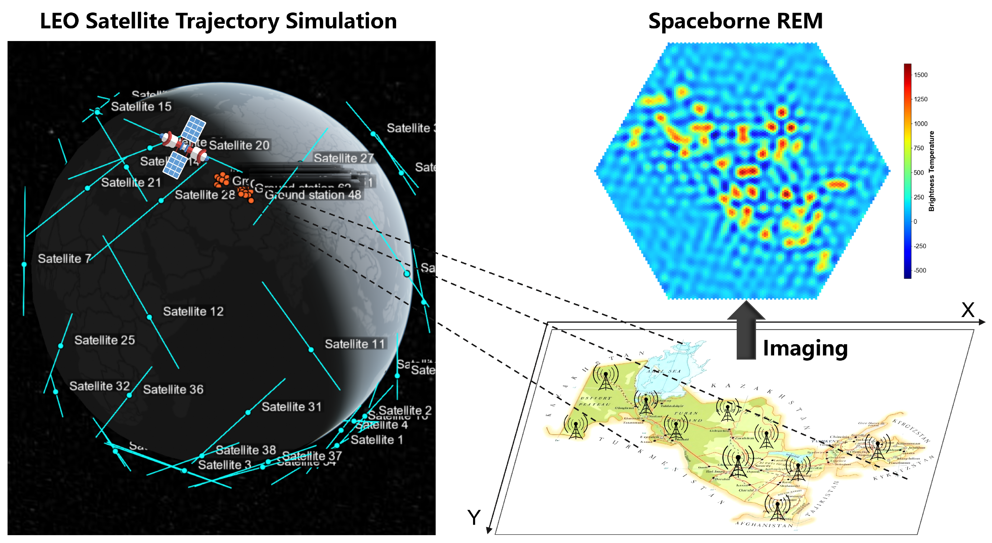
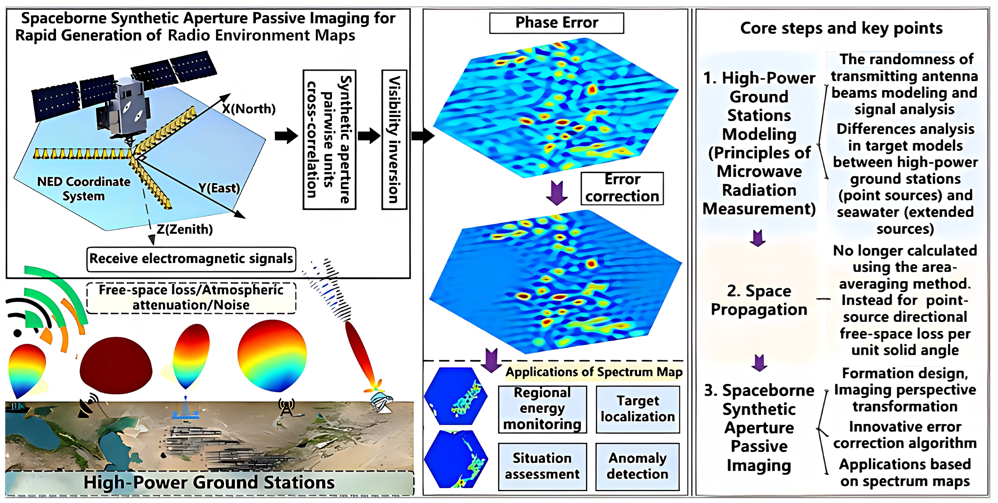
In our prior research, the synthetic-aperture passive-interferometric-imaging technique, traditionally employed for natural-thermal-radiation imaging of ground features and seawater, was adapted to the domain of electromagnetic-spectrum sensing. Through interdisciplinary intersection and technological integration, a theoretical model encompassing “emitter signal transmission—free-space propagation—spaceborne synthetic-aperture passive imaging” was established, and a method for the rapid generation of spaceborne wide-area REMs was proposed [16]. The framework is illustrated in Figure 1. To validate the effectiveness of the emitter-detection method, we construct a simulated dataset of spaceborne REMs based on this approach. Utilizing the MATLAB Satellite Toolbox, a low-Earth-orbit-satellite scenario is established with the Uzbekistan region as the simulation scene, a center frequency of 1.5 GHz (L-band), and three distinct emitter-distribution patterns.

2.1. Principles of Spaceborne-Radio-Environment-Map Simulation

We temporarily adopted the amplitude-modulation (AM) signal as the research subject. It is assumed that each transmitter emits an amplitude-modulated sinusoidal signal, the signal strength of which is weighted by the gain of the transmitting antenna beam pattern:

$$\tilde{s}\left(t\right)=A_{\mathrm{c}}·{\tilde{G}}_{\mathrm{t}}\left(\right|F({\theta }_{\mathrm{t}},{\varphi }_{\mathrm{t}})\left|\right)(1+\mu sin\left(2\pi F_{\mathrm{b}}t\right))cos\left(2\pi F_{\mathrm{c}}t\right)$$

(1)

where $F_c$ denotes the carrier frequency, $F_b$ denotes the modulation-signal frequency, $A_c$ denotes the transmitted-signal amplitude, $\mu$ denotes the modulation index, and ${\tilde{G}}_t\left(\right|F({\theta }_t,{\varphi }_t)\left|\right)$ represents the weighting coefficient of the transmitting-antenna-beam pattern gain. After weighting by free-space path loss and considering the weighting coefficients of the receiving-antenna-beam gain and demodulation processing, the received signal is obtained as follows:

$$\begin{array}{cc}\hfill \stackrel{⌢}{r}\left(t\right)& =LPF{\left(rect\left(\left[{\widehat{L}}_{\mathrm{FSPL}}(d,\lambda ,\tilde{s}\left(t\right))·\widehat{\gamma }{(\mathrm{r},\mathrm{s},\mathrm{c},d,\lambda )}^{\mathbb{R}\left(d\right)}·\tilde{s}\left(t\right)+n\left(t\right)\right]·{\tilde{G}}_{\mathrm{r}}\left(\right|F({\theta }_{\mathrm{r}},{\varphi }_{\mathrm{r}})\left|\right)\right)\right)}^{\parallel \mathrm{Demod}\parallel }\hfill \\ \hfill & \approx \left[{\widehat{L}}_{\mathrm{FSPL}}(d,\lambda ,\tilde{s}\left(t\right))·\widehat{\gamma }{(\mathrm{r},\mathrm{s},\mathrm{c},d,\lambda )}^{\mathbb{R}\left(d\right)}·\left(k·A_{\mathrm{c}}·{\tilde{G}}_{\mathrm{t}}\left(\right|F({\theta }_{\mathrm{t}},{\varphi }_{\mathrm{t}})\left|\right)·\mu ·m\left(t\right)\right)+n\left(t\right)\right]·{\tilde{G}}_{\mathrm{r}}\left(\right|F({\theta }_{\mathrm{r}},{\varphi }_{\mathrm{r}})\left|\right)\hfill \end{array}$$

(2)

where $\widehat{\gamma }{(·)}^{\mathbb{R}\left(d\right)}$ represents atmospheric attenuation loss, $\tilde{s}\left(t\right)$ represents the transmitted signal, $n\left(t\right)$ represents additive white Gaussian noise, d denotes the distance, $\lambda$ denotes the wavelength, $r,s,c$ correspond to rainy, snowy, and cloudy weather conditions, respectively, and ${\widehat{L}}_{FSPL}(·)$ represents the free-space path loss. $rect\left|·\right|$ denotes the rectification operation, $LPF(·)$ denotes low-pass filtering, ${\tilde{G}}_r\left(\left|F({\theta }_r,{\varphi }_r)\right|\right)$ corresponds to the weighting process associated with the receiving-antenna-beam pattern gain, and $∥\mathrm{Demod}∥$ denotes the elimination of the DC component, where K is a constant related to rectification and filtering characteristics. Once the signal passes through the receiving antenna elements, it is first amplified by a low-noise amplifier. The amplified signal then enters the demodulation stage, which recovers the baseband information from the amplitude-modulated carrier. Demodulation begins with full-wave rectification, converting the bipolar carrier waveform into a unipolar pulsating signal. A low-pass filter subsequently removes the high-frequency carrier components, leaving only the envelope that follows the original modulation. Since the transmitted signal adopts large-carrier amplitude modulation, this envelope contains a constant DC offset. The final step eliminates this offset through DC blocking or averaging over an extended time interval, yielding a baseband signal proportional to the original message $m\left(t\right)$ scaled by the transmitter and channel gains. After demodulation, the signal undergoes time-domain integration to accumulate energy over the integration time, producing the final output for subsequent interferometric processing.

Following the complex cross-correlation operation on two input signals, the output result constitutes the complex correlation value of the signals:

$${\mathrm{\Gamma }}_{{\stackrel{⌢}{r}}_{n_1}{\stackrel{⌢}{r}}_{n_2}}\left(\tau \right)={\displaystyle \frac{2k\sqrt{B_{n_1}{B}_{n_2}}{\tilde{G}}_{\mathrm{r},n_1}{\tilde{G}}_{\mathrm{r},n_2}}{\sqrt{{\mathrm{\Omega }}_{\mathrm{r},n_1}{\mathrm{\Omega }}_{\mathrm{r},n_2}}}}\underset{{\xi }^2+{\eta }^2⩽1}{\int \int }{\displaystyle \frac{|F_{n_1}(\xi ,\eta )\left|\right|F_{n_2}^{\mathrm{*}}(\xi ,\eta )|}{\sqrt{1-{\xi }^2-{\eta }^2}}}{T}_{\mathrm{B}}(\xi ,\eta ){\tilde{r}}_{h_{n_1}{h}_{n_2}}\left(\tau -{\displaystyle \frac{u\xi +v\eta }{f_0}}\right)e^{-j2\pi (u\xi +v\eta )}d\xi d\eta$$

(3)

where B denotes the bandwidth and ${\widehat{r}}_{h_{n1}{h}_{n2}}\left(\tau \right)$ denotes the fringe washing function. In an ideal system where no phase differences or delay differences exist between channels (i.e., $\tau =0$), the visibility function can be expressed as follows:

$$V(u,v)=\underset{{\xi }^2+{\eta }^2⩽1}{\int \int }T(\xi ,\eta ){\tilde{r}}_{h_{n_1}{h}_{n_2}}\left(-{\displaystyle \frac{u\xi +v\eta }{f_0}}\right)e^{-j2\pi (u\xi +v\eta )}d\xi d\eta$$

(4)

where $u=(x_{pos,n1}-x_{pos,n2})/\lambda ,v=(y_{pos,n1}-y_{pos,n2})/\lambda$, $x_{pos,n1}$ and $x_{pos,n2}$ denote the horizontal coordinates of the $n_1$-th and $n_2$-th elements, respectively, while $y_{pos,n1}$ and $y_{pos,n2}$ denote their vertical coordinates. Only when the fringe washing function ${\tilde{r}}_{h_{n1}{h}_{n2}}\left(-{\displaystyle \frac{u\xi +v\eta }{f_0}}\right)=1$ does the measured visibility function and brightness temperature exhibit a strict Fourier transform relationship. For a practical band-limited system expressed in discrete form, the brightness-temperature-retrieval method based on the Fourier transform can be formulated as follows:

$$T({\xi }_{k_1},{\eta }_{k_2})={\displaystyle \frac{1}{(2N+1)(2M+1)}}{\displaystyle \sum _{n=-N}^N}{\displaystyle \sum _{m=-M}^M}V(n\mathrm{\Delta }u,m\mathrm{\Delta }v)exp\left[j2\pi (n\mathrm{\Delta }u{\xi }_{k_1}+m\mathrm{\Delta }v{\eta }_{k_2})\right]$$

(5)

where $2N+1$ and $2M+1$ denote the numbers of sampling points along the u-direction and v-direction, respectively, and $\mathrm{\Delta }u$ and $\mathrm{\Delta }v$ denote the minimum sampling intervals in each direction. Based on the principle of Fourier inversion imaging, the system performs weighted accumulation on the complex correlation outputs generated by each antenna pair, collectively forming a response to a specific spatial direction. The brightness-temperature matrix $T_{\mathrm{inv}}$ is reconstructed via the fast Fourier transform inversion. The imaging result is stored in complex form, with the real part corresponding to the y-coordinate and the imaginary part corresponding to the x-coordinate, i.e., $FOV=y+\mathrm{j}\mathrm{x}$. The brightness-temperature data correspond one-to-one with spatial coordinates, thereby constituting the radio-environment map.

The radio-environment-map data generated by the aforementioned simulation process exhibit the following characteristics: (1) the sampling points are distributed on a hexagonal staggered grid, rendering the data non-uniform. (2) The intensity fields of adjacent emitters superimpose upon one another, forming a connected “conjoined” structure. (3) Emitters manifest as local extremum regions, and their connected components exhibit stable topological features as the intensity threshold varies. These characteristics provide the data foundation for subsequent emitter detection based on persistent homology.

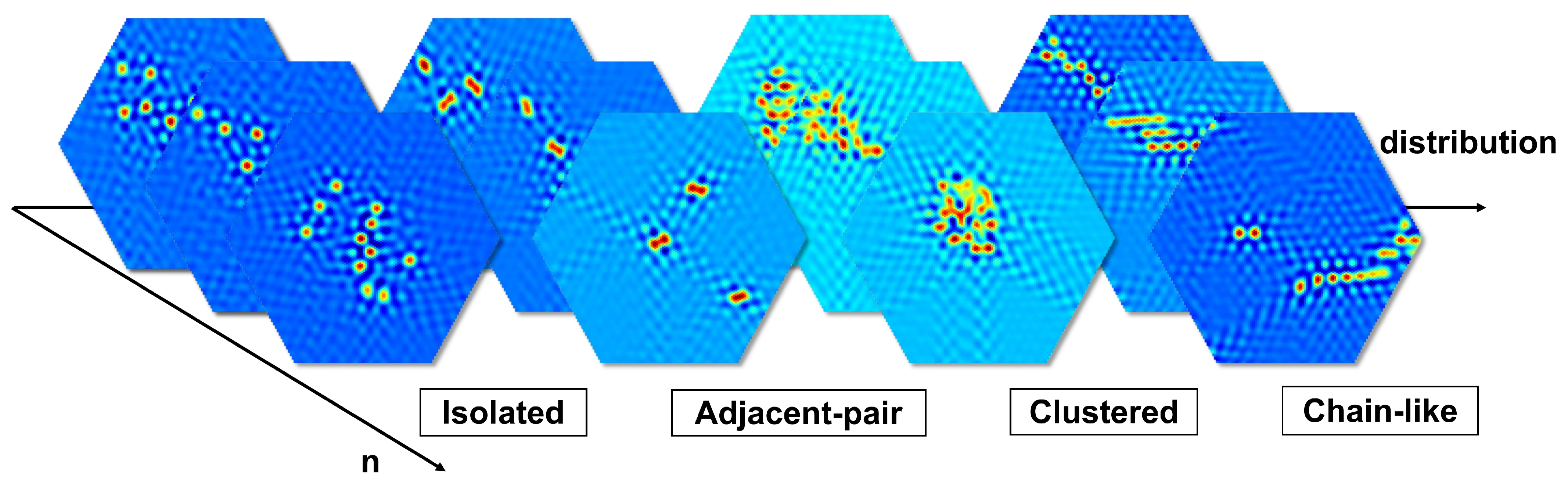
2.2. Emitter Distribution Patterns

To comprehensively evaluate the proposed detection method under different conditions, we design three emitter-distribution patterns, as illustrated in Figure 2. The isolated distribution pattern represents the most fundamental scenario where emitters are well separated from one another. The angular distance between any two emitters, measured in geographic longitude and latitude, satisfies $\left|p_i-p_j\right|⩾1°$. Under this condition, the intensity fields do not interfere, and the imaging result shows discrete high-intensity spots. This pattern is used to verify the basic detection capability of the algorithm for individual emitters. The adjacent-pair distribution pattern focuses on the core challenge of this work: separating conjoined emitters whose intensity fields overlap due to spatial proximity. For a pair of emitters with separation distance $\delta$ (again in geographic degrees), when $\delta$ falls below the imaging resolution, their brightness-temperature distributions merge into a single connected structure. To quantitatively assess the algorithm’s ability to resolve such conjoined emitters, three subsets are defined with progressively larger separations: $\delta \in [0.5,0.55]°$, $[0.55,0.6]°$, and $[0.6,0.7]°$, ranging from difficult to relatively easy. The complex distribution pattern simulates the irregular deployment of emitters in real-world electromagnetic environments. It is further divided into clustered and chain-like subtypes, but both are defined purely by geographic angular relations rather than by signal intensity. In the clustered subtype, emitters gather into one or several high-density regions, with intra-cluster angular distances between $0.5°$ and $1.0°$ and inter-cluster distances between $2°$ and $5°$. This mimics dense deployments such as urban communication hubs. In the chain-like subtype, emitters are arranged sequentially along a preferred direction with a step size also between $0.5°$ and $1.0°$, while the direction retains memory from one step to the next. This simulates the trajectory of a moving emitter or a linear array. Together, these two subtypes reflect the variety of spatial configurations that may occur in practice, and they are used to test the algorithm’s robustness under realistic complexity.

Overall, the three patterns are independent of each other. The isolated pattern validates basic single-emitter detection, the adjacent-pair pattern tests the ability to resolve overlapping emitters, which is the main contribution of this work, and the complex pattern evaluates performance under realistic electromagnetic scenarios.

3. Method

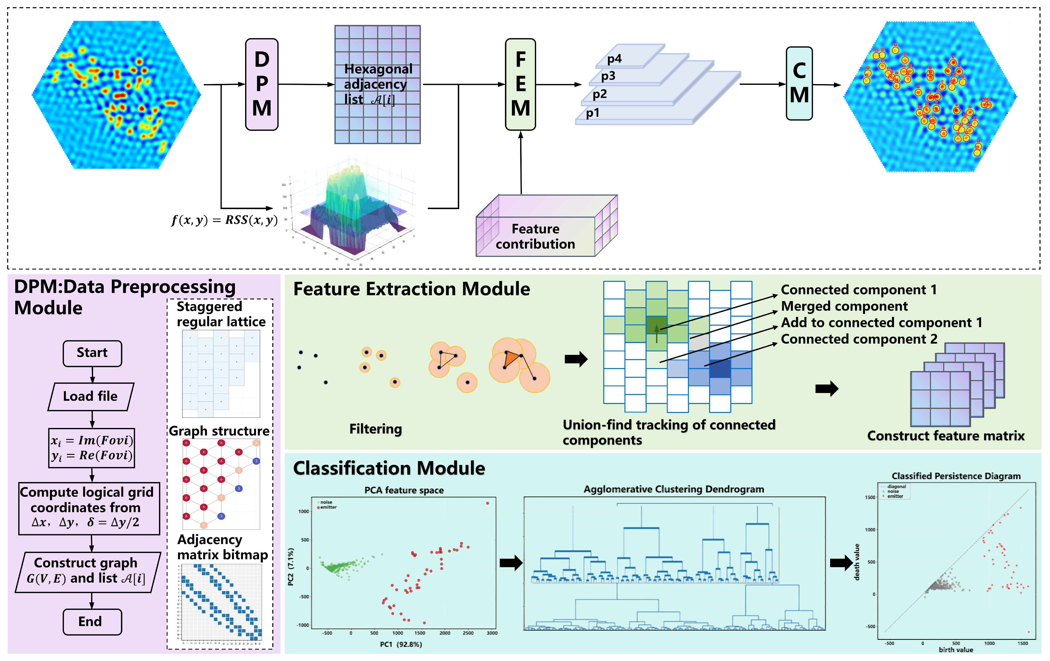
The overall workflow of the proposed emitter-detection method for REMs based on improved persistent homology is illustrated in Figure 3. It comprises three modules: data preprocessing, topological-feature extraction, and unsupervised classification. First, for the hexagonal-staggered-grid REM data generated by the spaceborne synthetic-aperture radiometer, the sampling points are mapped to a graph structure $G=(V,E)$ by utilizing the geometric prior of the grid. Each vertex carries a brightness-temperature attribute, and edges are defined by the six-neighborhood relationship, thereby establishing the foundation for subsequent topological analysis. On this basis, persistent-homology theory is introduced, with the brightness-temperature value serving as the filter function to construct a filtration sequence. The birth, death, and merging events of zero-dimensional connected components are tracked, and eight topological features—including persistence, birth value, neighborhood statistics, and merging proportion—are extracted for each component. To address the deficiency of conventional persistent homology, which relies solely on persistence and is consequently prone to missed detections of adjacent emitters, we design multidimensional features to characterize the distinctions among emitters and noise in terms of stability, intensity, and local patterns. Finally, agglomerative clustering with Ward linkage is employed to perform unsupervised binary classification on components with high birth values. Based on physical interpretation, the high-persistence cluster is automatically mapped to emitters, while the low-persistence cluster is mapped to noise. This method requires no annotated data, achieving adaptive detection solely by exploiting the topological structure of the radio-environment map, and attains a favorable balance between computational efficiency and detection accuracy.

3.1. Data Preprocessing

Persistent-homology computation is conventionally performed on point-cloud data through the construction of Rips complexes, wherein a distance threshold $ϵ$ is set, and point pairs with distances less than $ϵ$ are connected to form edges, thereby generating simplicial complexes of various dimensions [54,55,56]. The radio-environment-map data acquired by the spaceborne synthetic-aperture radiometer possess an explicitly defined hexagonal-staggered-grid structure, with the spatial positions of sampling points uniquely determined by the grid parameters $\mathrm{\Delta }x$, $\mathrm{\Delta }y$, and $\delta$. This paper fully exploits this structural prior by mapping the point cloud to a graph structure during the preprocessing stage.

The radio-environment-map data are stored in complex form, with each sampling point corresponding to a spatial position and its brightness-temperature value. Let the total number of sampling points be N, the complex coordinate of the i-th point be ${\mathrm{Fov}}_i=y_i+\mathrm{j}{x}_i$, and its brightness-temperature value be $T_i$. These sampling points are arranged on a hexagonal staggered grid: the horizontal column spacing is $\mathrm{\Delta }x$, the vertical row spacing is $\mathrm{\Delta }y$, and odd-indexed columns exhibit a vertical offset of $\delta =\mathrm{\Delta }y/2$ relative to even-indexed columns. The physical coordinates are extracted from the complex numbers as $x_i=Im\left({\mathrm{Fov}}_i\right)$, $y_i=Re\left({\mathrm{Fov}}_i\right)$, yielding the set of sampling points $(x_i,y_i,T_i)$, $i=1,\dots ,N$. Each point is mapped to a logical grid column index $c_i$ and row index $r_i$ based on the grid geometric parameters. The column index is

$$c_i=⌊{\displaystyle \frac{x_i}{\mathrm{\Delta }x}}+0.5⌋$$

(6)

The row index is

$$r_i=\left\{\begin{array}{cc}⌊{\displaystyle \frac{y_i}{\mathrm{\Delta }y}}+0.5⌋,\hfill & \mathrm{even}\mathrm{columns}\hfill \\ ⌊{\displaystyle \frac{y_i-\delta }{\mathrm{\Delta }y}}+0.5⌋,\hfill & \mathrm{odd}\mathrm{columns}\hfill \end{array}\right.$$

(7)

The reconstruction error of this mapping is controlled at the order of ${10}^{-6}$. For invalid points where coordinates or brightness-temperature values are NaN or Inf, a validity mask $\mathcal{V}=\{i\mid x_i,y_i,T_i\mathrm{are}\mathrm{all}\mathrm{finite}\}$ is constructed, and $N_{\mathrm{valid}}=\left|\mathcal{V}\right|$ is recorded. In the hexagonal grid, each point has at most six neighbors, and the neighborhood offsets depend on the column parity. Let the logical coordinates of point i be $(c_i,r_i)$. If $c_i$ is even, the neighbor offsets are

$$(0,1),(0,-1),(-1,0),(1,0),(-1,-1),(1,-1)$$

(8)

If $c_i$ is odd, the offsets are

$$(0,1),(0,-1),(-1,1),(1,1),(-1,0),(1,0)$$

(9)

For each valid point, the theoretical coordinates of each neighbor are computed. If a corresponding valid point j exists, an edge $(i,j)$ is added to the adjacency list, ultimately yielding the adjacency list $\mathcal{A}\left[i\right]$.

Through the aforementioned preprocessing, the raw radio-environment-map data are transformed into a graph structure $G=(V,E)$, where the vertex set V corresponds to the valid sampling points, each vertex i carries the brightness-temperature attribute $T_i$, and the edge set E is defined by the hexagonal-adjacency relationships. The emitter-detection problem is, thus, converted into a topological analysis problem on the graph structure, providing a unified mathematical foundation for the subsequent persistent-homology analysis.

3.2. Feature-Extraction Module

The feature-extraction module, based on persistent-homology theory, extracts multidimensional features reflecting the topological stability of emitters from the hexagonal adjacency list obtained during preprocessing. Persistent homology is employed to investigate the evolution of topological features as a parameter varies. Its core involves defining a filter function $f:V\to \mathbb{R}$; in this paper, $f\left(i\right)=T_i$ is adopted, and the vertices are sorted. Let a threshold be denoted by $\alpha$, and define the sublevel set $L_{\alpha }=\{v\in V\mid f\left(v\right)\ge \alpha \}$. As $\alpha$ decreases from $T_{max}$ to $T_{min}$, $L_{\alpha }$ expands from the empty set to the entire vertex set, forming a filtration sequence as follows:

$$\varnothing =L_{T_{\max }}\subseteq L_{T_2}\subseteq \cdots \subseteq L_{T_{\min }}=V.$$

(10)

The homology groups of each $L_{T_i}$ are computed, and their dimensions correspond to the k-dimensional Betti numbers ${\beta }_k$: ${\beta }_0$ denotes the number of connected components, ${\beta }_1$ denotes the number of loops, and ${\beta }_2$ denotes the number of voids. As this paper focuses on emitter detection, only the zero-dimensional topological structure—namely, the variation in ${\beta }_0$ with the threshold—requires analysis. During this process, new connected components continuously emerge, and existing components merge with one another, leading to the disappearance of some components. The method is detailed in Algorithm 1.

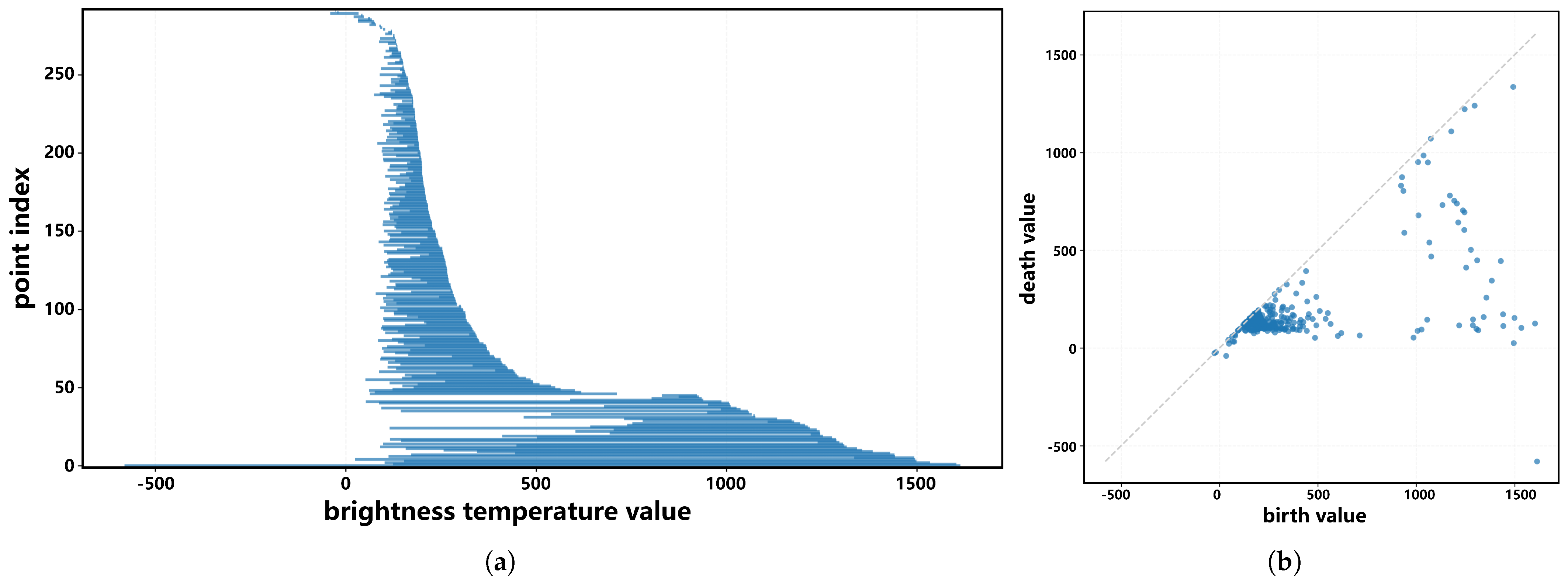
Upon execution of Algorithm 1, a set of birth–death pairs $P=(b_i,d_i)$ is obtained. Each pair $(b_i,d_i)$ corresponds to a connected component that once existed independently, and its persistence $\mathrm{pers}=b_i-d_i$ reflects the range of stable existence of that component within the intensity domain. Visualizations of persistent homology commonly include Persistence Barcodes (PB) and Persistence Diagrams (PD), as illustrated in Figure 4. The set P can be visualized as a PB, wherein each component is represented as a horizontal segment with the left endpoint at the birth value b and the right endpoint at the death value d; the segment length corresponds to the persistence. Alternatively, it can be visualized as a PD, where points $(b,d)$ are plotted on a two-dimensional plane; the vertical distance of a point from the diagonal line $b=d$ is precisely its persistence. In a PD, when emitters are distributed in isolation, points situated farther from the diagonal—corresponding to components with higher persistence—represent emitters, whereas points near the diagonal correspond to noise.

However, when two emitters with comparable intensities are spatially proximate, their connected components merge early during the construction of the union-find structure. The merged components exhibit short persistence and are prone to being misclassified as noise, thereby leading to missed detections. Consequently, distinguishing emitters from noise cannot rely solely on persistence; other features must also be considered. We construct an eight-dimensional feature vector for each birth–death pair based on an analysis of feature contributions, and the specific features are enumerated in

Table 1. Features for emitter-noise classification.

Category	Feature	Physical Interpretation
Stability	Persistence $p=b-d$	Lifespan of the component
	Birth value b	Intensity of the component
	Normalized persistence $p/b$	Relative stability
Neighborhood Statistics	Mean birth value of neighbors ${\mu }_{\mathrm{nbr}}$	Local background intensity
	Maximum birth value among neighbors ${max}_{\mathrm{nbr}}$	Neighborhood peak value
	Standard deviation of neighbors ${\sigma }_{\mathrm{nbr}}$	Degree of local fluctuation
Merging Feature	Merging proportion $\rho$	Intensity ratio relative to the surviving component
Global Statistic	Normalized birth value $z=(b-{\mu }_b)/{\sigma }_b$	Relative global intensity

.

Algorithm 1 Topological-Feature Extraction Based on Persistent Homology

Require:  Graph $G=(V,E)$, vertex brightness-temperature values $T:V\to \mathbb{R}$ Ensure:  Set of birth–death pairs $P=(b_i,d_i)$, set of merging events $\mathcal{M}=({\rho }_j,b_j)$   1: Sort V in descending order of $T\left(v\right)$ to obtain the sequence $v_1,v_2,\dots ,v_N$    ▹ Construct the filtration sequence   2: Initialize Union-Find $UF$, vertex state array $\mathrm{active}\left[v\right]\leftarrow \mathrm{False}$   3: Initialize $P\leftarrow \varnothing$, $\mathcal{M}\leftarrow \varnothing$   4: for $i=1$ to N do   5:     $v\leftarrow v_i$, $\mathrm{active}\left[v\right]\leftarrow \mathrm{True}$          ▹ Activate the current vertex   6:     Collect all already activated neighbors of v: $\mathcal{N}=\{u\in \mathrm{adj}(v)\mid \mathrm{active}[u\left]\right\}$   7:     if $\mathcal{N}=\varnothing$ then   8:         $UF.\mathrm{create}\left(v\right)$, create a new component C, $\mathrm{birth}\left(C\right)\leftarrow T\left(v\right)$      ▹ Birth event   9:     else 10:         Obtain the representatives of each component in $\mathcal{N}$, deduplicate to obtain the set $\{r_1,\dots ,r_m\}$ 11:         Sort $r_{\left(1\right)},\dots ,r_{\left(m\right)}$ in descending order of $\mathrm{birth}\left(r_k\right)$▹ Component with the largest birth value takes precedence 12:         $UF.\mathrm{union}(v,r_{\left(1\right)})$, merge v into the component of $r_{\left(1\right)}$ 13:         for $k=2$ to m do    ▹ Process the remaining components, record death events 14:              $b_m\leftarrow \mathrm{birth}\left(r_{\left(k\right)}\right)$, $b_a\leftarrow \mathrm{birth}\left(r_{\left(1\right)}\right)$ 15:              $\rho \leftarrow b_m/b_a$, $\mathcal{M}\leftarrow \mathcal{M}\cup \left\{(\rho ,b_m)\right\}$        ▹ Record the merging proportion 16:              $P\leftarrow P\cup \left\{(b_m,T\left(v\right))\right\}$, mark $r_{\left(k\right)}$ as dead               ▹ Death event 17:              $UF.\mathrm{union}(r_{\left(1\right)},r_{\left(k\right)})$                      ▹ Merge the components 18:         end for 19:     end if 20: end for 21: Mark the final surviving components with a death value of $T_{min}$ and add them to P 22: return P, $\mathcal{M}$

3.3. Classification Module

Given that emitters typically exhibit higher persistence, larger birth values, and stable merging patterns, whereas noise points perform weakly across these indicators, the two classes of features should manifest separability within the feature space. We employ agglomerative clustering (AC) to achieve unsupervised classification [57,58]. This algorithm merges similar samples iteratively in a bottom-up manner, generating a hierarchical tree, and yields the final partition by specifying the number of clusters as $k=2$.

To eliminate dimensional discrepancies, each feature dimension is standardized using RobustScaler:

$${\tilde{x}}_{ij}={\displaystyle \frac{x_{ij}-median\left(x_j\right)}{IQR\left(x_j\right)}}$$

(11)

where $IQR\left(X_j\right)$ denotes the interquartile range of the j-th dimension. The distance between samples adopts the Euclidean distance:

$$d({\mathbf{x}}_i,{\mathbf{x}}_j)={\parallel {\mathbf{x}}_i-{\mathbf{x}}_j\parallel }_2$$

(12)

The inter-cluster distance employs Ward linkage, the objective of which is to minimize the increment in within-cluster variance following each merger. Let clusters A and B have sample sizes $n_A$ and $n_B$, centroids ${\overline{\mathbf{x}}}_A$ and ${\overline{\mathbf{x}}}_B$, respectively, and let the centroid of the merged cluster be ${\overline{\mathbf{x}}}_{AB}$. The incremental sum of squares error upon merging is

$$\mathrm{\Delta }E={\displaystyle \frac{n_A{n}_B}{n_A+n_B}}{∥{\overline{\mathbf{x}}}_A-{\overline{\mathbf{x}}}_B∥}^2$$

(13)

Ward linkage selects the pair of clusters that minimizes $\mathrm{\Delta }E$ for merging, thereby ensuring the compactness of the hierarchical clustering [59]. Based on physical interpretation, the number of clusters is fixed as $k=2$. After obtaining the initial cluster labels ${\ell }_i\in \{0,1\}$, it is necessary to align the clusters with their physical meaning. We utilize the prior knowledge that emitters possess high persistence by computing the mean persistence of each cluster:

$${\overline{p}}_c={\displaystyle \frac{1}{|C_c|}}\sum _{i\in C_c}(b_i-d_i)$$

(14)

The cluster with the larger $\overline{p}$ is designated as an emitter (label 0), while the cluster with the smaller $\overline{p}$ is designated as noise (label 1).

4. Experiments

4.1. Experimental Setup

Dataset: A self-constructed simulated dataset of spaceborne REMs is utilized, comprising two formats. Dataset 1 contains five test sets: test1 (isolated distribution), test2 (adjacent-pair with $\delta \in [0.6,0.7]°$), test3 (adjacent-pair with $\delta \in [0.55,0.6]°$), test4 (adjacent-pair with $\delta \in [0.5,0.55]°$), and test5 (complex distribution), each comprising 500 samples. Dataset 2 comprises a training set of 1000 samples and the same five test sets as in Dataset 1, annotated with bounding box labels in the YOLO format.

Evaluation Metrics: Precision measures the fraction of correctly detected emitters among all detections:

$$\mathrm{Precision}={\displaystyle \frac{\mathrm{TP}}{\mathrm{TP}+\mathrm{FP}}}$$

(15)

Recall measures the fraction of correctly detected emitters among all ground-truth emitters:

$$\mathrm{Recall}={\displaystyle \frac{\mathrm{TP}}{\mathrm{TP}+\mathrm{FN}}}$$

(16)

F1 Score is the harmonic mean of precision and recall:

$$F1=2·{\displaystyle \frac{\mathrm{Precision}·\mathrm{Recall}}{\mathrm{Precision}+\mathrm{Recall}}}$$

(17)

A greedy matching strategy is adopted with a distance threshold of $0.03$ rad. A detected emitter is considered correct only if its Euclidean distance to a ground-truth emitter is below this threshold.

Experimental Environment and Parameter Settings: All experiments were performed on a server equipped with an Intel Core i9-14900HX (Intel Corporation, Santa Clara, CA, USA) processor and an NVIDIA GeForce RTX 4070 (NVIDIA Corporation, Santa Clara, CA, USA) graphics card. Data simulation was carried out in MATLAB R2024b (The MathWorks, Inc., Natick, MA, USA). The compared methods were implemented in PyCharm Community Edition 2024.3 using Python 3.8, PyTorch 1.10, scikit-learn 1.1.0, and other standard libraries.

4.2. Comparison with Existing Methods

For image-processing techniques, Wavelet [20], Morphology [21], Statistical [31], and Threshold [25] were selected. For object-detection techniques, YOLOv13 [36] and its improved variant YOLOv13_FreqFusion [45], both in their nano versions, were selected. To ensure fair comparison, all compared methods are reproduced according to the original literature or obtained from publicly available repositories (e.g., the Ultralytics YOLO implementation at https://github.com/iMoonLab/yolov13 (accessed on 28 April 2026), and the FreqFusion module at https://github.com/ying-fu/FreqFusion (accessed on 28 April 2026)), and optimal parameter configurations are adopted for all. The Precision, Recall, and F1 Score metrics obtained by testing the existing methods on the constructed dataset are presented in

Table 2. Comparison of Precision.

Algorithm	Test1	Test2	Test3	Test4	Test5	Average
PH-AC (proposed)	1.0000	0.9981	0.9929	0.9983	0.9833	0.9945
Wavelet	0.9990	0.9711	0.9784	0.9889	0.9835	0.9842
Morphology	0.9948	0.9307	0.9408	0.9539	0.8758	0.9392
Statistical	0.9976	0.9414	0.9193	0.8988	0.9256	0.9365
Threshold	1.0000	1.0000	1.0000	1.0000	0.9961	0.9992
YOLOv13	0.9958	0.9787	0.9881	0.9877	0.9147	0.9730
YOLOv13_FreqFusion	0.9968	0.9796	0.9896	0.9899	0.9229	0.9758

Note: For each test set, metrics marked in red indicate first place, blue indicate second place, and green indicate third place. The average column also highlights the top three overall averages in red (1st), blue (2nd), and green (3rd).

,

Table 3. Comparison of Recall.

Algorithm	Test1	Test2	Test3	Test4	Test5	Average
PH-AC (proposed)	1.0000	0.8717	0.9350	0.9633	0.8948	0.9330
Wavelet	0.9982	0.6167	0.7183	0.8158	0.6741	0.7646
Morphology	0.9958	0.7833	0.8742	0.9308	0.8137	0.8796
Statistical	0.9992	0.7233	0.8067	0.8883	0.6759	0.8187
Threshold	0.9904	0.5467	0.6425	0.7767	0.6684	0.7249
YOLOv13	0.9970	0.9633	0.9800	0.9867	0.8891	0.9632
YOLOv13_FreqFusion	0.9980	0.9733	0.9783	0.9867	0.8980	0.9669

Note: For each test set, metrics marked in red indicate first place, blue indicate second place, and green indicate third place. The average column also highlights the top three overall averages in red (1st), blue (2nd), and green (3rd).

and

Table 4. Comparison of F1 Score.

Algorithm	Test1	Test2	Test3	Test4	Test5	Average
PH-AC (proposed)	1.0000	0.9306	0.9631	0.9805	0.9370	0.9622
Wavelet	0.9986	0.7543	0.8284	0.8941	0.7999	0.8551
Morphology	0.9953	0.8507	0.9063	0.9422	0.8436	0.9076
Statistical	0.9984	0.8181	0.8593	0.8935	0.7813	0.8701
Threshold	0.9952	0.7069	0.7823	0.8743	0.8000	0.8317
YOLOv13	0.9964	0.9709	0.9840	0.9872	0.9017	0.9680
YOLOv13_FreqFusion	0.9974	0.9764	0.9840	0.9883	0.9103	0.9713

Note: For each test set, metrics marked in red indicate first place, blue indicate second place, and green indicate third place. The average column also highlights the top three overall averages in red (1st), blue (2nd), and green (3rd).

.

As the harmonic mean of Precision and Recall, the F1 score provides a comprehensive measure of emitter-detection performance. According to the average F1 values computed from the five test sets in Table 4, the proposed PH-AC method achieves an average F1 of 0.9622, which is 5.46% higher than that of the best traditional image-processing method. In comparison with the supervised YOLO-based detectors, PH-AC lags by only 0.58% behind YOLOv13 and 0.91% behind YOLOv13_FreqFusion, despite requiring no annotated data. These results demonstrate that the proposed unsupervised topological approach attains competitive detection efficacy against state-of-the-art supervised methods while maintaining a clear advantage over all traditional image-processing techniques.

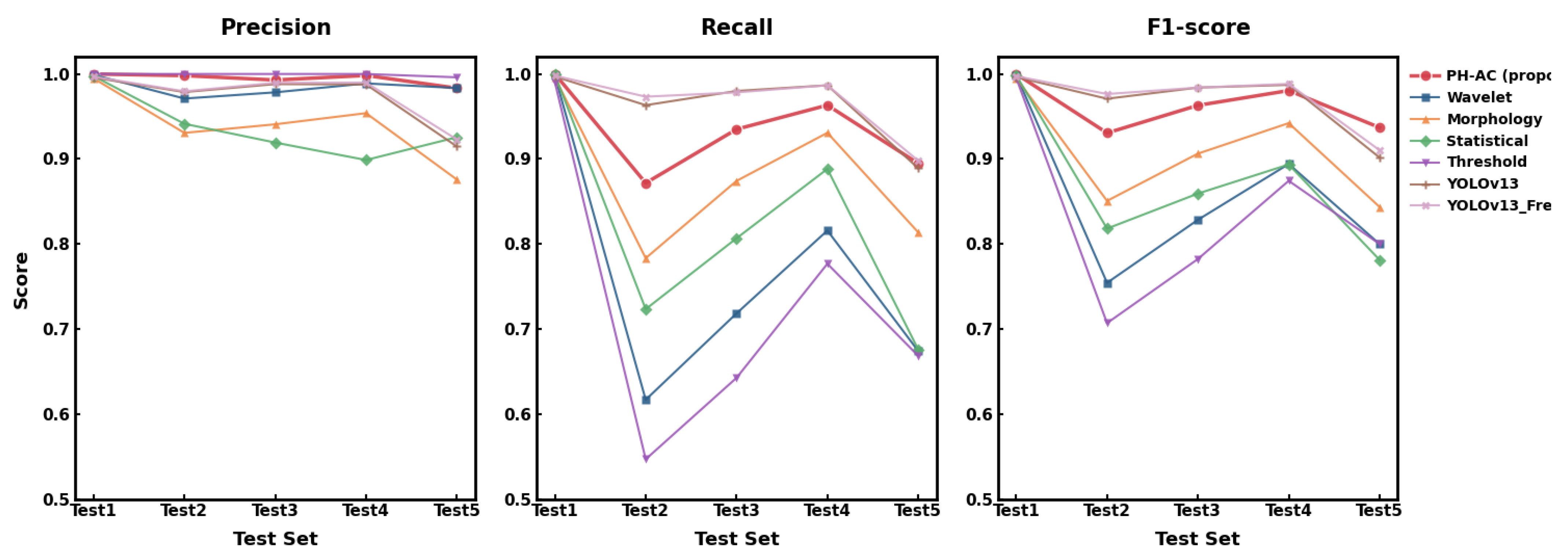
Figure 5 provides a more intuitive comparison of the test results. The proposed PH-AC method extracts zero-dimensional topological features via persistent homology, constructs multidimensional features, and achieves unsupervised classification through agglomerative clustering. In the isolated distribution scenario, the PH-AC method attains a perfect score of 1.0000 for Precision, Recall, and F1 Score, making it the sole algorithm to achieve flawless performance. In adjacent-pair scenarios, by tracking the merging events and merging proportions of connected components, the PH-AC method effectively resolves the challenge of separating “conjoined” structures arising from the superposition of intensity fields of adjacent emitters, surpassing all traditional image-processing methods. In the adjacent-pair scenarios, the F1 score of PH-AC is approximately 2–3% lower on average than that of the supervised YOLO series; however, in test4, with larger spacing, the gap narrows to within 0.7%. More importantly, PH-AC requires no annotated data, whereas YOLO depends on a large corpus of precisely labeled radio-environment-map samples. In the complex electromagnetic environment, PH-AC achieves an F1 score as high as 0.9370, which not only significantly outperforms all traditional image-processing methods but also exceeds supervised YOLOv13 by 3.91% and YOLOv13_FreqFusion by 2.93%. Simultaneously, its Precision of 0.9833 and Recall of 0.8948 exhibit the most favorable balance, while the YOLO series yields more false positives in complex environments. It is worth noting that while the Threshold method achieves perfect or near-perfect Precision, its Recall is extremely low. This indicates that the Threshold method tends to detect only the most prominent emitters while missing a large number of valid emitters, resulting in a severe precision–recall trade-off. Consequently, despite its high Precision, the low Recall renders it unsuitable for reliable emitter detection in complex electromagnetic environments. In contrast, the proposed PH-AC method achieves a substantially higher Recall and maintains a well-balanced precision–recall trade-off, effectively overcoming the limitation of threshold-based approaches.Furthermore, the PH-AC method demonstrates exceptional robustness: from isolated distribution to complex electromagnetic environments, its F1 Score remains consistently above 0.93, exhibiting the smallest performance degradation. In contrast, the F1 Score of the compared Wavelet method plummets from 0.9986 to 0.7999, further corroborating the stability and superiority of the proposed method.

4.3. Computational-Complexity Comparison and Analysis

To objectively evaluate the computational efficiency of the proposed PH-AC method, we counted the number of floating-point operations (FLOPs) and the number of comparisons (COMP). FLOPs reflect the dependence of an algorithm on floating-point units, while the COMP indicates the pressure on branch prediction and data comparison. Both metrics are independent of hardware platforms and can fairly compare the theoretical computational load of different algorithms. The time and space complexities are expressed in Big-O notation to qualitatively describe how the algorithm scales with input size. Based on the real data scales, where the number of valid sampling points is 11,773, the gridded size is 12,000 pixels, and the number of connected components for PH-AC is 300, we evaluated five traditional emitter-detection algorithms. The YOLO-based object detectors were profiled using the PyTorch library thop. The results are presented in

Table 5. Computational-complexity comparison of different algorithms.

Algorithm	FLOPs	COMP	Parameters	Time Complexity	Space Complexity
PH-AC (proposed)	2.25 M	182.24 K	0	$O(NlogN+M^{2}logM)$	$O(N+M·d)$
Wavelet	4.73 M	29.71 M	0	$O(N_{\mathrm{grid}}·L·F)$	$O(N_{\mathrm{grid}}·L)$
Morphology	74.40 K	29.16 M	0	$O(N_{\mathrm{grid}}·K^2)$	$O\left(N_{\mathrm{grid}}\right)$
Statistical	2.25 M	28.45 M	0	$O\left(N_{\mathrm{grid}}\right)$	$O\left(N_{\mathrm{grid}}\right)$
Threshold	538.69 K	28.75 M	0	$O(L^2·K+N_{\mathrm{grid}})$	$O\left(N_{\mathrm{grid}}\right)$
YOLOv13	6.4 G	—	2.36 M	$O\left(HWC\right)$	$O\left(\mathrm{parameters}\right)$
YOLOv13_FreqFusion	5.9 G	—	2.38 M	$O\left(HWC\right)$	$O\left(\mathrm{parameters}\right)$

Note: “—” indicates that the metric is not applicable for deep learning models due to their different computational paradigms. N denotes the number of sampling points, M the number of connected components in PH-AC, L the number of decomposition levels in wavelet transform, F the filter length, K the structuring element size in morphology, $N_{\mathrm{grid}}$ the number of grid pixels, H, W, C the height, width, and channels of the input to YOLO models, and d the feature dimension.

.

The advantages of the proposed method are clearly shown in Table 5. Among traditional image-processing algorithms, PH-AC has a floating-point operation count comparable to that of the Statistical method, lower than that of Wavelet, and slightly higher than that of Morphology. More importantly, its comparison count is two orders of magnitude lower than that of all grid-based conventional methods. This is because PH-AC directly operates on the original scatter points and completely avoids the massive comparisons caused by gridding and hole filling. Consequently, PH-AC exerts minimal branch-prediction pressure and is more suitable for efficient execution on general-purpose CPUs. In terms of time complexity, PH-AC achieves $O(NlogN+M^{2}logM)$, which is more favorable than Wavelet’s $O(N_{\mathrm{grid}}·L·F)$ and Morphology’s $O(N_{\mathrm{grid}}·K^2)$, when the number of components M is much smaller than the number of points N. Its space complexity $O(N+M·d)$ is also linear in the input size, avoiding the quadratic overhead of grid-based methods. Compared to YOLOv13-type algorithms, the FLOPs of PH-AC is approximately three orders of magnitude lower. Moreover, both YOLO models have over 2.36 million parameters, whereas PH-AC has no trainable parameters. Despite the three-order-of-magnitude difference in computational cost, experiments demonstrate that PH-AC achieves accuracy and recall comparable to those of YOLO in the emitter-detection task.

In summary, the proposed PH-AC method strikes a balanced optimization between floating-point operations and comparisons among conventional techniques, and notably reduces the number of comparisons. At the same time, it attains detection performance similar to that of deep learning models while requiring less than one three-thousandth of their floating-point operations. These characteristics make PH-AC highly suitable for real-time emitter detection on computationally constrained platforms such as spaceborne, airborne, or handheld devices.

4.4. Method Testing on Complex Electromagnetic-Environment Samples

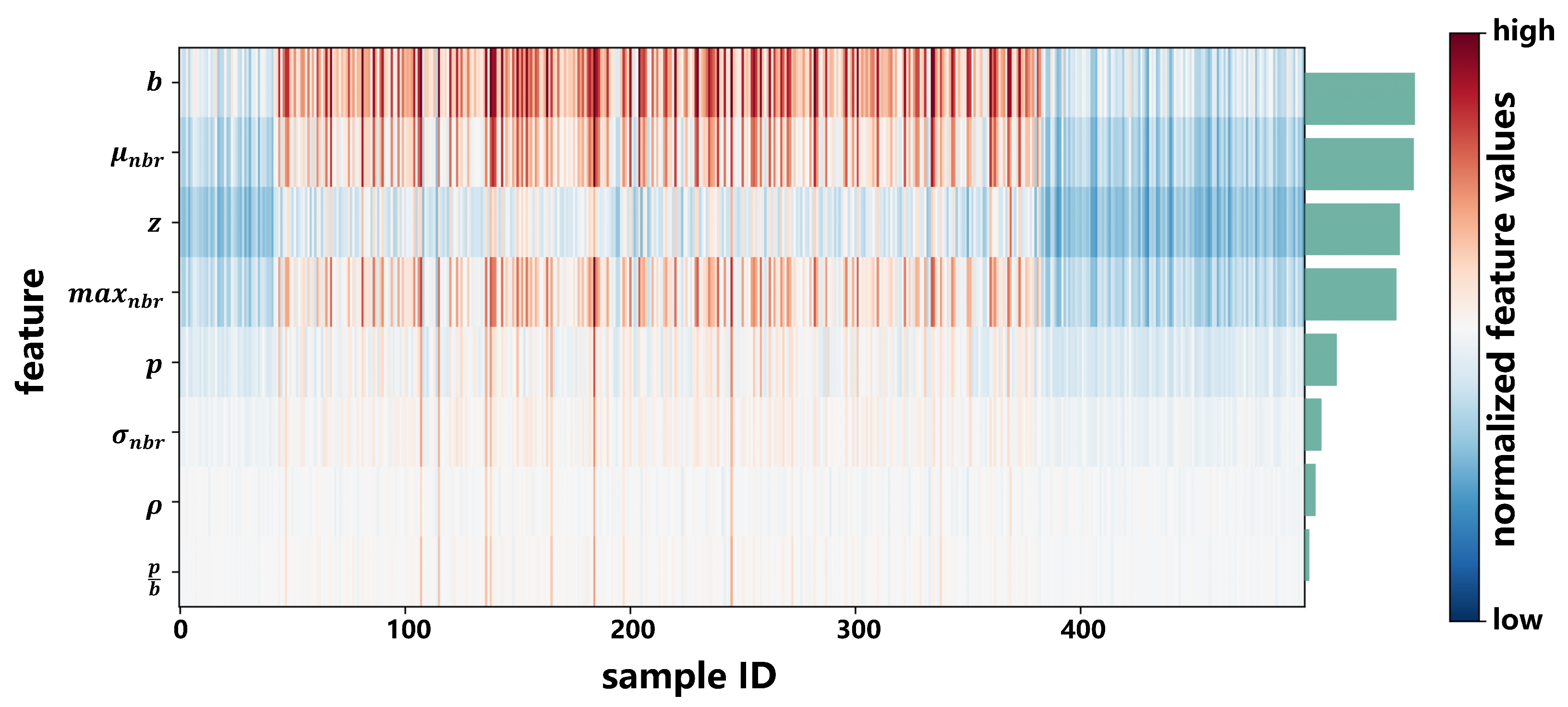
Since conventional persistent-homology algorithms rely solely on persistence to distinguish significant features from noise, they are prone to missed detections of merged adjacent emitters or weak emitters. Consequently, we analyze the eight-dimensional features mentioned previously by performing feature-contribution analysis on 500 samples from test5 in Dataset 1, generating a SHAP heatmap as illustrated in Figure 6, where red indicates promotion of emitter classification and blue indicates promotion of noise classification. Stronger color intensity signifies greater importance of the feature for classification within these samples.

To evaluate the detection capability of the proposed method in complex electromagnetic environments, we designed a simulation scenario, as illustrated in Figure 7: 46 L-band fixed-communication base-station ground emitters with a center frequency of 1.5 GHz are non-uniformly distributed across Uzbekistan and the surrounding Aral Sea region. In the resulting spaceborne-radio-environment map, active emitters appear as yellow–orange–red hotspots, while low-activity background is rendered in blue. This color mapping provides an intuitive visual indication of emitter locations. Among the 46 emitters, isolated emitters—such as the station located at $57.8°$E, $44.25°$N northwest of the Aral Sea—are separated from their nearest neighbors by distances exceeding 167 km. Adjacent pairs exhibit separations ranging from 40 to 70 km, wherein intensity fields severely overlap, forming a “conjoined” structure. In clustered regions, eight emitters are concentrated within the area spanning $63.2°$E to $63.8°$E and $41.4°$N to $43.0°$N, with a minimum intra-cluster separation of approximately 33 km, thereby simulating dense deployment scenarios in urban areas or military bases. A chain-like distribution extends meridionally along $65°$E to $66.5°$E, comprising 12 emitters arranged at approximately equal intervals of about 55 to 78 km, simulating the trajectory of a moving emitter or a linear array.

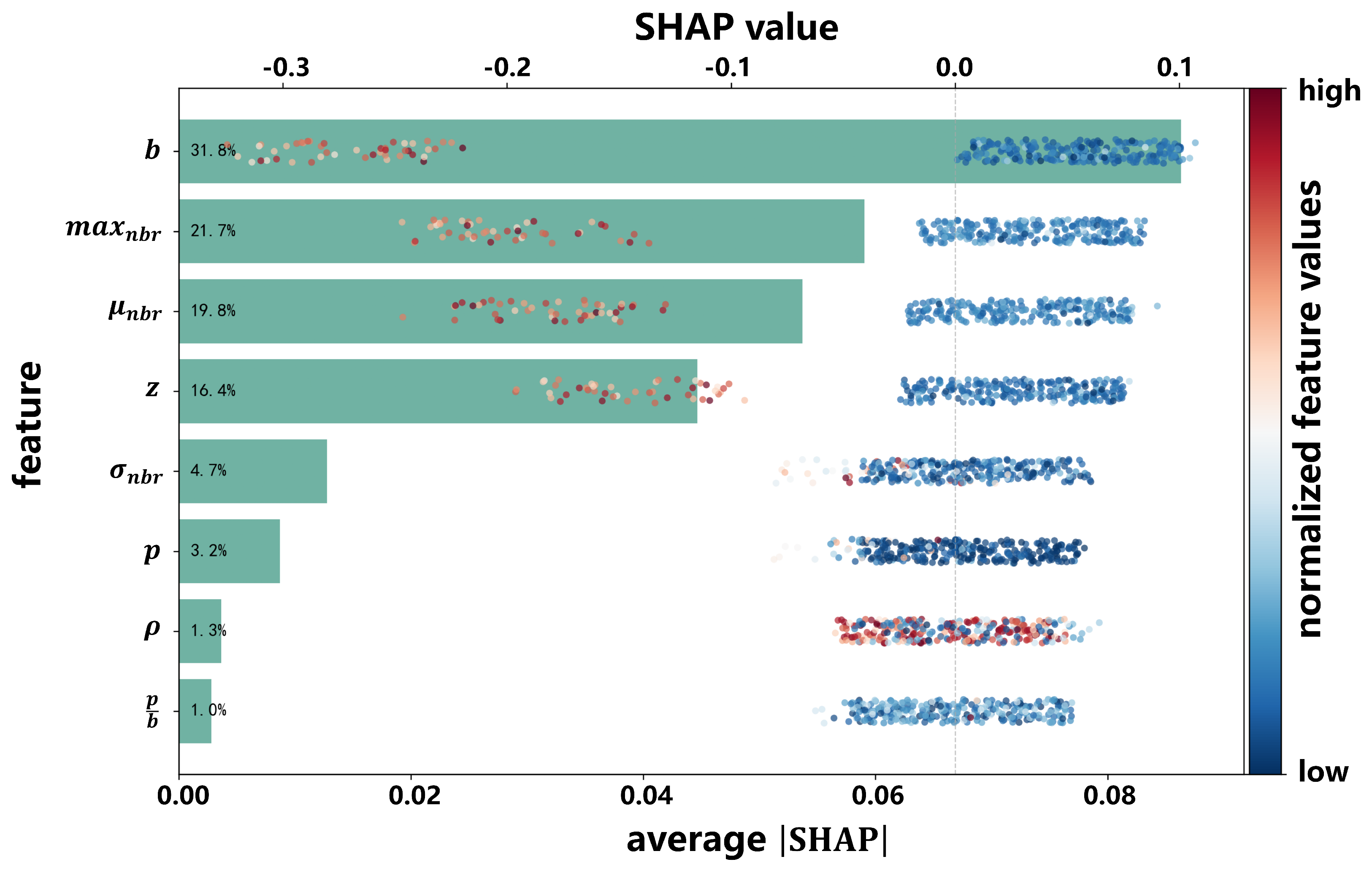
Subsequently, preprocessing and feature extraction were performed on the radio-environment map of this scenario, and SHAP analysis was employed to assess the classification contribution of each feature. Figure 8 presents a global explanation plot combining a bar chart and a beeswarm plot: the bar length denotes the ranking of feature importance; the horizontal position of the beeswarm points reflects the positive or negative contribution of the feature toward classifying an emitter or noise; and the color represents the magnitude of the feature value. It is evident that the birth value and neighborhood features play dominant roles in the classification of this sample.

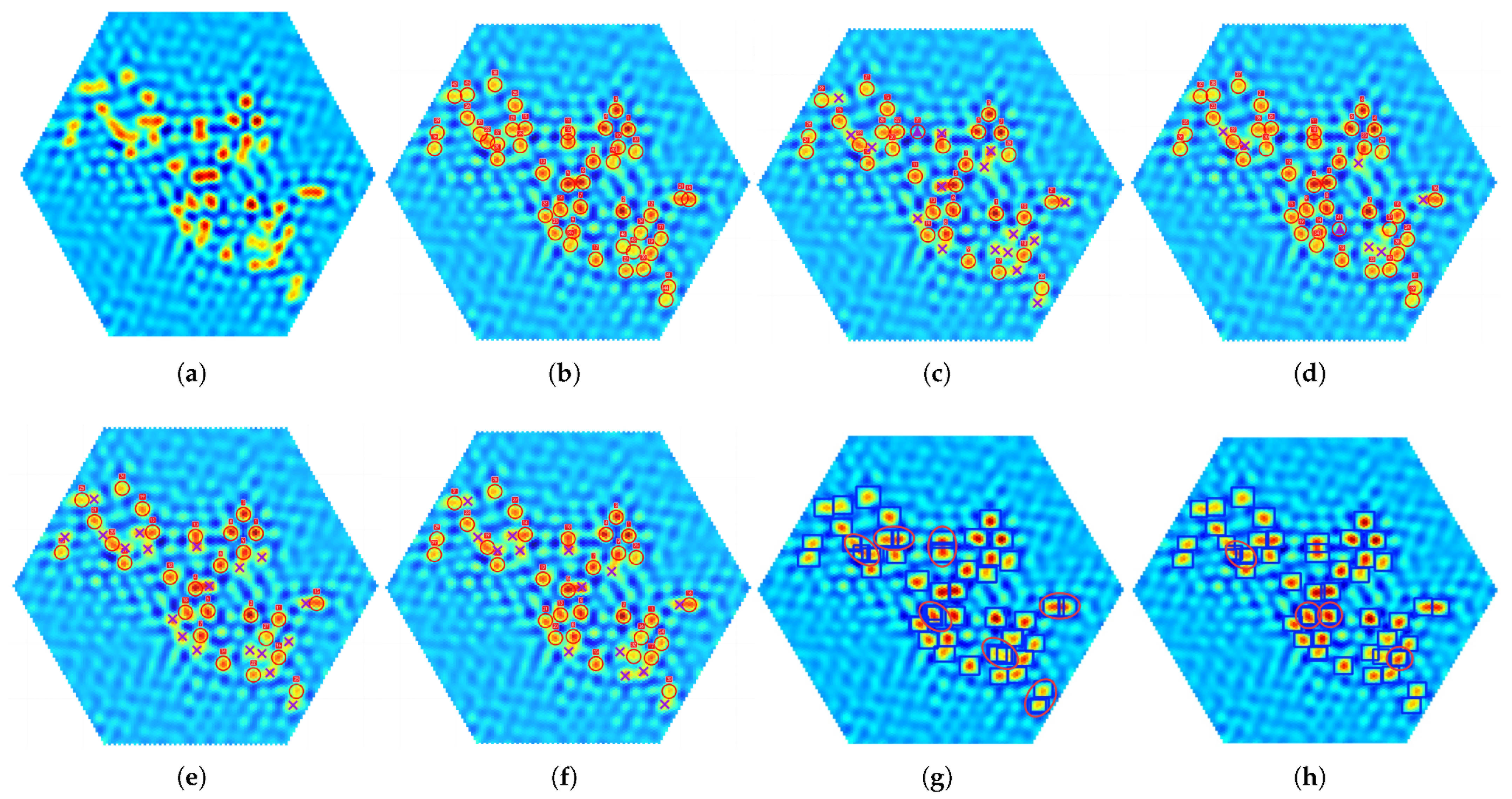
We subsequently tested the proposed method and existing state-of-the-art methods on this scenario sample, and the emitter-detection results are presented in

Table 6. Detection-performance comparison of the complex-electromagnetic-environment scenario with 46 emitters.

Method	FN	FP	TP	Precision	Recall	F1
PH-AC (Proposed)	0	0	46	1.0000	1.0000	1.0000
Wavelet	16	1	30	0.9677	0.6522	0.7794
Morphology	6	1	40	0.9756	0.8696	0.9194
Statistical	19	0	27	1.0000	0.5870	0.7398
Threshold	14	0	32	1.0000	0.6957	0.8205
YOLOv13	0	7	46	0.8679	1.0000	0.9293
YOLOv13_FreqFusion	0	4	46	0.9200	1.0000	0.9583

and Figure 9.

The quantitative results in Table 6 summarize the detection performance of all methods. The proposed PH-AC achieves perfect scores across all metrics, with zero missed emitters and zero false alarms, leading to an F1 score of 1.000. Traditional image-processing methods suffer from severe trade-offs: Wavelet misses 16 emitters and produces one false alarm; Morphology performs better with six misses and one false alarm; Statistical and Threshold methods avoid false alarms but miss 19 and 14 emitters, respectively, yielding low recall and F1 scores of around 0.74–0.82. Supervised deep learning detectors, YOLOv13 and its FreqFusion variant, achieve no misses but generate 7 and 4 false alarms, respectively, primarily in regions with adjacent emitters. Their F1 scores are 0.9293 and 0.9583, both lower than that of the proposed PH-AC. Notably, PH-AC attains this superior performance without requiring any annotated training data, a clear advantage over the YOLO series. Figure 9 visualizes the detection results, where the proposed method correctly identifies all 46 emitter locations without any false positives, while other methods exhibit missed detections or false alarms. The visualization corroborates the quantitative findings, confirming that PH-AC effectively balances missing and false alarms, achieving the highest F1 score through an unsupervised topological approach.

4.5. Ablation Study

To further validate the effectiveness of each core component within the proposed method, an ablation study was conducted on the complex electromagnetic environment test set, test5. Three variants were established for the experiments: PH: employing only the conventional persistent-homology method; PH-AC-4: introducing the proposed classification module on the basis of PH but utilizing only the top four features ranked by importance in the SHAP analysis for classification; and PH-AC: the complete proposed method. The performance comparison of each variant in terms of Precision, Recall, and F1 Score is presented in

Table 7. Ablation Study Metrics of the Proposed Method on test5.

PH	AC-4	AC	Precision	Recall	F1 Score
✓			0.9168	0.6150	0.7362
✓	✓		0.9798	0.8938	0.9348
✓		✓	0.9833	0.8948	0.9370

Note: ✓ indicates that the corresponding component is enabled; red indicates the best performance among all variants.

.

The experimental results demonstrate that the proposed PH-AC method achieves optimal performance across all metrics. Compared with the PH variant, which utilizes only conventional persistent homology, the F1 Score of the complete method improves by approximately 27.28%, and Recall increases by 45.50 percentage points—a particularly notable enhancement—indicating that the proposed feature extraction and classification module can effectively identify adjacent and weak emitters that conventional methods tend to overlook. Compared with PH-AC-4, which employs only the top four features, the F1 Score of the complete method is still approximately 0.24% higher, thereby validating the necessity and synergistic benefit of the full set of multidimensional features. In summary, the ablation study fully substantiates the complementarity and superiority of the components comprising the proposed method for the task of emitter detection in complex electromagnetic environments.

5. Discussion

Unlike the prior work [16], which focused on the imaging problem of generating radio-environment maps from raw electromagnetic signals, we address REM-based applications and propose an unsupervised-detection method, PH-AC, to address the challenges of blurred emitter boundaries, conjoined structures of adjacent emitters, and the scarcity of annotated data in spaceborne-radio-environment maps. The method tracks connected-component evolution via a graph representation, extracts multidimensional topological features, and separates emitters from noise using agglomerative clustering. Experimental results show that the proposed method achieves up to an 11.1% higher F1 score than the best traditional image-processing method, with stable performance that does not degrade sharply as emitter density increases. Compared with the supervised YOLOv13, the average F1 gap is only 0.58%, and on the complex test set (test5) the proposed method even outperforms YOLOv13 by 3.91%, yet the proposed method requires no annotated data. In the complex electromagnetic environment task, the proposed method outperforms all compared methods. In terms of computational complexity, the total floating-point operations of the proposed method are $2.25\times {10}^6$ FLOPs, which is approximately three orders of magnitude lower than that of YOLOv13, rendering it suitable for real-time processing. Ablation experiments reveal that, compared with the baseline using only conventional persistent homology, the proposed method achieves a relative F1 improvement of 27.3%, validating the critical roles of the multidimensional topological features and the agglomerative clustering module.

The proposed method achieves high-precision, low-complexity emitter detection under unsupervised conditions, offering a novel topological analysis pathway for the application of spaceborne-radio-environment maps. It should be noted that the simulations assume ideal amplitude-modulated signals, analytical channel models, and additive white Gaussian noise, whereas real electromagnetic environments involve complex modulation types, multipath effects, non-stationary noise, and non-Gaussian noise components. These factors can aggravate the blurring of emitter boundaries and introduce more spurious connected components, thereby affecting detection accuracy. Although the proposed method possesses certain robustness, future work still requires validation with real spaceborne data and the incorporation of more realistic channel and non-Gaussian noise models into the simulator to comprehensively evaluate practical performance. Furthermore, the method can be extended to anomaly detection tasks based on electromagnetic-spectrum maps, such as identifying moving emitter anomalies by combining emitter detection with trajectory modeling [20,60,61,62].

6. Conclusions

We address the challenges of emitter detection in spaceborne-radio-environment maps (REMs) and propose an unsupervised topological detection method named PH-AC. The method represents data via a graph structure, extracts multidimensional topological features using improved persistent homology, and employs agglomerative clustering to adaptively separate emitters from noise without requiring any annotated data. Experimental results demonstrate that PH-AC consistently outperforms traditional image-processing methods across various scenarios and achieves performance comparable to, or even superior to, the supervised YOLOv13 detector in complex environments, while reducing computational cost by three orders of magnitude. The proposed approach offers a lightweight, annotation-free topological paradigm for spaceborne-REM applications, laying a foundation for future detection and anomaly identification tasks in realistic complex electromagnetic environments.

References

1. Huang, Y.; Cui, H.; Hou, Y.; Hao, C.; Wang, W.; Zhu, Q.; Li, J.; Wu, Q.; Wang, J. Space-Based Electromagnetic Spectrum Sensing and Situation Awareness. Space Sci. Technol. (United States) 2024, 4, 167–182. [Google Scholar] [CrossRef]
2. Wang, C.X.; Yang, Y.; Huang, J.; Gao, X.; Cui, T.J.; Hanzo, L. Electromagnetic Information Theory: Fundamentals and Applications for 6G Wireless Communication Systems. IEEE Wirel. Commun. 2024, 31, 279–286. [Google Scholar] [CrossRef]
3. Yin, K.; Fang, S.; Chu, F.; Fan, Y. Compressed Tensor Completion: Approach for UAV-Aided 3-D Radio Map Construction. IEEE Internet Things J. 2024, 11, 40516–40531. [Google Scholar] [CrossRef]
4. Reddy, Y.S.; Kumar, A.; Pandey, O.J.; Cenkeramaddi, L.R. Spectrum Cartography Techniques, Challenges, Opportunities, and Applications: A Survey. Pervasive Mob. Comput. 2022, 79, 101511. [Google Scholar] [CrossRef]
5. Caceres, F.M.; Al-Hourani, A.; Atapattu, S.; Aygur, M.; Kandeepan, S.; Fu, J.; Wang, K.; Rowe, W.S.T.; Bowyer, M.; Krusevac, Z.; et al. Interference Mitigation in LEO Constellations with Limited Radio Environment Information. arXiv 2024. [Google Scholar] [CrossRef]
6. Li, J.; Zhao, H.; Gu, X.; Yang, L.; Bai, B.; Jia, G.; Li, Z. Analysis of Space-Based Observed Infrared Characteristics of Aircraft in the Air. Remote Sens. 2023, 15, 535. [Google Scholar] [CrossRef]
7. Wu, Y.; Wang, Y.; Zhang, D. Design and Analysis of Spaceborne Hyperspectral Imaging System for Coastal Studies. Remote Sens. 2025, 17, 986. [Google Scholar] [CrossRef]
8. Chen, C.; Fan, M.; Wang, Z.; Liang, M.; Tao, J.; Chen, L. MPSUNet: A Deep Learning-Based Segmentation Framework for Methane Plume Detection With Space-Based Hyperspectral and Multispectral Imagery. IEEE Trans. Geosci. Remote Sens. 2025, 63, 5403115. [Google Scholar] [CrossRef]
9. Xie, D.; Huang, Y.; Yan, C.; Wang, H.; Xu, A. Research on Space-Based Visible Detection for Conical Space Targets. Appl. Sci. 2022, 12, 4426. [Google Scholar] [CrossRef]
10. Malinowska, D.; Milillo, P.; Reale, C.; Blenkinsopp, C.; Giardina, G. Global Geo-Hazard Risk Assessment of Long-Span Bridges Enhanced with InSAR Availability. Nat. Commun. 2025, 16, 9048. [Google Scholar] [PubMed]
11. Kazemi, I.; Abolghasemi Najafabadi, M.; Shafiee, M. Improving the Spatial Resolution of Small Satellites by Implementing a Super-Resolution Algorithm Based on the Optical Imaging Sensor’s Rotation Approach. IEEE Sens. J. 2024, 24, 40329–40342. [Google Scholar] [CrossRef]
12. Herasymov, S.; Borysenko, M.; Roshchupkin, E.; Hrabchak, V.; Nastishin Yu, A. Spectrum Analyzer Based on a Dynamic Filter. J. Electron. Test. Theory Appl. (JETTA) 2021, 37, 357–368. [Google Scholar] [CrossRef]
13. Xie, J.; Yu, Z.; Cao, J.; Shang, Q.; Yue, Q.; Lv, D. Research on the Development of Electromagnetic Spectrum Map Generation Technology. In Proceedings of the Fourth International Conference on Sensors and Information Technology (ICSI 2024); SPIE: San Francisco, CA, USA, 2024; Volume 13107, p. 131073. [Google Scholar]
14. Sarda, K.; Zee, R.E.; CaJacob, D.; Orr, N.G. Making the Invisible Visible: Precision RF-Emitter Geolocation from Space by the HawkEye 360 Pathfinder Mission. In Proceedings of the 32nd Annual AIAA/USU Conference on Small Satellites, Logan, UT, USA, 4–9 August 2018. Paper No. SSC18-II-06. [Google Scholar]
15. Lu, H.; Fan, Q.; Li, P.; Li, Y.; Yan, S.; Lang, L.; Jin, R.; Li, Q. Development Status and Trend of Synthetic Aperture Microwave Radiation Imaging Technology. Xi Tong Gong Cheng Yu Dian Zi Ji Shu/Syst. Eng. Electron. 2024, 46, 1143–1156. [Google Scholar]
16. Hou, S.; Fan, Y.; Wang, Y.; Chen, W.; Fang, S. Spaceborne Synthetic Aperture Passive Imaging Technology for Wide-Area Electromagnetic Spectrum Map Generation. iScience 2026, 29, 115658. [Google Scholar] [CrossRef] [PubMed]
17. Li, Y.; Yin, X.; Zhou, W.; Lin, M.; Liu, H.; Li, Y. Performance Simulation of the Payload IMR and MICAP Onboard the Chinese Ocean Salinity Satellite. IEEE Trans. Geosci. Remote Sens. 2021, 60, 5301916. [Google Scholar] [CrossRef]
18. Wu, Y.; Li, Y.; Yang, X.; Li, P.; Song, G.; Dou, H.; Li, H. Analysis and Correction of Antenna Pattern Errors for In-Orbit Fully Polarimetric Aperture Synthesis Radiometer. Remote Sens. 2025, 17, 1414. [Google Scholar] [CrossRef]
19. Yang, X.; Wang, L. An ANN-Based Intelligent Spectrum Sensing Algorithm for Space-Based Satellite Networks. KSII Trans. Internet Inf. Syst. (TIIS) 2023, 17, 980–998. [Google Scholar]
20. Abdelhakim, A. Radiation Anomaly Detection Using Continuous Wavelet Transform and Zernike Moments. Appl. Radiat. Isot. 2026, 229, 112432. [Google Scholar] [CrossRef] [PubMed]
21. Xu, S.; Wang, Z.; Huang, Y.; Li, Q.; Zou, S. Identification and Extraction of Ionizing Particles Based on Imaging Morphological Features. Chin. Opt. 2026, 19, 347–357. [Google Scholar]
22. Andika, F.; Rizkinia, M.; Okuda, M. A Hyperspectral Anomaly Detection Algorithm Based on Morphological Profile and Attribute Filter with Band Selection and Automatic Determination of Maximum Area. Remote Sens. 2020, 12, 3387. [Google Scholar] [CrossRef]
23. Cheng, X.; Xu, Y.; Zhang, J.; Zeng, D. Hyperspectral Anomaly Detection via Low-Rank Decomposition and Morphological Filtering. IEEE Geosci. Remote Sens. Lett. 2022, 19, 5511905. [Google Scholar] [CrossRef]
24. Imani, M. Anomaly Detection Using Morphology-Based Collaborative Representation in Hyperspectral Imagery. Eur. J. Remote Sens. 2018, 51, 457–471. [Google Scholar] [CrossRef]
25. Işıker, H.; Özdemir, C. A Multi-Thresholding Method Based on Otsu’s Algorithm for the Detection of Concealed Threats in Passive Millimeter-Wave Images. Frequenz 2019, 73, 179–187. [Google Scholar] [CrossRef]
26. Satapathy, S.C.; Sri Madhava Raja, N.; Rajinikanth, V.; Ashour, A.S.; Dey, N. Multi-Level Image Thresholding Using Otsu and Chaotic Bat Algorithm. Neural Comput. Appl. 2018, 29, 1285–1307. [Google Scholar]
27. Al-Rahlawee, A.T.H.; Rahebi, J. Multilevel Thresholding of Images with Improved Otsu Thresholding by Black Widow Optimization Algorithm. Multimed. Tools Appl. 2021, 80, 28217–28243. [Google Scholar] [CrossRef]
28. Abd Elaziz, M.; Neggaz, N.; Moghdani, R.; Ewees, A.A.; Cuevas, E.; Lu, S. Multilevel thresholding image segmentation based on improved volleyball premier league algorithm using whale optimization algorithm. Multimed. Tools Appl. 2021, 80, 12435–12468. [Google Scholar] [CrossRef] [PubMed]
29. Merzban, M.H.; Elbayoumi, M. Efficient Solution of Otsu Multilevel Image Thresholding: A Comparative Study. Expert Syst. Appl. 2019, 116, 299–309. [Google Scholar] [CrossRef]
30. Wang, X.; Wang, F.; Wang, Y. Radiation Source Identification Based on Spectrum Map Reconstruction. J. Electron. Inf. Technol. 2024, 46, 3949–3956. [Google Scholar]
31. Zhang, Y.; Xi, B.; Huang, Y.; Chen, L. Research on Joint Spectrum Sensing Algorithm Based on Energy and Covariance Test. Aeronaut. Comput. Tech. 2011, 41, 113–116, 124. [Google Scholar]
32. Zhao, C.; Zhang, L.; Cheng, B. A Local Mahalanobis-Distance Method Based on Tensor Decomposition for Hyperspectral Anomaly Detection. Geocarto Int. 2019, 34, 490–503. [Google Scholar]
33. Taitano, Y.P.; Geier, B.A.; Bauer, K.W., Jr. A Locally Adaptable Iterative RX Detector. EURASIP J. Adv. Signal Process. 2009, 2010, 341908. [Google Scholar]
34. Soofbaf, S.R.; Sahebi, M.R.; Mojaradi, B. A Sliding Window-Based Joint Sparse Representation (SWJSR) Method for Hyperspectral Anomaly Detection. Remote Sens. 2018, 10, 434. [Google Scholar] [CrossRef]
35. Ma, N.; Peng, Y.; Wang, S.; Leong, P.H.W. An Unsupervised Deep Hyperspectral Anomaly Detector. Sensors 2018, 18, 693. [Google Scholar] [CrossRef] [PubMed]
36. Sun, Z.; Xue, B.; Zhang, M.; Schindler, J. YOLO-ITC: A New YOLO Method for Instance Segmentation of Individual Tree Crowns. IEEE Trans. Emerg. Top. Comput. Intell. 2026, 10, 51–65. [Google Scholar]
37. Yue, B.; Shen, Y.; Zhang, P.; Jiang, A.; Zhang, Y. FA-YOLO: Fire Alarm Based on YOLO Algorithm. CCF Trans. Pervasive Comput. Interact. 2025, 7, 510–521. [Google Scholar] [CrossRef]
38. Wang, Y.; Lin, X.; Xiang, Z.; Su, W.H. VM-YOLO: YOLO with VMamba for Strawberry Flowers Detection. Plants 2025, 14, 468. [Google Scholar] [CrossRef] [PubMed]
39. Zhang, Z.; Zhao, Q.; Li, X.; Wang, C.; Zhu, G.; Zhang, Y.; Huo, Y.; Yu, H.; Zhang, Y. CA-YOLO: Cross Attention Empowered YOLO for Biomimetic Localization. IEEE Trans. Circuits Syst. Video Technol. 2026, 36, 175–189. [Google Scholar]
40. Hu, M.; Li, Z.; Yu, J.; Wan, X.; Tan, H.; Lin, Z. Efficient-Lightweight YOLO: Improving Small Object Detection in YOLO for Aerial Images. Sensors 2023, 23, 6423. [Google Scholar] [CrossRef] [PubMed]
41. Tian, Y.; Xu, W.; Yang, B.; Yang, X.; Guo, H.; Wang, G.; Yu, H. Development and Evolution of YOLO in Object Detection: A Survey. Neurocomputing 2026, 669, 132436. [Google Scholar] [CrossRef]
42. Chen, B.J.; Bu, J.Y.; Xia, J.L.; Li, M.X.; Su, W.H. AFBF-YOLO: An Improved YOLO11n Algorithm for Detecting Bunch and Maturity of Cherry Tomatoes in Greenhouse Environments. Plants 2025, 14, 2587. [Google Scholar] [PubMed]
43. Fu, H.; Wang, R.; Ma, Z.; Zhang, W.; Li, W.; Guo, P. DN-LSK-EMA-Net: A Dual-Stream Framework With Large Selective Kernels and Efficient Multi-Scale Attention for Multi-Environmental Railway Intrusion Detection. IEEE Access 2025, 13, 199546–199563. [Google Scholar] [CrossRef]
44. Long, Q.; Yi, B.; Liu, H.; Peng, Z.; Liu, X. LP-YOLO: Enhanced Smoke and Fire Detection via Self-Attention and Feature Pyramid Integration. Comput. Mater. Contin. 2026, 86, 1490–1509. [Google Scholar]
45. Chen, L.; Fu, Y.; Gu, L.; Yan, C.; Harada, T.; Huang, G. Frequency-Aware Feature Fusion for Dense Image Prediction. IEEE Trans. Pattern Anal. Mach. Intell. 2024, 46, 10763–10780. [Google Scholar] [CrossRef] [PubMed]
46. Khalif, M.I.; Mardian, R.D. Comparative Analysis of YOLOv3, MobileNet-SSD, and EfficientDet for Real-Time Person Detection in Low-Resolution Images. J. Eng. Technol. Ind. Appl. 2025, 11, 293–303. [Google Scholar]
47. Meng, J.; Jiang, P.; Wang, J.; Wang, K. A MobileNet-SSD Model with FPN for Waste Detection. J. Electr. Eng. Technol. 2022, 17, 1425–1431. [Google Scholar]
48. Deepa, N.; Kaur, M.; Singh, M.; Arora, T.; Sharma, S.; Kumari, S.; Gupta, E. Efficient Real-Time Object Detection for Indoor Navigation Using Dual YOLO-SSD Networks and MobileNet Backbone. In Proceedings of the 2025 8th World Engineering Conference on Contemporary Technologies (WECON); IEEE: Piscataway, NJ, USA, 2025; pp. 1–7. [Google Scholar] [CrossRef]
49. Li, Y.; Huang, H.; Xie, Q.; Yao, L.; Chen, Q. Research on a Surface Defect Detection Algorithm Based on MobileNet-SSD. Appl. Sci. 2018, 8, 1678. [Google Scholar] [CrossRef]
50. Cui, S.; Deng, H. DETR for Traffic Sign Detection. Phys. Scr. 2025, 100, 075003. [Google Scholar] [CrossRef]
51. Nam, K.; Kim, J.; Kim, H.; Chung, M. SA-DETR: Saliency Attention-Based DETR for Salient Object Detection. Pattern Anal. Appl. 2025, 28, 5. [Google Scholar]
52. Wang, X.; Xi, B.; Xu, H.; Zheng, T.; Xue, C. AgeDETR: Attention-Guided Efficient DETR for Space Target Detection. Remote Sens. 2024, 16, 3452. [Google Scholar] [CrossRef]
53. Cui, S.; Deng, H. PMG-DETR: Fast Convergence of DETR with Position-Sensitive Multi-Scale Attention and Grouped Queries. Pattern Anal. Appl. 2024, 27, 58. [Google Scholar]
54. Sun, H.; Zhang, H.; Tang, Z.; Zhou, L. Photovoltaic Hot Spot Identification and Classification Method Based on Persistent Homology Algorithm. Acta Energiae Solaris Sin. 2025, 46, 285–292. [Google Scholar]
55. Ege, O.; Karaca, I. Persistent Homology of Graph-like Digital Images. Ann. Mat. Pura Appl. 2020, 199, 2167–2179. [Google Scholar] [CrossRef]
56. Bauer, U.; Schmahl, M. Efficient Computation of Image Persistence. Discret. Comput. Geom. 2022, 74, 999–1019. [Google Scholar]
57. Tokuda, E.K.; Comin, C.H.; Costa, L.d.F. Revisiting Agglomerative Clustering. Phys. A 2022, 585, 126433. [Google Scholar] [CrossRef]
58. Lukasová, A. Hierarchical Agglomerative Clustering Procedure. Pattern Recognit. 1979, 11, 365–381. [Google Scholar] [CrossRef]
59. Bueso, M.C.; Molina-García, A.; Ramallo-González, A.P.; Fernández-Guillamón, A. Characterization of Vertical Wind Speed Profiles Based on Ward’s Agglomerative Clustering Algorithm. J. Mod. Power Syst. Clean Energy 2023, 11, 1437–1449. [Google Scholar] [CrossRef]
60. Hu, W.; Wang, L.; Peng, C. A Method for Detecting Anomalies in an Electromagnetic Environment Situation Using a Dual-Branch Prediction Network. Electronics 2022, 11, 2555. [Google Scholar] [CrossRef]
61. Li, J.; Huang, M.; Yang, J.; Xiao, Z. Robust Radio Map Prediction: An Online Adaptation Approach with Dynamic Learning Rates. Expert Syst. Appl. 2026, 306, 130926. [Google Scholar] [CrossRef]
62. Hu, W.L.; Wang, L.W.; Peng, C.; Zhu, R.G.; Zhang, M.B. Deep Learning-Based Method for Detecting Anomalies in Electromagnetic Environment Situation. Def. Technol. 2023, 26, 231–241. [Google Scholar] [CrossRef]
Figure 1. Schematic diagram of simulated dataset generation based on theoretical model.
Remotesensing 18 02105 g001
Figure 2. Emitter distribution patterns. Note: In the spaceborne REM, active emitters appear as yellow–orange–red hotspots, while low-activity background is rendered in blue.
Remotesensing 18 02105 g002
Figure 3. Overall framework of the proposed PH-AC method.
Remotesensing 18 02105 g003
Figure 4. Persistence barcodes and persistence diagrams: (a) PB and (b) PD.
Remotesensing 18 02105 g004
Figure 5. Comparison chart of Precision, Recall, and F1 Score.
Remotesensing 18 02105 g005
Figure 6. SHAP heatmap of feature contributions.
Remotesensing 18 02105 g006
Figure 7. Simulation workflow for complex samples. Note: In the spaceborne REM, active emitters appear as yellow–orange–red hotspots, while low-activity background is rendered in blue.
Remotesensing 18 02105 g007
Figure 8. Global feature explanation plot for a single sample.
Remotesensing 18 02105 g008
Figure 9. Comparison of detection results: (a) original REM, (b) PH-AC, (c) Wavelet, (d) Morphology, (e) Statistical, (f) Threshold, (g) YOLOv13, and (h) YOLOv13_FreqFusion. In (b)–(f), red circles indicate emitters detected by the model; ‘×’ indicates a missed emitter and ‘▲’ indicates a false alarm. In (g) and (h), blue boxes represent emitters detected by the model, and red circles highlight false alarms occurring in regions with adjacent emitters.
Remotesensing 18 02105 g009