CGMSN: CFAR-Guided Mode-Selective Network for SAR Target Detection

Highlights

What are the main findings?

• A CFAR anomaly response map is constructed, and a dataset-level target–background separation margin is introduced to characterize the separability between target regions and their surrounding contextual backgrounds.
• A mode-selective SAR target detection network with deep, medium, and shallow feature-fusion modes is designed, and the appropriate mode is selected according to the CFAR-guided target–background separation margin of each dataset.

What are the implications of the main findings?

• The CFAR target–background separation margin provides an interpretable cue for associating SAR datasets with different feature-fusion depths in the detection network. Smaller separation margins indicate stronger target–background ambiguity and therefore motivate deeper fusion, whereas larger margins indicate clearer target–background separation and allow shallower fusion.
• The proposed CFAR-guided mode-selective network (CGMSN) integrates CFAR target–background separation margin estimation with a mode-selective detector, achieving superior detection performance on SAR-Aircraft-1.0, HRSID, and SSDD through enhanced contextual representation, interpretable feature-fusion mode selection, and CIoU-modulated classification-regression alignment.

Abstract

Improving detection performance across diverse synthetic aperture radar (SAR) scenes remains challenging because different datasets exhibit different levels of target–background separability. To address this issue, we propose a constant false alarm rate (CFAR)-guided mode-selective network (CGMSN), which selects an appropriate feature-fusion mode according to the CFAR target–background separation margin. Specifically, CFAR is used as an interpretable statistical tool to construct an anomaly response map. The separation margin is then calculated by comparing the average CFAR anomaly responses of annotated target regions and their surrounding contextual backgrounds. Based on this indicator, a You Only Look Once version 8 (YOLOv8)-based mode-selective detector is constructed with three key components. First, a lightweight representation-enhanced backbone that integrates ResNet18 and a dilated convolutional spatial pyramid (DCSP) module is adopted to improve contextual representation while maintaining moderate model complexity. Second, a mode-selective neck (MSN) is designed with three predefined fusion modes, where the appropriate fusion depth is selected according to the CFAR-guided target–background separation margin of each dataset. Third, a complete intersection over the union modulated head (CMH) is developed to enhance classification-regression alignment and suppress clutter-induced responses. Experiments on SAR-Aircraft-1.0, High-Resolution SAR Images Dataset (HRSID), and SAR Ship Detection Dataset (SSDD) indicate that datasets with smaller CFAR target–background separation margins benefit from deeper fusion, while datasets with larger separation margins can adopt shallower fusion. Moreover, the proposed CGMSN achieves superior performance over representative detectors, demonstrating its effectiveness on the evaluated SAR datasets with diverse scene characteristics.

1. Introduction

Synthetic aperture radar (SAR) is an active microwave sensor that provides all-day and all-weather imaging capability as well as strong penetration ability. These advantages have enabled its widespread applications in disaster assessment, land-use monitoring, maritime surveillance, and military reconnaissance. Among various SAR image interpretation tasks, target detection plays a fundamental role by automatically localizing and identifying objects of interest, such as aircraft, ships, and vehicles, in SAR imagery [1]. However, due to the coherent imaging mechanism of SAR, the acquired images are inherently affected by multiplicative speckle noise, complex scattering behavior, and heterogeneous background clutter. These factors reduce the separability between targets and the surrounding background, making SAR target detection particularly challenging.

Early SAR target-detection methods mainly relied on statistical modeling to characterize the differences between targets and backgrounds. Constant false alarm rate (CFAR) detectors were among the most widely used approaches [2]. CFAR estimated local background statistics and adaptively determined detection thresholds to maintain a constant false alarm probability. Owing to their low computational complexity and clear physical interpretability, CFAR-based methods have been extensively deployed in practical systems. Nevertheless, their performance is often constrained by assumptions on local clutter distribution. In complex environments such as nearshore, port, or urban areas, clutter heterogeneity and model mismatch degrade detection reliability, limiting the applicability of CFAR-based detectors.

In recent years, deep learning-based SAR target detection has gradually become the dominant paradigm. By learning hierarchical nonlinear feature representations end-to-end, deep SAR detectors significantly outperform traditional approaches based on handcrafted features in both representation capability and detection accuracy. From the perspective of detection pipelines, existing methods can be broadly categorized into two-stage detectors [3,4,5] and one-stage detectors [6,7,8,9,10,11]. From an architectural perspective, most high-performance SAR target detection methods are still constructed on convolutional neural networks (CNNs) [12,13,14,15,16,17], benefiting from their strong inductive biases and efficient local feature modeling. More recently, CNN–transformer hybrid architectures are more commonly adopted, in which CNNs extract multi-scale local features, and transformers capture long-range dependencies, thereby enhancing contextual representation in complex SAR scenes while maintaining computational efficiency [18,19,20].

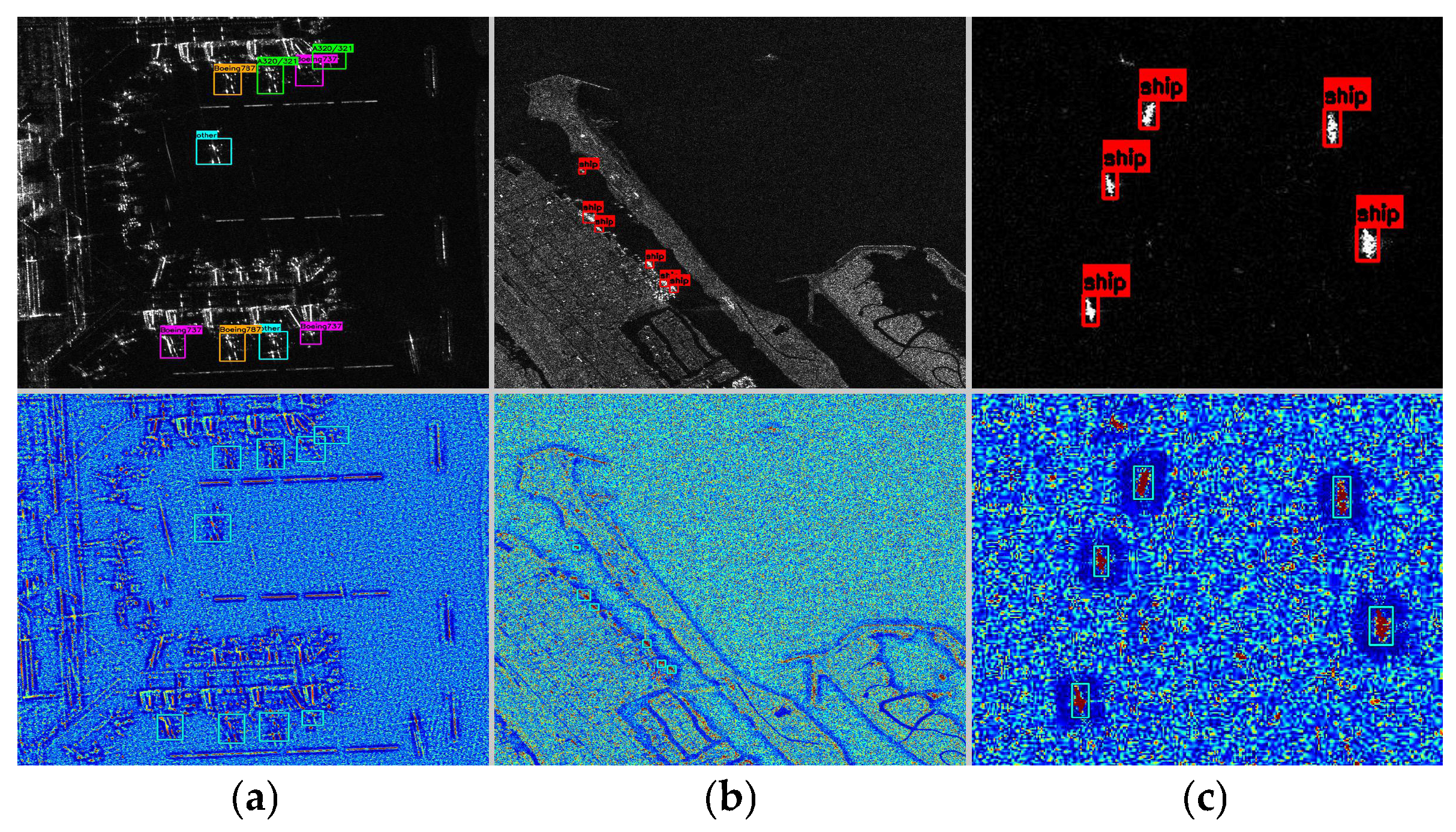
Despite these advances, the performance of deep SAR detectors is often influenced by the compatibility between network architecture and dataset characteristics. In real cases, different datasets may exhibit substantial variations in target–background separability, target density, scene structure, and clutter distribution. As shown in Figure 1, representative images from the SAR-Aircraft-1.0 [21], High-Resolution SAR Images Dataset (HRSID) [22], and SAR Ship Detection Dataset (SSDD) [23] datasets are presented. The first row shows the original images with ground-truth bounding boxes, while the second row shows the corresponding CFAR anomaly maps computed using Equation (5) in Section 3. These anomaly maps provide a visual indication of target–background separability in different SAR scenarios. Specifically, SAR-Aircraft-1.0 shows relatively low target–background separability due to structured airport backgrounds, HRSID exhibits an intermediate level of separability in more complex maritime scenes, and SSDD shows clearer separation under relatively homogeneous backgrounds. These observations suggest that a fixed network structure may not be equally suitable for SAR datasets with different target–background separability levels. Therefore, dataset characteristics should be considered when designing detection networks for diverse SAR scenarios.

To address model adaptability, existing approaches mainly follow two directions. The first seeks to improve cross-domain generalization through domain adaptation or domain generalization techniques [24,25,26,27], which attempt to align feature distributions across different datasets. The second relies on neural architecture search (NAS) to automatically explore optimal structures within predefined search spaces [28]. The former aims to develop a general-purpose model, whereas the latter focuses on discovering dataset-specific architectures. However, both directions exhibit some shortcomings. Domain adaptation typically requires target-domain data, domain generalization often requires assumptions about category-space alignment, and NAS entails substantial computational overhead and lacks interpretability.

In this work, a data-driven compromise model between general and specialized models is proposed. Inspired by the cell-averaging CFAR (CA-CFAR) principle [29], we first construct a CFAR anomaly response map and introduce a target–background separation margin to characterize the separability between annotated target regions and their surrounding contextual backgrounds. Based on this cue, a You Only Look Once version 8 (YOLOv8)-based SAR target detection network with three feature-fusion modes is developed. The overall detection framework remains consistent across datasets, while the feature-fusion structure is selected according to the CFAR-guided target–background separability of each dataset. The primary contributions are summarized as follows:

(1)

A CA-CFAR-based guided target–background separation margin is introduced to characterize target–background ambiguity in the CFAR anomaly response space. Instead of using CFAR as a standalone detector, the proposed criterion compares the average CFAR anomaly responses of target regions and their surrounding contextual backgrounds, thereby providing an interpretable cue for dataset-level mode selection.

(2)

A mode-selective SAR target detection framework based on YOLOv8 is developed. The framework consists of a lightweight representation-enhanced backbone, a mode-selective neck (MSN), and a complete intersection over the union modulated head (CMH). The backbone integrates ResNet18 and a dilated convolution spatial pyramid (DCSP) module to enhance contextual representation. The MSN contains three feature-fusion modes, namely deep, medium, and shallow modes, which are designed to match SAR datasets with different CFAR target–background separability levels. The CMH improves classification-regression alignment and suppresses clutter-induced responses.

(3)

Experiments are conducted on three public SAR target detection datasets, including SAR-Aircraft-1.0, HRSID, and SSDD. The experimental results demonstrate that matching the feature-fusion mode with dataset-level target–background separability improves detection performance. Moreover, the proposed CFAR-guided mode-selective network (CGMSN) achieves superior performance over several representative detectors on the evaluated datasets.

2. Related Work

2.1. CFAR-Based SAR Target Detection

The CFAR represents a classical adaptive detection framework based on local background statistical modeling and threshold-based decision-making. By estimating clutter statistics within sliding reference windows and determining the detection threshold based on a predefined false-alarm rate, CFAR maintains stable false-alarm control under varying clutter power. However, its performance inherently relies on two critical assumptions: local background homogeneity and the absence of contamination from targets or outliers [30]. When these assumptions are violated in heterogeneous scenes, both false alarms and missed detections increase significantly.

To address heterogeneous backgrounds, prior studies have primarily focused on improving the robustness of background estimation. Robust statistical CFAR variants employed truncated or censored samples and redesigned parameter estimation strategies to mitigate interference [2]. Region- or superpixel-based CFAR schemes replaced pixel-wise sliding windows with homogeneous spatial units obtained through segmentation, thereby enhancing background purity and reducing estimation variance [31]. These improvements suggested that CFAR performance enhancement was primarily achieved through refined clutter modeling rather than fundamentally new detection mechanisms.

Recently, CFAR has been extended toward system-level implementation and integration with learning-based frameworks. GPU-oriented implementations reformulated classical CFAR operations into parallel tensor-based computations to support large-scale and real-time SAR processing [32]. In addition, CFAR-guided deep learning approaches exploited CFAR outputs as interpretable priors or proposal generators in complex scenarios [33]. Unlike these approaches, this work does not use CFAR as the detector. Instead, CFAR is used to construct an anomaly response map, from which a target–background separation margin is derived as an interpretable cue for dataset-level mode selection.

2.2. Objects in SAR Target Detection

Existing SAR target detection studies have mainly focused on aircraft and ships, whereas other target categories have received relatively limited attention. Most deep learning-based methods have been developed for specific target categories. Accordingly, studies on aircraft and ship detection have primarily addressed the challenges encountered in their respective detection scenarios.

For aircraft detection, the main challenges include discrete strong scattering, structural discontinuities, incomplete contours, scale variations, complex background clutter, airport-dependent spatial distributions, and fine-grained category ambiguity. To address structural fragmentation, scattering-point- and scattering-region-based models have been developed to restore structural integrity [34,35,36,37]. To improve scale robustness, multi-scale feature extraction and fusion, together with a reformulation of the detection framework, have been adopted [38,39]. To suppress complex background clutter and speckle interference in airport scenes, saliency cues and contextual information have been incorporated to enhance target–background discrimination [35,37,39]. In addition, geospatial priors and probabilistic constraints have been utilized to characterize the aircraft–airport relationship for airport-aware detection [40]. For fine-grained aircraft detection, global structural cues and category relationship constraints have been introduced to improve discrimination performance [40].

For ship detection, the main challenges include small targets and weak scattering, scale variation, dense adjacency, arbitrary orientations, complex inshore clutter, speckle noise, and cross-domain shift. To address these issues, multi-scale feature extraction and fusion, shallow-detail enhancement, and detection head optimization have been introduced to improve small-target sensitivity and scale robustness [13]; anchor-free, key-point-based, and query-based detection methods have been adopted to alleviate target confusion in densely distributed scenes [10,13]; oriented bounding box representation and geometry-aware optimization have been developed to better characterize arbitrary orientations and elongated structures [15,16,20]; contextual information and attention mechanisms have been incorporated to suppress background clutters in complex inshore environments [15,17,19]; and feature alignment and domain adaptation have been explored to improve generalization across SAR datasets [24,25,26].

In fact, aircraft and ship detection exhibit both common and category-specific characteristics. The common challenges include multi-scale variation, speckle noise, background clutter, and target–background ambiguity. The category-specific challenges are mainly related to differences in scattering patterns, structural characteristics, and scene priors. Therefore, an effective SAR target detection framework should retain sufficient shared representation capability for generic SAR target modeling while also providing dataset-specific flexibility for different scene characteristics. To this end, we propose a mode-selective network for SAR target detection.

3. Method

3.1. Overall Framework

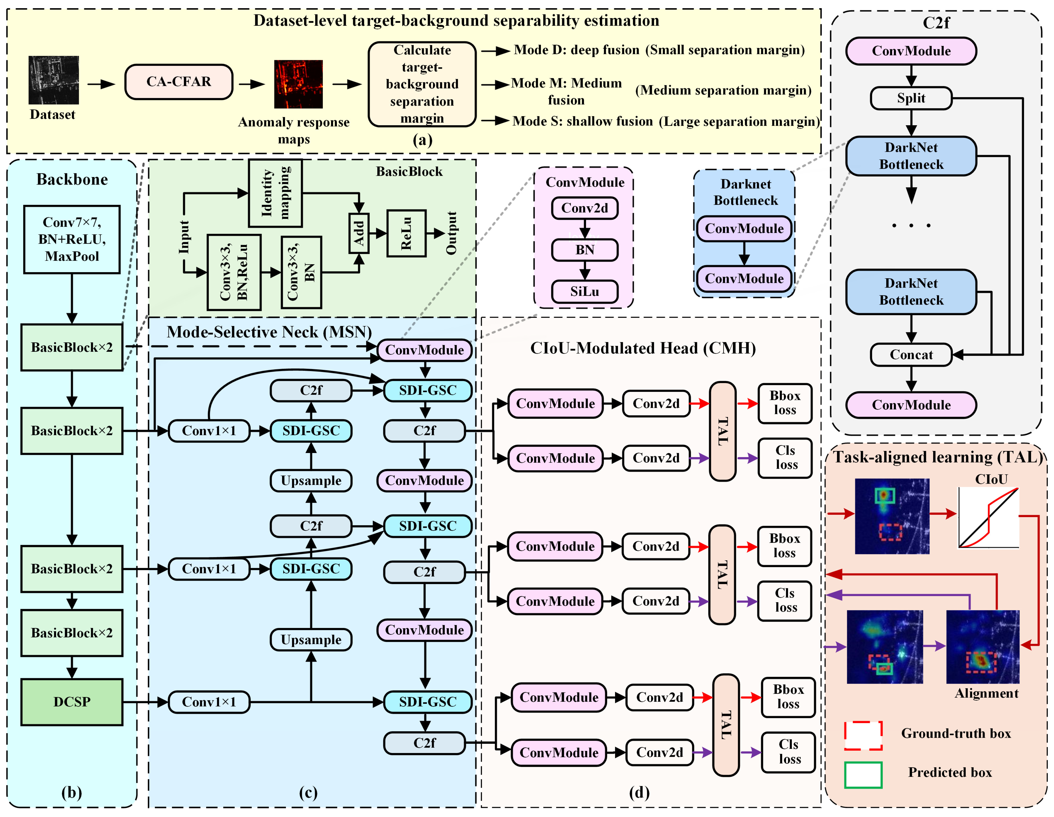
The overall framework of CGMSN is illustrated in Figure 2. It consists of two stages: CA-CFAR-guided target–background separability estimation and mode-selective SAR target detection. In the first stage, a CA-CFAR anomaly response map is constructed for each image, and a dataset-level target–background separation margin is calculated to characterize the separability between annotated target regions and their surrounding contextual backgrounds in the CFAR anomaly response space. This margin provides a training-free and interpretable cue for selecting the feature-fusion mode in the subsequent target detection. In the second stage, a YOLOv8-based mode-selective detector is constructed for SAR target detection. The detector consists of three major components: a lightweight representation-enhanced backbone for feature extraction, an MSN for multi-scale feature fusion, and a CMH for reliability-aware classification-regression alignment. Within the MSN, one feature-fusion mode is selected from three predefined modes according to the dataset-level target–background separation margin. The following subsections provide detailed descriptions of the CA-CFAR-guided separation margin calculation, backbone, MSN, and CMH.

3.2. A CA-CFAR-Based Target–Background Separability Estimation

To characterize the target–background separability of different SAR datasets, a CA-CFAR-based separability estimation is adopted. Following the classical CA-CFAR detection principle, local background statistics are estimated from the reference cells surrounding the cell under test (CUT). However, unlike conventional CFAR detection, this work uses CFAR as an interpretable statistical tool to construct a pixel-wise anomaly response map. For each pixel, the local background response is estimated from its surrounding reference region while excluding the guard region. The normalized local response is then converted into a CFAR anomaly response, where a larger value indicates that the pixel is more distinct from its surrounding local background. Based on the anomaly response map, the target–background separation margin is calculated by comparing the average anomaly response inside annotated target regions with that of their surrounding contextual background regions. This margin directly reflects whether targets can be distinguished from their local backgrounds in the CFAR anomaly response space.

Suppose that a SAR image has a size of W × H, where W and H denote the width and height, respectively. For a CUT located at position (w, h) ($1\le w\le W$ and $1\le h\le H$), a two-dimensional sliding window is defined and divided into three regions: the CUT, guard cells, and reference cells. The CUT is located at the center of the window. The guard cells surround the CUT to prevent target energy leakage from contaminating the background estimation, while the reference cells are located outside the guard region and are assumed to mainly contain pure background clutter.

Let M denote the total number of reference cells. The local average clutter power $Z\left(w, h\right)$ around the CUT is computed as

$$Z\left(w, h\right)={\displaystyle \frac{1}{M}}{\displaystyle \sum _{m=1}^M{X}_m}$$

(1)

where $X_m$ denotes the amplitude value of the m-th (m = 1, 2, …, M) reference cell.

Based on the estimated local clutter power, the normalized CFAR response of the CUT is defined as

$$R\left(w,h\right)={\displaystyle \frac{X\left(w, h\right)}{Z\left(w, h\right)}}$$

(2)

where $X\left(w, h\right)$ denotes the amplitude value of the CUT.

Under the classical CA-CFAR assumption, if the CUT and the reference cells follow the same homogeneous clutter distribution, the probability that a background cell produces a normalized response larger than $R\left(w, h\right)$ can be written as

$$p\left(w, h\right)={\left(1+{\displaystyle \frac{R(w, h)}{M}}\right)}^{-M}$$

(3)

A smaller $p\left(w, h\right)$ means that the current response is less likely to be generated by homogeneous background clutter. Accordingly, the pixel-wise CFAR anomaly response is defined as

$$A\left(w, h\right)=-\log p\left(w, h\right)$$

(4)

Substituting (3) into (4), the anomaly response can be obtained as

$$A\left(w, h\right)=M\log \left(1+{\displaystyle \frac{R\left(w, h\right)}{M}}\right)=M\log \left(1+{\displaystyle \frac{X\left(w, h\right)}{M\left[Z\left(w, h\right)\right]}}\right)$$

(5)

The resulting anomaly response map provides a continuous CFAR-based description of local abnormality. Pixels with larger anomaly responses are more distinct from their surrounding reference background. Different from conventional CFAR detection, this work uses the anomaly response map to evaluate the separability between annotated target regions and their surrounding contextual backgrounds.

Suppose one dataset contains $N_D$ images, and the j-th (j = 1, 2, …$N_D$) image includes $N_j$ targets. For the i-th (i = 1, 2, … $N_j$) target, we calculate the average anomaly degree within the target region ${\Omega }_{i,j}^t$ as

$${\mu }_{i,j}^t={\displaystyle \frac{1}{\left|{\Omega }_{i,j}^t\right|}}{\displaystyle \sum _{\left(w,h\right)\in {\Omega }_{i,j}^t}A\left(w, h\right)}.$$

(6)

Next, expand the target region to obtain a surrounding region ${\Omega }_{i,j}^{ext}$ and define the context region ${\Omega }_{i,j}^{ctx}={\Omega }_{i,j}^{ext}\backslash {\Omega }_{i,j}^t$ by excluding the target itself. The average anomaly degree of this context region is then calculated as

$${\mu }_{i,j}^{ctx}={\displaystyle \frac{1}{\left|{\Omega }_{i,j}^{ctx}\right|}}{\displaystyle \sum _{\left(w,h\right)\in {\Omega }_{i,j}^{ctx}}A\left(w, h\right)}$$

(7)

Finally, we define the target–background CFAR separation margin as the average difference between target and context anomaly degrees across the entire dataset as follows:

$${\Delta }_{tb}^D={\displaystyle \frac{1}{N_D}}{\displaystyle \sum _{j=1}^{N_D}\left(\frac{1}{N_j}{\displaystyle \sum _{i=1}^{N_j}\left({\mu }_{i,j}^t-{\mu }_{i,j}^{ctx}\right)}\right)}$$

(8)

A smaller ${\Delta }_{tb}^D$ indicates that the local anomaly responses of target regions and surrounding backgrounds have similar local anomaly responses, implying stronger target–background ambiguity. Conversely, a larger ${\Delta }_{tb}^D$ corresponds to higher separability.

3.3. Lightweight Representation-Enhanced Backbone

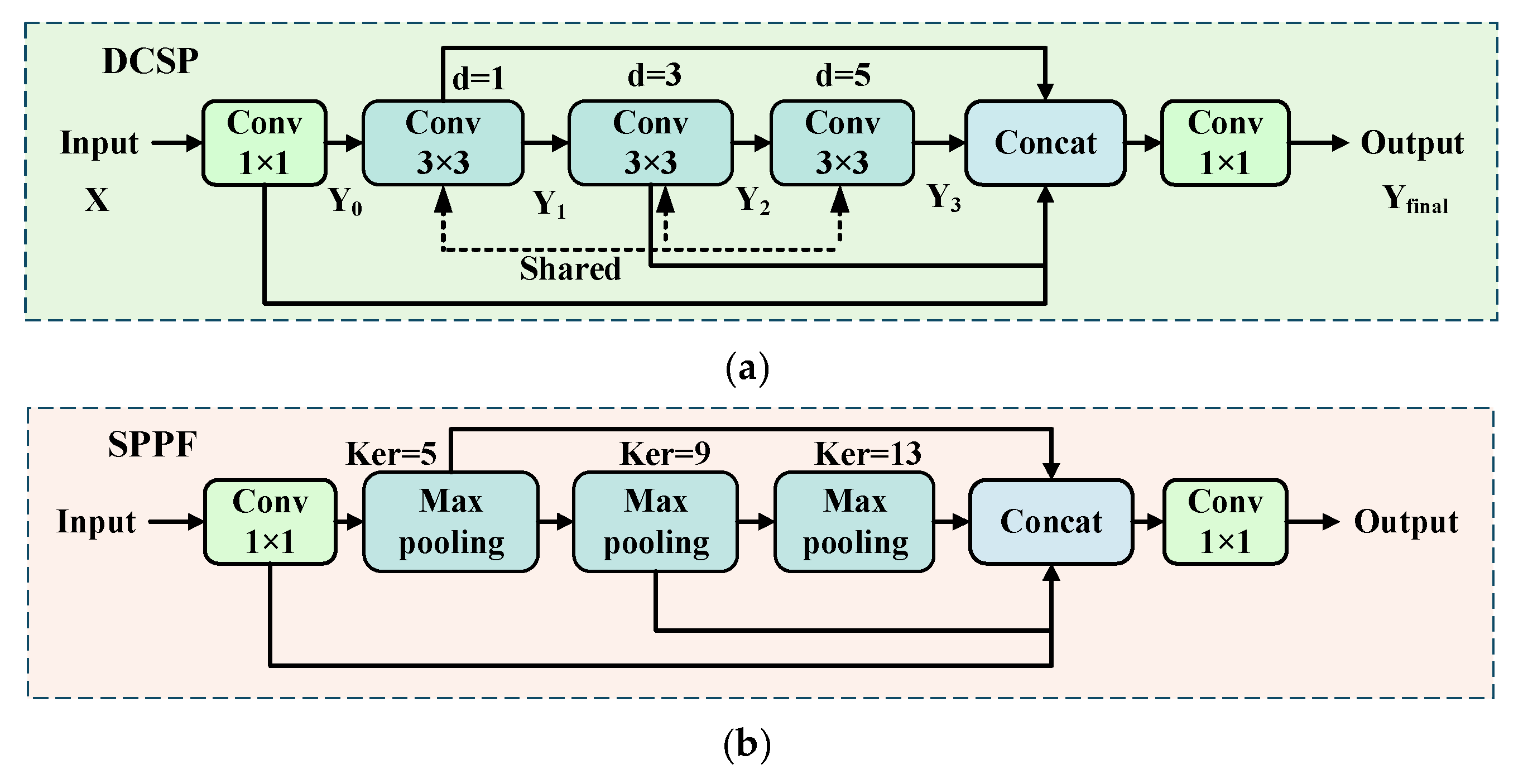
A lightweight backbone integrating ResNet18 with a DCSP module is adopted for feature extraction. ResNet18 is selected for its moderate depth and stable optimization behavior, which are well-suited to SAR datasets with limited training samples. Compared with deeper architectures, it alleviates the risk of overfitting while preserving its representation capacity. In addition, the DCSP module, derived from the original spatial pyramid pooling-fast (SPPF) module in YOLOv8, is integrated into the backbone to enhance contextual perception without introducing excessive parameters. Unlike SPPF, which enlarges the receptive field through fixed pooling operations, DCSP employs cascaded dilated convolutions with shared weights to achieve learnable receptive-field expansion.

The detailed structures of DCSP and SPPF are shown in Figure 3a,b, respectively. The DCSP module applies a standard 1 × 1 convolution to reorganize channel information, followed by three cascaded 3 × 3 dilated convolution operations with different dilation rates. The intermediate feature maps can be expressed as

$$\left\{\begin{array}{l}{Y}_0=Con{v}_{1\times 1}\left(X\right)\hfill \\ Y_1=Con{v}_{3\times 3}^{d=1}\left(Y_0, W_{share}\right)\hfill \\ Y_2=Con{v}_{3\times 3}^{d=3}\left(Y_1, W_{share}\right)\hfill \\ Y_3=Con{v}_{3\times 3}^{d=5}\left(Y_2, W_{share}\right)\hfill \end{array}\right.$$

(9)

where $X$ denotes the input feature maps, $Conv\left(\cdot \right)$ represents a convolution operation, d is the dilation rate, and $W_{share}$ denotes the shared convolution parameters across the cascaded layers.

The final output of DCSP can be expressed by,

$$Y_{final}=Con{v}_{1\times 1}\left(Concat\left(Y_0, Y_1, Y_2, Y_3\right)\right)$$

(10)

where $Concat\left(\cdot \right)$ denotes channel-wise concatenation.

The DCSP design provides two primary advantages. First, progressive dilation enlarges the effective receptive field in a learnable, hierarchical manner, which is beneficial for modeling anisotropic scattering patterns and contextual dependencies in SAR imagery. Second, weight sharing across the dilated convolutions reduces parameter redundancy and introduces implicit regularization, encouraging scale-consistent feature learning while maintaining computational efficiency.

3.4. Mode-Selective Neck

To align the feature-fusion depth with the CFAR-guided target–background separability of different datasets, an MSN is designed for feature fusion. In the original YOLOv8, the feature pyramid network and path aggregation network (FPN-PAN) adopt fixed multi-scale fusion pathways, where the feature interaction pattern remains unchanged across different SAR scenarios. However, SAR datasets may exhibit different levels of target–background separability in the CFAR anomaly response space. Therefore, a fixed fusion mode may be suboptimal for all datasets with different separability characteristics.

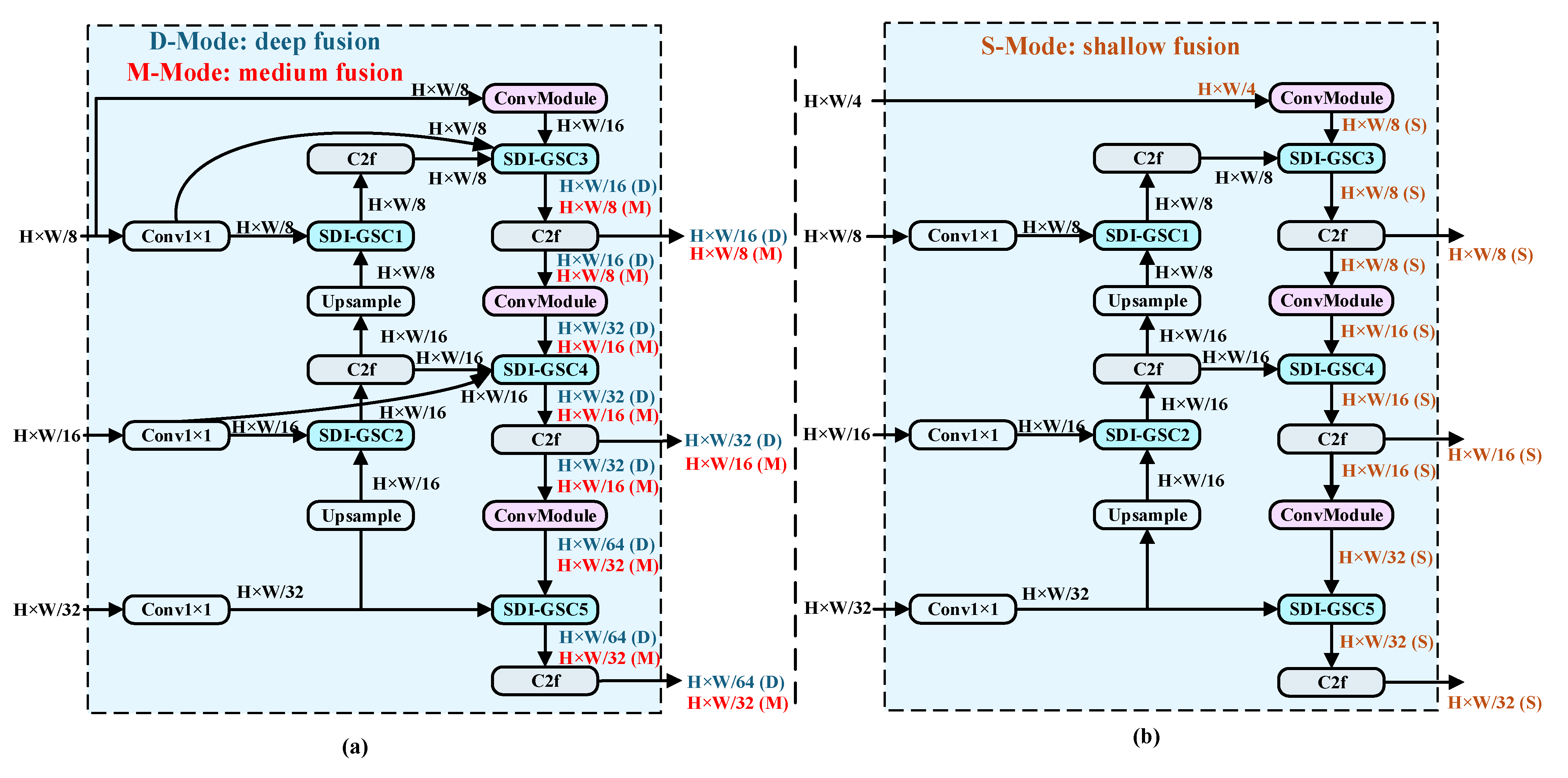
For datasets with smaller CFAR target–background separation margins, targets are more easily confused with surrounding backgrounds, and deeper cross-scale feature fusion is expected to enhance contextual representation and target–background discrimination. In contrast, for datasets with larger separation margins, targets are more distinguishable from their surrounding backgrounds, and shallower fusion can be sufficient while reducing unnecessary feature aggregation. Based on this consideration, MSN provides three predefined feature-fusion modes to match SAR scenarios with different target–background separability levels, as shown in Figure 4.

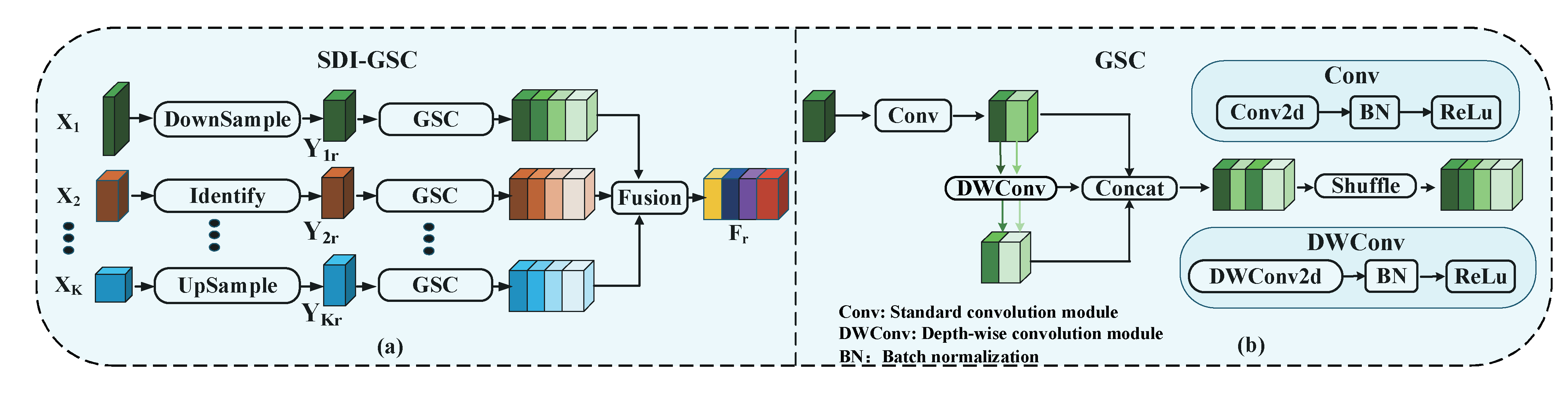
As shown in Figure 4, inspired by the multi-scale fusion principle of bidirectional FPN (BiFPN), both the deep feature-fusion mode (D-Mode) and the medium feature-fusion mode (M-Mode) adopt multi-path feature aggregation, whereas the shallow feature-fusion mode (S-Mode) performs two-path feature aggregation. The basic fusion unit adopted in these three modes is designed by integrating semantic and detail infusion (SDI) [41] and grouped shuffle convolution (GSC) [42], aiming to enhance both feature representation and inter-channel information exchange. The structure of SDI-GSC is shown in Figure 5a. Before fusion, feature maps from different paths are transformed to a unified spatial resolution through up-sampling, identity mapping, or down-sampling operations when necessary. In D-Mode and M-Mode, SDI-GSC receives feature inputs from multiple paths, enabling denser feature aggregation and stronger feature interaction. In contrast, S-Mode restricts each SDI-GSC unit to two same-scale feature branches, resulting in a shallower and more lightweight fusion structure.

Suppose that the features to be fused come from K branches. The feature map from the k-th (k = 1, 2, …, K) branch is denoted as $X_k$. To fuse features at a specific target scale, all input features are first aligned to the spatial resolution of the r-th ($1\le r\le K$) branch, denoted as $X_r$. The transformed feature map of the k-th branch can then be expressed as

$$Y_{kr}=\left\{\begin{array}{ll}U\left(X_k\right),\hfill & \mathcal{S}\left(X_k\right)<\mathcal{S}\left(X_r\right)\hfill \\ I\left(X_k\right),\hfill & \mathcal{S}\left(X_k\right)=\mathcal{S}\left(X_r\right)\hfill \\ D\left(X_k\right),\hfill & \mathcal{S}\left(X_k\right)>\mathcal{S}\left(X_r\right)\hfill \end{array}\right.$$

(11)

where $\mathcal{S}\left(\cdot \right)$ represents the spatial resolution of feature map $X$; $D\left(\cdot \right)$ represents a down-sampling operation; $I\left(\cdot \right)$ represents an identity mapping operation; and $U\left(\cdot \right)$ represents an up-sampling operation.

After scale alignment, GSC is employed to enhance inter-channel information exchange, as shown in Figure 5b. It combines standard convolution and depth-wise convolution to extract complementary feature representations with moderate computational cost. A channel shuffle operation is then applied to promote cross-channel information interaction. This design improves parameter efficiency while preserving effective representation. Given the aligned feature $Y_{kr}$, the output of GSC is formulated as

$$F_{kr}=Shuffle\left(Concat\left(Conv\left(Y_{kr}\right), DWConv\left(Conv\left(Y_{kr}\right)\right)\right)\right)$$

(12)

where $Conv\left(\cdot \right)$ represents standard convolution; $DWConv\left(\cdot \right)$ represents depth-wise convolution; and $Shuffle\left(\cdot \right)$ represents the channel shuffling operation.

Finally, for D-Mode and M-Mode, the enhanced feature maps from different branches are fused through Hadamard multiplication. The multiplicative interaction emphasizes mutually consistent activations across different feature branches and suppresses inconsistent responses, which is helpful for reducing background-induced false responses in SAR scenes with strong target–background ambiguity. Given the GSC-enhanced features ${\left\{F_{kr}\right\}}_{k=1}^K$ aligned to the r-th scale, the output feature can be expressed as

$$F_r=F_{1r}\odot F_{2r}\odot \dots \odot F_{Kr}$$

(13)

where $\odot$ denotes the Hadamard product.

For S-Mode, the enhanced features from the two paths are fused by concatenation following the original YOLOv8 paradigm. This design avoids unnecessary deep aggregation and helps preserve local discriminative details for datasets with clearer target–background separation.

3.5. CIoU-Modulated Head

YOLOv8 adopts an anchor-free detection paradigm, in which each spatial prediction location on the feature map directly outputs classification scores and bounding box regression parameters. In its detection head, a task-aligned learning (TAL) mechanism is employed to couple classification confidence with localization accuracy. Specifically, an alignment metric—typically formulated as the product of classification probability and complete intersection over union (CIoU) —is used to jointly represent category confidence and regression quality. However, in SAR target detection, targets such as aircraft and ships are frequently embedded in strong and heterogeneous background clutter. This clutter seriously perturbs the CIoU calculation of predicted bounding boxes, leading to compressed CIoU distributions and reduced separability between high-quality and low-quality predictions. As a result, the alignment metric becomes less discriminative, weakening the reliability of positive sample selection.

To mitigate this issue, a CMH is proposed, as illustrated in Figure 2. The core idea is to reshape the CIoU distribution before task-aligned computation by amplifying reliable predictions and suppressing clutter-induced unreliable ones. By incorporating this CIoU modulation into the TAL module, the dynamic range of localization quality is enlarged, thereby improving the robustness of alignment-based sample assignment. Let the batch size be B, the number of ground-truth targets in each image be J, and the total number of prediction locations be N. For the n-th prediction location (n = 1, 2, …, N) in the b-th (b = 1, 2, …, B) image, the classification head outputs a raw score $S_{bn}^{raw}$, and the regression head predicts location distributions $D_{bn}^{pred}$. After applying the sigmoid function, the classification probability is obtained as $S_{bn}^{prob}$. The regression outputs are decoded into predicted bounding boxes $B_{bn}^{pred}$.

For the j-th (j = 1, 2, …, J) ground-truth box $B_{bj}^{gt}$ in the b-th image, the CIoU between $B_{bn}^{pred}$ and $B_{bj}^{gt}$ is computed as

$$I_{bjn}=\mathrm{C}\mathrm{I}\mathrm{o}\mathrm{U}\left(B_{bn}^{Pred}, B_{bj}^{gt}\right)$$

(14)

During the task alignment, the CIoU is nonlinearly modulated to expand the separability between reliable and unreliable predictions as follows:

$${I^{\prime }}_{bjn}=\left\{\begin{array}{cc}{\left(I_{bjn}\right)}^{1/Power},& I_{bjn}\ge I_0\\ {\left(I_{bjn}\right)}^{Powe{r}^2},& I_{bjn}<I_0\end{array}\right.$$

(15)

where $I_0$ represents the threshold, and $Power=2$.

This modulation increases the contrast between high-CIoU and low-CIoU samples. High-quality predictions receive amplified supervision signals, whereas clutter-induced low-overlap predictions are suppressed. From an optimization perspective, this reshaping redistributes gradient contributions toward reliable candidates.

The probability that the n-th prediction location belongs to the category of the j-th ground-truth target is defined as

$$S_{bjn}=S_{bn{L}_{bj}}^{prob}$$

(16)

where $L_{bj}$ represents the category label of the j-th ground-truth box in the b-th image.

The alignment metric is computed by jointly considering classification probability and modulated CIoU as follows:

$$A_{bjn}={\left(S_{bjn}\right)}^{\alpha }\times {\left({I^{\prime }}_{bjn}\right)}^{\beta }$$

(17)

where $\alpha =1$ and $\beta =6$.

For each ground-truth target, only prediction locations with high alignment scores are retained as candidate positive samples, thereby improving computational efficiency while restricting supervision to geometrically plausible locations. Specifically, for the j-th ground-truth target, select the top K predictions ranked by $A_{bjn}$ as candidate samples by using the mask $M_{bjn}^{topK}$. Additionally, spatial constraints are enforced so that only predictions located inside the ground-truth box are retained via mask $M_{bjn}^{in}$.

The positive sample mask of the j-th ground-truth target is defined as

$$M_{bjn}^{pos,initial}=M_{bjn}^{topK}\times M_{bjn}^{in}.$$

(18)

To avoid assigning multiple targets to the same prediction location, conflict resolution is performed. For the n-th prediction location, if it is assigned to multiple ground-truth targets, only the one with the maximum CIoU is retained.

$$M_{bjn}^{pos}=\left\{\begin{array}{cc}1,\hfill & if\hspace{0.17em}j=\underset{j\in J_{bn}^{initial}}{\mathrm{argmax}}{I}_{bjn}\\ 0,\hfill & otherwise\end{array}\right.$$

(19)

where $J_{bn}^{initial}=\left\{j\left|M_{bjn}^{pos,initial}=1\right.\right\}$ represents an index set of ground-truth targets assigned to the n-th prediction location in the b-th image.

The alignment metric is then filtered using the final mask $M_{bjn}^{pos}$ as follows:

$$A_{bjn}^{filtered}=A_{bjn}\times M_{bjn}^{pos}.$$

(20)

To stabilize training by preventing domination from extreme alignment values, the relative quality score of the n-th prediction location for the j-th ground-truth target is defined as

$$Q_{bjn}={\displaystyle \frac{A_{bjn}^{filtered}\times I_{bj}^{\max }}{A_{bj}^{\max }}}$$

(21)

where $A_{bj}^{\max }$ and $I_{bj}^{\max }$ can be calculated by

$$\left\{\begin{array}{c}{A}_{bj}^{\max }=\underset{n}{\max }{A}_{bjn}^{filtered}\\ I_{bj}^{\max }=\underset{n}{\max }\left({I^{\prime }}_{bjn}\times M_{bjn}^{pos}\right)\end{array}\right..$$

(22)

For each prediction location n in the b-th image, the final quality weight is determined by taking the maximum relative quality score across all ground-truth targets assigned to the location.

$$W_{bn}=\underset{j}{\max }{Q}_{bjn}.$$

(23)

3.6. Loss Function

In the anchor-free YOLOv8 framework, each prediction location outputs classification scores and bounding box regression distributions. Therefore, ground-truth labels must be reformulated into target representations aligned with prediction locations.

For each prediction location n in the b-th image selected as positive samples after task-aligned selection, the corresponding target category label and bounding box are assigned as

$$\left\{\begin{array}{c}{L}_{bn}^{target}=L_{b,J_{bn}}^{gt}\\ B_{bn}^{target}=B_{b,J_{bn}}^{gt}\end{array}\right.$$

(24)

where $J_{bn}=\left\{j\left|M_{bjn}^{pos}=1\right.\right\}$.

Classification Loss: Instead of using a hard binary label, the soft-weighting mechanism allows high-quality positive samples to contribute more to optimization. The soft category label is obtained by weighing the target category label with the final quality weight from task alignment, which can be expressed as

$$L_{bn}=L_{bn}^{target}\times W_{bn}.$$

(25)

With this soft label, the classification loss is formulated using binary cross-entropy:

$${\mathcal{L}}_{cls}={\displaystyle \frac{-{\displaystyle \sum _{b=1}^B{\displaystyle \sum _{n=1}^N\left[L_{bn}\log \left(S_{bn}^{pred}\right)+\left(1-L_{bn}\right)\log \left(1-S_{bn}^{pred}\right)\right]}}}{{\displaystyle \sum _{b=1}^B{\displaystyle \sum _{n=1}^N{W}_{bn}}}}}.$$

(26)

Regression Loss: Let $fg=\left\{\left(b,n\right)\left|\exists j\hspace{0.17em}s.t.\hspace{0.17em}{M}_{bjn}^{pos}=1\right.\right\}$ denote the set of prediction locations assigned to at least one ground-truth box. The regression loss can be written as

$${\mathcal{L}}_{reg}={\displaystyle \frac{{\displaystyle \sum _{\left(b,n\right)\in fg}{W}_{bn}\cdot \left[1-\mathrm{C}\mathrm{I}\mathrm{o}\mathrm{U}\left(B_{bn}^{pred},B_{bn}^{target}\right)\right]}}{{\displaystyle \sum _{b=1}^B{\displaystyle \sum _{n=1}^N{W}_{bn}}}}}.$$

(27)

Distribution Focal Loss (DFL): YOLOv8 adopts DFL to model bounding box offsets as discrete probability distributions. For the l-th coordinate at prediction location n (where $l\in \left\{left,top,right,bottom\right\}$ indexes the box edge), the predicted distribution $d_t^{bnl}$ is converted to a probability distribution via softmax as follows:

$$p_t^{bnl}={\displaystyle \frac{\exp \left(d_t^{bnl}\right)}{{\displaystyle \sum _{t^{\prime }=0}^{Regmax-1}\exp \left(d_{t^{\prime }}^{bnl}\right)}}},\hspace{1em}t=0,1,\dots ,Regmax-1$$

(28)

where $Regmax$ is the maximum regression bin index.

For the target distribution $y^{bnl}$ encoded from $B_{bn}^{target}$, the left and right bin indices and the corresponding interpolation weights are defined as

$$\left\{\begin{array}{c}{t}_{left}=⌊y^{bnl}⌋\\ t_{right}=t_{left}+1\\ W_{left}=t_{right}-y^{bnl}\\ W_{right}=1-W_{left}\end{array}\right.$$

(29)

where $⌊\cdot ⌋$ represents the floor operation.

The DFL is computed as

$${\mathcal{L}}_{dfl}={\displaystyle \frac{{\displaystyle \sum _{\left(b,n\right)\in fg}{W}_{bn}\left[{\displaystyle \sum _{l=1}^4{\mathcal{L}}_{dfl}^0\left(p^{bnl},y^{bnl}\right)}\right]}}{{\displaystyle \sum _{b=1}^B{\displaystyle \sum _{n=1}^N{W}_{bn}}}}}$$

(30)

where

$${\mathcal{L}}_{dfl}^0\left(p^{bnl},y^{bnl}\right)=-\left[W_{left}\cdot \log \left(p_{t_{left}}\right)+W_{right}\log \left(p_{t_{right}}\right)\right].$$

(31)

Finally, the total loss can be expressed by

$${\mathcal{L}}_{total}={\lambda }_{cls}{\mathcal{L}}_{cls}+{\lambda }_{reg}{\mathcal{L}}_{reg}+{\lambda }_{dfl}{\mathcal{L}}_{dfl}$$

(32)

where ${\lambda }_{cls}$, ${\lambda }_{reg}$, and ${\lambda }_{dfl}$ are balancing coefficients.

It is worth noting that the proposed CIoU modulation influences both sample assignment and quality weight, thereby implicitly affecting the optimization of classification, regression, and DFL losses, as reflected in (26), (27), and (30), respectively.

4. Experiments

4.1. Datasets

Experiments are conducted on three representative public SAR target detection datasets with different target–background separability levels, namely SAR-Aircraft-1.0, HRSID, and SSDD.

SAR-Aircraft-1.0 consists of 4368 SAR images acquired by the GaoFen-3 satellite [21], containing 16,463 aircraft instances across seven fine-grained categories. There are Boeing 737, Boeing 787, A220, A320/321, A330, ARJ21, and other categories. This dataset is characterized by complex airport environments, dense target distribution, strong structural interference from airport facilities, multi-scale aircraft instances, and fine-grained classification requirements. Such characteristics result in strong background clutter and heterogeneous scattering patterns. The dataset is split into training, validation, and test sets with a 7:1:2 proportion.

HRSID contains 5604 SAR images collected from three satellites, with 16,951 ship instances [22]. Unlike SAR-Aircraft-1.0, it includes only a single ship category without fine-grained subdivision. Ships are distributed in offshore and nearshore scenes, accounting for 81.6% and 18.4%, respectively. Since most targets are located in offshore areas with relatively homogeneous backgrounds, the overall dataset complexity is relatively low. The dataset is split into training, validation, and test sets with an 8:1:1 ratio.

SSDD is a widely used public dataset for SAR ship detection. It contains 1160 SAR images acquired from RadarSat-2, TerraSAR-X, and Sentinel-1, containing a total of 2551 annotated ship instances [23]. Following the common data partitioning scheme used in related research, we divide the entire dataset into training and test sets in a 4:1 ratio.

4.2. Experimental Setup and Evaluation Metrics

All experiments are conducted on an NVIDIA GeForce RTX 4080 GPU with 16 GB of memory. The implementation is based on Python 3.10.14, PyTorch 2.2.2, and CUDA 12.1. The models are trained using the SGD optimizer with an initial learning rate of 0.01. The batch sizes for SAR-Aircraft-1.0, HRSID, and SSDD are set to 8, 32, and 4, respectively.

Model performance is evaluated from three perspectives: detection accuracy, model complexity, and computational efficiency [43]. Detection accuracy is assessed using precision (P), recall (R), and COCO-style metrics, including AP50, AP75, and AP50:95. Model complexity is assessed in terms of the number of parameters and floating-point operations (FLOPs). Computational efficiency is measured by the inference speed, reported in frames per second (FPS), measured on a single GPU.

4.3. CFAR-Guided Target–Background Separability Assessment

To quantitatively assess target–background separability at the dataset level, the proposed CA-CFAR-guided separation margin is calculated on SAR-Aircraft-1.0, HRSID, and SSDD. For each image, a CFAR anomaly response map is first computed according to (5). Then, for each annotated target, the average anomaly response inside the target region and that of its surrounding contextual background region are calculated. The image-level target–background separation margin is obtained by averaging the response differences over all targets in the image, and the dataset-level separation margin is further obtained by averaging over all images in the dataset as given by (8).

The results for the three datasets are presented in

Table 1. Target–background separability assessment.

Dataset	Target–Background Separation Margin	Separability Level	Selected Feature-Fusion Mode
SAR-Aircraft-1.0	0.0076	Low	D-Mode
HRSID	0.2018	Medium	M-Mode
SSDD	0.2616	High	S-Mode

. The dataset-level separation margins of SAR-Aircraft-1.0, HRSID, and SSDD are 0.0076, 0.2018, and 0.2616, respectively. SAR-Aircraft-1.0 achieves a small separation margin, indicating strong target–background ambiguity in the CFAR anomaly response space. Accordingly, D-Mode is chosen to realize deeper feature fusion. With an intermediate separation margin, HRSID is assigned to M-Mode for moderate feature aggregation. SSDD achieves a relatively high separation margin, enabling targets to be easily distinguished from the background. Therefore, S-Mode is adopted to achieve a shallow fusion structure. For a new dataset, the calculated separation margin can be compared with these three levels to select the closest feature-fusion mode.

4.4. Ablation Experiment

Ablation experiments are conducted on both SAR-Aircraft-1.0, HRSID, and SSDD with the original YOLOv8 serving as the baseline. To ensure fairness and mitigate the risk of overfitting due to limited SAR training data, ResNet18 is used as the backbone in the baseline, while the original FPN-PAN neck and detection head are retained. Based on this baseline, DCSP, MSN, and CMH are progressively incorporated to evaluate their respective effectiveness and complementary contributions.

Results on SAR-Aircraft-1.0: The ablation results are presented in

Table 2. Ablation experiments on SAR-Aircraft-1.0.

Baseline	DCSP	MSN	CMH	P (%)	R (%)	AP50 (%)	AP75 (%)	AP50:95 (%)	Parameters (M)	FLOPs (G)	FPS
√				85.5	90.5	93.8	80.5	70.6	17.9	46.3	285
√	√			85.9	91	94.5	80.7	71	18.5	46.3	278
√		√		86.8	92.5	95.3	81	70.9	14.3	35.8	251
√			√	88.4	92.6	96.4	81.3	71.3	17.9	46.3	286
√	√	√		87.6	93	95.1	80.9	71.4	14.9	35.8	250
√		√	√	89	92.5	95.8	81.4	71.9	14.3	35.8	253
√	√		√	87.3	94.1	96.6	80.8	71.5	18.5	46.3	279
√	√	√	√	89.3	94.3	96.7	81.5	72	14.9	35.8	253

Note: “√” denotes selected items.

. After introducing DCSP into the backbone, P, R, AP50, AP75, and AP50:95 are increased by 0.4%, 0.5%, 0.7%, 0.2%, and 0.4%, respectively. Meanwhile, the number of parameters shows a slight increase, while the inference speed exhibits a marginal decrease, indicating that DCSP enhances feature representation at a low additional cost. Replacing the original FPN-PAN with MSN improves P, R, AP50, AP75, and AP50:95 by 1.3%, 2%, 1.5%, 0.5%, and 0.3%, respectively. The notable gains in precision, recall, and AP50 suggest more efficient multi-scale feature aggregation and better prediction quality in complex airport scenes. In addition, MSN significantly reduces parameters and FLOPs. Although FPS decreases from 285 to 251, this is mainly due to the additional multi-branch fusion and feature alignment operations, which are less hardware-efficient despite their lower theoretical computational cost. Replacing the original detection head with CMH improves P, R, AP50, AP75, and AP50:95 by 2.9%, 2.1%, 2.6%, 0.8%, and 0.7%, respectively. The larger gains in precision, recall, and AP50 indicate that CMH mainly improves overall prediction quality by enhancing the alignment between classification confidence and localization reliability. Consequently, false alarms and missed detections are reduced, while parameters, FLOPs, and FPS remain nearly unchanged.

For the dual-module settings, DCSP + MSN further improves precision, recall, and AP50:95 over MSN alone, with only slight decreases in AP50 and AP75, indicating a trade-off between stronger feature representation and strict localization accuracy. MSN + CMH achieves clear gains in precision and AP50:95 over MSN alone, demonstrating effective complementarity between feature fusion and reliability-aware prediction modulation. DCSP + CMH yields the most notable gains in recall and AP50 compared with DCSP alone, suggesting improved target coverage and coarse-localization quality. The full model achieves the best performance, with P, R, AP50, AP75, and AP50:95 increased by 3.8%, 3.8%, 2.9%, 1%, and 1.4%, respectively, compared with the baseline. These results demonstrate that DCSP, MSN, and CMH can be effectively integrated to exploit complementary strengths and improve overall detection performance.

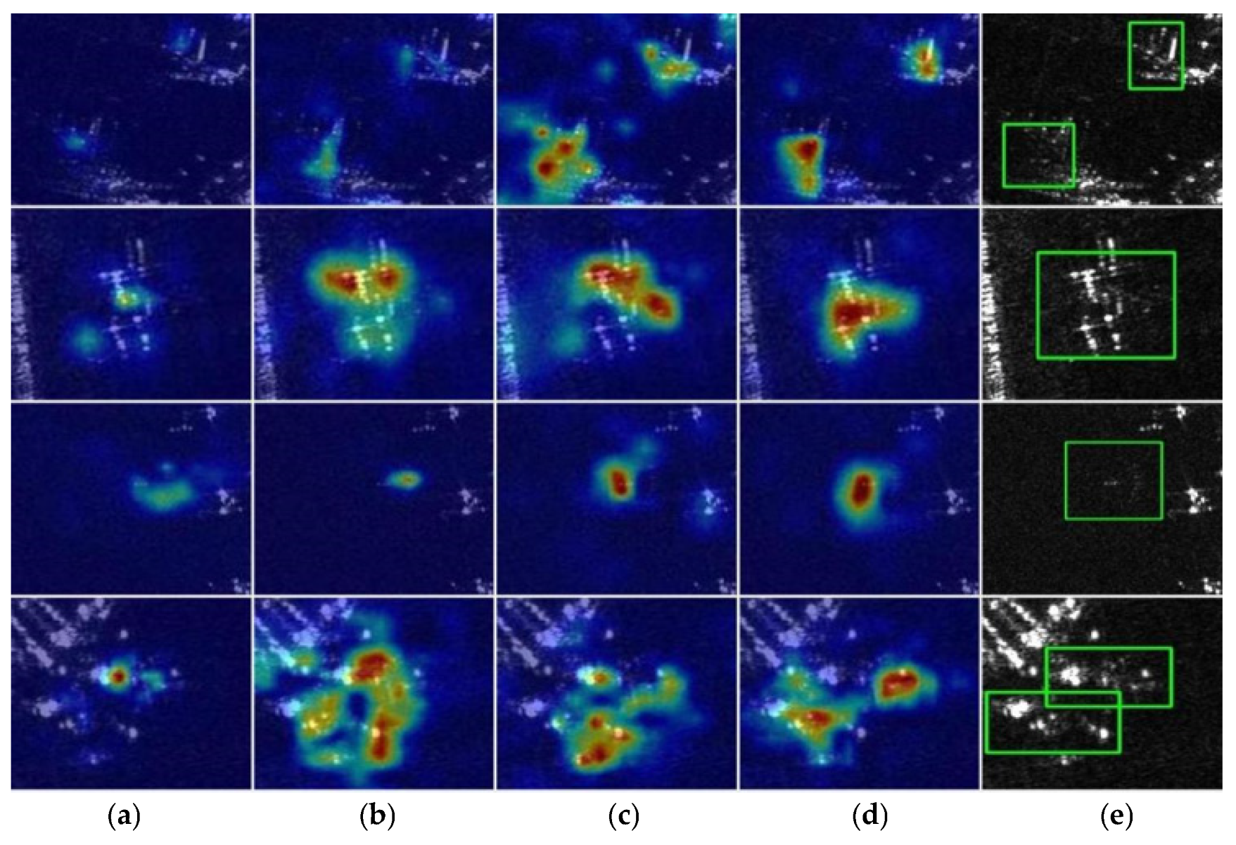
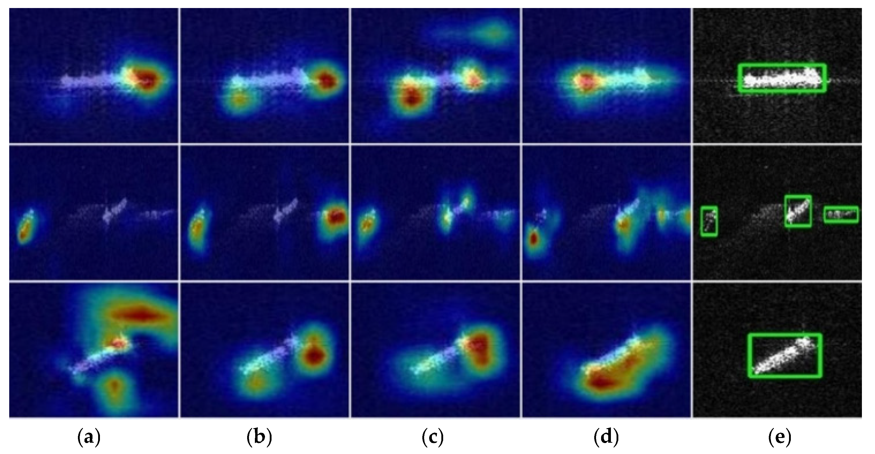
The heatmap visualizations of the baseline and the progressively enhanced variants on SAR-Aircraft-1.0 are presented in Figure 6. Specifically, the baseline is shown in Figure 6a, while Baseline + DCSP, Baseline + DCSP + MSN, and Baseline + DCSP + MSN + CMH are shown in Figure 6b–d, respectively. The ground truth is provided in Figure 6e. As shown in Figure 6a, the baseline fails to sufficiently highlight the targets’ weak-scattering components, resulting in incomplete activation across the target regions. After introducing DCSP into the backbone, as shown in Figure 6b, the activations become more concentrated around the dominant scattering centers, and the response intensity over the true target regions is noticeably enhanced. This improvement can be attributed to the enlarged receptive field and stronger contextual aggregation capability of DCSP. Nevertheless, some parts of the targets still exhibit relatively weak responses. In Figure 6c, after replacing the original FPN-PAN with MSN, the target regions are well activated, and the overall activation distribution becomes more spatially consistent due to enhanced cross-scale feature interaction and feature alignment. However, a few background regions show weak activations. After further replacing the original detection head with CMH, the heatmap in Figure 6d exhibits clearer target focus and sharper response boundaries. In particular, non-target strong scattering regions are significantly suppressed, and the activation responses are better aligned with the ground-truth bounding boxes in Figure 6e. These observations indicate that the proposed reliability-aware classification-regression alignment effectively mitigates clutter-induced false alarms and improves localization consistency within true target regions.

Results on HRSID: The ablation results are summarized in

Table 3. Ablation experiments on High-Resolution SAR Images Dataset (HRSID).

Baseline	DCSP	MSN	CMH	P (%)	R (%)	AP50 (%)	AP75 (%)	AP50:95 (%)	Parameters (M)	FLOPs (G)	FPS
√				90.9	85.7	91.5	79.8	69.4	17.9	46.3	243
√	√			92.2	85.6	92.2	79.9	70.5	18.5	46.3	233
√		√		93.2	84.2	92.2	80	70.4	14.3	43.2	219
√			√	91.6	85.9	92.5	79.7	70.2	17.9	46.3	239
√	√	√		92.9	86.4	93.2	80.7	71.1	14.9	43.2	210
√		√	√	92.5	85.9	92.7	80.6	70.9	14.3	43.2	211
√	√		√	92.6	86.6	91.6	81	70	18.5	46.3	232
√	√	√	√	93.6	87.4	93.3	81.2	71.9	14.9	43.2	211

Note: “√” denotes selected items.

. After introducing DCSP into the backbone, the gains in precision and AP50:95 are more pronounced than those observed on the SAR-Aircraft-1.0 dataset. Although recall decreases slightly by 0.1%, this can be regarded as a normal fluctuation. These results suggest that DCSP primarily improves target discrimination rather than recall on this dataset, since ship targets are set against relatively clean backgrounds, making target coverage less challenging. Replacing the original FPN-PAN with MSN yields clear improvements in precision and AP50:95, while recall decreases noticeably. This indicates that MSN effectively suppresses false alarms but tends to produce fewer positive predictions, leading to more precision-oriented behavior. Replacing the original detection head with CMH yields moderate overall improvements, while AP75 decreases slightly. This indicates that the benefit of CMH in relatively simple scenes is mainly reflected in overall prediction quality rather than further enhancement of high-CIoU localization.

For the dual-module settings, DCSP + MSN further improves all evaluation metrics over DCSP alone, demonstrating complementary effects between stronger feature representation and adaptive feature fusion. MSN + CMH improves recall over MSN alone, indicating that CMH can effectively alleviate the conservative prediction tendency introduced by MSN. DCSP + CMH yields a notable improvement in AP75 compared with CMH alone, suggesting that the combination is particularly beneficial for high-quality localization. The complete model yields consistent performance improvements across all evaluation metrics, demonstrating that the three proposed modules effectively complement one another. In addition, after introducing one or more modules, the variation trends of parameters, FLOPs, and FPS remain generally consistent with those on the SAR-Aircraft-1.0 dataset.

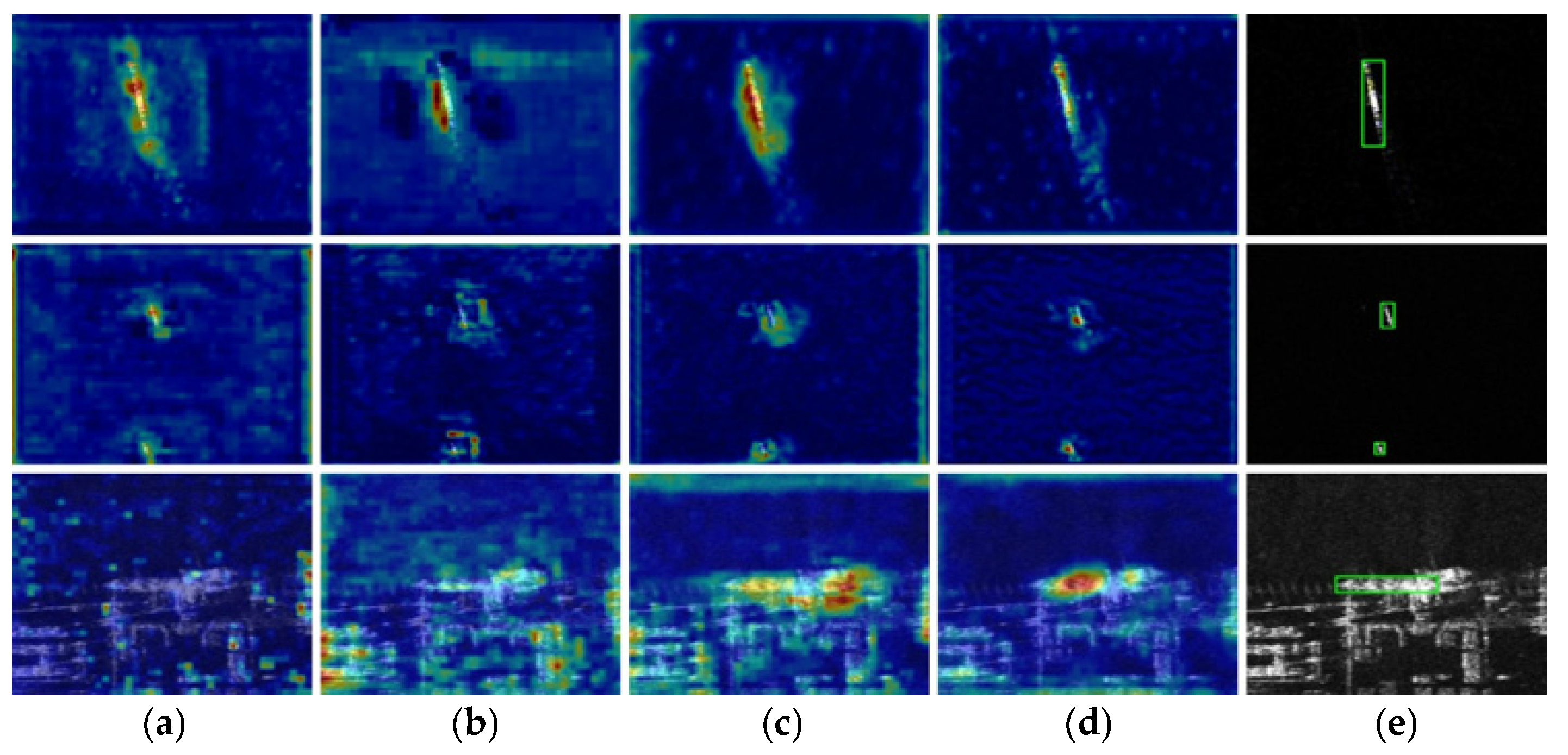
The heatmap visualizations of the baseline and its progressively enhanced variants on HRSID are presented in Figure 7. Specifically, the baseline is shown in Figure 7a, while Baseline + DCSP, Baseline + DCSP + MSN, and Baseline + DCSP + MSN + CMH are shown in Figure 7b–d, respectively. The ground truth is provided in Figure 7e. In Figure 7a, the phenomena where some target regions fail to be activated, and background clutter is activated and observed in different image samples. In Figure 7b, after introducing DCSP, the activation becomes more concentrated around the central target structure. However, some target regions still fail to be activated. In Figure 7c, after replacing the original FPN-PAN with MSN, all target regions are correctly activated, while some background regions are weakly activated. In Figure 7d, after further replacing the original detection head with CMH, the target regions are correctly activated, whereas the background clutter is not. Overall, Figure 7 verifies that each proposed component contributes progressively to improved target localization and clutter suppression.

Results on SSDD: The ablation results are summarized in

Table 4. Ablation experiments on SAR Ship Detection Dataset (SSDD).

Baseline	DCSP	MSN	CMH	P (%)	R (%)	AP50 (%)	AP75 (%)	AP50:95 (%)	Parameters (M)	FLOPs (G)	FPS
√				96.5	94.9	98.5	93.3	75.5	17.9	46.3	88
√	√			97.9	94.7	98.9	93	75.9	18.5	46.3	79
√		√		96.9	96.5	98.8	91.8	75.6	14.4	44.6	72
√			√	97.1	96.1	98.6	92.9	75.3	17.9	46.3	83
√	√	√		97.7	95.7	98.8	92.4	75.2	15	44.6	70
√		√	√	97.9	95.7	98.7	91.8	74.9	14.4	44.6	71
√	√		√	97.1	96.8	99	92.2	75.1	18.5	46.3	78
√	√	√	√	97.7	95.7	99.2	94	76.1	15	44.6	69

Note: “√” denotes selected items.

. Compared with HRSID, SSDD has relatively clearer target–background separation, and the baseline detector already achieves strong performance. After introducing DCSP into the backbone, P and AP50:95 are increased by 1.4% and 0.4%, respectively, indicating enhanced feature discrimination. MSN increases R by 1.6% while decreasing AP75 by 1.5%, suggesting that additional feature fusion helps preserve more positive detections but may introduce redundant aggregation in relatively simple scenes. CMH improves both P and R, while AP50:95 slightly decreases, indicating that its effect on localization quality is limited when the baseline is already strong. For dual-module settings, different combinations show mixed effects, but the complete model achieves the best AP50, AP75, and AP50:95, reaching 99.2%, 94.0%, and 76.1%, respectively. In addition, after introducing one or more modules, the variation trends of parameters, FLOPs, and FPS remain generally consistent with those on the SAR-Aircraft-1.0 and HRSID datasets.

The heatmap visualizations of the baseline and its progressively enhanced variants on SSDD are presented in Figure 8. Specifically, the baseline is shown in Figure 8a, while Baseline + DCSP, Baseline + DCSP + MSN, and Baseline + DCSP + MSN + CMH are shown in Figure 8b–d, respectively. The ground truth is provided in Figure 8e. In Figure 8a, targets in relatively homogeneous offshore scenes are correctly activated, whereas the responses of targets in nearshore scenes are weaker than those of the surrounding background. In Figure 8b, a slight localization deviation can be observed for offshore targets. For nearshore targets, both the target and surrounding background responses become stronger than those of the baseline, but the target responses remain weaker than the background responses. In Figure 8c, both offshore and nearshore targets are well activated and localized, and the responses of nearshore targets are clearly stronger than those of the background. In Figure 8d, both offshore and nearshore targets are correctly activated and localized, and the background responses around nearshore targets are significantly suppressed. Overall, the full model produces more accurate activation and better localization consistency than the baseline model.

4.5. Hyperparameter Experiment

The modulation threshold I₀ in (15) determines the boundary between enhancement and suppression for CIoU values in CMH and therefore plays an important role in reliability-aware task alignment. The detection results for different I₀ values on SAR-Aircraft-1.0, HRSID, and SSDD are shown in

Table 5. Hyperparameter experiments on three datasets.

Dataset	I0	P (%)	R (%)	AP50 (%)	AP75 (%)	AP50:95 (%)
SAR-AIRcraft-1.0	0.1	89.2	92.8	96.3	81.4	71.6
	0.3	88.1	94.3	95.9	81.2	71.4
	0.5	89.3	94.3	96.7	81.5	72
	0.7	86.4	94	95.1	80.9	70.8
HRSID	0.1	93.6	87.4	93.3	81.2	71.9
	0.3	93.1	85.6	92.7	80.8	71.5
	0.5	92.6	84.3	91.4	81	71.2
	0.7	92.1	82.2	90.3	80.5	70.6
SSDD	0.1	98.3	96.5	99.1	92.7	75.8
	0.3	98.2	94.5	98.7	91.7	74.9
	0.5	97.7	95.7	99.2	94.0	76.1
	0.7	96.7	95.9	98.8	90.8	74.8

. For SAR-Aircraft-1.0, which contains structured airport backgrounds and stronger target–background ambiguity, the best overall performance is achieved when I₀ = 0.5. For HRSID, the best results are obtained when I₀ = 0.1, and the performance generally degrades as I₀ increases, except for minor fluctuations in AP75. This suggests that a lower modulation threshold helps preserve more potential positive ship predictions in diverse maritime scenes. For SSDD, P and R reach their highest values when I₀ = 0.1, indicating that a lower threshold helps retain more detections. However, AP50, AP75, and AP50:95 achieve their best values when I₀ = 0.5, showing that a moderate threshold provides better localization quality under stricter CIoU criteria. These results indicate that the optimal modulation threshold is dataset-dependent.

4.6. Comparative Experiment

The effectiveness of the proposed detector is evaluated by comparing it with several state-of-the-art detectors on the SAR-Aircraft-1.0, HRSID, and SSDD.

Results on SAR-Aircraft-1.0: For a fair comparison, all detectors are evaluated using ResNet18 and ResNet50 as backbones, and the results are presented in

Table 6. Comparative experiments on SAR-Aircraft-1.0.

Methods	Backbone	P (%)	R (%)	AP50 (%)	AP75 (%)
RetinaNet [44]	ResNet18	76	71.9	79	56.4
GFL [45]	ResNet18	80.9	79.2	83.9	59.1
AutoAssign [46]	ResNet18	82.3	80	85.5	68.2
ATSS [47]	ResNet18	75.2	74.9	80.3	59.1
FCOS [48]	ResNet18	78.6	79.8	85.6	61
RTMDet [49]	ResNet18	82.6	92.6	94.2	73.9
YOLOv10 [50]	ResNet18	87.1	91.8	95.3	78.9
CGMSN (Ours)	ResNet18	89.3	94.3	96.7	81.5
Faster R-CNN [21,51]	ResNet50	77.6	78.1	71.6	53.6
Cascade R-CNN [21,52]	ResNet50	89	79.5	77.8	59.1
RepPoints [21,53]	ResNet50	62.7	88.7	80.3	52.9
SKG-Net [21,54]	ResNet50	57.6	88.8	79.8	51
SA-Net [21]	ResNet50	87.5	82.2	80.4	61.4
CGMSN (Ours)	ResNet50	87	94.1	95.6	80.6

. Across both backbone configurations, the proposed CGMSN consistently achieves the best performance among all compared detectors. When using ResNet18, CGMSN outperforms representative anchor-based and anchor-free detectors, including RetinaNet [44], Generalized Focal Loss (GFL) [45], AutoAssign [46], Adaptive Training Sample Selection (ATSS) [47], and Fully Convolutional One-Stage Object Detection (FCOS) [48]. Compared with more recent advanced detectors, such as RTMDet [49] and YOLOv10 [50], CGMSN consistently improves all evaluation metrics, demonstrating comprehensive performance gains in false-alarm suppression, target coverage, and localization in complex airport scenes. When replacing the backbone with ResNet50, CGMSN still achieves higher recall, AP50, and AP75 than Faster R-CNN [51], Cascade R-CNN [52], RepPoints [53], SKG-Net [54], and SA-Net [21], demonstrating its robustness across different backbone configurations. However, compared with the ResNet18-based setting, the performance decreases. This indicates that a deeper backbone is not more suitable for small-sample SAR datasets.

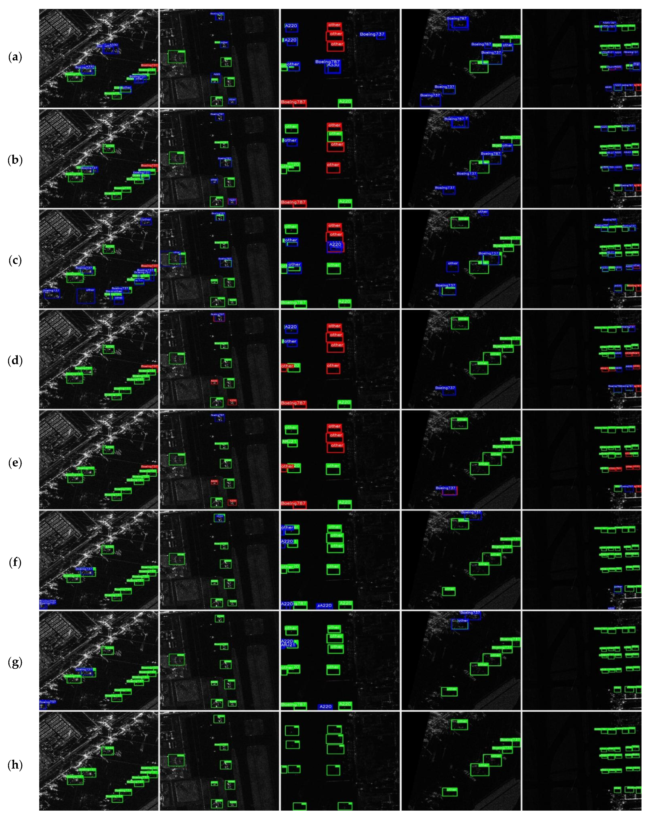
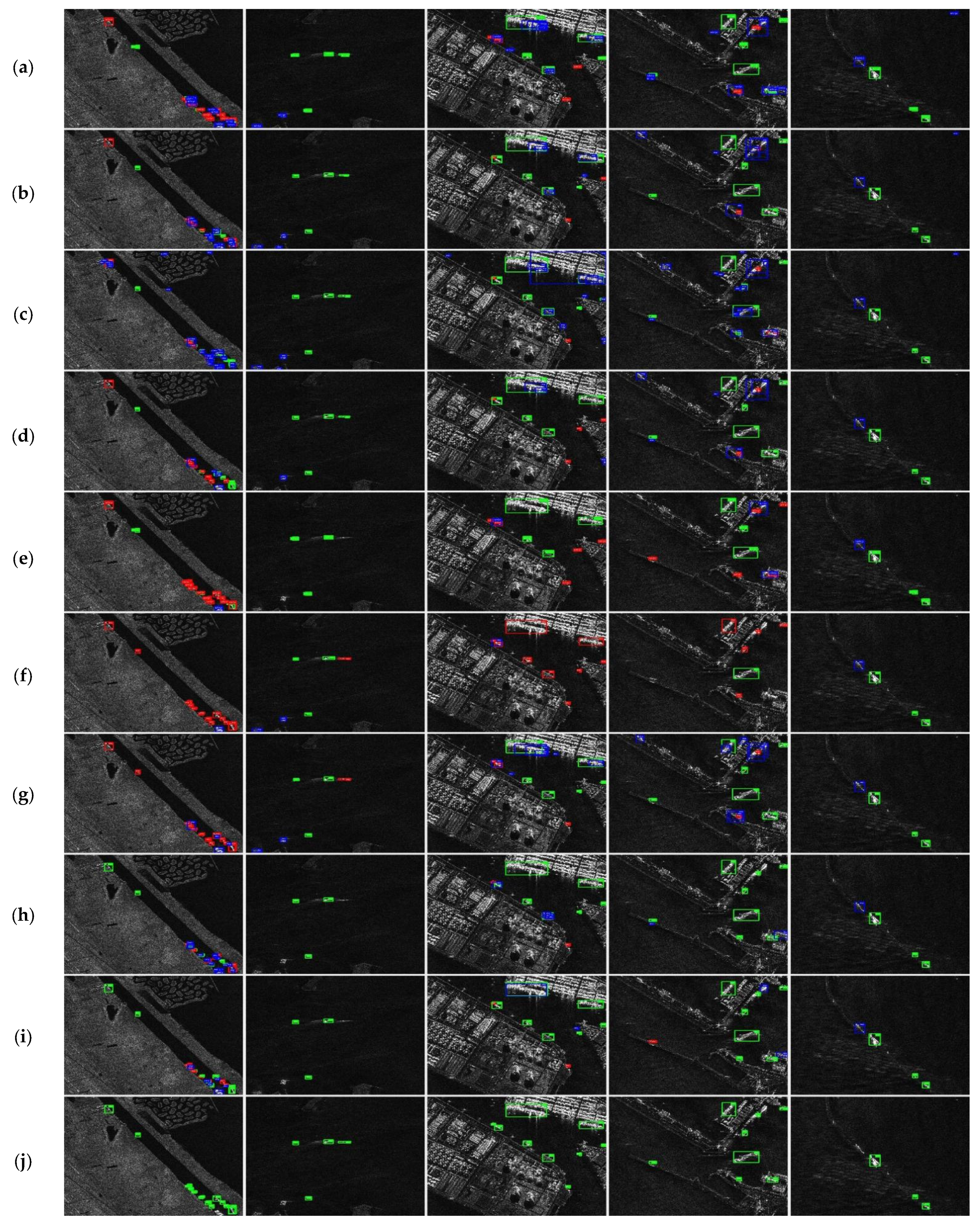
The detection results of all models using ResNet18 as the backbone are visualized for comparison. Five randomly selected images are used for qualitative comparison, with the results of eight detectors presented in Figure 9a–h. In these figures, green, red, and blue bounding boxes denote correctly detected targets, missed detections, and false alarms, respectively. As shown in Figure 9a–e, early detectors such as RetinaNet, GFL, AutoAssign, ATSS, and FOCS suffer from false alarms and missed detections, and duplicate detections frequently occur. This observation indicates insufficient discrimination between targets and complex background clutter. In Figure 9f,g, corresponding to RTMDet and YOLOv10, the number of missed detections is significantly reduced. However, false alarms remain relatively prominent, suggesting that although these methods improve target coverage, their ability to suppress clutter-induced responses is still limited. In Figure 9h, the proposed CGMSN further reduces both false alarms and missed detections while alleviating duplicate detections. Moreover, the predicted bounding boxes exhibit better spatial consistency with the ground-truth targets, indicating improved localization accuracy. These observations are consistent with the metrics achieved by CGMSN in Table 6.

Results on HRSID: The comparison results under the ResNet18 backbone are presented in

Table 7. Comparative experiments on HRSID.

Methods	Backbone	P (%)	R (%)	AP50 (%)	AP75 (%)
RetinaNet [44]	ResNet18	83.9	69.2	78.8	59.8
GFL [45]	ResNet18	91.1	71.6	82.8	62.1
AutoAssign [46]	ResNet18	88.7	73.7	83	62.7
ATSS [47]	ResNet18	87	71.7	81.8	61.8
FCOS [48]	ResNet18	88.6	70.4	81	61.9
DDOD [55]	ResNet18	83.3	59.7	70.3	57.6
FoveaBox [56]	ResNet18	83.8	65.2	75.5	59
RTMDet [49]	ResNet18	93	82.5	90.5	71.3
YOLOv10 [50]	ResNet18	90.9	83.1	90	73.8
CGMSN (Ours)	ResNet18	93.6	87.4	93.3	81.2

. The proposed CGMSN delivers the most favorable performance among all compared detectors. Compared with conventional detectors such as RetinaNet [44], GFL [45], AutoAssign [46], ATSS [47], FCOS [48], Disentangled Dense Object Detector (DDOD) [55], and FoveaBox [56], CGMSN yields consistent improvements across all metrics. It also outperforms recent advanced methods, including RTMDet [49] and YOLOv10 [50], particularly in AP75, indicating better localization quality under stricter evaluation criteria. Although HRSID has a relatively simple background, clear performance differences among detectors still exist. These results suggest the effectiveness and stable performance of the proposed CGMSN in relatively less challenging SAR scenes.

The detection results of RetinaNet, GFL, AutoAssign, ATSS, FCOS, DDOD, FoveaBox, RTMDet, YOLOv10, and the proposed CGMSN, all using ResNet18 as the backbone, are visualized in Figure 10. Three offshore and two nearshore images are selected for comparison. From left to right, the 2nd and 5th columns correspond to offshore images, while the 1st, 3rd, and 4th columns correspond to nearshore images. The color definitions are consistent with Figure 9. As shown in Figure 10a–g, most detectors suffer from false alarms and missed detections. In Figure 10h,i, RTMDet, and YOLOv10 significantly reduce missed detections, especially in offshore scenes, while suppressing false alarms to some extent. In Figure 10j, CGMSN further reduces both missed detections and false alarms across offshore and nearshore scenes. The predicted bounding boxes exhibit better spatial correspondence with the true targets, confirming improved localization consistency. These visual observations are in good agreement with the quantitative results listed in Table 7.

Results on SSDD: The comparison results are presented in

Table 8. Comparative experiments on SSDD.

Methods	DAFDet [57]	RDB-DINO [18]	SwarmPRL [58]	DKMG-Net [59]	TLSA [60]	CGMSN (Ours)
AP50 (%)	98.1	98.3	98.0	98.8	98.7	99.2
AP75 (%)	82.4	90.5	90.7	93.1	93.5	94.0
AP50:95 (%)	68.3	74.7	75.5	77.8	77.8	76.1

. The proposed CGMSN is compared with several recent SAR ship detectors, including DAFDet [57], RDB-DINO [18], SwarmPRL [58], DKMG-Net [59], and Triple-level Sparsity Awareness (TLSA) [60]. CGMSN achieves the best AP50 and AP75 values, reaching 99.2% and 94%, respectively. For AP50:95, CGMSN obtains 76.1%, which is higher than DAFDet, RDB-DINO, and SwarmPRL, but lower than DKMG-Net and TLSA. This suggests that although the proposed method performs well at AP50 and AP75, there is still room for improving localization consistency across a wider range of CIoU thresholds.

5. Discussion

5.1. Relationship Between Target–Background Separability and Fusion Mode

The proposed CFAR target–background separation margin provides an interpretable cue for associating different SAR datasets with different feature-fusion depths. It should be noted that this margin mainly reflects target–background ambiguity in the CFAR anomaly response space, rather than serving as a complete measure of dataset complexity. A smaller margin indicates stronger target–background ambiguity and motivates deeper feature fusion, whereas a larger margin indicates clearer target–background separation and allows a shallower fusion structure.

The mode-comparison results are listed in

Table 9. Detection results on three datasets under three fusion modes.

Dataset	Fusion Mode	P (%)	R (%)	AP50 (%)	AP75 (%)	AP50:95 (%)
SAR-AIRcraft-1.0	D	89.3	94.3	96.7	81.5	72
	M	85.5	92.2	94.4	79.8	68.2
	S	93.73	84.27	93.38	80.38	70.04
HRSID	D	89.8	73.2	84.2	73.8	64.2
	M	93.6	87.4	93.3	81.2	71.9
	S	90.44	87.3	96.13	78.09	69.17
SSDD	D	96.91	89.31	96.67	88.12	73.62
	M	97.15	97.33	99.09	91.55	75.02
	S	97.71	95.68	99.15	93.96	76.01

. On SAR-Aircraft-1.0, D-Mode achieves the best AP50, AP75, and AP50:95, indicating that deeper feature fusion is beneficial for aircraft detection in structured airport environments. In addition, the deeper fusion mode may also help enhance high-level semantic representation and contextual reasoning. On HRSID, M-Mode obtains the best AP75 and AP50:95, suggesting that an intermediate fusion depth provides better localization quality under stricter CIoU thresholds for maritime scenes with moderate target–background ambiguity. On SSDD, S-Mode achieves the best AP50, AP75, and AP50:95, showing that shallower fusion is sufficient when targets are more clearly separated from their surrounding backgrounds. These results suggest that the required feature-fusion depth is related to the CFAR-guided target–background separation margin.

5.2. Complementarity of the Proposed Modules

The ablation results show that the proposed modules contribute from different aspects rather than uniformly improving all metrics in isolation. DCSP mainly enhances contextual representation and feature discrimination. MSN adjusts the feature-fusion depth based on the selected mode, thereby matching the fusion structure to different target–background separability levels. CMH improves classification-regression alignment by modulating prediction confidence according to localization quality. On HRSID, MSN improves precision but may reduce recall, indicating more conservative predictive behavior, whereas CMH can partially mitigate this effect. On SSDD, where the baseline performance is already high, some single-module and dual-module variants show limited gains or slight fluctuations. Nevertheless, the complete model achieves the best overall AP performance across the evaluated datasets. All these results show that the proposed modules provide complementary benefits when used jointly.

5.3. Complexity and Efficiency Considerations

The parameters and FLOPs are mainly determined by the network structure and input resolution, whereas FPS is also affected by batch size, hardware platform, operator implementation, memory access patterns, and feature-map resolution. In the ablation results on the three datasets, the full model reduces the number of parameters and GFLOPs compared with the baseline, but the FPS decreases to some extent. This suggests that lower theoretical complexity does not necessarily result in higher measured inference speed. The decrease in FPS may be related to the memory-access overhead introduced by feature alignment, multi-branch fusion, and other operations in the proposed modules.

6. Conclusions

In this work, CGMSN is proposed for SAR target detection across datasets with different target–background separability levels. First, a CA-CFAR-based target–background separation margin is introduced to characterize dataset-level target–background ambiguity in the CFAR anomaly response space. The proposed margin provides an interpretable cue for selecting an appropriate feature-fusion mode. Then, guided by this separation margin, an improved YOLOv8 model is developed to enable mode-selective target detection. In the backbone, ResNet18 is integrated with a DCSP module to improve contextual feature modeling while maintaining moderate computational cost. In the neck, MSN is designed to provide different feature-fusion modes for SAR datasets with different target–background separability levels. In the head, CMH is proposed to enhance classification-regression alignment by emphasizing reliable predictions and suppressing clutter-affected responses. Experiments on SAR-Aircraft-1.0, HRSID, and SSDD validate the effectiveness of the proposed CGMSN. According to the CFAR-guided target–background separation margin, SAR-Aircraft-1.0, HRSID, and SSDD are assigned to D-Mode, M-Mode, and S-Mode, respectively, and the corresponding results show that matching the feature-fusion mode with dataset-level target–background separability is beneficial for SAR target detection. Moreover, CGMSN achieves superior performance over representative detectors on the three evaluated datasets, indicating its effectiveness across SAR scenes with different characteristics. Although the proposed mode-selection strategy is simple and interpretable, it is still based on discrete dataset-level selection among predefined fusion modes. In future work, we will explore continuously adjustable CFAR-guided fusion mechanisms, such as soft feature weighting and dynamic fusion-depth control. More comprehensive hardware-aware evaluations, including latency analysis and embedded-GPU deployment, will also be conducted to further assess the practical applicability of the proposed network.

References

1. Tian, Y.; Gao, F.; Huang, R.; Wu, Y. HGXES: Lightweight network for ship detection in specific marine environments. Remote Sens. 2026, 18, 1276. [Google Scholar] [CrossRef]
2. Ai, J.; Mao, Y.; Luo, Q.; Xing, M.; Jiang, K.; Jia, L.; Yang, X. Robust CFAR ship detector based on bilateral-trimmed-statistics of complex ocean scenes in SAR imagery: A closed-form solution. IEEE Trans. Aerosp. Electron. Syst. 2021, 57, 1872–1890. [Google Scholar] [CrossRef]
3. Li, Y.; Zhang, S.; Wang, W.-Q. A lightweight Faster R-CNN for ship detection in SAR images. IEEE Geosci. Remote Sens. Lett. 2022, 19, 4006105. [Google Scholar] [CrossRef]
4. Chai, B.; Nie, X.; Zhou, Q.; Zhou, X. Enhanced cascade R-CNN for multiscale object detection in dense scenes from SAR images. IEEE Sens. J. 2024, 24, 20143–20153. [Google Scholar] [CrossRef]
5. Zhou, P.; Niu, B.; Huang, L.; Wang, Q.; Zhao, Y.; Zhou, G.; Hu, Y. SARDet-MIM: Enhancing SAR target detection via a structural and scattering masked autoencoder. Remote Sens. 2026, 18, 580. [Google Scholar] [CrossRef]
6. Tan, X.; Leng, X.; Luo, R.; Sun, Z.; Ji, K.; Kuang, G. YOLO-RC: SAR ship detection guided by characteristics of range-compressed domain. IEEE J. Sel. Top. Appl. Earth Obs. Remote Sens. 2024, 17, 18834–18851. [Google Scholar] [CrossRef]
7. Liu, H.; Dong, H.; Shi, H.; Li, F. CCAI-YOLO: A high-precision synthetic aperture radar ship detection model based on YOLOv8n algorithm. Remote Sens. 2026, 18, 145. [Google Scholar] [CrossRef]
8. Wang, Z.; Du, L.; Mao, J.; Liu, B.; Yang, D. SAR target detection based on SSD with data augmentation and transfer learning. IEEE Geosci. Remote Sens. Lett. 2019, 16, 150–154. [Google Scholar] [CrossRef]
9. Xu, X.; Bai, Y.; Liu, G.; Zhang, P. Lite-YOLOv5: A lightweight deep learning detector for on-board ship detection in large-scene Sentinel-1 SAR images. Remote Sens. 2022, 14, 1018. [Google Scholar] [CrossRef]
10. Lin, H.; Liu, J.; Li, X.; Wei, L.; Liu, Y.; Han, B.; Wu, Z. DCEA: DETR with concentrated deformable attention for end-to-end ship detection in SAR images. IEEE J. Sel. Top. Appl. Earth Obs. Remote Sens. 2024, 17, 17292–17307. [Google Scholar] [CrossRef]
11. Li, C.; Hei, Y.; Xi, L.; Li, W.; Xiao, Z. GL-DETR: Global-to-local transformers for small ship detection in SAR images. IEEE Geosci. Remote Sens. Lett. 2024, 21, 4016805. [Google Scholar] [CrossRef]
12. Ai, J.; Tian, R.; Luo, Q.; Jin, J.; Tang, B. Multi-scale rotation-invariant Haar-like feature integrated CNN-based ship detection algorithm of multiple-target environment in SAR imagery. IEEE Trans. Geosci. Remote Sens. 2019, 57, 10070–10087. [Google Scholar] [CrossRef]
13. Ma, X.; Hou, S.; Wang, Y.; Wang, J.; Wang, H. Multiscale and dense ship detection in SAR images based on key-point estimation and attention mechanism. IEEE Trans. Geosci. Remote Sens. 2022, 60, 5221111. [Google Scholar] [CrossRef]
14. Yang, S.; An, W.; Li, S.; Wei, G.; Zou, B. An improved FCOS method for ship detection in SAR images. IEEE J. Sel. Top. Appl. Earth Obs. Remote Sens. 2022, 15, 8910–8927. [Google Scholar] [CrossRef]
15. Yue, T.; Zhang, Y.; Wang, J.; Xu, Y.; Liu, P. A weak supervision learning paradigm for oriented ship detection in SAR image. IEEE Trans. Geosci. Remote Sens. 2024, 62, 5207812. [Google Scholar] [CrossRef]
16. Li, Y.; Liu, J.; Li, X.; Zhang, X.; Wu, Z.; Han, B. A lightweight network for ship detection in SAR images based on edge feature aware and fusion. IEEE J. Sel. Top. Appl. Earth Obs. Remote Sens. 2025, 18, 3782–3796. [Google Scholar] [CrossRef]
17. Feng, Y.; Zhang, Y.; Zhang, X.; Wang, Y.; Mei, S. Large convolution kernel network with edge self-attention for oriented SAR ship detection. IEEE J. Sel. Top. Appl. Earth Obs. Remote Sens. 2025, 18, 2867–2879. [Google Scholar] [CrossRef]
18. Qin, C.; Zhang, L.; Wang, X.; Li, G.; He, Y.; Liu, Y. RDB-DINO: An improved end-to-end transformer with refined de-noising and boxes for small-scale ship detection in SAR images. IEEE Trans. Geosci. Remote Sens. 2025, 63, 5200517. [Google Scholar] [CrossRef]
19. Zhou, S.; Zhang, M.; Wu, L.; Yu, D.; Li, J.; Fan, F. Lightweight SAR ship detection network based on transformer and feature enhancement. IEEE J. Sel. Top. Appl. Earth Obs. Remote Sens. 2024, 17, 4845–4858. [Google Scholar] [CrossRef]
20. Zeng, J.; Tang, X.; Li, S. DAFE-Net: Direction-aware feature enhancement network for SAR ship detection. Remote Sens. 2026, 18, 1380. [Google Scholar] [CrossRef]
21. Wang, Z.; Kang, Y.; Zeng, X.; Wang, Y.; Zhang, T.; Sun, X. SAR-Aircraft-1.0: High-resolution SAR aircraft detection and recognition dataset. J. Radars 2023, 12, 906–922. [Google Scholar] [CrossRef]
22. Wei, S.; Zeng, X.; Qu, Q.; Wang, M.; Su, H.; Shi, J. HRSID: A high-resolution SAR images dataset for ship detection and instance segmentation. IEEE Access 2020, 8, 120234–120254. [Google Scholar] [CrossRef]
23. Zhang, T.; Zhang, X.; Li, J.; Xu, X.; Wang, B.; Zhan, X.; Xu, Y.; Ke, X.; Zeng, T.; Su, H.; et al. SAR Ship Detection Dataset (SSDD): Official Release and Comprehensive Data Analysis. Remote Sens. 2021, 13, 3690. [Google Scholar] [CrossRef]
24. Luo, C.; Zhang, Y.; Guo, J.; Zhou, G.; You, H.; Li, P.; Ning, X. DEMC: A diffusion-enhanced mutual consistency framework for cross-domain object detection in optical and SAR imagery. Remote Sens. 2026, 18, 1358. [Google Scholar] [CrossRef]
25. Zhao, S.; Luo, Y.; Zhang, T.; Guo, W.; Zhang, Z. A feature decomposition-based method for automatic ship detection crossing different satellite SAR images. IEEE Trans. Geosci. Remote Sens. 2022, 60, 5234015. [Google Scholar] [CrossRef]
26. Pan, B.; Xu, Z.; Shi, T.; Li, T.; Shi, Z. An imbalanced discriminant alignment approach for domain adaptive SAR ship detection. IEEE Trans. Geosci. Remote Sens. 2023, 61, 5108111. [Google Scholar] [CrossRef]
27. Zhang, X.; Zhang, S.; Sun, Z.; Liu, C.; Sun, Y.; Ji, K.; Kuang, G. Cross-sensor SAR image target detection based on dynamic feature discrimination and center-aware calibration. IEEE Trans. Geosci. Remote Sens. 2025, 63, 5209417. [Google Scholar] [CrossRef]
28. Du, W.; Cheng, J.; Zhang, C.; Zhao, P.; Wan, H.; Zhou, Z. SARNas: A hardware-aware SAR target detection algorithm via multiobjective neural architecture search. IEEE Trans. Geosci. Remote Sens. 2023, 61, 5212923. [Google Scholar] [CrossRef]
29. Kuang, C.; Wang, C.; Wen, B.; Hou, Y.; Lai, Y. An improved CA-CFAR method for ship target detection in strong clutter using UHF radar. IEEE Signal Process. Lett. 2020, 27, 1445–1449. [Google Scholar] [CrossRef]
30. El-Darymli, K.; McGuire, P.; Power, D.; Moloney, C. Target detection in synthetic aperture radar imagery: A state-of-the-art survey. J. Appl. Remote Sens. 2013, 7, 071598. [Google Scholar] [CrossRef]
31. Li, T.; Peng, D.; Chen, Z.; Guo, B. Superpixel-level CFAR detector based on truncated gamma distribution for SAR images. IEEE Geosci. Remote Sens. Lett. 2021, 18, 1421–1425. [Google Scholar] [CrossRef]
32. Yang, H.; Zhang, T.; He, Y.; Dan, Y.; Yin, J.; Ma, B.; Yang, J. GPU-oriented designs of constant false alarm rate detectors for fast target detection in radar images. IEEE Trans. Geosci. Remote Sens. 2022, 60, 5231214. [Google Scholar] [CrossRef]
33. Wang, C.; Guo, B.; Song, J.; He, F.; Li, C. A novel CFAR-based ship detection method using range-compressed data for spaceborne SAR system. IEEE Trans. Geosci. Remote Sens. 2024, 62, 5215515. [Google Scholar] [CrossRef]
34. Zhao, Y.; Zhao, L.; Li, C.; Kuang, G. Pyramid attention dilated network for aircraft detection in SAR images. IEEE Geosci. Remote Sens. Lett. 2021, 18, 662–666. [Google Scholar] [CrossRef]
35. Guo, Q.; Wang, H.; Xu, F. Scattering enhanced attention pyramid network for aircraft detection in SAR images. IEEE Trans. Geosci. Remote Sens. 2021, 59, 7570–7587. [Google Scholar] [CrossRef]
36. Chen, Y.; Cong, Y.; Zhang, L. Deformable scattering feature correlation network for aircraft detection in SAR images. IEEE Geosci. Remote Sens. Lett. 2023, 20, 4007205. [Google Scholar] [CrossRef]
37. Kang, Y.; Wang, Z.; Fu, J.; Sun, X.; Fu, K. SFR-Net: Scattering feature relation network for aircraft detection in complex SAR images. IEEE Trans. Geosci. Remote Sens. 2022, 60, 5218317. [Google Scholar] [CrossRef]
38. Chen, L.; Luo, R.; Xing, J.; Li, Z.; Yuan, Z.; Cai, X. Geospatial transformer is what you need for aircraft detection in SAR imagery. IEEE Trans. Geosci. Remote Sens. 2022, 60, 5225715. [Google Scholar] [CrossRef]
39. Zhou, J.; Xiao, C.; Peng, B.; Liu, Z.; Liu, L.; Liu, Y. DiffDet4SAR: Diffusion-based aircraft target detection network for SAR images. IEEE Geosci. Remote Sens. Lett. 2024, 21, 4007905. [Google Scholar] [CrossRef]
40. Luo, R.; He, Q.; Zhao, L.; Zhang, S.; Kuang, G.; Ji, K. Geospatial contextual prior-enabled knowledge reasoning framework for fine-grained aircraft detection in panoramic SAR imagery. IEEE Trans. Geosci. Remote Sens. 2024, 62, 5226213. [Google Scholar] [CrossRef]
41. Peng, Y.; Chen, D.Z.; Sonka, M. U-Net V2: Rethinking the skip connections of U-Net for medical image segmentation. In Proceedings of the IEEE 22nd International Symposium on Biomedical Imaging, Houston, TX, USA, 14–17 April 2025. [Google Scholar]
42. Cui, Z.; Wang, X.; Liu, N.; Cao, Z.; Yang, J. Ship detection in large-scale SAR images via spatial shuffle-group enhance attention. IEEE Trans. Geosci. Remote Sens. 2021, 59, 379–391. [Google Scholar] [CrossRef]
43. Chang, H.; Fu, X.; Lang, P.; Guo, K.; Dong, J.; Chang, S. GLDet: Real-time SAR ship detector based on global semantic information enhancement and local gradient information mining. IEEE Trans. Geosci. Remote Sens. 2025, 63, 5209020. [Google Scholar] [CrossRef]
44. Lin, T.-Y.; Goyal, P.; Girshick, R.; He, K.; Dollár, P. Focal loss for dense object detection. IEEE Trans. Pattern Anal. Mach. Intell. 2020, 42, 318–327. [Google Scholar] [CrossRef] [PubMed]
45. Li, X.; Wang, W.; Wu, L.; Chen, S.; Hu, X.; Li, J.; Tang, J.; Yang, J. Generalized focal loss: Learning qualified and distributed bounding boxes for dense object detection. In Proceedings of the Advances in Neural Information Processing Systems, Virtual, 6–12 December 2020; pp. 21002–21012. [Google Scholar]
46. Zhu, B.; Wang, J.; Jiang, Z.; Zong, F.; Liu, S.; Li, Z.; Sun, J. AutoAssign: Differentiable label assignment for dense object detection. arXiv 2020, arXiv:2007.03496. [Google Scholar] [CrossRef]
47. Zhang, S.; Chi, C.; Yao, Y.; Lei, Z.; Li, S.Z. Bridging the gap between anchor-based and anchor-free detection via adaptive training sample selection. In Proceedings of the IEEE/CVF Conference on Computer Vision and Pattern Recognition, Seattle, WA, USA, 13–19 June 2020; pp. 9756–9765. [Google Scholar]
48. Tian, Z.; Shen, C.; Chen, H.; He, T. FCOS: Fully convolutional one-stage object detection. In Proceedings of the IEEE/CVF International Conference on Computer Vision, Seoul, Republic of Korea, 27 October–2 November 2019; pp. 9626–9635. [Google Scholar]
49. Lyu, C.; Zhang, W.; Huang, H.; Zhou, Y.; Wang, Y.; Liu, Y.; Zhang, S.; Chen, K. RTMDet: An empirical study of designing real-time object detectors. arXiv 2022, arXiv:2212.07784. [Google Scholar] [CrossRef]
50. Ao, W.; Chen, H.; Liu, L.; Chen, K.; Lin, Z.; Han, J.; Ding, G. YOLOv10: Real-time end-to-end object detection. arXiv 2024, arXiv:2405.14458. [Google Scholar] [CrossRef]
51. Girshick, R. Fast R-CNN. In Proceedings of the IEEE International Conference on Computer Vision, Santiago, Chile, 7–13 December 2015; pp. 1440–1448. [Google Scholar]
52. Cai, Z.; Vasconcelos, N. Cascade R-CNN: Delving into high quality object detection. In Proceedings of the IEEE/CVF Conference on Computer Vision and Pattern Recognition, Salt Lake City, UT, USA, 18–23 June 2018; pp. 6154–6162. [Google Scholar]
53. Yang, Z.; Liu, S.; Hu, H.; Wang, L.; Lin, S. RepPoints: Point set representation for object detection. In Proceedings of the IEEE/CVF International Conference on Computer Vision, Seoul, Republic of Korea, 27 October–2 November 2019; pp. 9656–9665. [Google Scholar]
54. Fu, K.; Fu, J.; Wang, Z.; Sun, X. Scattering-keypoint-guided network for oriented ship detection in high-resolution and large-scale SAR images. IEEE J. Sel. Top. Appl. Earth Obs. Remote Sens. 2021, 14, 11162–11178. [Google Scholar] [CrossRef]
55. Chen, Z.; Yang, C.; Li, Q.; Zhao, F.; Zha, Z.-J.; Wu, F. Disentangle your dense object detector. In Proceedings of the 29th ACM International Conference on Multimedia, Chengdu, China, 20–24 October 2021; pp. 4939–4948. [Google Scholar]
56. Kong, T.; Sun, F.; Liu, H.; Jiang, Y.; Li, L.; Shi, J. FoveaBox: Beyond anchor-based object detection. IEEE Trans. Image Process. 2020, 29, 7389–7398. [Google Scholar] [CrossRef]
57. Yang, Y.; Du, Y.; Zhang, L.; Li, G.; Chen, Y.; Cheng, G.; Song, S. DAFDet: A Unified Dynamic SAR Target Detection Architecture with Asymptotic Fusion Enhancement and Feature Encoding Decoupling. IEEE Trans. Geosci. Remote Sens. 2025, 63, 5201922. [Google Scholar] [CrossRef]
58. Zhang, T.; Gao, G.; Ke, X.; Zhang, X. Swarm Learning: Perception–Retrieval–Localization for Ship Detection from Synthetic Aperture Radar Remote Sensing Imagery. IEEE J. Sel. Top. Appl. Earth Obs. Remote Sens. 2026, 19, 12384–12395. [Google Scholar] [CrossRef]
59. Zhang, T.; Zhang, X.; Gao, G. Density Knowledge Mining for Quantity-Aware Marine Vessel Surveillance Using Satellite SAR Data. IEEE Trans. Ind. Inform. 2026, 22, 5173–5184. [Google Scholar] [CrossRef]
60. Zhang, T.; Zhang, X. Triple-Level Sparsity Awareness for Marine Ship Surveillance Using Satellite Synthetic Aperture Radar. IEEE Trans. Autom. Sci. Eng. 2026, 23, 5155–5166. [Google Scholar] [CrossRef]
Figure 1. Representative SAR scenes from three different datasets. (a) SAR-Aircraft-1.0 dataset with structured airport backgrounds. (b) High-Resolution SAR Images Dataset (HRSID) with coastal maritime backgrounds. (c) SAR Ship Detection Dataset (SSDD) with relatively homogeneous sea-dominated backgrounds. The first row shows the original images with ground-truth bounding boxes, while the second row shows the corresponding constant false alarm rate (CFAR) anomaly response maps computed using Equation (5) in Section 3.
Remotesensing 18 02040 g001
Figure 2. The overall framework of the CFAR-guided mode-selective network (CGMSN). (a) Calculation of the cell-averaging CFAR (CA-CFAR)-guided dataset-level target–background separation margin. (b) Backbone with ResNet18 and the dilated convolutional spatial pyramid (DCSP) module. (c) Mode-selection neck (MSN). (d) Complete intersection over the union modulated head (CMH). SDI-GSC denotes semantic and detail infusion and grouped shuffle convolution.
Remotesensing 18 02040 g002
Figure 3. Structures of the dilated convolutional spatial pyramid (DCSP) module and the spatial pyramid pooling-fast (SPPF) module. (a) DCSP. (b) SPPF.
Remotesensing 18 02040 g003
Figure 4. Three feature-fusion modes in the mode-selective neck (MSN). (a) Deep feature-fusion mode (D-Mode) and medium feature-fusion mode (M-Mode). (b) Shallow feature-fusion mode (S-Mode).
Remotesensing 18 02040 g004
Figure 5. Structure of the semantic and detail infusion and grouped shuffle convolution (SDI-GSC) module. (a) SDI-GSC, which performs scale alignment and feature fusion among different branches. (b) Grouped shuffle convolution (GSC), which enhances channel interaction with moderate computational cost.
Remotesensing 18 02040 g005
Figure 6. (a) Baseline. (b) Baseline + DCSP. (c) Baseline + DCSP + MSN. (d) Baseline + DCSP + MSN + CMH. (e) Ground truth.
Remotesensing 18 02040 g006
Figure 7. (a) Baseline. (b) Baseline + DCSP. (c) Baseline + DCSP + MSN. (d) Baseline + DCSP + MSN + CMH. (e) Ground truth.
Remotesensing 18 02040 g007
Figure 8. (a) Baseline. (b) Baseline + DCSP. (c) Baseline + DCSP + MSN. (d) Baseline + DCSP + MSN + CMH. (e) Ground truth.
Remotesensing 18 02040 g008
Figure 9. Visual comparison of detection results on SAR-Aircraft-1.0. (a) RetinaNet. (b) Generalized Focal Loss (GFL). (c) AutoAssign. (d) Adaptive Training Sample Selection (ATSS). (e) Fully Convolutional One-Stage Object Detection (FCOS). (f) RTMDet. (g) You Only Look Once version 10 (YOLOv10). (h) CGMSN (Ours). Green, red, and blue bounding boxes denote correctly detected targets, missed detections, and false alarms, respectively.
Remotesensing 18 02040 g009
Figure 10. Visual comparison of detection results on HRSID. (a) RetinaNet. (b) GFL. (c) AutoAssign. (d) ATSS. (e) FCOS. (f) Disentangled Dense Object Detector (DDOD). (g) FoveaBox. (h) RTMDet. (i) YOLOv10. (j) CGMSN (Ours). From left to right, the second and fifth columns show offshore SAR scenes, while the first, third, and fourth columns show nearshore SAR scenes. Green, red, and blue bounding boxes indicate correctly detected targets, missed detections, and false alarms, respectively.
Remotesensing 18 02040 g010