


Highlights
What are the main findings?
- Across 20 vision architectures, geospatial manipulation families exhibited distinct and consistent failure modes: subtle pixel-level perturbations were most often confused with authentic imagery, localized generative inpainting generalized poorly under source shift, and adversarial patch detection transferred more reliably across unseen geometries than pixel-level detection transferred across perturbation budgets.
- Strong balanced in-domain benchmark performance did not reliably translate to operational screening utility. Under external-domain transfer and low-prevalence conditions, several models produced high false-alarm burdens, while limited-label target-domain adaptation substantially improved detection and screening performance.
What is the implication of the main finding?
- Geospatial manipulation detectors should be evaluated beyond balanced in-domain accuracy, using source-shift testing, attack-variant stress tests, external-domain transfer, adaptation behavior, augmentation sensitivity, and low-prevalence false-alarm metrics that better reflect operational deployment conditions.
- Model selection should align with deployment objectives: specialized binary detectors are preferable when the manipulation family is known in advance, whereas unified multi-attack models are better suited for analyst workflows that require both manipulation screening and attribution of the likely attack family.
Abstract
Manipulated satellite imagery threatens analytic workflows, policy decisions, and trust in geospatial intelligence. Operational systems increasingly benefit from capabilities for both manipulation detection and manipulation-family attribution to support verification, triage, and downstream analysis. We present a unified benchmark for characterizing three representative manipulation families in geospatial imagery—generative manipulations, pixel-level perturbations, and adversarial patches—using a controlled, class-balanced design and 20 modern vision architectures spanning conventional, Earth-observation-pretrained, and vision-language models. Across architectures, the dominant failure boundary is between authentic imagery and subtle pixel-level perturbations, whereas generative manipulations and adversarial patches are generally more separable under matched in-domain conditions. Additional analyses reveal important generalization limitations under unseen manipulation variants and external-domain transfer, demonstrating that strong benchmark performance does not necessarily translate to reliable operational screening. The framework also enables systematic comparison of unified multi-attack and specialized detection strategies, providing insight into their relative strengths and limitations. Rather than proposing a new defense, this work provides a reproducible methodology for characterizing manipulation artifacts, model failure modes, and deployment-relevant screening behavior in geospatial imagery, with applications to analyst triage, verification workflows, and trustworthy use of satellite data.
1. Introduction
We conduct a detailed study on how modern vision models, including supervised, EO-pretrained, and vision-language architectures, characterize and distinguish multiple adversarial manipulation types in geospatial imagery. Satellite and geospatial imagery underpin critical applications in environmental monitoring, disaster response, sanctions enforcement, treaty verification, and national security. As generative AI and adversarial manipulation techniques continue to advance, these data streams have become increasingly vulnerable to falsification. Recent reporting has documented “deepfake geography” and fabricated satellite scenes that can distort situational awareness and erode trust in geospatial evidence [1,2]. Such threats impose not only analytic risk but operational cost: analysts must determine not simply whether an image is manipulated, but what kind of manipulation has occurred to support triage, attribution, and verification workflows.
At the same time, the broader adversarial ML and deepfake detection literature highlights fundamental challenges. Robust detection is closely tied to robust classification, and detectors frequently fail when confronted with unseen or adaptive attacks [3,4]. However, these findings largely arise from natural-image settings with white-box threat models. In contrast, geospatial manipulation is typically conducted under black-box or weakly adaptive conditions: adversaries lack access to detector internals, and manipulations must remain consistent with physical and spectral constraints such as lighting, shadow geometry, terrain structure, and multispectral coherence. Moreover, EO products are shaped by sensing and processing pipelines (e.g., resampling/orthorectification and compression) and wide resolution variation, so subtle perturbations can resemble acquisition artifacts rather than overt edits. Finally, overhead targets often have small footprints, making object-centric manipulations and object-centric screening particularly relevant in geospatial workflows. This structured domain motivates a different line of inquiry—not the design of new defenses, but the characterization of how diverse attack types present to modern models and where confusion arises.
Prior work in remote sensing has shown that pixel-level perturbations can reliably alter land-cover and scene-classification predictions [5], while localized adversarial patches can induce false positives or negatives in aerial object detectors [6]. Generative manipulations can introduce either fully synthetic scenes or localized synthetic edits that remain visually plausible.
Yet these attack families are typically studied in isolation, making it difficult to compare their impact on model behavior or assess whether cues learned from one manipulation transfer to another. Moreover, despite the strategic importance of geospatial imagery, surprisingly little work has systematically analyzed how diverse adversarial manipulations present to modern vision models in the geospatial domain.
In this work, we conduct a unified analysis of three representative adversarial manipulation families in satellite imagery:
- Global and local generative manipulations [7];
- Pixel-level adversarial perturbations [8,9,10]; and
- Localized adversarial patches [11,12,13].
Using a controlled, class-balanced design and a diverse set of 20 vision architectures spanning supervised, EO-pretrained, and vision-language settings, as illustrated in Figure 1, we treat attack-type identification as a four-way manipulation characterization task. Rather than proposing a new defense architecture, our goal is to determine where modern models succeed, where they confuse manipulation families, and how these behaviors change under source shift, attack-parameter shift, external-domain transfer, and deployment-relevant training choices. We examine four research questions (RQs):
Figure 1.
Overview of the study design. Real and generative geospatial image sources are used to construct controlled REAL, PIXEL, PATCH, and FAKE classes. The benchmark trains unified four-way models and specialized binary detectors, then evaluates in-domain separability, FAKE source-shift generalization, PIXEL/PATCH attack-variant generalization, external-domain transfer and adaptation, augmentation sensitivity, and low-prevalence triage behavior.
- RQ1: In-domain separability. Which manipulation families are most separable or most easily confused in a controlled four-way REAL/PIXEL/PATCH/FAKE benchmark across modern vision architectures?
- RQ2: Attack-variant and source-shift generalization. Do learned manipulation cues generalize to unseen FAKE generation mechanisms, reduced or increased PIXEL perturbation budgets, and unseen PATCH geometry?
- RQ3: Unified versus specialized detection. When are unified multi-attack models preferable to specialized binary REAL/attack detectors, and how does this comparison change under in-domain testing, external-domain transfer, and limited-label target-domain adaptation?
- RQ4: Deployment sensitivity. How do practical design choices such as augmentation severity and low-prevalence triage assumptions affect manipulation screening performance?
Key findings. Across the 20-model in-domain benchmark, the dominant confusion boundary is REAL↔PIXEL: subtle pixel-level perturbations are most often confused with clean imagery, while PATCH and FAKE are generally more separable under matched in-domain conditions. However, high in-domain FAKE performance does not imply generator-robust FAKE detection. Leave-one-method-out (LOMO) experiments show that FAKE recognition is strongly source-dependent, with localized inpainting especially difficult when excluded from training. Attack-variant stress tests further show that PATCH detection transfers well to an unseen square-patch geometry, whereas PIXEL detection is highly sensitive to the saliency-seed budget: the lower-budget PIXEL setting produces substantially more PIXEL→REAL missed detections. Specialized binary detectors usually outperform unified multi-attack models on pairwise REAL/attack tasks, both in-domain and under zero-adaptation external-domain transfer, although limited-label target-domain adaptation narrows this gap. Finally, deployment-facing evaluation shows that balanced benchmark performance is not sufficient for operational screening: unadapted external-domain models produce poor low-prevalence triage behavior, while target-domain adaptation substantially reduces the false-alarm burden for several architectures.
By answering these questions, we provide insight into cross-attack separability, source-shift generalization, external-domain transfer, and deployment tradeoffs within a structured, physically grounded domain. Our findings offer practical guidance for operational screening pipelines and establish a reproducible benchmark with shared metrics and diagnostics for characterizing adversarial manipulations in geospatial imagery.
Contribution and scope. The individual attacks and architectures evaluated here are not themselves the primary novelty. Instead, the contribution is the controlled organization of multiple manipulation families into a unified geospatial characterization protocol. This benchmark is intentionally controlled rather than a complete operational threat model. The PIXEL and PATCH manipulations are not intended to exhaustively represent all realistic adversarial threats in remote sensing; instead, they provide reproducible manipulation families that isolate different visual signatures: sparse low-amplitude perturbations, localized structured patches, and global or local generative edits. This design reveals stable failure boundaries, source-shift weaknesses, unified-versus-specialized tradeoffs, and training sensitivities that are difficult to observe in isolated single-attack or binary robustness studies. The benchmark should therefore be interpreted as a diagnostic artifact characterization benchmark for geospatial manipulation screening, where analysts may need not only a manipulated/not-manipulated decision but also evidence about the likely manipulation family.
Contributions. (1) We define a controlled four-way manipulation identification task (REAL/PIXEL/PATCH/FAKE) with class balance, scene-disjoint splits, and matched-base imagery for REAL/PIXEL/PATCH to isolate manipulation artifacts from scene content. (2) We benchmark 20 modern vision architectures under a shared protocol, spanning conventional CNNs, general-purpose Transformers, EO-pretrained models, and vision-language remote-sensing models, and report cross-family confusion structure and class-wise performance. (3) We evaluate attack-variant and source-shift generalization through FAKE leave-one-method-out testing, PIXEL cross-budget testing, and PATCH unseen-style testing. (4) We compare specialized binary REAL/attack detectors against unified multi-attack models under in-domain testing, zero-adaptation external-domain transfer, and limited-label target-domain adaptation. (5) We analyze deployment-relevant training and screening choices, including augmentation severity, prevalence-adjusted precision, and false-alarm burden under low-prevalence triage.
2. Related Work
Manipulated satellite imagery (deepfakes). Early work on “deep fake geography” showed that generative models can synthesize city-scale satellite scenes that visually and statistically resemble reality, raising urgent concerns for GIS, disaster response, and security, and arguing for remote-sensing (RS)-specific forensics rather than repurposed natural-image detectors [7]. Subsequent efforts moved toward detection benchmarks and larger RS-specific forged/real corpora (e.g., diffusion-based overhead datasets with localization labels), reflecting a shift from proofs of concept to broad evaluations of detector robustness in overhead settings [14].
Pixel-level perturbations in RS. Czaja et al. were among the first in remote sensing to show that very small, often invisible pixel changes can fool classifiers on single images and across time, and they highlighted RS-specific issues such as changing viewpoints and temporal drift [15]. Follow-up RS studies introduced universal (image-agnostic) perturbations and black-box attacks tailored to RS (e.g., UAE-RS), demonstrating strong transfer across architectures and tasks (scene classification, segmentation) [5]. These observations align with foundational vision results on universal perturbations and cross-model transferability [16].
Adversarial patches in overhead imagery. Unlike small-norm perturbations, patches are localized and visible yet highly salient and transformation-robust. Physical-world patch attacks have been optimized, fabricated, and deployed on or near targets to substantially reduce aerial object-detector efficacy under altitude, pose, and illumination changes [6]. Beyond detection, recent work evaluates patch threats and proposes architecture-level defenses for aerial semantic segmentation, underscoring the need for patch-aware robustness in RS models [17,18].
Forensics and RS-specific detection surveys. A growing RS forensics literature surveys manipulation strategies (inpainting, splicing, synthesis) and corresponding detection cues, emphasizing that detectors often overfit to generator-specific artifacts and may not generalize to unseen methods which directly motivates our multi-attack evaluations and error analysis [19,20]. Larger, RS-native fake/real datasets now enable cross-generator testing protocols that mirror these concerns [14].
Unlike surveys that catalog manipulation types and forensic cues, this study provides an empirical characterization of how modern vision models distinguish multiple manipulation families under a shared remote-sensing protocol. Prior RS deepfake detection work has typically focused on REAL versus FAKE discrimination, often for a single generator or synthetic-image source. In contrast, we evaluate FAKE alongside PIXEL and PATCH manipulations and explicitly test whether FAKE cues transfer across generation mechanisms, including both global synthetic imagery and localized inpainting.
Our study also differs from prior pixel-level adversarial perturbation work in remote sensing. Existing perturbation studies primarily ask whether small pixel changes can fool classifiers, segmentation models, or other downstream RS systems. Here, we instead ask whether trained detectors can recognize such perturbations as a manipulation family and where they confuse PIXEL examples with authentic imagery. This distinction is important because a manipulation may be successful as an attack while remaining difficult to detect or characterize in a forensic screening pipeline.
Similarly, prior adversarial patch work in overhead imagery has largely emphasized attack success against aerial object detectors or segmentation models. Our goal is different: we evaluate whether localized patch artifacts are recognizable as a manipulation class and whether the learned cues transfer when patch geometry changes. This allows PATCH behavior to be compared directly against PIXEL and FAKE behavior under the same model families, metrics, and train/test controls.
Finally, while general fake-image detection studies have examined cross-generator generalization in natural-image settings, our experiments test this question specifically in geospatial imagery, where scene structure, resolution, acquisition artifacts, and local object footprints differ from ordinary photographs. This framing reveals failure modes that are difficult to observe in isolated binary evaluations, including REAL–PIXEL ambiguity, generator/source dependence within FAKE, and the different transfer behavior of localized patches versus sparse pixel-level perturbations.
Cross-attack generalization and transfer. Evidence from RS and general synthetic-image detection suggests that detectors can pick up manipulation-agnostic cues (e.g., frequency/texture inconsistencies), yet cross-manipulation generalization remains fragile without explicit training signals. Work on universal perturbations and RS black-box attacks shows transfer across models and tasks [5,16], while recent “universal fake image” detectors highlight strategies for cross-generator generalization that inform our question of whether multi-attack training helps a specific attack class [21].
Data augmentation and robustness. Augmentation is a major lever for both clean-accuracy generalization and robustness. Mixup and CutMix (mixed-sample augmentations) are linked to smoother decision boundaries and improved robustness [22,23] while AugMix targets corruption robustness [24]. Robustness studies show that augmentation choice and scheduling matter since certain compositions, especially when paired with weight averaging, can materially improve adversarial robustness [25]. RS surveys further document which geometric/photometric transforms tend to help aerial tasks, guiding our design space in the data augmentations section of this paper [26].
Operational screening and triage. Most robustness studies report balanced test accuracy or attack-specific recall under curated evaluation sets. Operational geospatial screening, however, often involves low-prevalence conditions in which manipulated imagery is rare relative to authentic imagery. In such settings, high balanced accuracy may still correspond to unacceptable false alarm rates, and precision–recall behavior becomes more informative than accuracy alone. This motivates our use of deployment-facing metrics such as manipulated-class precision, recall, AUPRC, and false alarms under simulated class-imbalance settings.
3. Materialsand Methods
Adversarial manipulation in satellite imagery spans global generative edits, sparse pixel-level perturbations, and localized patches. Because these families differ in both appearance and how modern detectors perceive them, we evaluate them in a unified, controlled framework. We study three representative cases—generative FAKE imagery, gradient-guided pixel perturbations, and learnable adversarial patches. We use a frozen Faster R-CNN as a placement oracle (box-restricted gradients; box-constrained patch centers), guiding perturbations to detector-identified objects and varying with scene content.
This section outlines each attack mechanism, its motivation, and our specific formulations. The manipulations used here are designed as controlled diagnostic probes rather than exhaustive operational threat models. PIXEL, PATCH, and FAKE isolate complementary artifact regimes: sparse low-amplitude perturbations, localized structured patches, and global or local generative synthesis. This controlled construction supports reproducible cross-family comparison, but it should not be interpreted as covering all possible real-world geospatial manipulation strategies.
For readability, we use shortened model identifiers throughout the paper. Table 1 maps each identifier to the corresponding full model name.
Table 1.
Model key (short ID → full name).
3.1. FAKE Class: Global and Local Generative Manipulations
The FAKE class in our study is not limited to a single GAN source. Instead, it comprises three generative manipulation types designed to capture both global and local synthetic content: (1) FAKE-StyleGAN2, consisting of globally synthesized aerial scenes from the DM-AER-DeepFake-V1 dataset; (2) FAKE-inpaint, consisting of localized diffusion-based edits applied to real satellite images; and (3) FAKE-GeoSynth, consisting of globally synthesized satellite-style imagery generated with GeoSynth. This broader construction moves the FAKE label beyond a single-source deepfake setting and allows us to evaluate whether models respond differently to fully synthetic scenes versus partially edited real scenes.
FAKE-StyleGAN2. FAKE-StyleGAN2 images are sourced from the DM-AER-DeepFake-V1 dataset [27], which was produced by training a StyleGAN2 model on aerial imagery from the AID dataset. These samples depict plausible high-level scene categories while exhibiting subtle generative signatures in texture statistics, shadowing, and object placement. In our experiments, FAKE-StyleGAN2 serves as one of the two global generative-manipulation sources. Examples of FAKE-StyleGAN2 imagery used in the benchmark are shown in Figure 2.
Figure 2.
Examples of the FAKE-StyleGAN2 images used in the benchmark. These images represent fully synthetic satellite-style imagery generated using the DM-AER deepfake source.
FAKE-inpaint. FAKE-inpaint images are generated by applying a Stable Diffusion inpainting pipeline to split-specific real images. For each source image, we first resize the image to , then create a deterministic local mask composed of two to three randomly parameterized rectangular or elliptical regions. The masks are constrained to remain local, with moderate spatial extent and a capped total edited area, so that only part of the scene is regenerated rather than the full image. We then apply diffusion inpainting using a fixed prompt bank of overhead satellite-scene descriptions together with deterministic filename-based seeding for reproducibility. To reduce the possibility that the classifier detects FAKE-inpaint samples from sharp mask-boundary artifacts, the raw inpainted output is post-processed using a feathered hard-composite procedure. Specifically, the saved binary edit mask is converted into a blurred alpha matte, and the final image is formed by alpha-compositing the inpainted pixels with the original real image. This keeps pixels outside the edited region unchanged, retains the diffusion-generated content inside the mask, and smooths the transition around the edit boundary. The edited output is finally resized back to the original image resolution. Because only the masked region is regenerated, FAKE-inpaint represents a local generative manipulation rather than a fully synthetic scene. An example localized FAKE-inpaint manipulation is shown in Figure 3.
Figure 3.
Example of localized FAKE-inpaint manipulations. Displayed is the original real image, the final inpainted image, and a visualization of the edited region using an absolute-difference overlay. Unlike FAKE-StyleGAN2 and FAKE-GeoSynth, FAKE-inpaint preserves most of the source image and modifies only localized regions.
FAKE-GeoSynth. FAKE-GeoSynth images are generated with the GeoSynth text-to-image model. In our implementation, we use the plain GeoSynth generation pipeline rather than the GeoSynth-Canny control variant, meaning the output is synthesized from a satellite-scene prompt and deterministic seed rather than constrained to preserve the layout of the source image. Images are generated at resolution and then resized back to the target output size used in the experiment. Accordingly, FAKE-GeoSynth serves as a second global generative source, complementary to StyleGAN2 but distinct in model family and synthesis process. Examples of FAKE-GeoSynth imagery used in the benchmark are shown in Figure 4.
Figure 4.
Examples of the FAKE-GeoSynth images used in the benchmark. These images represent fully synthetic satellite-style imagery generated using the GeoSynth source.
Implementation details. For FAKE-inpaint, region extents were sampled using width and height fractions between 0.18 and 0.35 of the inpainting canvas. To keep the manipulation localized, masks whose combined area exceeded 35% of the image were replaced with a smaller centered ellipse. Unless otherwise noted, we used 15 diffusion inference steps, guidance scale 7.5, strength 0.95, and fixed global seeding for reproducibility. After diffusion inpainting, each sample was reconstructed using the saved binary mask and the corresponding original image through an artifact-controlled feathered composite. In this step, the binary mask was Gaussian-blurred with an 8-pixel feather radius to form the alpha matte used for compositing.
For FAKE-GeoSynth, we used the plain GeoSynth text-to-image pipeline rather than the GeoSynth-Canny variant, so outputs were generated from prompts and deterministic seeds rather than constrained by the source-image edge structure. Images were generated at , resized to the target output resolution, and produced using 15 inference steps and guidance scale 5.5. In our implementation, the generated outputs were also cropped slightly at the bottom before final saving to remove a small residual border artifact introduced during generation.
3.2. Gradient-Guided Placement of Local Pixel Perturbations
We place small, localized intensity changes at image locations deemed most influential by a modern object detector. Rather than evaluating the detector’s robustness, we use a pretrained Faster R-CNN (ResNet-50-FPN) as a saliency generator: its image-level gradients reveal high-impact pixels, and perturbations are planted at those locations. The pipeline comprises two components, one for selecting perturbation coordinates and one for applying perturbations. We adopt a gradient-based strategy akin to FGSM [28]. Gradient-driven attacks for detection have been studied by Xie et al. [29], and saliency-guided placement is conceptually related to universal perturbations [16]. Our method differs in generating localized, patch-based edits guided by detector-specific sensitivity maps.
3.2.1. Algorithm 1: Finding Perturbation Coordinates (Saliency Map)
This stage uses detector gradients to score pixel sensitivity and then selects a sparse set of seeds. Let B denote the saliency-seed budget, i.e., the number of seed coordinates selected from the sensitivity map.
- Run the pretrained Faster R-CNN on the image.
- Define a loss: mean detection confidence (or a dummy term if no detections).
- Backpropagate to obtain an image gradient.
- Aggregate absolute gradients across channels to form a sensitivity map.
- If detections exist, restrict to the union of predicted boxes, otherwise use the full map.
- Select the B highest-scoring pixels as coordinates for perturbation.
This coordinate-selection procedure is summarized in Algorithm 1.
| Algorithm 1 Select Perturbation Locations | ||
| Require: Image x, detector f, saliency-seed budget B, | ||
| Ensure: Coordinate set | ||
| 1: | Run detector to obtain detections | |
| 2: | Build loss: | |
| 3: | Backpropagate to get gradient map g | |
| 4: | Sensitivity | ▹ channelwise |
| 5: | if detections exist then | |
| 6: | Mask S to the union of bounding boxes | |
| 7: | end if | |
| 8: | coordinates of the B largest values in S | ▹ partial sort |
| 9: | return | |
3.2.2. Algorithm 2: Applying Perturbations (Patches Around Seeds)
Given the selected coordinates, we apply small, fixed-magnitude edits in local neighborhoods.
- Copy the clean image.
- For each , take a square patch centered at .
- Add to each pixel in that patch, clipping to .
- Output the perturbed image.
This perturbation-application procedure is summarized in Algorithm 2.
| Algorithm 2 Apply Perturbations | |
| Require: Image x, coordinates , patch size p, | |
| Ensure: Perturbed image | |
| 1: | |
| 2: | for each do |
| 3: | Add in the patch centered at |
| 4: | Clip pixel values in to |
| 5: | end for |
| 6: | return |
3.2.3. Detector-Driven Sensitivity Map
We let be an RGB image (CHW). A pretrained detector produces m detections with scores and boxes . We define
with ensuring nonzero gradient when . (We use in all experiments.) A single backward pass yields . We form a per-pixel sensitivity map by channelwise aggregation:
Optional box restriction. When detections are present, we let be a binary mask equal to 1 inside any predicted box (else 0). We then restrict S to the union of predicted boxes:
If is identically zero, we fall back to S.
3.2.4. Selecting Locations and Applying Local Perturbations
From (or S), we select the B highest-valued coordinates via partial sorting. Each selected pixel becomes the center of a patch (e.g., ). We then apply an additive, constant-magnitude perturbation to all channels within each patch and clip to :
This fixed-sign update favors simplicity and reproducibility; a signed-gradient variant can substitute within patches.
3.2.5. Hyperparameters and Practical Notes
Saliency-seed budget (B). Controls sparsity: larger B selects more seed coordinates and distributes small changes more broadly, while smaller B produces a sparser perturbation pattern. With patch size p, an upper bound on modified pixels is (overlaps reduce the realized count). We use .
Perturbation magnitude (). Additive per-pixel step; larger values increase impact but also visibility. We use .
Dummy weight (). Maintains nonzero gradients when ; we use .
Reproducibility. All experiments were run with fixed random seeds and a consistent pretrained Faster R-CNN checkpoint to ensure reproducible results.
Computation. One forward and one backward pass per image; model weights remain fixed.
3.2.6. Implementation
We use the torchvision Faster R-CNN (ResNet-50-FPN) in evaluation mode. Inputs are tensors in with gradients enabled only for the image. When detections exist, the detection-confidence term in Equation (1) dominates and yields spatially informative gradients; otherwise, the dummy term supplies a weak, uniform signal so that B locations can still be selected (with a randomized fallback if needed).
An example PIXEL manipulation generated by this procedure is shown in Figure 5.
Figure 5.
Example PIXEL manipulation generated with a saliency-seed budget of . The top row shows the original image, the PIXEL-perturbed image, and a fixed-scale difference map. The bottom row shows a zoomed view of the manipulated region, including the perturbed crop, a 1-pixel outline visualization, and the corresponding fixed-scale difference map.
3.3. Learnable Adversarial Patch Optimization
Overview. In addition to pixel-wise perturbations (Section 3.2), we design a learnable adversarial patch mechanism that uses the same pretrained Faster R-CNN (ResNet-50-FPN) detector to identify semantically relevant regions and iteratively optimize patch content within them. This procedure follows the gradient-based adversarial paradigm introduced by Goodfellow et al. [28] and later extended to detection and segmentation models by Xie et al. [29]. Unlike single-step saliency perturbations, here the patch pixels themselves are learned through an iterative optimization loop similar to momentum iterative FGSM (MI-FGSM) [30], with an additional total-variation (TV) regularizer for smoothness.
3.3.1. Patch Formulation
We let be the input image and the frozen object detector. For a set of P patch centers sampled within detected bounding boxes (or uniformly over the image if no boxes), we define circular binary masks of radius r and corresponding patch tensors . Each patch is stamped into the image using its mask:
3.3.2. Optimization Objective
For a stamped image , the detector outputs m bounding boxes with confidence scores . The patch optimization seeks to reduce these confidences while maintaining spatial smoothness of the patch. We therefore minimize
where is the isotropic total-variation penalty and controls its strength. The loss in (7) mirrors FGSM-style objectives [28,29] but applies to learnable patch parameters rather than per-pixel image noise.
3.3.3. Iterative Update Rule
We perform T gradient steps using momentum [30]:
where is the step size, the momentum coefficient (typically ), and ensures valid RGB intensities. Optimization continues for T iterations (e.g., ) or until detection confidences drop below a fixed threshold. The final patched image is obtained by stamping the converged patches via (5).
Discussion. Compared with the single-step perturbations in Section 3.2, this approach learns the patch content rather than simply adding a constant offset. The total-variation term encourages realistic texture, while circular masks localize the perturbation spatially. The method remains fully differentiable and uses the detector only for gradient information, without modifying its weights.
An example localized adversarial PATCH manipulation generated by this procedure is shown in Figure 6.
Figure 6.
Example localized adversarial PATCH manipulation using a circular patch with radius pixels. The top row shows the original image, the patched image, and a fixed-scale difference map. The bottom row shows a zoomed view of the manipulated region, including the patched crop, a 1-pixel outline visualization, and the corresponding fixed-scale difference map.
4. Experimental Setup
Task formulation. The main four-way benchmark evaluates how well vision models can (1) distinguish manipulated from unmanipulated satellite imagery and (2) identify the specific manipulation type when present. We focus on three representative attack families—pixel-level perturbations, adversarial patches, and generative edits—yielding a four-way classification problem with the following labels:
- REAL: no manipulation applied;
- PIXEL: gradient-guided pixel-level perturbations;
- PATCH: learnable adversarial patches;
- FAKE: generative manipulations, including both global synthetic imagery and localized diffusion-based inpainting edits.
Controlling for scene content. REAL, PIXEL, and PATCH variants are derived from the same underlying base image, ensuring that class differences arise from manipulation artifacts rather than land-cover or object-content cues alone. FAKE-inpaint is also derived from split-specific real base images, but only within localized masked regions that are regenerated by a diffusion inpainting model. In contrast, FAKE-StyleGAN2 and FAKE-GeoSynth are global generative samples and therefore do not maintain pixelwise correspondence with a matched real counterpart. We enforce strict train/validation/test separation for all sources to prevent cross-split leakage.
All imagery is RGB only. This restriction emphasizes learning manipulation artifacts in the visible spectrum, while avoiding potential shortcut cues that might arise from additional spectral bands (e.g., infrared or multispectral channels) that are not directly related to the manipulations under study. The datasets span a wide range of land-cover types to reduce reliance on scene semantics and encourage models to focus on manipulation signatures.
Datasets. We draw imagery from two publicly available real-image sources to balance scale and diversity. In both cases, we use controlled subsets rather than the complete source datasets, so that the final benchmark remains class-balanced and split-disjoint.
DM-AER-DeepFake-V1 [27] contains over one million GAN-generated aerial images and approximately 120,000 real images drawn from Million-AID. Pixel dimensions range from to , with coverage across diverse categories (e.g., agriculture, industrial, forest, residential, harbor). In our benchmark, we use a randomly sampled subset of DM-AER real imagery as base imagery for the REAL, PIXEL, PATCH, and FAKE-inpaint classes, and a separate subset of DM-AER-generated images as the FAKE-StyleGAN2 source.
UC Merced Land Use [31] provides 21 land-use categories at resolution from the USGS National Map. We use a stratified subset sampled across all 21 UC Merced categories, selecting an equal number of images from each category for each split. This ensures that the UC Merced contribution is category-balanced rather than dominated by any single land-use type. Incorporating both DM-AER and UC Merced real imagery reduces reliance on one source distribution and increases variation in scene content, resolution, style, and compression characteristics.
The REAL, PIXEL, and PATCH classes are constructed from split-specific real-image pools. The FAKE class is assembled from three sources: localized diffusion inpainting applied to real images (FAKE-inpaint), globally synthesized StyleGAN2 imagery from DM-AER (FAKE-StyleGAN2), and globally synthesized GeoSynth imagery (FAKE-GeoSynth). This composition broadens the FAKE category beyond a single-source deepfake class by spanning both partial scene editing and full-scene synthesis.
Train/validation/test splits. Data are organized into balanced train, validation, and test splits with 21,680 images per class for training and 2710 images per class for both validation and testing. For the REAL, PIXEL, and PATCH classes, the split-specific base-image pools are unchanged across the three labels so that each clean image has matched manipulated counterparts. Specifically, the training base pool contains 20,000 DM-AER real images and 1680 UC Merced images, while the validation and test base pools each contain 2500 DM-AER real images and 210 UC Merced images. The UC Merced contribution is stratified across the 21 land-use categories, corresponding to 80 training images, 10 validation images, and 10 test images per category.
The FAKE class is internally distributed across three sources. In training, FAKE contains 10,840 FAKE-inpaint images, 5420 FAKE-StyleGAN2 images, and 5420 FAKE-GeoSynth images. In both validation and test, FAKE contains 1355 FAKE-inpaint images, 677 FAKE-StyleGAN2 images, and 678 FAKE-GeoSynth images. Within the FAKE-inpaint subset, the underlying source-image composition mirrors the split-specific real-image pools used for that subset: DM-AER contributes 10,000/1250/1250 images and UC Merced contributes 840/105/105 images across train/validation/test, respectively.
All splits are strictly scene-disjoint to prevent leakage, and all split-specific manipulations are generated only from images assigned to the corresponding split. PIXEL and PATCH are derived from matched base images, FAKE-inpaint is generated from split-specific real images using localized diffusion editing, and FAKE-StyleGAN2 and FAKE-GeoSynth are incorporated as split-specific global generative samples.
Model training and evaluation. All models are trained as four-way classifiers unless otherwise noted, using the label set REAL, PIXEL, PATCH, and FAKE. The main benchmark evaluates all 20 architectures on the same held-out in-domain test split. We report overall accuracy and per-class F1 to characterize both aggregate performance and manipulation-family-specific behavior. Confusion matrices are used to identify the dominant failure boundaries between classes.
Training and Reproducibility Details
Table 2 summarizes the implementation settings used for the main four-way benchmark, zero-adaptation FSC evaluation, and limited-label FSC adaptation experiments. Unless otherwise noted, all models used RGB inputs resized to with ImageNet normalization. Training augmentations were applied only to training images; validation and test images used deterministic preprocessing.
Table 2.
Training and reproducibility protocol for main-benchmark and FSC adaptation experiments.
Fine-tuning strategy. For the FSC limited-label adaptation experiments, each model was initialized from the corresponding in-domain checkpoint and then fully fine-tuned on the labeled FSC adaptation subset. All backbone and classification-head parameters were passed to the optimizer and updated end-to-end; no backbone layers were frozen during FSC adaptation. In contrast, the zero-adaptation FSC setting used the same in-domain checkpoints for inference only and performed no parameter updates. Multi-attack FSC adaptation optimized cross-entropy over the four classes, whereas specialized binary adaptation optimized binary cross-entropy with logits and selected the final operating threshold on the FSC validation split to maximize attack-class F1.
Binary specialist protocol. To compare unified multi-attack training against specialized pairwise detection, we train separate binary detectors for REAL/FAKE, REAL/PIXEL, and REAL/PATCH. These binary models are evaluated against the corresponding four-way multi-attack model on the same matched two-class subsets. For the multi-attack model, we report two related views depending on the experiment: collapsed REAL versus non-REAL scoring for in-domain matched-subset comparison, and exact attack-family scoring when evaluating whether the model preserves attack specificity under external transfer. Balanced accuracy (BA), attack-class F1 (), and attack-class AUPRC are reported.
External FSC dataset. For external-domain evaluation, we use a class-balanced subset derived from the FLAIR Synthetic Change dataset (FSC-180k) [32]. FSC-180k is a semantic-change-detection dataset for Earth observation generated from FLAIR very-high-resolution aerial imagery using a hybrid data-generation pipeline. The parent FSC dataset is based on aerial imagery over France and provides real aerial images together with artificially modified counterparts designed for semantic change detection, with generated semantic maps at 512 × 512 resolution, 16 semantic classes, approximately 80 billion pixels, and 0.2 m ground resolution [32]. In the original FSC formulation, the data are intended for bi-temporal semantic change detection. In this study, we do not evaluate the full FSC-180k benchmark or its native change-detection task. Instead, we repurpose FSC as an external-domain image-level manipulation-screening dataset.
We organize the FSC-derived evaluation data into the same four labels used in the main benchmark: REAL, FAKE, PIXEL, and PATCH. FSC unmodified images are mapped to REAL, and FSC artificially modified images are mapped to FAKE. PIXEL and PATCH examples are generated from FSC REAL imagery using the same manipulation-generation framework used in the in-domain benchmark. To prevent leakage across splits, the FSC-derived evaluation set was constructed to be source-image-ID disjoint: all variants derived from the same underlying FSC/FLAIR source image were assigned to the same split. Thus, FSC differs from the in-domain DM-AER/ UC Merced benchmark in source imagery, geographic domain, spatial resolution, and generative-change process, making it a useful external stress test for whether manipulation detectors transfer beyond the controlled in-domain source distribution.
External FSC transfer and limited-label adaptation. The zero-adaptation setting evaluates the original in-domain checkpoints directly on FSC without using FSC labels for training. The limited-label adaptation setting starts from the same in-domain checkpoints and fully fine-tunes each model using fixed labeled FSC adaptation budgets of 50, 200, or 1000 images per class. For the adapted experiments, we use a fixed class-balanced FSC split with seed 42 within the pre-constructed source-image-ID-disjoint data partitions. For each of the four classes, 542 images are reserved for validation and 542 images are reserved for testing; all remaining images form the adaptation pool. The multi-attack adaptation therefore uses 200, 800, or 4000 total training images for the 50, 200, and 1000 images/class settings, respectively. For each specialized binary task, the corresponding REAL/attack adaptation subset uses 100, 400, or 2000 total training images. Checkpoints are selected using the fixed FSC validation split and evaluated on the held-out FSC test split. Unless otherwise noted, the FSC zero-adaptation evaluation uses 2710 images per class, while the FSC post-adaptation evaluations use 542 held-out test images per class. These experiments are interpreted as external-domain transfer and target-domain adaptation tests, not as replacements for the in-domain benchmark.
FAKE leave-one-method-out protocol. To test whether FAKE detection generalizes beyond generator-specific artifacts, we perform leave-one-method-out (LOMO) training over the three FAKE subtypes. In each run, one FAKE subtype is excluded from the training and validation splits, while the remaining two FAKE subtypes are used together with REAL, PIXEL, and PATCH examples. The resulting model is evaluated both on a mixed-FAKE test set and on a held-out-FAKE test set containing only the excluded FAKE subtype. This protocol directly tests whether the learned FAKE representation transfers to an unseen generation mechanism.
Attack-variant stress tests. To test whether learned manipulation cues generalize beyond the exact attack parameters used during training, we conduct zero-adaptation stress tests for PIXEL and PATCH. For PIXEL, we evaluate the original four-way checkpoint on lower-budget and higher-budget saliency-seed settings, denoted and . We use the term “seed budget” because each selected coordinate may be expanded into a local perturbation neighborhood during attack application. For PATCH, we evaluate an unseen square-patch style that differs from the circular patch geometry used in the main training configuration. Unless otherwise noted, these stress tests are interpreted as targeted case studies of manipulation-family generalization rather than full model-zoo benchmarks.
Augmentation study. To evaluate the effect of training-time augmentation severity, we compare light, medium, and heavy augmentation regimes. Augmentations are applied only during training; validation and test images are evaluated using the same deterministic preprocessing. The goal is to determine whether increasingly strong photometric and geometric transformations improve generalization or instead suppress the subtle local cues needed for PIXEL and PATCH detection. The exact augmentation settings are held fixed across models within each regime.
Low-prevalence triage evaluation. In addition to balanced four-way classification, we evaluate operational screening behavior under simulated low-prevalence conditions. We define a manipulated-image score as the total predicted probability assigned to the manipulated classes,
Using this score, we report precision–recall behavior, AUPRC, precision at fixed recall, and false alarms per fixed number of screened images under simulated manipulation prevalence levels. This evaluation is intended to reflect triage settings in which manipulated imagery may be rare but false positives are operationally costly.
5. Results
In this section, we report findings for the four research questions posed in Section 1. Section 5.1 evaluates in-domain four-way separability across 20 architectures. Section 5.2 evaluates source-shift and attack-variant generalization through FAKE leave-one-method-out testing, PIXEL cross-budget testing, and PATCH unseen-style testing. Section 5.3 compares unified multi-attack models against specialized binary detectors in-domain, under zero-adaptation FSC transfer, and after limited-label FSC fine-tuning with 50, 200, and 1000 images per class. Section 5.4 evaluates deployment-sensitive choices, including augmentation severity and low-prevalence triage behavior.
5.1. RQ1: In-Domain Four-Way Separability
Table 3 and Table 4 report overall accuracy and per-class F1, respectively, for 20 architectures under the standard attack configuration (circular adversarial patches with radius pixels; pixel-level perturbations with a saliency-seed budget of and ). Bootstrap 95% confidence intervals are reported in brackets to quantify uncertainty due to finite held-out test sampling.
Table 3.
Overall in-domain four-way accuracy with bootstrap 95% confidence intervals. Values are point estimates with percentile bootstrap 95% CIs in brackets.
Table 4.
Per-class F1 scores for the in-domain four-way benchmark with bootstrap 95% confidence intervals. Values are point estimates with percentile bootstrap 95% CIs in brackets.
For the follow-on generalization, binary-versus-multi, augmentation, and triage experiments, we evaluate five representative architectures rather than the full 20-model zoo to keep the experimental scope tractable. These models were selected to span complementary model families and deployment-relevant design choices: Swin-B as the strongest overall in-domain model, EffNet-B5 as the strongest convolutional model, Swin-T as a compact Transformer baseline, Satlas-Swin-B as an Earth-observation-pretrained model, and GeoRSCLIP-B/32 as a remote-sensing vision-language model. Thus, these experiments are intended to compare representative architecture categories rather than simply the top five entries in Table 3 and Table 4.
FAKE is easiest in the matched in-domain benchmark. Across most architectures, FAKE attains the highest per-class F1, indicating that generative manipulations are the most separable category under the matched in-domain benchmark. This result should be interpreted specifically as an in-distribution finding: the FAKE class in the main benchmark includes examples from the same subtype distribution used during training. As shown later in the FAKE leave-one-method-out experiment, high in-domain FAKE performance does not imply robust generalization to unseen generation mechanisms, especially localized inpainting.
PATCH remains comparatively easy and is strongest for some model families. PATCH generally yields the second highest F1 values and remains highly separable for the best performing models. In several cases, PATCH is in fact the easiest class, particularly for models that appear especially sensitive to localized structured artifacts. This suggests that adversarial patches preserve a relatively distinctive visual signature, even when their precise detectability varies by architecture.
REAL and PIXEL define the dominant confusion boundary. The weakest per-class results are concentrated in REAL and PIXEL. Across most architectures, REAL is the lowest F1 class, while PIXEL is typically the next lowest and remains very close to REAL. This pattern indicates that the dominant failure mode is not broad confusion among all classes, but rather a specific ambiguity between clean imagery and sparse pixel-level perturbations. Such perturbations are subtle, spatially sparse, and more easily mistaken for natural acquisition noise or benign low-level variation than either PATCH or FAKE manipulations.
Figure 7 visualizes these error modes. The dominant confusion frontier remains REAL ↔ PIXEL, while FAKE and PATCH are usually much better separated from the clean class and from each other under the matched in-domain setting. This answers RQ1 as follows: in-domain four-way performance is high for the strongest architectures, but the primary ambiguity lies between clean imagery and sparse pixel-level perturbations. FAKE is easiest in-distribution, while later source-shift experiments test whether that separability persists for unseen generative mechanisms. The high matched in-domain FAKE performance should not be interpreted as evidence that the models learn a semantic concept of manipulated imagery. The FAKE label is heterogeneous and includes sources with different image-formation pipelines. As a result, matched FAKE separability may partly reflect generator-specific or source-specific artifacts rather than manipulation-invariant reasoning. This possibility motivates the FAKE leave-one-method-out experiment in Section 5.2.1, which directly tests whether FAKE recognition transfers when one generation mechanism is excluded from training.
Figure 7.
Confusion matrices for five representative models under the multi-attack setting. The selected models include high-performing general-purpose architectures and remote-sensing-pretrained or vision-language models.
Table 5 separates the matched in-domain FAKE recall by subtype. All five representative models detect the matched StyleGAN2 and GeoSynth examples almost perfectly, and inpaint recall also remains high when localized inpainting is included in the training distribution. This result clarifies that the severe inpainting failure observed later is not due to inpainted images being inherently undetectable in the matched benchmark. Rather, the failure appears under source-shift conditions when inpainting is excluded from training. Therefore, the aggregate in-domain FAKE performance should be interpreted as matched-source separability rather than evidence that the models have learned a generator-invariant or semantic concept of manipulation. This motivates the following source-shift analysis, which tests whether high matched-subtype FAKE recall persists when one FAKE generation mechanism is held out during training.
Table 5.
Subtype-specific FAKE recall in the matched in-domain four-way test set for the five representative architectures. Recall is computed within each FAKE subtype as the fraction of examples predicted as FAKE. Values in brackets are 95% percentile bootstrap confidence intervals computed with 10,000 image-level resamples within each subtype. The subtype counts are 677 StyleGAN2 images, 678 GeoSynth images, and 1355 inpaint images.
5.2. RQ2: Attack-Variant and Source-Shift Generalization
The main in-domain benchmark evaluates manipulation separability when training and test data share the same attack construction and FAKE subtype distribution. We next test whether those learned cues transfer when the manipulation source or attack configuration changes. We evaluate two forms of generalization: source-shift generalization for FAKE through leave-one-method-out testing, and attack-variant generalization for PIXEL and PATCH through cross-budget and unseen-style stress tests.
5.2.1. FAKE Source-Shift Generalization
To evaluate whether the models learn generator-specific artifacts or a more generalizable representation of synthetic imagery, we performed a leave-one-method-out (LOMO) FAKE generalization experiment. For each run, one FAKE subtype was excluded from the training and validation splits, while the remaining two FAKE subtypes were used for supervised training together with the REAL, PIXEL, and PATCH classes. The trained model was then evaluated on two test settings: a mixed-FAKE test set containing all FAKE subtypes, and a held-out-FAKE test set in which the FAKE class contained only the unseen FAKE subtype. The held-out FAKE subtype counts were 678 GeoSynth images, 1355 inpainting images, and 677 StyleGAN2 images.
Table 6 and Table 7 report the main LOMO transfer results. Mixed R denotes FAKE recall on the mixed-FAKE test set, Held-out R denotes FAKE recall on the held-out-FAKE test set, and R denotes the drop from mixed-FAKE recall to held-out FAKE recall. F→R, F→Pxl, and F→Ptc denote the fractions of held-out FAKE images predicted as REAL, PIXEL, and PATCH, respectively, while Mean denotes the mean predicted probability assigned to the FAKE class for held-out FAKE examples. Bootstrap 95% confidence intervals are reported in brackets.
Table 6.
FAKE leave-one-method-out (LOMO) recall results with bootstrap 95% confidence intervals. Mixed R denotes FAKE recall on the mixed-FAKE test set, Held-out R denotes FAKE recall on the excluded FAKE subtype, and R denotes Mixed R minus Held-out R. Values are point estimates with percentile bootstrap 95% CIs in brackets.
Table 7.
Held-out FAKE misclassification diagnostics for the LOMO experiment with bootstrap 95% confidence intervals. F→R, F→Pxl, and F→Ptc denote the fractions of held-out FAKE images classified as REAL, PIXEL, and PATCH, respectively. Mean denotes the mean predicted FAKE probability on held-out FAKE examples. Values are point estimates with percentile bootstrap 95% CIs in brackets.
Confidence intervals were computed by nonparametric bootstrap resampling of the relevant held-out FAKE examples with 10,000 replicates. For R, the mixed-FAKE and held-out-FAKE recall estimates were bootstrapped and differenced within each replicate. The intervals quantify finite-test-sample uncertainty and do not capture variability from retraining or random initialization.
The LOMO results show that FAKE generalization is strongly dependent on the held-out generation mechanism. GeoSynth was the most transferable held-out subtype, with an average held-out FAKE recall of 0.514 across the five models. EfficientNet-B5 achieved the strongest GeoSynth transfer, with a held-out FAKE recall point estimate of 0.732 and a relatively small recall drop of 0.197. GeoRSCLIP-ViT-B/32 was the second strongest on GeoSynth, reaching 0.640 held-out recall. The bootstrap confidence intervals support the same qualitative interpretation: held-out GeoSynth transfer was substantially stronger than held-out inpainting and generally stronger than held-out StyleGAN2.
In contrast, held-out inpainting represented the most severe failure case. Across all five models, held-out inpainting recall was near zero, ranging from 0.001 to 0.013 despite mixed-FAKE recalls near 0.50 for the corresponding LOMO runs. The dominant error mode was misclassification as REAL: the average F→R rate for held-out inpainting was 0.783, and the mean predicted FAKE probability was only 0.005. This indicates that when localized generative edits were excluded from training, the models generally did not recognize unseen inpainted imagery as manipulated; instead, they treated most inpainted examples as authentic imagery.
The near-zero inpainting transfer is likely caused by the mismatch between global synthetic-image cues and localized edit cues. FAKE-StyleGAN2 and FAKE-GeoSynth alter the full image-formation process, whereas FAKE-inpaint preserves most low-level statistics of the source image and modifies only localized regions. Because the classifier receives only image-level labels and aggregates evidence globally, the local inpainting signal can be diluted, especially after resizing to the classifier input resolution. Without mask supervision, localization loss, or explicit region-level training, the model has no direct incentive to attend to the edited region. Thus, models trained without localized generative edits appear to learn source-specific global artifacts rather than a manipulation-invariant FAKE concept. This explains why inpainting examples are not merely confused with another synthetic source but are overwhelmingly mapped to REAL.
Held-out StyleGAN2 also showed weak transfer, although it was less extreme than inpainting. GeoRSCLIP-ViT-B/32 achieved the highest StyleGAN2 held-out recall at 0.279, followed by EfficientNet-B5 at 0.205 and Swin-B at 0.165. However, all models suffered large recall drops for StyleGAN2, ranging from 0.527 to 0.699. The misclassification patterns varied by architecture: some models primarily mapped unseen StyleGAN2 images to REAL, while GeoRSCLIP-ViT-B/32 mapped a large fraction to PIXEL. This suggests that unseen global GAN artifacts can be partially detected by some architectures, but the learned FAKE representation remains incomplete and can overlap with other manipulation families.
The held-out StyleGAN2 condition directly addresses the possibility that high matched FAKE performance is partly driven by source-specific DM-AER/StyleGAN2 artifacts. In this condition, StyleGAN2 examples are excluded from training and validation, so the FAKE class is learned only from GeoSynth and localized inpainting examples. Despite this, held-out StyleGAN2 recall remains low across all five representative architectures, ranging from 0.046 to 0.279. This indicates that the models do not learn a fully source-invariant FAKE representation from the other two generative sources. Conversely, the near-perfect matched StyleGAN2 recall in the in-domain benchmark should be interpreted cautiously, because it may partly reflect StyleGAN2-specific image-formation artifacts, including possible geometric deformation cues. We did not isolate geometric deformation as a standalone explanatory variable, so the present experiments cannot quantify the independent contribution of curved-line or deformation artifacts within DM-AER/StyleGAN2 images. A more direct estimate of the deformation effect would require additional annotation or controlled filtering of StyleGAN2 samples by deformation severity, which we leave for future work.
Overall, the FAKE LOMO experiment indicates that multi-source FAKE training improves coverage but does not fully solve generator-shift generalization. The strongest transfer was observed for held-out GeoSynth, while held-out inpainting exposed a major limitation: models trained only on global synthetic imagery and other FAKE sources rarely detected localized generative edits as FAKE. These findings support the need to include both global synthetic imagery and localized generative-edit examples in the FAKE training distribution when the goal is robust manipulation detection across unseen generation mechanisms.
5.2.2. PIXEL Cross-Budget and PATCH Unseen-Style Generalization
To evaluate whether the trained four-class detectors learned manipulation-family cues beyond the exact attack configuration used during training, we conducted zero-adaptation evaluations on three held-out test sets. The first two test sets vary the PIXEL saliency-seed budget, using and , respectively. The third test set evaluates an unseen PATCH style by replacing the patch geometry with a square patch. In all cases, the trained checkpoint from the original four-class experiment was loaded and evaluated directly without additional fine-tuning. The PIXEL , PIXEL , and square-patch test sets each contained 10,840 images.
Table 8 reports the overall accuracy and macro F1 score for each model under the three zero-adaptation evaluation settings. The PIXEL cross-budget results show that the setting was consistently more challenging than the setting. Swin-B achieved the strongest performance across the two PIXEL cross-budget evaluations, reaching 0.9205 accuracy and 0.9191 macro F1 at , and 0.9837 accuracy and 0.9836 macro F1 at . EfficientNet-B5 and Swin-T also generalized strongly to the condition, while Satlas Aerial Swin-B showed the largest decrease in overall performance under both cross-budget settings.
Table 8.
Zero-adaptation performance on PIXEL cross-budget and PATCH unseen-style test sets with bootstrap 95% confidence intervals. Acc. denotes accuracy and Macro F1 denotes the unweighted mean F1 across REAL, PIXEL, PATCH, and FAKE. Values are point estimates with percentile bootstrap 95% CIs in brackets.
Because these experiments are intended to measure manipulation-family generalization, Table 9 reports the recall of the target manipulation class in each stress test condition. The target class recalls in Table 9 should be interpreted alongside the overall metrics in Table 8. Because each stress test remains a balanced four-class evaluation, a substantial drop in the stressed class can coexist with high overall accuracy if the other three classes remain highly separable. For example, in the PIXEL setting, missed PIXEL detections affect only one quarter of the balanced test set, so overall accuracy can remain high even when PIXEL recall drops substantially. For the PIXEL cross-budget experiments, the target metric is PIXEL recall. For the square-patch experiment, the target metric is PATCH recall. The table also reports the proportion of target-class samples misclassified as REAL, since this represents the most operationally important failure mode: a manipulated image being treated as authentic.
Table 9.
Target-class recall and missed-detection rate for the PIXEL cross-budget and PATCH unseen-style experiments with bootstrap 95% confidence intervals. P→R denotes the proportion of PIXEL samples classified as REAL, and Pa→R denotes the proportion of PATCH samples classified as REAL. Values are point estimates with percentile bootstrap 95% CIs in brackets.
The PIXEL cross-budget results indicate that the saliency-seed budget strongly affected detection performance. At the lower seed budget, PIXEL recall ranged from 0.5672 for Satlas Aerial Swin-B to 0.7321 for Swin-B. This drop was primarily driven by missed detections in which PIXEL images were classified as REAL. For example, 34.39% of PIXEL samples were classified as REAL by Satlas Aerial Swin-B, 34.17% by Swin-T, 32.18% by GeoRSCLIP-B/32, 30.26% by EfficientNet-B5, and 25.28% by Swin-B. These results suggest that the condition represents a substantially more subtle manipulation regime, where the perturbation footprint is sometimes insufficiently salient for reliable four-way classification.
In contrast, all models improved markedly on the PIXEL test set. Swin-B achieved the highest PIXEL recall at 0.9849, followed by EfficientNet-B5 and Swin-T at 0.9683, Satlas Aerial Swin-B at 0.9476, and GeoRSCLIP-B/32 at 0.9292. The corresponding PIXEL→REAL rates also decreased substantially, with Swin-B showing the lowest missed-detection rate at 0.0144. This pattern indicates that the models generally retained the ability to recognize PIXEL manipulations when the perturbation budget was increased, but were less robust when the pixel-level perturbation became more sparse.
Because both PIXEL cross-budget evaluations still use the original Faster R-CNN-guided placement procedure, we performed an additional PIXEL control experiment in which perturbation locations were selected without Faster R-CNN placement guidance. This experiment directly evaluates whether the trained detectors retained PIXEL recognition when the placement oracle was removed. The no-oracle PIXEL set used the same number of PIXEL test images as the main four-way benchmark experiment.
As shown in Table 10, all five representative models retained substantial PIXEL recognition under the no-oracle setting, with PIXEL recall ranging from 0.7004 for GeoRSCLIP-B/32 to 0.8616 for Swin-B. This control was designed to test whether PIXEL detection transferred when the perturbation placement mechanism was changed, rather than only when perturbations were seeded using Faster R-CNN-derived locations. In other words, the experiment evaluates whether the learned PIXEL decision boundary reflected broader pixel-level manipulation evidence rather than a narrow dependence on the detector used during attack construction. The strongest result was again obtained by Swin-B, while EfficientNet-B5 and Swin-T also maintained PIXEL recall above 0.80. Performance was lower than in the original Faster-R-CNN-guided PIXEL setting, indicating that placement strategy affects detection difficulty. However, the no-oracle results show that the models did not rely exclusively on Faster-R-CNN-specific placement cues. The main failure mode remained missed detection as REAL, with PIXEL→REAL rates ranging from 0.1312 for Swin-B to 0.2796 for GeoRSCLIP-B/32.
Table 10.
Zero-adaptation performance on PIXEL images generated without Faster R-CNN placement guidance. The trained four-class checkpoints were evaluated directly on no-oracle PIXEL samples. PIXEL R denotes the proportion of no-oracle PIXEL samples classified as PIXEL. P→R denotes PIXEL samples classified as REAL, and P→Other denotes PIXEL samples classified as PATCH or FAKE. Mean denotes the average predicted softmax probability assigned to the PIXEL class over the no-oracle PIXEL samples. Values are point estimates with percentile bootstrap 95% CIs in brackets.
The unseen square-patch experiment showed stronger generalization for most models. EfficientNet-B5, Swin-B, Swin-T, and GeoRSCLIP-B/32 all achieved PATCH recall above 0.98, indicating that these models recognized localized patch manipulations even when the patch shape differed from the training configuration. GeoRSCLIP-B/32 achieved perfect PATCH recall of 1.0000 with no PATCH samples classified as REAL, although its overall square-patch accuracy was lower than EfficientNet-B5 and the Swin models because of errors in other classes. Satlas Aerial Swin-B was the least robust to the square-patch style shift, with PATCH recall of 0.8893 and a PATCH→REAL rate of 0.0738.
Overall, these results show that the evaluated representative models generalized more reliably across PATCH style than across PIXEL perturbation budget. The primary weakness was the low-budget PIXEL condition, where all models showed a substantial reduction in PIXEL recall and an increased tendency to classify manipulated images as REAL. Among the evaluated models, Swin-B provided the strongest overall generalization profile, achieving the best and PIXEL recall while maintaining high square-patch PATCH recall. EfficientNet-B5 was similarly strong under the and square-patch settings, while GeoRSCLIP-B/32 showed particularly strong PATCH detection but weaker PIXEL cross-budget robustness. These findings suggest that localized patch artifacts transfer more readily across shape variation than subtle pixel-level perturbations transfer across perturbation magnitude.
5.3. RQ3: Unified Multi-Attack Models Versus Specialized Binary Detectors
We next ask whether a unified multi-attack model should be preferred over specialized binary REAL/attack detectors when the deployment task is pairwise detection. For each of five representative architectures (Swin-B, EffNet-B5, Swin-T, Satlas-Swin-B, and GeoRSCLIP-B/32), we compare (i) a dedicated binary detector trained for REAL/FAKE, REAL/PIXEL, or REAL/PATCH against (ii) the corresponding multi-attack model evaluated on the same matched two-class subset. We report three settings: in-domain evaluation on the original benchmark split, external FSC evaluation without adaptation, and external FSC evaluation after limited-label full fine-tuning using 50, 200, and 1000 FSC images per class.
5.3.1. Experimental Protocol
For each architecture, we train three binary detectors: REAL/FAKE, REAL/PIXEL, and REAL/PATCH. To ensure a fair comparison, the multi-attack model is evaluated on the exact same two-class subset as the corresponding binary detector. Thus, for a REAL/FAKE comparison, both models are tested only on REAL and FAKE examples; likewise for REAL/PIXEL and REAL/PATCH. For FSC experiments, we use a fixed held-out validation/test split and report zero-adaptation transfer as well as limited-label full fine-tuning with 50, 200, and 1000 images per class from the remaining FSC adaptation pool.
5.3.2. In-Domain Matched-Subset Comparison
Table 11 compares specialized binary detectors against the corresponding multi-attack models on the original in-domain test set. For each attack family, evaluation was restricted to the matched REAL/attack subset. For the multi-attack models, four-way predictions were collapsed into a binary REAL versus non-REAL decision before computing balanced accuracy (BA) and attack-class F1 (). Positive values indicate that multi-attack training outperformed the corresponding binary specialist.
Table 11.
In-domain matched-subset comparison between specialized binary detectors and multi-attack models with paired bootstrap confidence intervals and McNemar tests. For the multi-attack model, four-way predictions are collapsed to REAL versus non-REAL after restricting the test set to the corresponding REAL/attack pair. We denote this collapsed detection view as Multi-C. is computed as Multi-C minus binary. Bracketed intervals are paired bootstrap 95% CIs for ; McNemar’s test compares paired hard-decision correctness.
Paired bootstrap intervals were computed by resampling the matched REAL/attack test examples with 10,000 replicates. McNemar’s test was applied to paired hard-decision correctness for the binary and collapsed multi-attack predictions.
Overall, the specialized binary detectors usually outperformed the corresponding multi-attack models on matched two-class subsets. The binary advantage was most consistent for FAKE/REAL and PATCH/REAL, where all five models had negative values for both BA and , paired bootstrap confidence intervals excluded zero, and McNemar tests indicated significant paired correctness differences. PIXEL/REAL was the main exception: EffNet-B5 and Swin-T showed small positive point-estimate gains for the multi-attack model, but the paired bootstrap confidence intervals included zero and McNemar tests were not significant. Thus, we do not interpret these small PIXEL/REAL differences as clear evidence of a multi-attack advantage. The largest degradation from binary to multi-attack evaluation occurred for Satlas-Swin-B, especially on FAKE/REAL, indicating that its four-way model had substantially weaker collapsed REAL versus non-REAL separation than its binary specialists.
5.3.3. External FSC Without Adaptation
We first evaluate direct external transfer to FSC without using any FSC labels for adaptation. For each of the five representative architectures, we compare the specialized binary detector trained for a single REAL/attack discrimination task against the corresponding multi-attack model evaluated on the same two-class FSC subset. For the multi-attack model, a prediction is counted as correct only if it matches the exact attack family under evaluation; predictions assigned to another attack class are counted as errors. This exact-family scoring rule tests whether the multi-attack model preserves attack specificity under external distribution shift.
Table 12 and Table 13 report the zero-adaptation FSC comparison between specialized binary detectors and multi-attack models under exact-family multi-attack scoring. We denote this multi-attack view as Multi-E. In this setting, the binary detector is evaluated on a pairwise REAL-versus-attack task, whereas the multi-attack model is evaluated on a stricter attribution-aware task: an attack example is counted as correct only when the predicted class matches the specific attack family under evaluation. For example, in the REAL/PIXEL subset, a PIXEL image predicted as PATCH or FAKE is still detected as manipulated, but it is counted as an error under Multi-E because the attack family is incorrect. Therefore, the reported multi-attack-minus-binary differences in Table 12 and Table 13 reflect both detection errors and attack-family attribution errors.
Table 12.
External FSC comparison without adaptation for thresholded metrics under exact-family multi-attack scoring, with paired bootstrap confidence intervals and McNemar tests. Each binary detector and multi-attack model is evaluated on the same matched two-class FSC subset. Multi-E denotes exact-family attribution scoring for the multi-attack model: attack examples are counted as correct only when the predicted attack family matches the evaluated pair. is computed as Multi-E minus binary. Bracketed intervals are paired bootstrap 95% CIs for ; McNemar’s test compares paired hard-decision correctness.
Table 13.
External FSC comparison without adaptation for attack-class AUPRC under exact-family multi-attack scoring. Each row uses the same matched two-class FSC subset as Table 12. Multi-E denotes exact-family attribution scoring, where the multi-attack score is the predicted probability assigned to the evaluated attack family. AUPRC is computed as Multi-E minus binary, with paired bootstrap 95% CIs in brackets.
For the detailed zero-adaptation tables, paired confidence intervals for BA and were computed using 10,000 paired stratified bootstrap replicates within each matched REAL/attack subset. For AUPRC, paired bootstrap intervals used 1000 replicates. McNemar’s test was applied to paired hard-decision correctness for the binary detector and the Multi-E prediction rule. In Table 14, confidence intervals are computed over the 15 model–pair units. Overall, the specialized binary detectors generally transferred more reliably than the multi-attack models under zero-adaptation FSC evaluation. The binary advantage was clearest for FAKE/REAL, where all five representative architectures had negative values for BA and , paired bootstrap confidence intervals excluded zero, and McNemar tests indicated significant paired correctness differences. The largest thresholded gap appeared for EffNet-B5 on FAKE/REAL, where decreased from 0.447 for the binary detector to 0.107 for the multi-attack model.
Table 14.
Summary of zero-adaptation FSC detection and attribution scoring averaged over the 15 model–pair comparisons. Binary denotes specialized pairwise REAL/attack detection. Multi-C denotes collapsed multi-attack detection, where all non-REAL predictions are treated as manipulated. Multi-E denotes exact-family multi-attack attribution, where an attack example is counted as correct only if the predicted attack family matches the evaluated pair. values are computed relative to Binary, with paired bootstrap 95% confidence intervals over the 15 model–pair units. Dashes indicate the Binary reference row, for which is not applicable.
For PIXEL/REAL and PATCH/REAL, the gap was smaller and more architecture-dependent. Swin-T was the main exception, showing a positive multi-attack advantage on PIXEL/REAL for both BA and , with paired bootstrap intervals above zero. In contrast, GeoRSCLIP-B/32 showed only a negligible PIXEL/REAL difference, with confidence intervals including zero and a non-significant McNemar test. AUPRC was often saturated for PIXEL and PATCH, so the rank-based differences were less discriminative than the thresholded BA and comparisons.
Table 14 separates detection from attribution. When the multi-attack model is evaluated under collapsed detection scoring (Multi-C), the average gap relative to binary detection is smaller than under exact-family scoring for thresholded BA and . This indicates that some multi-attack errors under FSC transfer are wrong-family attribution errors rather than failures to detect manipulation at all. However, Multi-C still remains below the binary detectors on average, showing that the specialized binary models also retain an advantage for the pairwise detection task under zero-adaptation transfer. Multi-E is therefore best interpreted as the stricter attribution-aware setting, while Multi-C is the fairer comparison to binary REAL-versus-attack detection.
5.3.4. External FSC with Limited-Label Full Fine-Tuning
We next evaluate the binary-versus-multi-attack comparison under a limited-label target-domain adaptation protocol. Starting from the original in-domain checkpoints, each model is fully fine-tuned on labeled FSC examples using 50, 200, and 1000 images per class. For each adaptation budget, checkpoints are selected on a fixed FSC validation split and final performance is reported on a held-out FSC test split.
The detailed adapted-FSC results are reported by adaptation budget in numerical table order: Table 15 and Table 16 report the 50 images/class thresholded-metric and AUPRC results, respectively; Table 17 and Table 18 report the 200 images/class thresholded-metric and AUPRC results, respectively; and Table 19 and Table 20 report the 1000 images/class thresholded-metric and AUPRC results, respectively. Table 21 then summarizes binary, collapsed multi-attack detection (Multi-C), and exact-family attribution (Multi-E) across the three adaptation budgets. This experiment is interpreted as a separate adapted-FSC comparison, rather than as a paired before/after comparison with the zero-adaptation FSC results in Table 12 and Table 13.
Table 15.
External FSC performance after full fine-tuning with 50 images per class: thresholded metrics with paired bootstrap confidence intervals and McNemar tests. BA denotes balanced accuracy, denotes attack-class F1, and is computed as Multi-E minus binary, where Multi-E denotes exact-family multi-attack attribution scoring. Bracketed intervals are paired bootstrap 95% CIs for ; McNemar’s test compares paired hard-decision correctness.
Table 16.
External FSC performance after full fine-tuning with 50 images per class: attack-class AUPRC with paired bootstrap confidence intervals. AUPRC is computed as Multi-E minus binary, where Multi-E uses the predicted probability assigned to the evaluated attack family; bracketed intervals are paired bootstrap 95% CIs for AUPRC.
Table 17.
External FSC performance after full fine-tuning with 200 images per class: thresholded metrics with paired bootstrap confidence intervals and McNemar tests. BA denotes balanced accuracy, denotes attack-class F1, and is computed as Multi-E minus binary, where Multi-E denotes exact-family multi-attack attribution scoring. Bracketed intervals are paired bootstrap 95% CIs for ; McNemar’s test compares paired hard-decision correctness.
Table 18.
External FSC performance after full fine-tuning with 200 images per class: attack-class AUPRC with paired bootstrap confidence intervals. AUPRC is computed as Multi-E minus binary, where Multi-E uses the predicted probability assigned to the evaluated attack family; bracketed intervals are paired bootstrap 95% CIs for AUPRC.
Table 19.
External FSC performance after full fine-tuning with 1000 images per class: thresholded metrics with paired bootstrap confidence intervals and McNemar tests. BA denotes balanced accuracy, denotes attack-class F1, and is computed as Multi-E minus binary, where Multi-E denotes exact-family multi-attack attribution scoring. Bracketed intervals are paired bootstrap 95% CIs for ; McNemar’s test compares paired hard-decision correctness.
Table 20.
External FSC performance after full fine-tuning with 1000 images per class: attack-class AUPRC with paired bootstrap confidence intervals. AUPRC is computed as Multi-E minus binary, where Multi-E uses the predicted probability assigned to the evaluated attack family; bracketed intervals are paired bootstrap 95% CIs for AUPRC.
Table 21.
Summary of adapted FSC detection and attribution scoring averaged over the 15 model–pair comparisons for each adaptation budget. Binary denotes specialized pairwise REAL/attack detection. Multi-C denotes collapsed multi-attack detection, where all non-REAL predictions are treated as manipulated. Multi-E denotes exact-family multi-attack attribution, where an attack example is counted as correct only if the predicted attack family matches the evaluated pair. values are computed relative to binary, with paired bootstrap 95% confidence intervals over the 15 model–pair units. Dashes indicate the binary reference row, for which is not applicable.
For the detailed model-level tables, paired confidence intervals for BA and were computed using 10,000 paired stratified bootstrap replicates within each matched REAL/attack subset. For AUPRC, paired bootstrap intervals used 1000 replicates. McNemar’s test was applied to paired hard-decision correctness for the binary detector and the Multi-E prediction rule. In the summary table, confidence intervals are computed over the 15 model–pair units for each adaptation budget.
Figure 8 summarizes the limited-label adaptation trend using mean attack-class F1 across the five representative architectures. The model-level tables below provide the corresponding thresholded and rank-based results for each adaptation budget, followed by a summary separating collapsed detection from exact-family attribution. AUPRC is less discriminative after adaptation, especially for PIXEL and PATCH, because both detector formulations often rank the attack class nearly perfectly.
Figure 8.
Limited-label FSC full fine-tuning results summarized across the five representative architectures. Each panel plots the mean attack-class F1 across the five models after adaptation with 50, 200, and 1000 FSC training images per class. Error bars denote standard deviation across architectures. Binary and multi-attack models are evaluated under the same held-out FSC test protocol for each pair and adaptation budget; the plotted multi-attack values use Multi-E exact-family scoring.
Table 21 separates the detection and attribution interpretations of the adapted FSC results. Multi-C provides the fairer comparison to binary REAL-versus-attack detection because all non-REAL predictions are treated as manipulated. Multi-E is stricter because it also requires the correct attack-family label. Across adaptation budgets, the binary detectors retain the strongest average thresholded BA and , but the gap narrows substantially as the FSC label budget increases. At 1000 images per class, Multi-C is nearly matched with the binary detectors, with mean differences of only −0.0049 BA and −0.0042 , and confidence intervals that include zero. Multi-E remains lower for thresholded BA and , indicating that exact attack-family attribution remains more difficult than collapsed manipulation detection. AUPRC differences are small after adaptation, showing that the adapted multi-attack models often rank manipulated examples competitively even when exact-family thresholded decisions remain harder.
Finally, these results allow us to separate three questions: (i) whether multi-attack training helps the matched pairwise task in-domain, (ii) whether any such advantage transfers to FSC without adaptation, and (iii) whether limited-label FSC fine-tuning changes the relative ranking between specialized binary detectors and multi-attack models.
In-domain matched-subset comparison. On the in-domain matched subsets, the specialized binary detectors generally provided the strongest pairwise REAL/attack performance across the five representative architectures. This indicates that training directly on a single binary decision boundary remains advantageous when the deployment distribution matches the training benchmark. The gap was most apparent for FAKE/REAL, where the multi-attack models tended to lose pairwise specificity, while PIXEL/REAL and PATCH/REAL were closer and showed occasional architecture-dependent exceptions. Overall, multi-attack training did not consistently improve in-domain pairwise detection, suggesting that the broader four-class objective trades some specialized binary discrimination for attack-family coverage.
FSC zero-adaptation transfer. Under direct transfer to FSC without adaptation, the specialized binary detectors continued to outperform the multi-attack models under exact-family scoring (Multi-E), while the collapsed Multi-C summary shows that part of this gap reflects wrong-family attribution rather than manipulation detection failure alone. Averaged over the five representative architectures and three attack pairs, binary detectors achieved higher balanced accuracy than Multi-E ( vs. ) and higher attack-class F1 ( vs. ), with a smaller but still favorable AUPRC advantage ( vs. ). The largest transfer gap occurred for FAKE/REAL, where mean dropped from for binary detectors to for Multi-E, indicating that external generative manipulations remain the most difficult family under distribution shift. PIXEL/REAL and PATCH/REAL transferred more reliably for both model types, but binary detectors still produced higher mean than Multi-E on both pairs.
FSC limited-label full fine-tuning. Limited-label full fine-tuning substantially improved FSC performance for both specialized binary detectors and unified multi-attack models. Under exact-family scoring (Multi-E), the binary detectors retained the strongest average thresholded BA and at all three adaptation budgets, but the gap narrowed as the FSC label budget increased. At 50 images/class, mean was 0.930 for binary detectors and 0.881 for Multi-E. At 200 images/class, mean was 0.954 for binary detectors and 0.921 for Multi-E. At 1000 images/class, the gap narrowed further, with mean of 0.971 for binary detectors and 0.958 for Multi-E. The collapsed Multi-C results show that much of the remaining gap is attributable to attack-family attribution rather than manipulation detection alone: at 1000 images/class, Multi-C nearly matched the binary detectors, with mean differences of only −0.0049 BA and −0.0042 , and confidence intervals including zero. AUPRC differences were small after adaptation, indicating that the adapted multi-attack models often ranked manipulated examples competitively even when exact-family thresholded decisions remained harder.
RQ3 takeaway. Across RQ3, specialized binary detectors generally provided the strongest pairwise REAL/attack performance, especially in-domain and under zero-adaptation FSC transfer. However, the interpretation of the unified multi-attack model depends on the scoring mode. Collapsed scoring (Multi-C) evaluates the same high-level REAL-versus-manipulated decision as the binary detectors, whereas exact-family scoring (Multi-E) imposes the stricter requirement that the model also assign the correct manipulation family. Limited-label FSC fine-tuning substantially narrowed the gap. By 1000 images per class, Multi-C was nearly matched with the binary detectors for thresholded BA and , while Multi-E remained lower, showing that attribution remains harder than collapsed manipulation detection. Thus, binary detectors remain preferable when the target manipulation family is known and pairwise detection is the only objective, whereas unified multi-attack models offer a more flexible attribution-capable alternative that becomes increasingly competitive after target-domain adaptation.
5.4. RQ4: Deployment-Sensitive Training and Triage Behavior
5.4.1. Augmentation Severity
We evaluate how training-time augmentation severity affects four-class manipulation detection. This ablation is performed for the five representative architectures using three regimes: LightAug, MedAug, and HeavyAug. LightAug corresponds to the augmentation setting used in the main four-way benchmark and consists of random horizontal flipping with probability 0.5 and mild color jitter with brightness, contrast, and saturation set to 0.05. MedAug adds random vertical flipping with probability 0.5, increases brightness, contrast, and saturation jitter to 0.10, and applies Gaussian blur with probability 0.10 using kernel size 3 and . HeavyAug further increases perturbation strength using brightness, contrast, and saturation jitter of 0.20, hue jitter of 0.05, random affine transformation with probability 0.30 using rotation , translation 0.05, scale range , and shear 5, random perspective distortion with probability 0.20 and distortion scale 0.10, Gaussian blur with probability 0.25 using kernel size 5 and , and additive Gaussian noise with standard deviation 0.01 after conversion to tensor. Validation and test images are not augmented.
Table 22 reports accuracy, macro-F1, and per-class F1 with bootstrap 95% confidence intervals on the in-domain four-class test set. LightAug and MedAug are nearly tied for most models, indicating that moderate increases in augmentation strength do not substantially degrade in-domain detection. Swin-B achieves the strongest overall performance, with 0.9776 accuracy and 0.9775 macro-F1 under LightAug and 0.9772 accuracy and 0.9772 macro-F1 under MedAug. EfficientNet-B5 and Swin-T show the same pattern, with only small differences between LightAug and MedAug.
Table 22.
Augmentation severity study with bootstrap 95% confidence intervals. Accuracy, macro-F1, and per-class F1 are reported on the in-domain four-class test set. LightAug corresponds to the augmentation setting used in the main four-way benchmark. Values are point estimates with percentile bootstrap 95% CIs in brackets.
HeavyAug consistently reduces overall performance, but the degradation is class-dependent rather than a uniform collapse across all manipulation types. For example, HeavyAug reduces macro-F1 from 0.9775 to 0.9108 for Swin-B, from 0.9734 to 0.9219 for EfficientNet-B5, from 0.9676 to 0.8931 for Swin-T, from 0.8944 to 0.8430 for Satlas-Swin-B, and from 0.9479 to 0.8837 for GeoRSCLIP. The largest declines generally occur for REAL and PIXEL, while PATCH and FAKE often remain comparatively strong. This suggests that aggressive geometric, photometric, blur, and noise perturbations can reduce the separability of authentic and subtle pixel-level manipulations, even though localized patch and generative manipulation cues may remain detectable.
Overall, this experiment answers the augmentation component of RQ4: augmentation must be tuned to the scale and visual signature of the manipulation. Light and medium augmentation preserve useful invariances and maintain strong four-class performance, whereas heavy augmentation introduces enough distortion to reduce class separability, especially for authentic imagery and subtle pixel-level perturbations.
Confidence intervals were computed by nonparametric bootstrap resampling of held-out test examples with 10,000 replicates. The intervals quantify finite-test-sample uncertainty and do not capture variability from retraining or random initialization.
5.4.2. Low-Prevalence Triage Behavior
In operational screening, manipulated imagery may be rare relative to authentic imagery. Therefore, balanced four-way accuracy and per-class F1 do not fully capture deployment utility. A model can perform well on a balanced benchmark while still producing too many false alarms when deployed over large image streams. To evaluate this setting, we collapse the four-way model outputs into a binary manipulated-image triage score,
A sample is flagged as manipulated when exceeds a decision threshold. We evaluate this score under simulated manipulation prevalence levels of 1%, 5%, and 10%. For a threshold t, prevalence-adjusted precision is computed as
where is the assumed manipulation prevalence, is the manipulated-image recall, and is the false-positive rate on authentic imagery. For prevalence-adjusted AUPRC, we apply the same prevalence-adjusted precision calculation at each decision threshold and integrate the resulting precision-recall curve over recall. The expected number of false alarms per 10,000 screened images is computed as
Table 23 reports the main operating point at approximately 90% manipulated-image recall. The in-domain and FSC pre-adaptation evaluations use 2710 images per class, while the FSC post-adaptation evaluation uses 542 images per class. The FSC post-adaptation triage rows use the checkpoints adapted with 200 labeled FSC images per class.
Table 23.
Low-prevalence triage evaluation using the collapsed manipulated-image score with bootstrap 95% confidence intervals. FSC post-adaptation rows use the checkpoints adapted with 200 labeled FSC images per class. AUPRC is prevalence-adjusted under 1% manipulation prevalence. Precision is reported at approximately 90% manipulated-image recall under simulated manipulation prevalence levels of 1%, 5%, and 10%. False alarms are reported as the expected number of false positives per 10,000 screened images under 1% manipulation prevalence. Bracketed intervals are percentile bootstrap 95% CIs.
Confidence intervals were computed by nonparametric bootstrap resampling of held-out test examples with 2000 replicates, with the 90% recall operating point recomputed within each bootstrap sample.
The in-domain results show that the strongest balanced-benchmark models also provide useful low-prevalence screening behavior when the test distribution matches the training benchmark. At 1% manipulation prevalence and approximately 90% manipulated-image recall, EffNet-B5 achieves the strongest in-domain triage performance, with expected precision of 0.860 and 14.6 false alarms per 10,000 screened images. Swin-B performs similarly, with expected precision of 0.831 and 18.3 false alarms per 10,000 screened images. Swin-T remains competitive but produces a higher false-alarm burden. In contrast, GeoRSCLIP-B/32 and Satlas-Swin-B show substantially weaker triage behavior, indicating that strong four-way classification performance does not necessarily imply low false-positive burden under low-prevalence screening.
External FSC transfer without adaptation is much less reliable. At 1% manipulation prevalence and approximately 90% recall, all pre-adaptation FSC models have expected precision below 0.03 and produce thousands of false alarms per 10,000 screened images. This result indicates that direct external transfer is insufficient for operational triage, even when a model retains partial ranking ability under balanced evaluation. Under domain shift, the manipulated-image score is poorly calibrated for high-recall screening and assigns high manipulation scores to many authentic images.
FSC target-domain adaptation with 200 labeled images per class substantially improves triage behavior for several architectures. Swin-B and Swin-T produce no observed false positives at the selected 90% recall operating point on the held-out FSC post-adaptation test set, yielding expected precision of 1.000 under the simulated prevalence levels. Because the post-adaptation test set contains 542 authentic images, this should be interpreted as zero false positives observed on the held-out sample rather than as evidence of a zero false-positive rate in deployment. EffNet-B5 also improves substantially after adaptation, reaching expected precision of 0.711 at 1% prevalence with 36.5 false alarms per 10,000 screened images. GeoRSCLIP-B/32 improves relative to the pre-adaptation setting but remains less suitable for low-prevalence screening, while Satlas-Swin-B continues to produce a high false-alarm burden.
Overall, the triage analysis shows that balanced benchmark performance and deployment utility are not equivalent. In-domain, the strongest models can support high-recall screening with manageable false-alarm rates. Under external FSC shift, however, unadapted models produce too many false positives for low-prevalence deployment. Target-domain adaptation is therefore important not only for improving class-wise accuracy, but also for making the manipulated-image score usable as an operational triage signal.
6. Discussion
This study is designed as a characterization benchmark rather than a new detector proposal. By controlling base imagery for REAL, PIXEL, and PATCH and evaluating multiple manipulation families under a shared protocol, we isolate where modern vision architectures rely on transferable manipulation cues and where they fail under subtle, source-shifted, externally shifted, or deployment-sensitive conditions.
In practical terms, the benchmark asks whether a model can support two related but distinct analyst tasks: first, flagging an image as potentially manipulated, and second, identifying the likely manipulation family. These objectives lead to different deployment choices. A binary detector may be preferable when a specific threat family is known in advance, because it can specialize in one REAL/attack boundary. A unified multi-attack detector is more useful when an analyst needs one triage system that also provides an attribution cue, but this added flexibility makes exact attack-family attribution harder under distribution shift.
First, the dominant in-domain confusion boundary is REAL↔PIXEL. Across the 20-model benchmark, the strongest architectures achieve high overall 4-way performance, but the weakest per-class results are concentrated in REAL and PIXEL. This indicates that the main challenge is not broad confusion among all manipulation families, but a specific ambiguity between authentic imagery and sparse, low-amplitude perturbations. This is operationally important because pixel-level attacks are precisely the cases most likely to resemble natural acquisition noise, compression artifacts, or benign sensor variation. Future systems may therefore require pixel-sensitive auxiliary heads, uncertainty-aware thresholds, or calibration procedures targeted specifically at the REAL/PIXEL boundary.
The main practical takeaways from these findings are summarized in Table 24.
Table 24.
Practical interpretation of the main findings.
Second, in-domain FAKE separability does not imply generator-robust FAKE detection. In the main four-way benchmark, FAKE is generally the easiest class because training and test data share the same FAKE subtype distribution. However, the FAKE label is heterogeneous: StyleGAN2, GeoSynth, and inpainting differ in image-formation process, spatial extent, and artifact structure. High matched-source FAKE performance should therefore not be interpreted as evidence that the models learn a semantic concept of manipulated imagery. Instead, it may partly reflect generator-specific or source-specific artifacts. The leave-one-method-out experiment confirms this concern: held-out inpainting is especially difficult, and when localized generative edits are excluded from training, models overwhelmingly classify them as REAL. For geospatial forensics, this finding argues against treating FAKE as a single homogeneous manipulation family. Robust FAKE detection should include both global synthetic imagery and localized edit mechanisms during training and evaluation, and future systems may need mask-aware training, weak localization objectives, or patch-level evidence aggregation to avoid diluting small edited regions within otherwise authentic imagery.
Third, attack-variant generalization is asymmetric across manipulation families. The PIXEL and PATCH stress tests show that high in-domain performance can hide sensitivity to attack parameters. PATCH recognition transfers well to an unseen square-patch geometry for most models, with four of the five representative architectures achieving PATCH recall above 0.98. In contrast, PIXEL recognition is highly budget-sensitive. Under the lower setting, PIXEL recall falls to 0.5672–0.7321 across models, and 25.28–34.39% of PIXEL samples are misclassified as REAL. Under the higher setting, PIXEL recall recovers substantially for all models. This indicates that localized patch artifacts transfer more readily across shape variation than sparse pixel-level perturbations transfer across perturbation magnitude.
Fourth, specialized binary detectors remain stronger for pairwise REAL/attack decisions, while unified multi-attack models provide broader attribution capability. The binary-versus-multi comparison shows that dedicated REAL/FAKE, REAL/PIXEL, and REAL/PATCH detectors usually outperform the corresponding multi-attack models when evaluation is restricted to the same pairwise task. This pattern holds in-domain and under zero-adaptation FSC transfer, with the largest weaknesses appearing for FAKE under external distribution shift. Limited-label FSC fine-tuning with 50, 200, and 1000 images per class narrows this gap as the adaptation budget increases. At the largest adaptation budget, multi-attack models become competitive in several model-pair settings and slightly exceed binary detectors in mean AUPRC, although binary detectors retain a modest average advantage for thresholded pairwise metrics. The practical implication is that model choice should depend on the deployment objective: binary specialists are preferable when the target manipulation family is known, whereas unified models are useful when analysts need a single screening system that can also assign a likely manipulation family.
Fifth, augmentation severity primarily affects REAL/PIXEL separability rather than all manipulation classes equally. LightAug and MedAug produce nearly identical performance for most models, suggesting that moderate augmentation can preserve useful invariances without damaging manipulation cues. HeavyAug consistently reduces overall performance, but the degradation is class-dependent. The largest declines generally occur for REAL and PIXEL, while PATCH and FAKE often remain comparatively strong. This finding cautions against blindly importing aggressive augmentation recipes from standard image classification into forensic or manipulation-screening tasks, where the discriminative signal may be subtle and localized. In this benchmark, overly strong augmentation mainly reduces the separability of authentic imagery and low-budget pixel-level perturbations.
Finally, low-prevalence triage changes the operational interpretation of model performance. Balanced accuracy and per-class F1 are useful for controlled benchmarking, but they do not determine whether a detector is usable in a screening pipeline where manipulated imagery is rare. The triage experiment shows that in-domain EffNet-B5 and Swin-B can support high-recall screening with manageable false-alarm rates at 1% prevalence, producing 14.6 and 18.3 expected false alarms per 10,000 screened images, respectively. However, zero-adaptation FSC transfer is not operationally viable under the same low-prevalence condition: all pre-adaptation FSC models have expected precision below 0.03 at approximately 90% recall and produce thousands of false alarms per 10,000 screened images. FSC target-domain adaptation using 200 labeled images per class substantially improves the triage profile for several architectures. Swin-B and Swin-T produce no observed false positives at the selected operating point on the held-out FSC post-adaptation test set, while EfficientNet-B5 reaches 0.711 expected precision at 1% prevalence with 36.5 expected false alarms per 10,000 screened images. These zero-false-positive operating points should be interpreted as encouraging but sample-limited, since the post-adaptation test set contains 542 authentic images. Overall, the triage results show that target-domain adaptation is important not only for improving class-wise accuracy, but also for making the manipulated-image score usable as an operational screening signal.
Limitations. This study focuses on RGB imagery and does not evaluate multispectral, hyperspectral, or SAR modalities. The manipulation families are representative but not exhaustive; additional threats such as object insertion, object removal, splicing, cloud-based attacks, compression-aware attacks, and physically realized adversarial artifacts should be considered in future benchmarks. The PIXEL and PATCH stress tests evaluate five representative architectures rather than the full 20-model zoo. Finally, although FSC provides an external-domain test, broader evaluation across sensors, geographic regions, resolutions, and image-processing pipelines is needed before drawing conclusions about operational deployment.
Future work. Future work should extend the benchmark across additional sensors and manipulation families, evaluate calibration and uncertainty-aware triage, and explore hybrid systems that combine unified multi-attack attribution with specialized binary heads for high-risk manipulation families. Another promising direction is to develop training protocols that explicitly balance in-domain separability, source-shift generalization, low-budget perturbation sensitivity, and low-prevalence precision.
7. Conclusions
We presented a controlled benchmark for characterizing adversarial and generative manipulation families in geospatial imagery. Across 20 modern vision architectures, the main in-domain failure boundary was REAL↔PIXEL, indicating that sparse pixel-level perturbations remain difficult to distinguish from authentic imagery. FAKE and PATCH were generally more separable in the matched benchmark, but FAKE leave-one-method-out testing showed that high in-domain FAKE performance can hide severe generator-shift failures, especially for localized inpainting.
The attack-variant stress tests showed that generalization differs substantially by manipulation family. PATCH detection transferred well to an unseen square-patch style for most evaluated models, whereas PIXEL detection was strongly budget-sensitive: the lower setting produced many more PIXEL→REAL missed detections than the higher setting. The augmentation study further showed that training time transformations must be matched to the scale of the manipulation. Light and medium augmentation maintained strong performance, while heavy augmentation mainly reduced REAL/PIXEL separability.
The comparison between specialized binary detectors and unified multi-attack models showed a clear tradeoff. Binary specialists usually achieved stronger pairwise REAL/attack performance, including under external FSC transfer, while unified models provided a single attribution-capable detector that became more competitive as the FSC adaptation budget increased. The low-prevalence triage experiment showed why this distinction matters operationally: strong balanced benchmark results do not guarantee acceptable false-alarm behavior under external domain shift. Unadapted FSC models produced very low precision and thousands of expected false alarms per 10,000 screened images at 1% manipulation prevalence, whereas FSC target-domain adaptation with 200 labeled images per class substantially improved triage behavior for several architectures. Together, these findings suggest that reliable geospatial manipulation screening requires evaluation beyond balanced in-domain accuracy, including source-shift tests, attack-variant tests, external-domain transfer, adaptation behavior, augmentation sensitivity, and low-prevalence triage metrics.
Author Contributions
Conceptualization, V.Z. and A.S.M.; methodology, V.Z. and A.S.M.; software, V.Z.; validation, V.Z.; formal analysis, V.Z.; investigation, V.Z. and A.S.M.; resources, V.Z. and A.S.M.; data curation, V.Z.; writing—original draft preparation, V.Z.; writing—review and editing, V.Z. and A.S.M.; visualization, V.Z.; supervision, V.Z. and A.S.M.; project administration, V.Z. All authors have read and agreed to the published version of the manuscript.
Funding
This research received no external funding.
Institutional Review Board Statement
Not applicable.
Informed Consent Statement
Not applicable.
Data Availability Statement
The datasets used in this study are described in the manuscript. Code supporting this study will be made publicly available through the corresponding author’s ORCID profile, where the repository link will be maintained for continued access.
Conflicts of Interest
The authors declare no conflicts of interest.
References
- Tucker, P. A Better Way to Spot Deep-Faked Satellite Images. Defense One. Available online: https://www.defenseone.com/technology/2021/04/better-way-spot-deep-faked-satellite-images/173586/ (accessed on 23 April 2021).
- Eckart, K. Deepfake Geography: How AI Can Now Falsify Satellite Images. Global Investigative Journalism Network. Available online: https://gijn.org/stories/deepfake-geography-how-ai-can-now-falsify-satellite-images/ (accessed on 9 June 2021).
- Carlini, N.; Wagner, D. Adversarial Examples Are Not Easily Detected: Bypassing Ten Detection Methods. In Proceedings of the 10th ACM Workshop on Artificial Intelligence and Security (AISec ’17), Dallas, TX, USA, 3 November 2017; pp. 3–14. [Google Scholar] [CrossRef] [Scilit]
- Tramer, F. Detecting Adversarial Examples Is (Nearly) As Hard As Classifying Them. Proc. Mach. Learn. Res. 2022, 162, 21692–21702. [Google Scholar]
- Xu, Y.; Ghamisi, P. Universal Adversarial Examples in Remote Sensing: Methodology and Benchmark. IEEE Trans. Geosci. Remote Sens. 2022, 60, 5619815. [Google Scholar] [CrossRef] [Scilit]
- Du, A.; Chen, B.; Chin, T.-J.; Law, Y.W.; Sasdelli, M.; Rajasegaran, R.; Campbell, D. Physical Adversarial Attacks on an Aerial Imagery Object Detector. In Proceedings of the IEEE/CVF Winter Conference on Applications of Computer Vision (WACV), Waikoloa, HI, USA, 3–8 January 2022; pp. 3798–3808. [Google Scholar]
- Zhao, B.; Zhang, S.; Xu, C.; Sun, Y.; Deng, C. Deep Fake Geography? When Geospatial Data Encounter Artificial Intelligence. Cartogr. Geogr. Inf. Sci. 2021, 48, 338–352. [Google Scholar] [CrossRef] [Scilit]
- Chen, L.; Xu, Z.; Li, Q.; Peng, J.; Wang, S.; Li, H. An Empirical Study of Adversarial Examples on Remote Sensing Image Scene Classification. IEEE Trans. Geosci. Remote Sens. 2021, 59, 7419–7433. [Google Scholar] [CrossRef] [Scilit]
- Bai, T.; Wang, H.; Wen, B. Targeted Universal Adversarial Examples for Remote Sensing. Remote Sens. 2022, 14, 5833. [Google Scholar] [CrossRef] [Scilit]
- Wang, Q.; Feng, G.; Yin, Z.; Luo, B. Universal Adversarial Perturbation for Remote Sensing Images. In Proceedings of the 2022 IEEE 24th International Workshop on Multimedia Signal Processing (MMSP), Shanghai, China, 26–28 September 2022; pp. 1–6. [Google Scholar] [CrossRef] [Scilit]
- Lu, M.; Li, Q.; Chen, L.; Li, H. Scale-Adaptive Adversarial Patch Attack for Remote Sensing Image Aircraft Detection. Remote Sens. 2021, 13, 4078. [Google Scholar] [CrossRef] [Scilit]
- Zhang, Y.; Zhang, Y.; Qi, J.; Bin, K.; Wen, H.; Tong, X.; Zhong, P. Adversarial Patch Attack on Multi-Scale Object Detection for UAV Remote Sensing Images. Remote Sens. 2022, 14, 5298. [Google Scholar] [CrossRef] [Scilit]
- Tang, G.; Yao, W.; Jiang, T.; Zhao, Y.; Sun, J. Adversarial Patch-Based False Positive Creation Attacks against Aerial Imagery Object Detectors. Neurocomputing 2024, 579, 127431. [Google Scholar] [CrossRef] [Scilit]
- May, B.B.; Trapeznikov, K.; Fang, S.; Stamm, M. Comprehensive Dataset of Synthetic and Manipulated Overhead Imagery for Development and Evaluation of Forensic Tools. In Proceedings of the 2023 ACM Workshop on Information Hiding and Multimedia Security (IH&MMSec ’23), Chicago, IL, USA, 28–30 June 2023; pp. 145–150. [Google Scholar] [CrossRef] [Scilit]
- Czaja, W.; Fendley, N.; Pekala, M.; Ratto, C.; Wang, I.-J. Adversarial Examples in Remote Sensing. In Proceedings of the 26th ACM SIGSPATIAL International Conference on Advances in Geographic Information Systems (SIGSPATIAL ’18), Seattle, WA, USA, 6–9 November 2018; pp. 408–411. [Google Scholar] [CrossRef] [Scilit]
- Moosavi-Dezfooli, S.-M.; Fawzi, A.; Fawzi, O.; Frossard, P. Universal Adversarial Perturbations. In Proceedings of the IEEE Conference on Computer Vision and Pattern Recognition (CVPR), Honolulu, HI, USA, 21–26 July 2017; pp. 86–94. [Google Scholar] [CrossRef] [Scilit]
- Wang, Z.; Wang, B.; Zhang, C.; Liu, Y. Defense against Adversarial Patch Attacks for Aerial Image Semantic Segmentation by Robust Feature Extraction. Remote Sens. 2023, 15, 1690. [Google Scholar] [CrossRef] [Scilit]
- Tang, G.; Jiang, T.; Zhou, W.; Li, C.; Yao, W.; Zhao, Y. Adversarial Patch Attacks against Aerial Imagery Object Detectors. Neurocomputing 2023, 537, 128–140. [Google Scholar] [CrossRef] [Scilit]
- Ding, X.; Nie, Y.; Yao, J.; Tang, J.; Lang, Y. Forensic Research of Satellite Images Forgery: A Comprehensive Survey. Artif. Intell. Rev. 2024, 57, 253. [Google Scholar] [CrossRef] [Scilit]
- Sharma, P.; Kumar, M.; Sharma, H. Comprehensive Analyses of Image Forgery Detection Methods from Traditional to Deep Learning Approaches: An Evaluation. Multimed. Tools Appl. 2023, 82, 18117–18150. [Google Scholar] [CrossRef] [Scilit] [PubMed]
- Ojha, U.; Li, Y.; Lee, Y.J. Towards Universal Fake Image Detectors that Generalize Across Generative Models. In Proceedings of the IEEE/CVF Conference on Computer Vision and Pattern Recognition (CVPR), Vancouver, BC, Canada, 18–22 June 2023; pp. 24480–24489. [Google Scholar] [CrossRef] [Scilit]
- Zhang, H.; Cisse, M.; Dauphin, Y.N.; Lopez-Paz, D. mixup: Beyond Empirical Risk Minimization. In Proceedings of the International Conference on Learning Representations (ICLR), Vancouver, BC, Canada, 30 April–3 May 2018. [Google Scholar]
- Yun, S.; Han, D.; Oh, S.J.; Chun, S.; Choe, J.; Yoo, Y. CutMix: Regularization Strategy to Train Strong Classifiers with Localizable Features. In Proceedings of the IEEE/CVF International Conference on Computer Vision (ICCV), Seoul, Republic of Korea, 27 October–2 November 2019; pp. 6023–6032. [Google Scholar] [CrossRef] [Scilit]
- Hendrycks, D.; Mu, N.; Cubuk, E.D.; Zoph, B.; Gilmer, J.; Lakshminarayanan, B. AugMix: A Simple Data Processing Method to Improve Robustness and Uncertainty. In Proceedings of the International Conference on Learning Representations (ICLR), Addis Ababa, Ethiopia, 26 April–1 May 2020. [Google Scholar]
- Rebuffi, S.-A.; Gowal, S.; Calian, D.; Stimberg, F.; Wiles, O.; Mann, T. Data Augmentation Can Improve Robustness. In Proceedings of the 35th International Conference on Neural Information Processing Systems (NeurIPS), Online, 6–14 December 2021. [Google Scholar]
- Hao, X.; Liu, L.; Yang, R.; Yin, L.; Zhang, L.; Li, X. A Review of Data Augmentation Methods of Remote Sensing Image Target Recognition. Remote Sens. 2023, 15, 827. [Google Scholar] [CrossRef] [Scilit]
- Gupta, R.; DeepMedia. DM-AER-DeepFake-V1: Deepfake Aerial Images. GitHub Repository. Available online: https://github.com/RijulGupta-DM/deepfake-satellite-images (accessed on 14 October 2025).
- Goodfellow, I.J.; Shlens, J.; Szegedy, C. Explaining and Harnessing Adversarial Examples. In Proceedings of the International Conference on Learning Representations (ICLR), San Diego, CA, USA, 7–9 May 2015. [Google Scholar]
- Xie, C.; Wang, J.; Zhang, Z.; Zhou, Y.; Xie, L.; Yuille, A.L. Adversarial Examples for Semantic Segmentation and Object Detection. In Proceedings of the IEEE International Conference on Computer Vision (ICCV), Venice, Italy, 22–29 October 2017; pp. 1369–1378. [Google Scholar]
- Dong, Y.; Liao, F.; Pang, T.; Su, H.; Zhu, J.; Hu, X.; Li, J. Boosting Adversarial Attacks with Momentum. In Proceedings of the IEEE/CVF Conference on Computer Vision and Pattern Recognition (CVPR), Salt Lake City, UT, USA, 18–22 June 2018; pp. 9185–9193. [Google Scholar] [CrossRef] [Scilit]
- Yang, Y.; Newsam, S. Bag-of-Visual-Words and Spatial Extensions for Land-Use Classification. In Proceedings of the 18th SIGSPATIAL International Conference on Advances in Geographic Information Systems (GIS ’10), San Jose, CA, USA, 2–5 November 2010; pp. 270–279. [Google Scholar] [CrossRef] [Scilit]
- Benidir, Y.; Gonthier, N.; Mallet, C. The Change You Want To Detect: Semantic Change Detection in Earth Observation with Hybrid Data Generation. arXiv 2025, arXiv:2503.15683. [Google Scholar] [CrossRef] [Scilit]
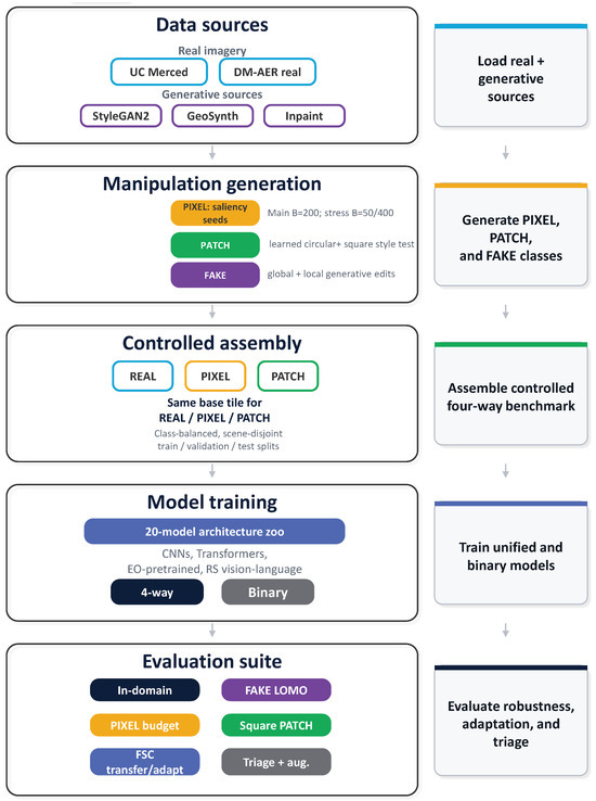
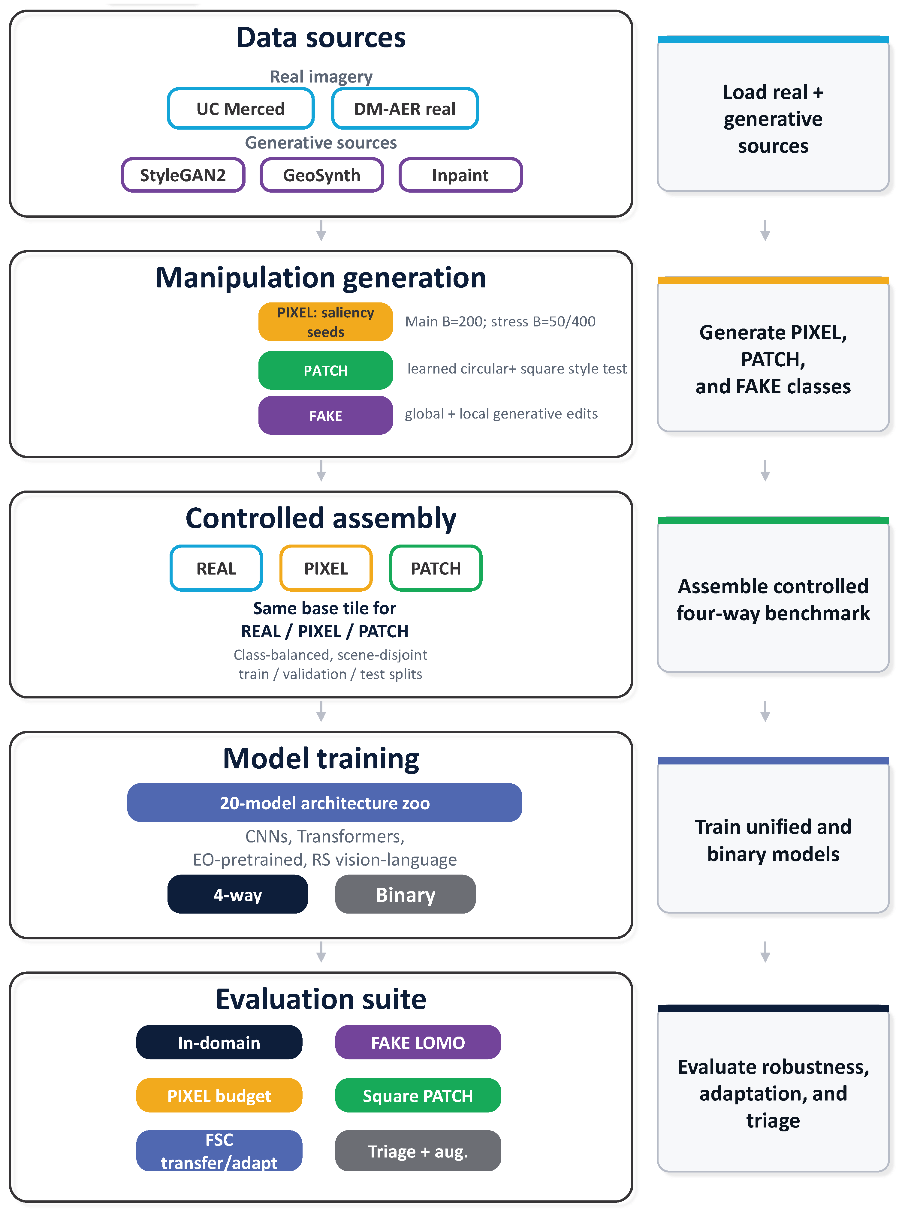
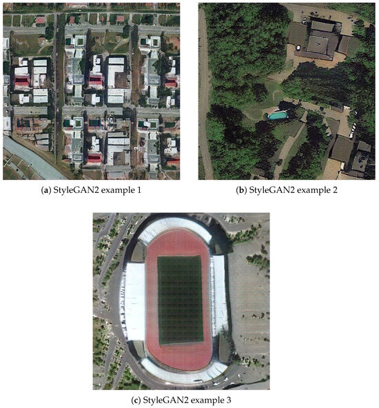
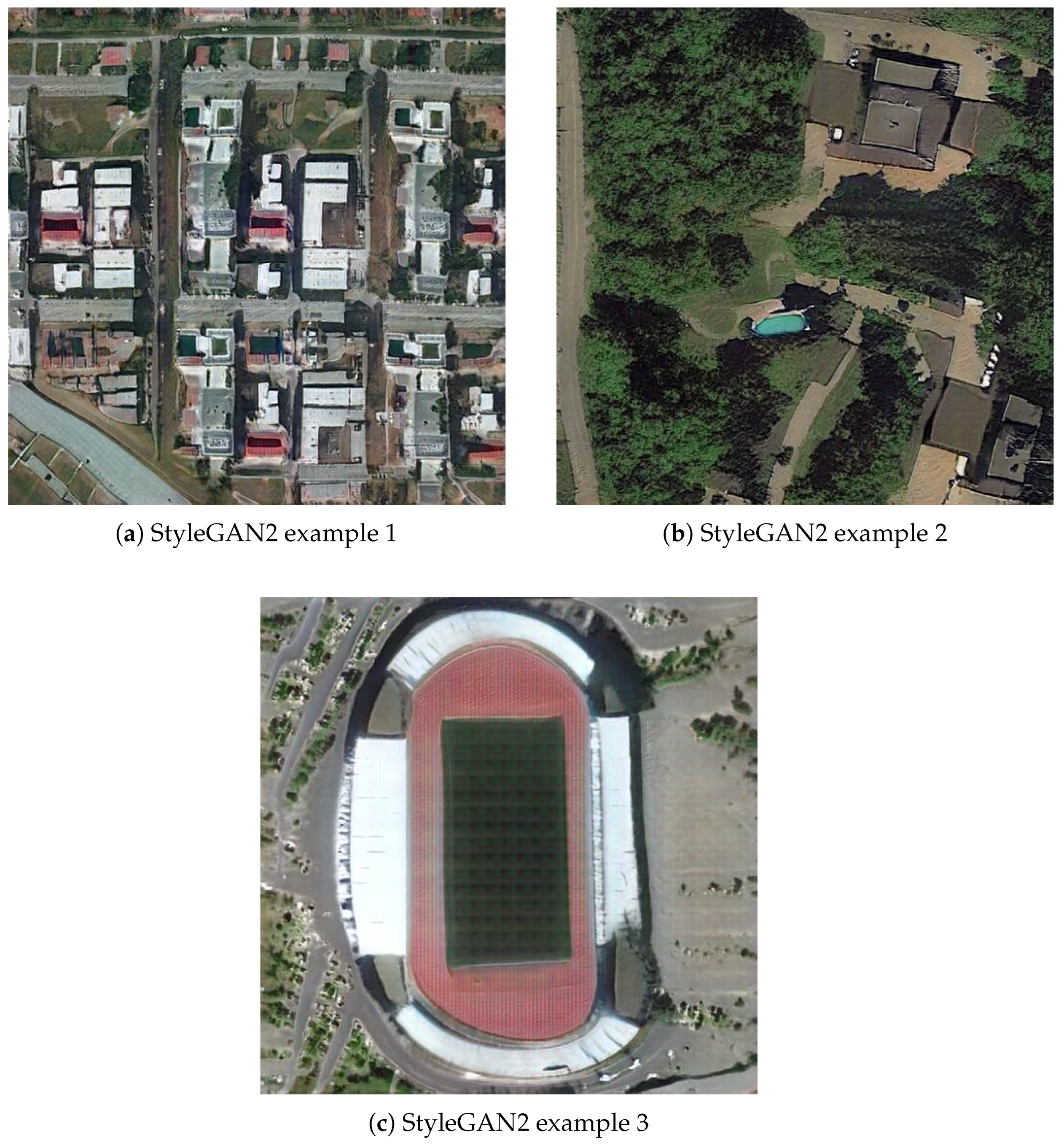
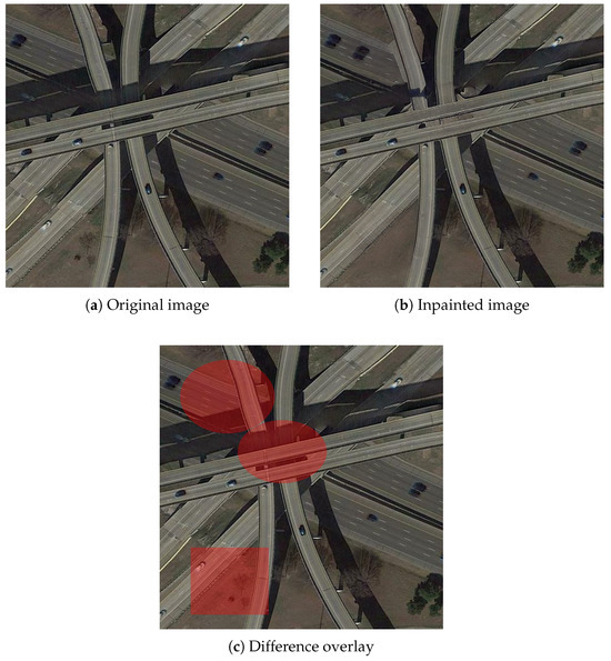
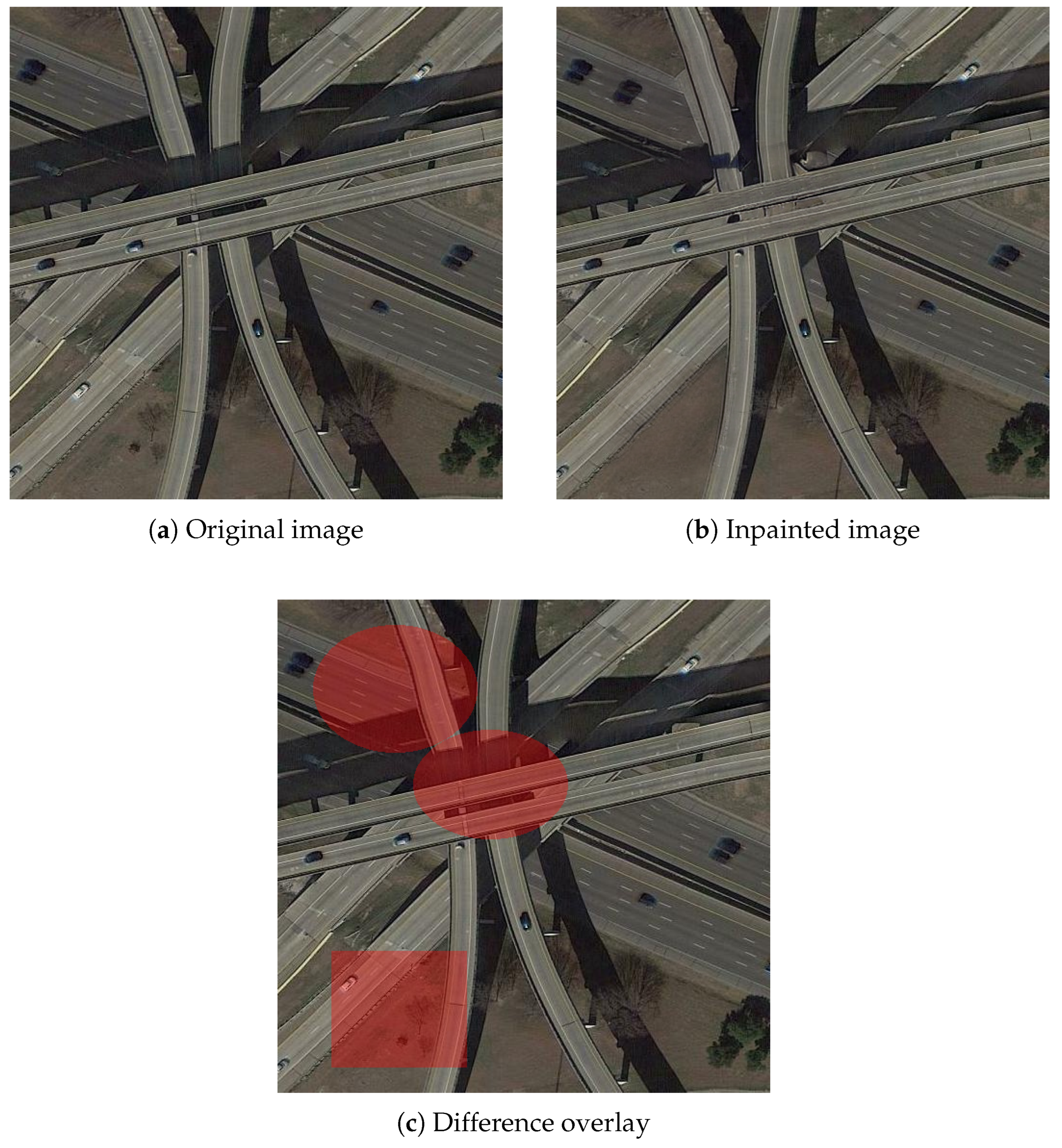
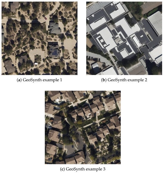
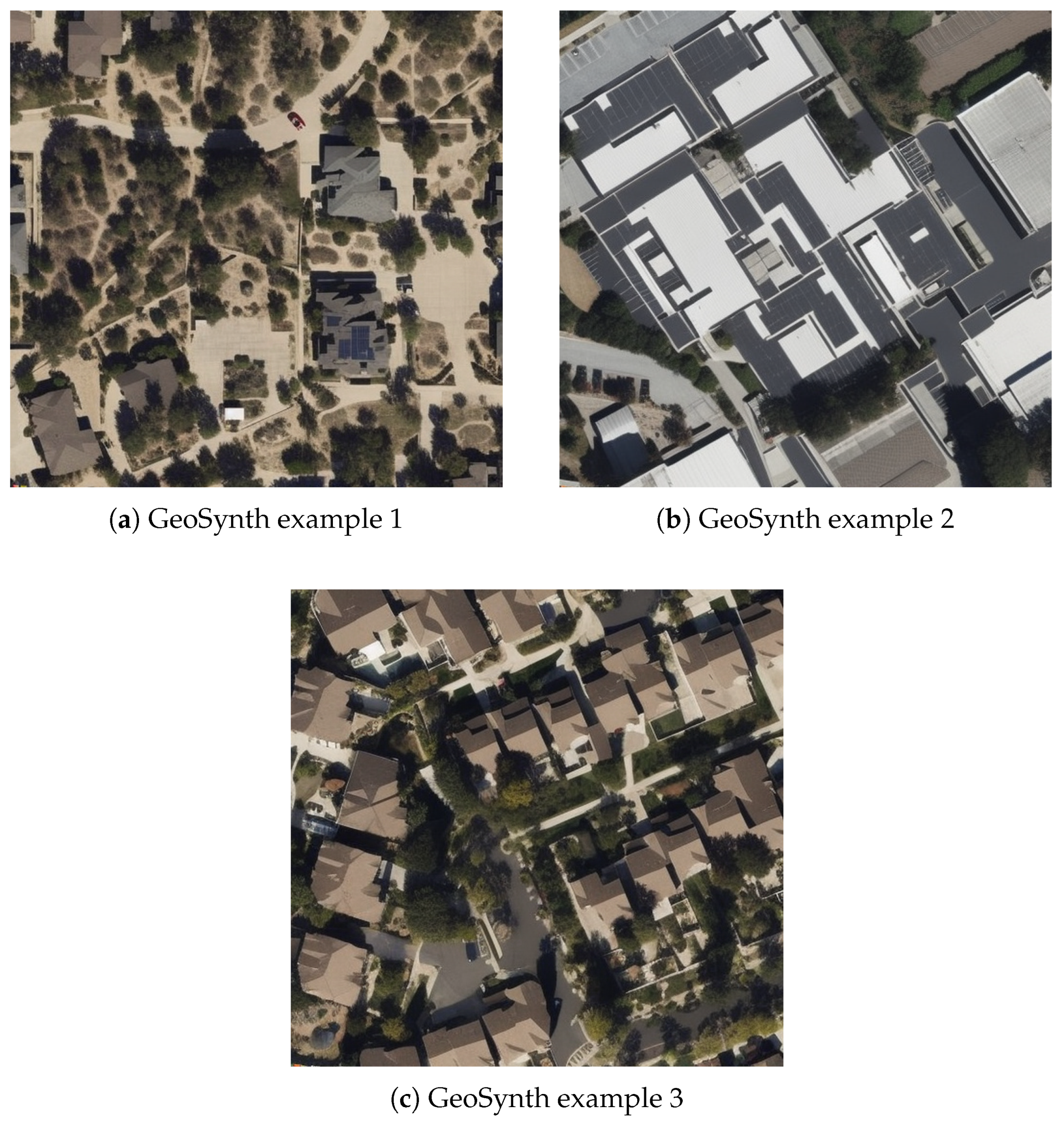
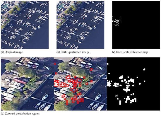
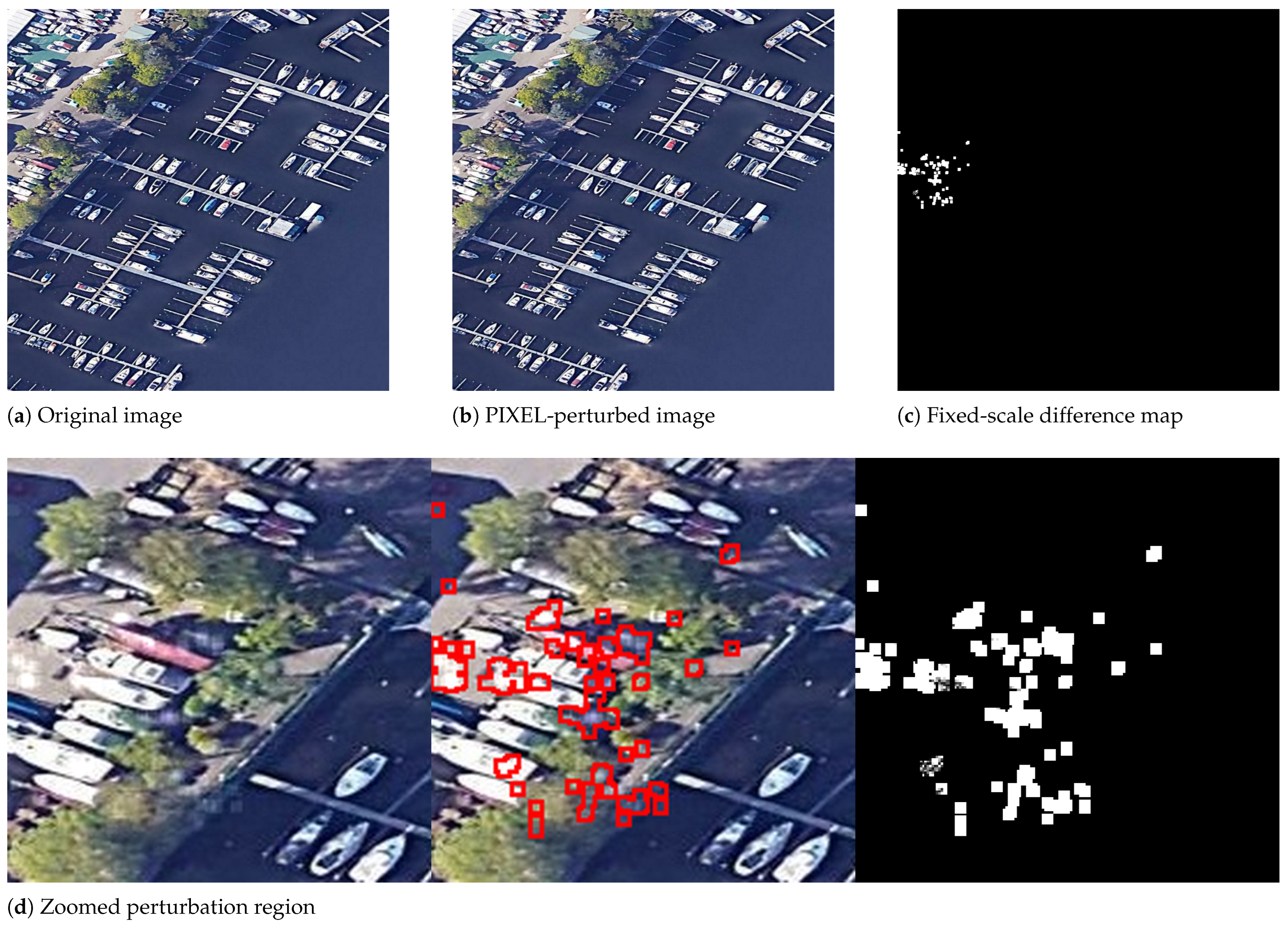
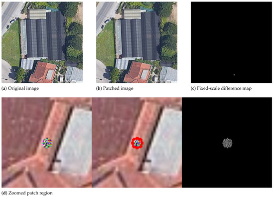
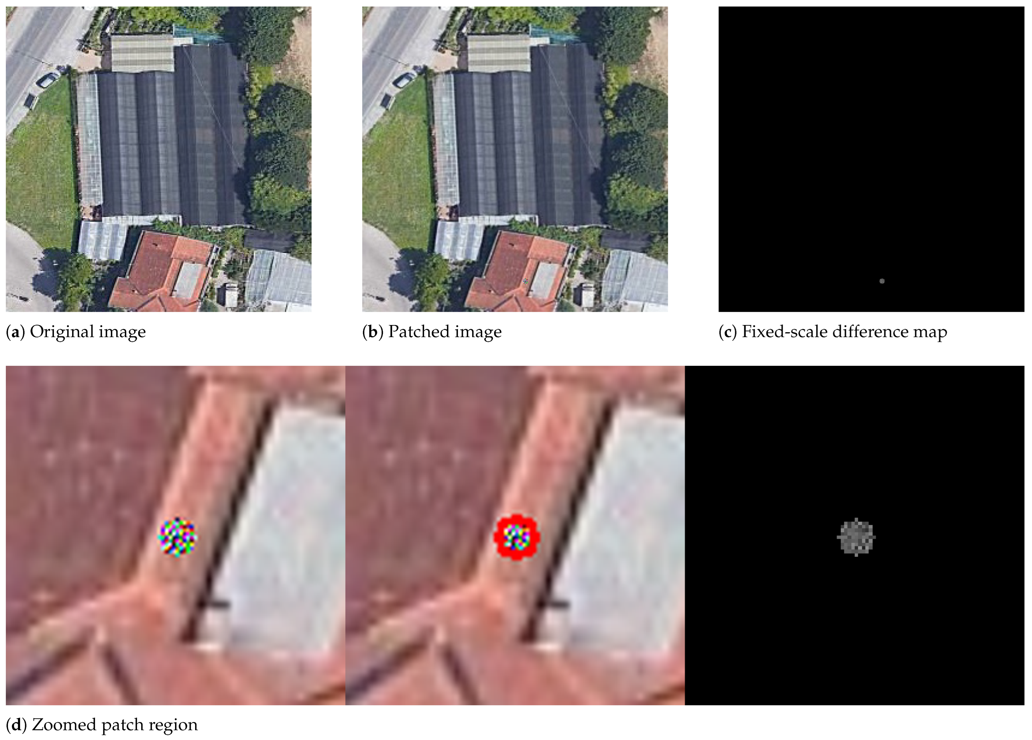
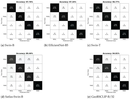
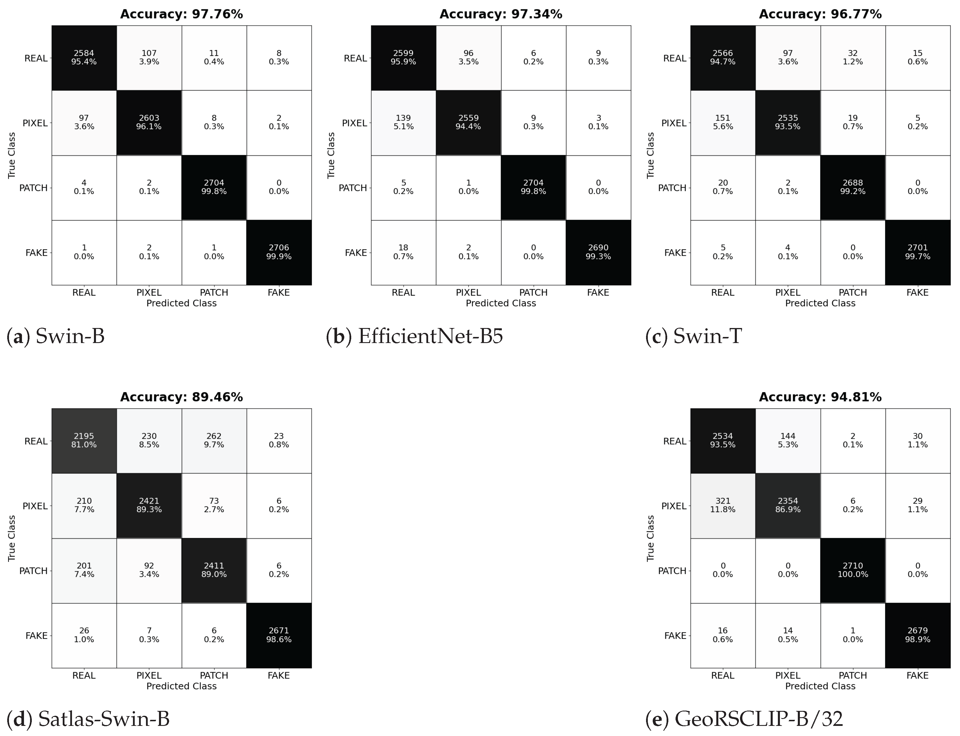
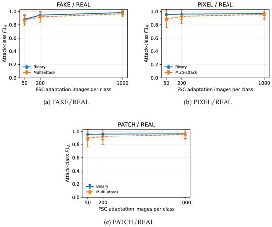
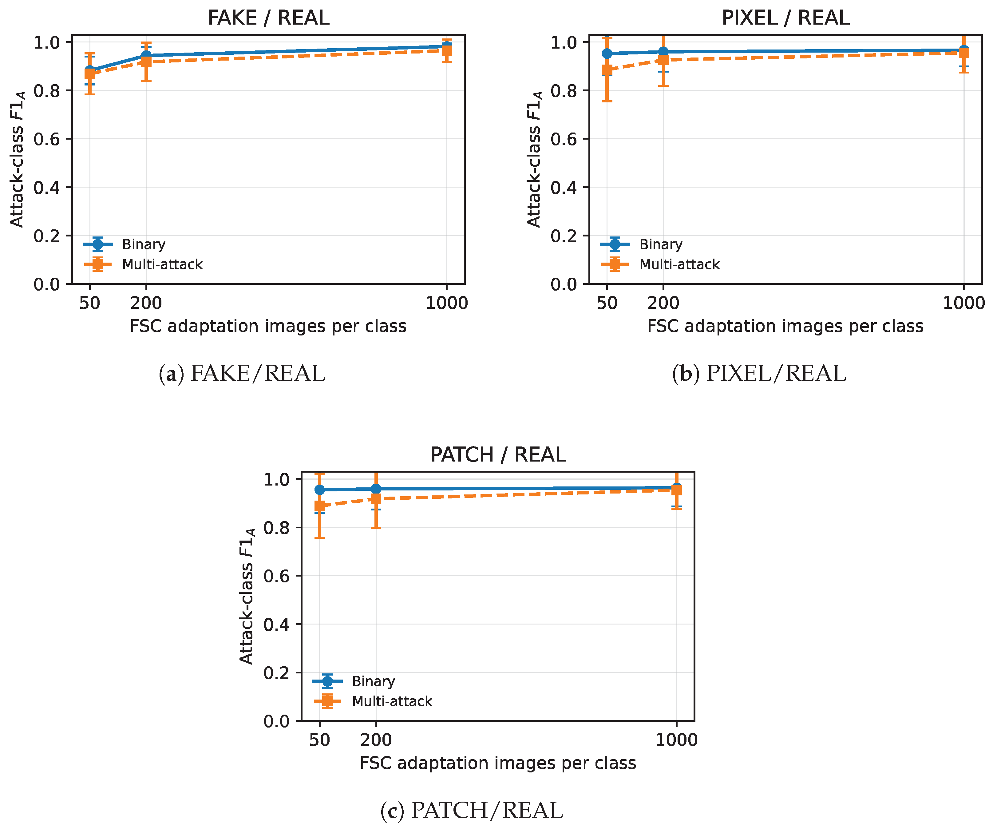

Disclaimer/Publisher’s Note: The statements, opinions and data contained in all publications are solely those of the individual author(s) and contributor(s) and not of MDPI and/or the editor(s). MDPI and/or the editor(s) disclaim responsibility for any injury to people or property resulting from any ideas, methods, instructions or products referred to in the content. |
© 2026 by the authors. Licensee MDPI, Basel, Switzerland. This article is an open access article distributed under the terms and conditions of the Creative Commons Attribution (CC BY) license.