1. Introduction
Agricultural systems are particularly vulnerable to flood hazards due to their susceptibility to seasonal cycles and their exposure to low-lying floodplains. Flooding can result in the complete loss of crops [
1], long-term soil degradation [
2,
3], and decreased productivity [
4,
5] throughout the growing season. In addition to damaging crops, floods can also affect land ownership stability. Large-scale and smallholder farmers face different levels of exposure to flooding and have varying capacities for recovery [
6]. To develop effective risk management strategies and safeguard livelihoods, it is essential to understand how flooding affects agricultural land use over time and across different areas.
The Mississippi Watershed is the largest in North America. It drains 41% of the contiguous United States and two Canadian provinces. It is the third-longest river in the world, the sixth-largest in sediment yield, and the eighth-largest in discharge volume [
7,
8,
9]. Over the past 50 years, the Mississippi River has served as a major trade and commerce hub for the United States, a significant waste disposal site, a hydroelectric power source, and a crucial source of cooling and drinking water [
8,
9,
10,
11]. Nonetheless, the Mississippi River has a past of devastating floods, with the significant flood in 1927 leading to the establishment of a comprehensive flood management system. This system is made up of levees, upstream dams and reservoirs, as well as spillways such as the Bonnet Carré Spillway located near New Orleans, which channels excess water into Lake Pontchartrain and subsequently into the Gulf of Mexico [
12,
13,
14]. Flooding in the basin results from both natural hydrologic processes and human modification of the river system.
The 2019 Mississippi River Basin flood was one of the most severe and destructive hydrological events in recent U.S. history. It was found to be the longest-lasting flood since the 1927 Great Flood [
15]. The flooding along the Mississippi River system over the years is caused by a combination of natural and human-driven factors, with human modifications to the river system being the most significant contributors [
13]. Mississippi floods in 2008, 2011, and 2015–2019 highlighted storm sequences, heavy rainfall, saturated soil, and snowmelts from the Northern Great Plains influenced floods in the lower part of Mississippi [
14,
16,
17]. Munoz et al. [
13] and Pinter et al. [
18] revealed that while climate change and land use changes do play roles, the substantial increase in flood levels observed in Mississippi over the past 100 to 150 years is primarily due to river engineering. Specifically, wing dikes and levees have greatly altered the way rivers manage high-flow events.
According to Munoz et al. [
13], flooding from the Mississippi River has led to significant environmental degradation, including the loss of essential wetlands and changes in wildlife habitats. These floods create social hardships by displacing communities [
19] and increasing health risks due to insufficient access to clean water [
20]. Armstrong et al. [
21] reported that the floodwaters released from the Bonnet Carré Spillway in 2019 led to a toxic algal bloom. This bloom caused the closure of 25 Gulf Coast beaches, resulted in a dolphin mortality event, and contributed to the complete collapse of shellfisheries in several areas of the Western Mississippi Sound. Economically, the impact is severe, resulting in extensive agricultural damage, increased infrastructure repair costs, and heightened navigation expenses, all of which undermine regional trade and economic stability. For instance, in 2011, the flooding of the lower Mississippi River resulted in approximately
$3.2 billion in damages to agriculture and infrastructure [
12]. The 2019 Mississippi River Basin floods caused major disruptions to agricultural production [
22], resulting in farmers being unable to plant on millions of acres. This led to significant financial losses, amounting to billions of dollars, and a considerable amount of unshipped grain, estimated at billions of dollars [
23]. As of August 2019, John [
24] reported that an estimate of about 645,800 acres of land was prevented from being planted during the flood events in Mississippi State alone. Damages in the Mississippi and Missouri River valleys surpassed
$1 billion across agriculture, manufacturing, and transportation [
17].
The characterization of flood frequency and extent at high temporal and spatial resolutions has been enabled by advances in remote sensing and geospatial analytics [
25,
26]. These capabilities have been built upon in previous studies, which have used climate models [
27,
28,
29], satellite-derived remote sensing data [
30,
31,
32,
33], machine learning techniques [
34,
35,
36], hydrological models [
37,
38,
39,
40,
41,
42], and a combination of these diverse sources and techniques to model and map flood occurrences, frequency, susceptibility, and risk. Accurate flood mapping in the Mississippi Delta requires remote sensing approaches capable of capturing spatial and temporal inundation dynamics. Synthetic Aperture Radar (SAR) is widely used for flood monitoring because it can acquire data under all weather and illumination conditions [
43]. Operating both day and night, SAR is particularly valuable for detecting flooding in urban areas [
44]. Flooded surfaces typically exhibit low backscatter relative to surrounding terrain, enabling rapid delineation of inundation. However, accurately mapping floods remains challenging, especially at local scales. SAR-based flood delineation may lack spatial detail due to limitations in resolution and viewing geometry, particularly in areas with complex topography, dense vegetation, or built environments [
43]. In urban settings, interpretation of SAR signals is further complicated by building shadowing, multiple reflections (double-bounce), and signal interactions with flat roofs and windows, which can reduce mapping accuracy [
45]. To enhance reliability and accuracy, SAR data are often integrated with other datasets and remote sensing approaches [
43].
Despite the advantages of SAR, optical satellite imagery datasets remain valuable for mapping the extent of floods and monitoring changes in large flood plains, particularly when multi-temporal imagery is used to observe inundation patterns and their impact on land use [
46]. The integration of spatial data is recognized as an effective means of assessing flood risk distribution and aids the high-resolution reanalysis of past flood events [
47,
48]. Sentinel-2 multispectral imagery is especially suitable for flood mapping due to its high spatial resolution (10–20 m), frequent revisit time, and spectral capability to distinguish water, vegetation, and soil moisture. However, spectral indices alone may misclassify shadows, wet soils, and built-up areas. Therefore, following recent studies [
49,
50], this study adopts a multi-layer approach by integrating Sentinel-2 mosaics with spectral indices, topographic variables, and soil-related layers to improve inundation detection. This integration improves flood detection by combining water-sensitive spectral information with terrain and soil characteristics, thereby reducing classification errors and providing a reliable method for large-scale flood mapping.
Land ownership plays a critical role in shaping exposure, vulnerability, and recovery from floods [
51]. Patterns of land ownership influence how agricultural land is managed, the types of crops cultivated, and the financial capacity to withstand or adapt to repeated flood events [
52]. In the Mississippi River Basin, parcel size and tenure vary widely, ranging from small family-owned farms to large, corporate-owned commercial operations [
53]. These differences contribute to uneven distributions of risk, with some landowners experiencing recurrent losses while others remain relatively protected. Despite their importance, parcel-level ownership and tenure are often underutilized in flood impact studies, limiting our understanding of how floods reshape agricultural systems at the scale where decisions are made and adaptations occur.
Despite substantial progress in flood mapping through remote sensing, hydrological modeling, and geospatial analytics, several important research gaps remain. Previous studies [
27,
54,
55] have primarily focused on delineating flood extent, forecasting inundation, or assessing hazard susceptibility at regional scales, with limited attention to the temporal behavior of floods, such as persistence, recurrence, and duration at fine spatial resolutions. In agricultural floodplains, these temporal dynamics are critical because short-term widespread flooding and prolonged localized inundation can produce very different impacts on crops, infrastructure, and land productivity. In addition, relatively few studies have linked flood exposure to parcel-level land ownership and tenure patterns, even though ownership structure strongly influences management capacity, recovery potential, and access to mitigation resources. Crop-specific vulnerability is also insufficiently addressed, particularly in regions where multiple crops occupy landscapes with varying flood sensitivities. These gaps are especially important in the Mississippi Delta, where repeated flooding intersects with intensive agriculture and diverse landholding patterns. Addressing these limitations requires an integrated framework that combines flood dynamics, agricultural exposure, and land ownership characteristics to better support equitable and effective flood-risk management.
To address these gaps, this study develops an integrated geospatial framework to evaluate the 2019 Mississippi River Basin flood impacts in the Mississippi Delta using Sentinel-2 imagery, spectral indices, topographic variables, soil-related datasets, cadastral parcel information, and crop distribution data. The specific objectives of the study are to: (1) map flood extent, persistence, and recurrence at high spatial resolution for the January–August 2019 flood season; (2) quantify parcel-level flood exposure and examine how flood impacts vary among small, medium, and large agricultural land parcels; (3) estimate crop-specific agricultural losses and evaluate the temporal distribution of flood impacts across major crops, including soybeans, corn, cotton, rice, and wheat; and (4) identify spatial inequalities in socio-agricultural vulnerability by linking flood dynamics with land tenure and cultivated land intensity. By integrating flood dynamics, agricultural exposure, and ownership structure, this study provides a practical decision-support framework for flood mitigation, crop insurance prioritization, land-use planning, and resilience strategies in flood-prone agricultural landscapes.
2. Materials and Methods
2.1. Study Area
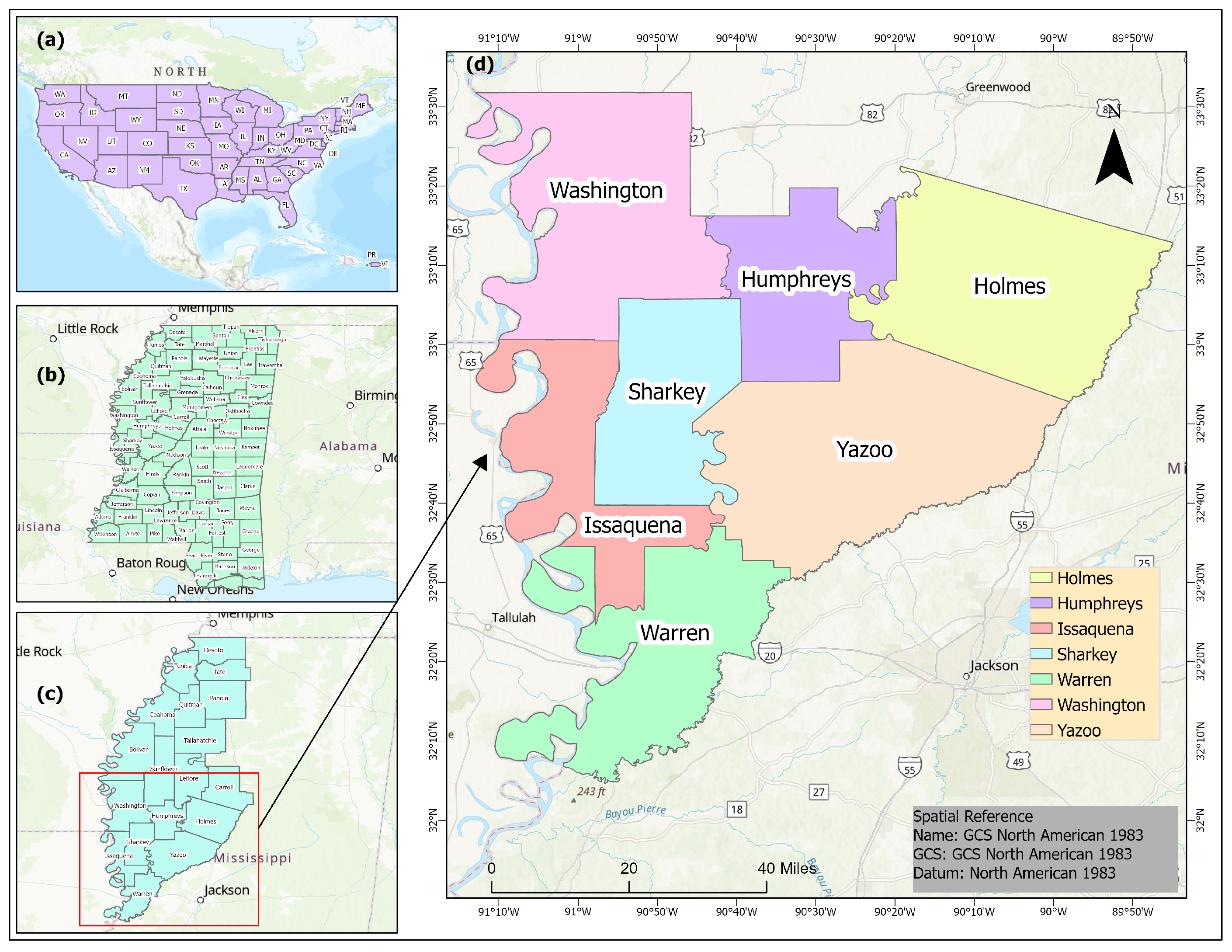
The study included 7 counties (
Figure 1): Washington County, Holmes County, Humphreys County, Sharkey County, Yazoo County, Issaquena County, and Warren County. These areas are located in the Yazoo–Mississippi Delta, often referred to as the Lower Delta, and form a distinct Alluvial plain in northwestern Mississippi bounded by the Mississippi and Yazoo Rivers [
56]. The Delta was historically a swampy area. It has been transformed through clearing, draining, and constructing levees for agricultural use [
57]. Characterized by flat topography [
58], fertile soils [
59], and extensive networks of rivers and tributaries [
60], the Yazoo–Mississippi Delta area is among the most agriculturally productive landscapes in the United States [
61]. The Delta’s subtropical climate, marked by warm summers and frequent rainfall, supports intensive cultivation of crops such as cotton, soybeans, rice, and corn [
62,
63].
2.2. Data Sources
This study used a combination of remotely sensed imagery and additional geospatial data to map flood frequency, evaluate agricultural losses, and analyze land tenure patterns in the study area as described in
Table 1.
2.3. Land Use Land Cover Mapping
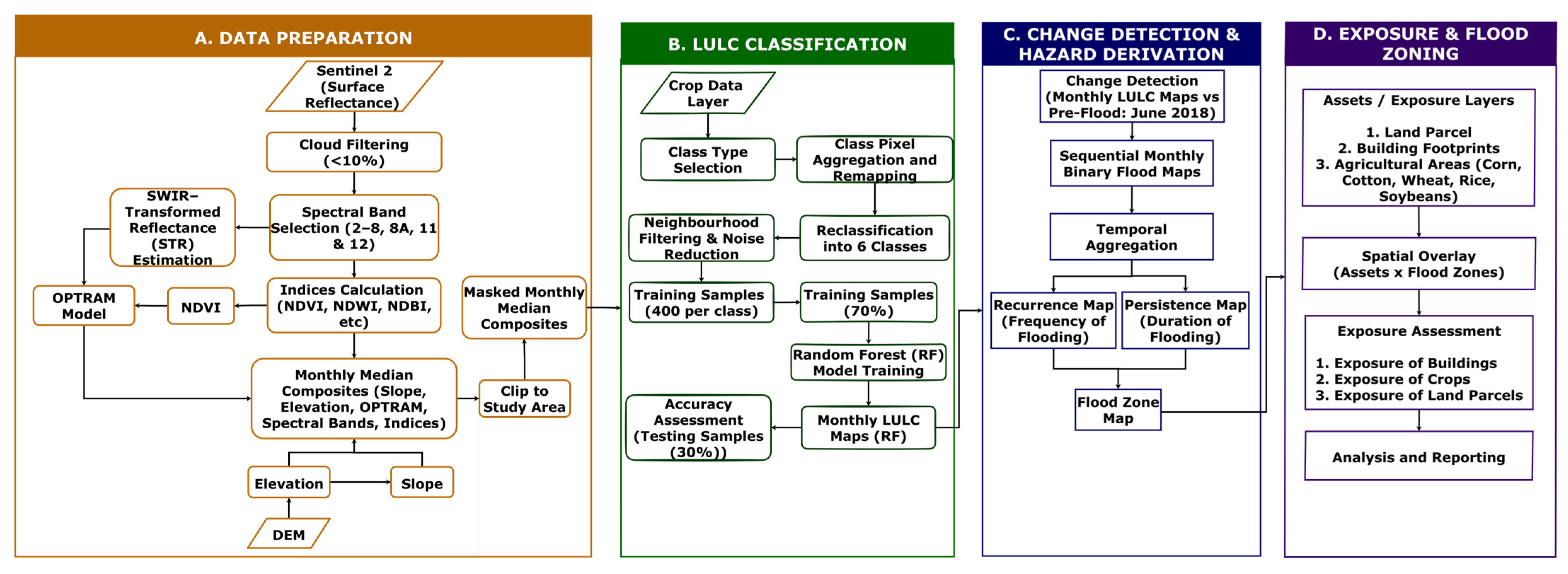
The methodological framework employed in this study is summarized in the flowchart (
Figure 2), which outlines the sequential steps for flood recurrence, persistence, and flood zone analysis, as well as infrastructure, crop land, and land parcel exposure assessment.
Sentinel-2 surface reflectance images (COPERNICUS/S2_SR) were accessed through Google Earth Engine (GEE) for the study period, filtered for <15% cloud cover within the study area. After atmospheric correction, cloud masking, and all spectral bands were scaled to surface reflectance values. Spectral indices were computed, including the Normalized Difference Vegetation Index (NDVI) [
64], Normalized Difference Water Index (NDWI) [
65], Normalized Difference Moisture Index (NDMI) [
66], Normalized Difference Built-up Index (NDBI) [
67], Automated Water Extraction Index (AWEI) [
68], Bare Soil Index (BSI) [
69], and Water Ratio Index (WRI) [
70]. These indices were included to improve class separability and enhance discrimination among land cover types. In addition, the Optical Trapezoid Model (OPTRAM) soil moisture index [
71,
72] was calculated using NDVI and shortwave infrared (SWIR) reflectance, following the methodology of [
72], with calibrated parameters. The OPTRAM-derived soil moisture layer was incorporated as an additional predictor variable, particularly to improve discrimination between the land cover classes. Topographic variables were incorporated to enhance classification performance. Elevation data were obtained from the USGS 3DEP Digital Elevation Model at 10 m spatial resolution. Slope layer was derived from the elevation dataset using terrain analysis functions (built-in ee.Terrain functions). Both elevation and slope were included as predictor variables in the classification process to account for terrain-driven variations in land cover distribution. A composite image was generated to include ten spectral bands (Blue, Green, Red, Red-edge bands, Near-Infrared, and Shortwave Infrared bands), slope, OPTRAM, spectral indices, and elevation at 10 m spatial resolution.
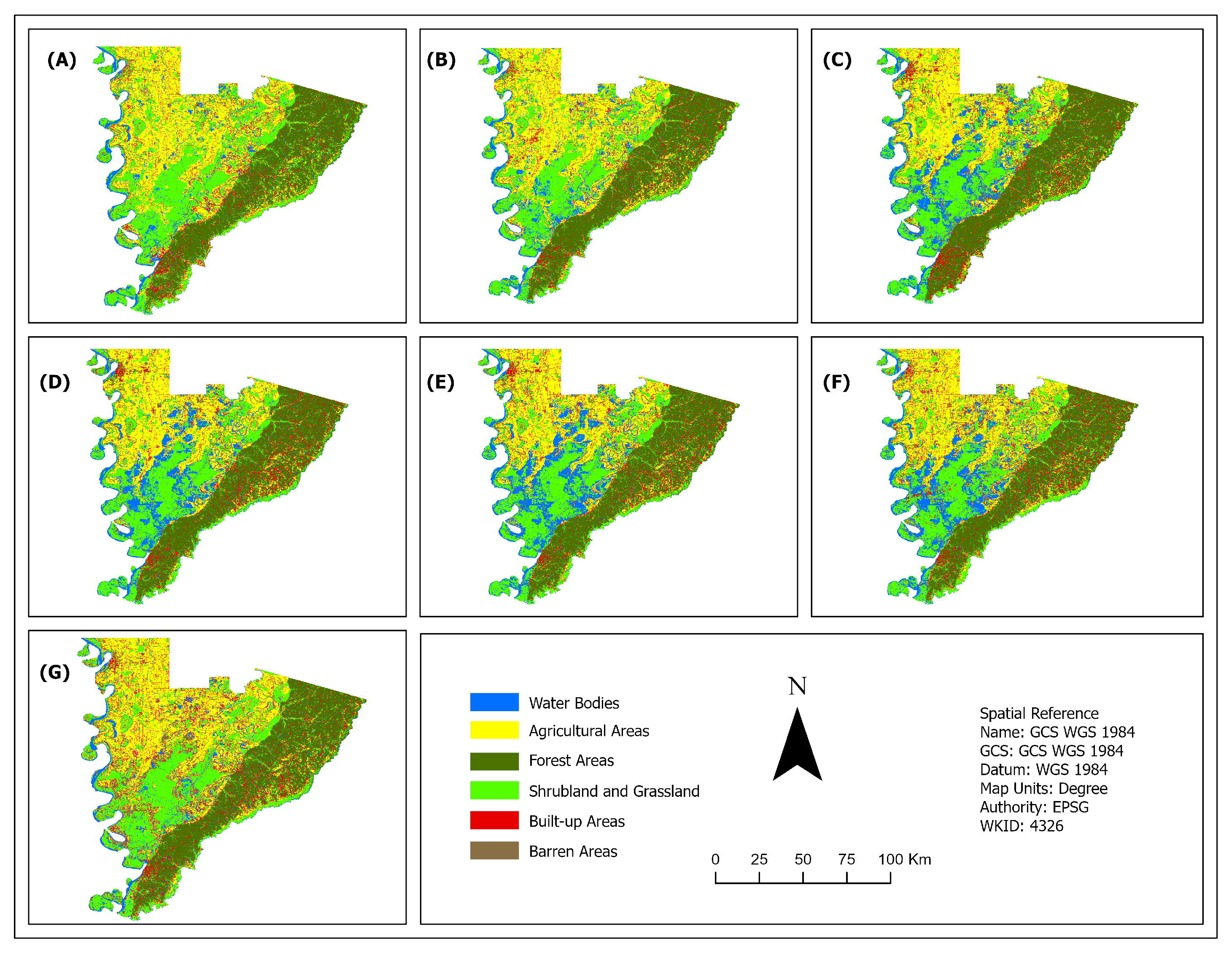
The 2018 and 2019 Cropland Data Layers (CDLs) from USDA-NASS were obtained at 30 m resolution and clipped to the study area. CDL crop codes were reclassified into six thematic classes (
Table 2): Water Bodies, Agriculture, Forest, Shrubs/Grassland, Built-up, and Barren. To improve the reliability of training data and reduce noise, a spatial homogeneity filtering approach was applied. A 3 × 3 majority neighborhood-based mode filter was applied, followed by a connected pixel filter to retain only homogeneous regions with ≥50 connected pixels in the contiguous clusters. This generated “pure pixels” with at least 75% class purity, which were used as training samples following a similar methodology from Hao et al. [
73] and Tran et al. [
74]. This approach ensured the selection of spectrally pure training samples and minimized mixed-pixel effects, thereby improving accuracy. A stratified random sampling approach was employed to generate 2400 training samples (400 per class) to balance the representation across all six land cover categories. The spectral bands, spectral indices, OPTRAM soil moisture, elevation, and slope values were assigned to each sample region. The dataset was randomly split into training (70%) and testing (30%) subsets. The training subset was used to develop the classification model, while the validation subset was held out for independent accuracy assessment of the final classification.
Land cover classification was performed using the Random Forest algorithm implemented in GEE. To perform hyperparameter tuning, the 70% training subset was further partitioned into two groups: 80% for parameter tuning (model fitting) and 20% for internal validation. A grid search hyperparameter tuning was carried out using the 80% subset training sample by testing multiple combinations of the number of trees (100–500) and the number of variables per split (mtry: 1–7). The optimal configuration was identified as 400 trees and mtry = 7, based on accuracy and Cohen’s Kappa using the 20% subset training sample. The final classifier was applied to the final composite image to generate the final land cover map at 10 m spatial resolution.
The classification was validated using the 30% test dataset. A confusion matrix was generated to compute Overall Accuracy (OA), Producer’s Accuracy (PA), User’s Accuracy (UA), and Cohen’s Kappa coefficient (κ), as explained in many studies [
75,
76,
77,
78,
79].
2.4. Change Detection and Flood Mapping
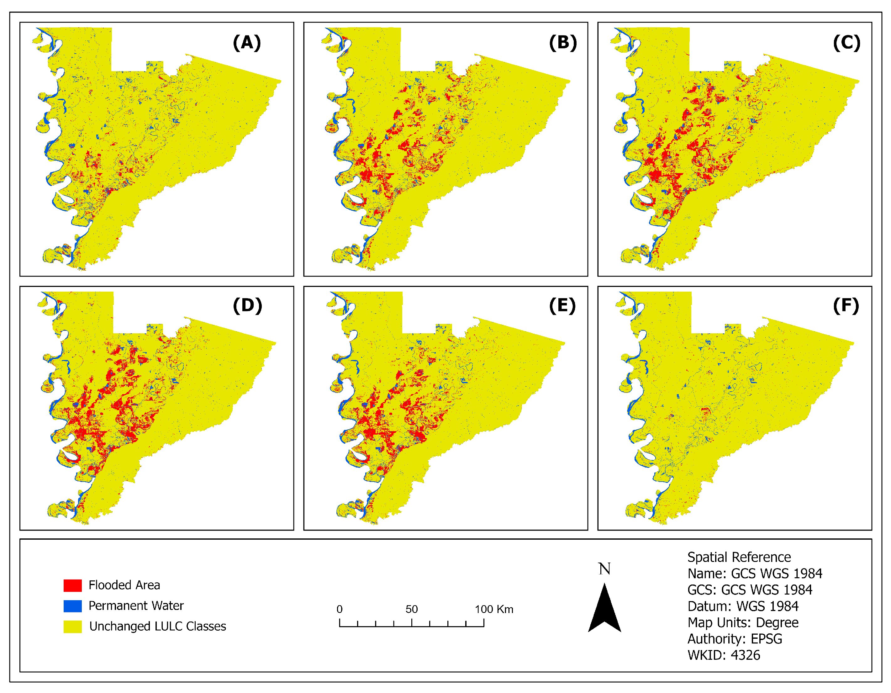
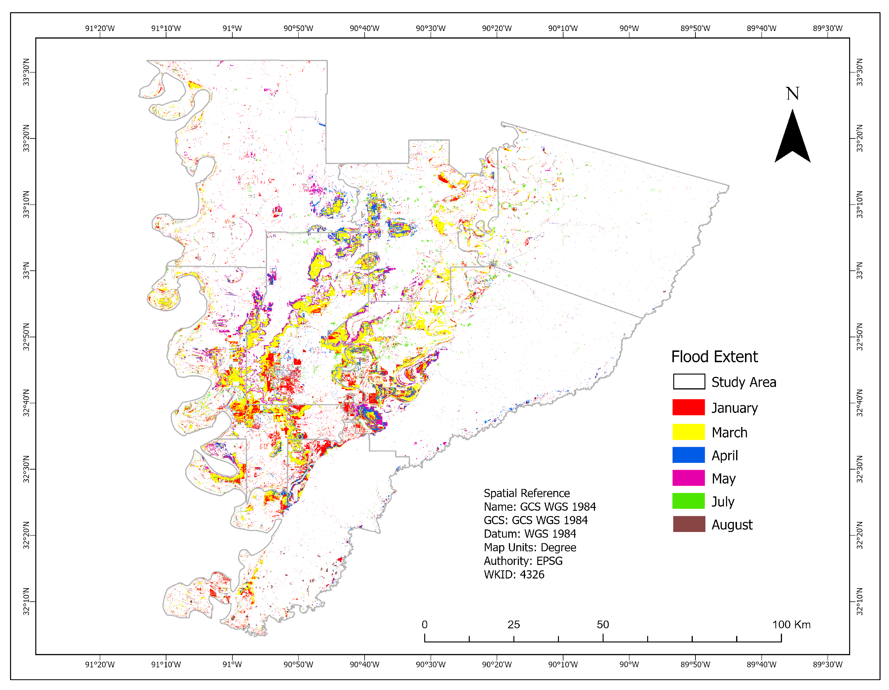
ArcGIS Pro 3.3 was used to perform a post-classification change detection between the pre-flood reference period (June 2018) and each flood month (January, March, April, May, July, and August 2019) to identify land–water transitions. A baseline permanent water mask was first generated using the USDA-NASS dataset and the June 2018 classification, representing persistent water bodies such as the Mississippi River, lakes, reservoirs, ponds, and streams. These permanent water features were excluded from subsequent analyses to prevent confusion with seasonal or inundation-related water dynamics. Flooded (inundated) areas were defined as pixels classified as non-water in the June 2018 reference image that transitioned to water in the corresponding 2019 flood-month image. Binary flood maps were generated for each time step (e.g., June 2018–January 2019, June 2018–March 2019, etc.), where inundation was identified as a change from non-water to water after masking permanent water bodies. Unchanged non-water areas and permanent water bodies were excluded from flood extent estimates to ensure that only newly inundated areas were mapped.
The accuracy of the change detection maps was evaluated using a post-classification comparison approach. Since change detection was derived from classified land cover maps, the reliability of change results depends on the accuracy of the individual classifications. Therefore, the classified maps used for change detection were first independently validated using a confusion matrix-based accuracy assessment as described in
Section 2.3.
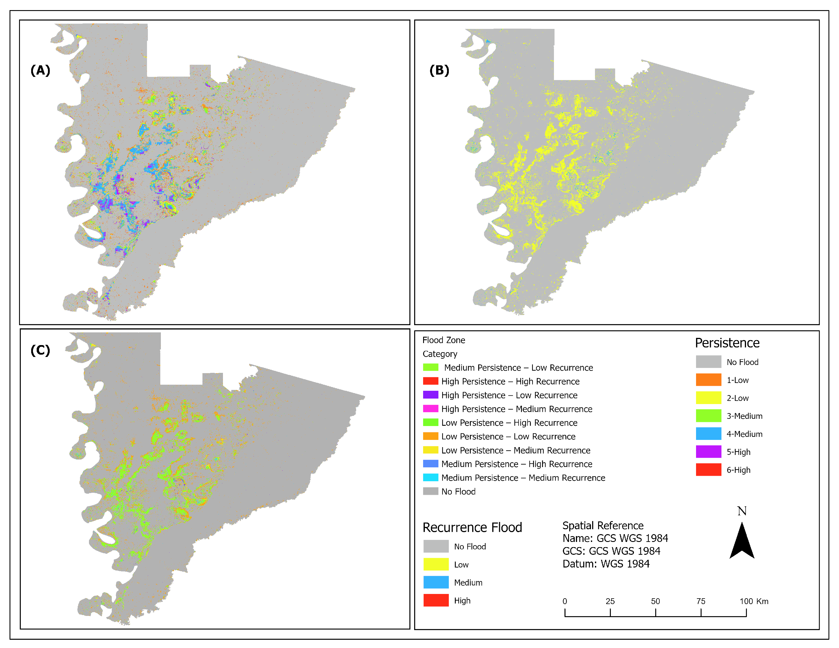
The monthly binary maps were combined using a raster calculation that summed the number of times each pixel was inundated over the study period. The resulting map showed flood frequency; higher values indicated pixels that were repeatedly inundated. To assess flooding persistence, a water inundation frequency (WIF) [
80] approach was adopted, in which the inundation frequency for each pixel was normalized to the total duration of the study period (6 months). WIF was computed as
where N
f represents the number of months in which a pixel was classified as flooded, and N
t is the total number of months in the observation period.
Based on the computed WIF values, the flooding persistence map was reclassified into four categories: non-flooded, low persistence, medium persistence, and high persistence. Pixels with no flooding (0% WIF) were categorized as 0 (non-flooded area). Pixels with WIF values ranging from 16.7% to 33.3% (1–2 months of inundation) were classified as having low persistence. WIF values defined medium persistence between 50.0% and 66.7% (3–4 months of inundation). High persistence included pixels with WIF values exceeding 83.3% (5–6 months of inundation).
Flood recurrence was evaluated by generating binary flood maps for each pair of consecutive months (January–March, March–April, April–May, May–July, and July–August). Transitions from non-flooded to flooded states were recorded as recurrence events. The binary transition maps were summed to calculate the total number of flood occurrences per pixel across all monthly intervals. The resulting map reflected the frequency of flood recurrence, indicating how often new flooding occurred over previously dry areas. Finally, the cumulative recurrence raster was reclassified into three levels: low, medium, and high. These levels represent areas with one, two, and three or more instances of flood recurrence, respectively.
Finally, a composite Flood Zone Map was generated by integrating both persistence and recurrence classes to represent combined flood dynamics. Pixels identified as non-flooded in either map were assigned to the “no flood” category. All other pixels were classified based on the combined influence of their persistence and recurrence levels. This integration differentiated flood zones into multiple classes that reflect varying degrees of flood hazard severity. Areas with high persistence and recurrence were interpreted as zones of extreme flood risk, and areas with low persistence and recurrence were interpreted as regions of occasional or short-term inundation.
To further refine the analysis, additional datasets were integrated, including built-up area polygons from Mississippi Automated Resource Information system (MARIS), land parcel data containing proprietary information (owner name, cultivated and uncultivated area, total parcel size), and the 2019 CDL from NASS to identify crops adversely affected by flooding (Rice, Corn, Winter Wheat, Soybean, and Cotton). The impact of flooding on land parcels was quantified using spatial analysis tools, including zonal statistics, frequency, summary statistics, and tabulate area in ArcGIS Pro (version 3.3). Land parcels intersecting flooded zones were classified based on their areal extent (hectares) to examine how flooding impacts vary across different parcel sizes. Parcel size classification was performed using the Jenks Natural Breaks (optimization) method, which determines class intervals by minimizing variance within classes and maximizing variance between classes. This data-driven approach identifies natural groupings inherent in the parcel size distribution. Based on the resulting thresholds, parcels were categorized into three classes: small (≤48 ha), moderate (48–112 ha), and large (>112 ha). These classes represent statistically derived groupings of parcel sizes and are independent of flood exposure. Following classification, spatial analysis was conducted for each tenure category to determine the distribution of flooded cultivated and flooded areas across the flood zones.
5. Conclusions
This study demonstrates that the impacts of the 2019 Mississippi River Basin floods were driven more by spatial extent and timing of short-duration flooding than by prolonged inundation alone. Low-persistence, low-recurrence floods accounted for the majority of crop and infrastructure exposure, highlighting the significant role of infrequent but widespread flood events in shaping agricultural risk. In contrast, high-persistence flooding, although spatially limited, represents areas of chronic vulnerability with potential long-term impacts on infrastructure integrity and land usability.
The results further reveal that parcel size influences flood vulnerability, with small agricultural parcels consistently exhibiting higher proportional exposure and cultivated land intensity across flood categories. This suggests that flood risk is not only a function of hydrologic processes but is also shaped by land ownership patterns and the spatial distribution of agricultural activities.
By integrating flood persistence and recurrence with parcel-level and crop-specific analyses, this study provides a more comprehensive framework for assessing agricultural flood risk. The findings highlight the importance of incorporating both flood duration and frequency into risk assessments, particularly identifying areas exposed to large-scale, short-term flooding events that may otherwise be underestimated.
From a management perspective, the results highlight the need for targeted flood mitigation strategies that prioritize highly exposed agricultural zones, especially those dominated by smaller parcels. Integrating flood dynamics with land ownership and infrastructure data can support more effective planning, insurance allocation, and resilience-building efforts across the Mississippi River Basin.