Article

Dual-Branch Deep Learning for Forest Stand Classification in Hainan Tropical Rainforests with Multi-Source Remote Sensing Data

1
Key Laboratory of Earth Observation of Hainan Province, Hainan Aerospace Information Research Institute, Wenchang 571300, China
2
Aerospace Information Research Institute, Chinese Academy of Sciences (AIRCAS), Beijing 100094, China
3
College of Mathematics and System Sciences, Xinjiang University, Urumqi 830046, China
4
School of Artificial Intelligence, China University of Geosciences (Beijing), Beijing 100094, China
*
Author to whom correspondence should be addressed.
Remote Sens. 2026, 18(12), 2001; https://doi.org/10.3390/rs18122001
Submission received: 11 April 2026 / Revised: 4 June 2026 / Accepted: 11 June 2026 / Published: 16 June 2026

Highlights

What are the main findings?
  • DB-FFN model.
  • Effectiveness of multi-temporal information.
  • Effectiveness of multi-source data fusion.
What are the implications of the main findings?
  • Improvement in tree species classification accuracy.
  • Forest stand species classification mapping of the study area.

Abstract

Tropical rainforests are characterized by high species diversity and complex canopy structure, making accurate forest stand classification important for ecosystem assessment, biodiversity monitoring, and forest carbon estimation. However, single-source remote sensing data lacks sufficient discrimination ability to address the issue of spectral similarity among classes, and conventional convolutional neural networks often struggle to extract discriminative features and integrate heterogeneous data in highly complex forests. To address these challenges, this study developed a dual-branch deep learning framework that integrates DenseNet and ConvNeXt for classification in Hainan Tropical Rainforest National Park. The framework combines sub-meter Google Earth imagery to capture spatial–textural detail with multi-temporal Sentinel-2 imagery to represent phenological variation. The results showed that multi-temporal Sentinel-2 data outperformed single-date imagery by capturing phenological patterns, and that the fusion of high-resolution spatial information and multi-temporal spectral information yielded higher accuracy than either data source alone. The dual-branch model achieved an overall accuracy of 94.47% and a Kappa coefficient of 0.94, outperforming all benchmark models. These findings indicate that branch-specific feature extraction and adaptive fusion can improve fine-scale classification in complex tropical rainforest environments. The proposed framework provides a practical approach for fine-scale forest stand mapping and may support biodiversity monitoring, ecological assessment, and sustainable forest management.

1. Introduction

Forests are the primary part of terrestrial ecosystems. They help maintain the global carbon balance, protect biodiversity, and regulating regional climate [1,2]. Tropical rainforests cover only about 6% of the Earth’s land area. Yet they contain more than half of all known species and hold roughly 25% of the carbon stored in terrestrial vegetation. This role makes them essential to global ecological security [3]. Hainan Tropical Rainforest National Park is China’s most concentrated and best-preserved tropical rainforest region. It is both a global biodiversity hotspot [4] and a strategic site for national ecological construction. The condition of its forest ecosystem directly affects water conservation and carbon storage. Fine-scale forest stand identification and mapping are therefore necessary for biodiversity monitoring, accurate carbon accounting, and sustainable ecosystem management [5]. However, the tree species composition and spatial structure of Hainan’s tropical rainforest are complex. Native species such as Dacrydium pectinatum and Podocarpus imbricatus form multi-layered and uneven-aged stands. By contrast, plantation forests such as rubber and eucalyptus usually show a more uniform pattern. Secondary forests at different successional stages are also mixed across the landscape. This heterogeneity makes forest stand classification difficulty in this region.
Traditional forest resource inventories rely on manual ground surveys. Although accurate, they are inefficient, have limited coverage, and struggle to meet modern demands for large-scale, high-frequency, and fine-grained monitoring. Remote sensing is now the main approach for studying forest vegetation types. Remote sensing data acquired via airborne and satellite platforms provide an essential foundation for forest tree species classification research. Early studies primarily relied on medium-to-low-resolution imagery such as MODIS and Landsat. While offering broad coverage, these data are constrained by the mixed-pixel problem, making fine tree species identification difficult [6]. Recent advances in remote sensing have improved both the efficiency and precision of forest tree species classification [7,8]. Remote sensing data commonly used in this field mainly include airborne LiDAR data, airborne hyperspectral data, and high-resolution multispectral data. Airborne LiDAR emits laser pulses and records reflected signals to generate point clouds. LiDAR data contain forest height and structural information, which are helpful for improving classification accuracy [9]. Airborne hyperspectral data cover a broad spectral range from visible to thermal infrared. Their high spectral and spatial resolution can increase both the number of species that can be identified and the accuracy of classification. Still, LiDAR and airborne hyperspectral data are expensive to acquire, cover limited areas, and depend on flight plans and weather conditions, which restrict their use for large-scale, continuous monitoring needs [10]. Satellite imagery has also improved in spatial resolution. For instance, the panchromatic resolution of WorldView-2/3 data can reach 0.46 m and 0.31 m, respectively, and high-resolution imagery on the Google Earth platform can reach up to 0.3 m. These data provide a practical basis for large-scale tree species classification. For example, Fang et al. used WorldView-3 imagery to classify street trees in Washington, achieving an accuracy of 73.7% [11]; Sun et al. combined WorldView-2 data with LiDAR data for tree species classification in a wetland park, achieving an overall accuracy of 89% [12]; Lei et al. used Google Earth imagery for individual tree species classification, achieving a maximum overall accuracy of 92.48% [13].
The complex vegetation structure and high species diversity of tropical rainforests often cause different species to show similar spectral responses in remote sensing classification. This problem of “different objects with similar spectra” remains a major obstacle to accurate species identification. Heterogeneous canopy conditions can produce highly similar spectral signatures among different tree species, which makes discrimination from single-date remote sensing imagery difficult [14]. Studies have shown that multi-temporal remote sensing imagery can reduce this difficulty and improve classification accuracy in complex forest environments [15,16]. Multi-temporal data capture spectral variation across different phenological stages and provide time-dependent information for species discrimination. Grabska et al. used Sentinel-2 time-series data from 2018 to classify tree species in the mixed forests of the Polish Carpathian Mountains. Their results showed that time-series imagery improved overall mapping accuracy by about 5% to 10% compared with single-date imagery [17]. Hill et al. used five multi-temporal airborne multispectral images and found that the combination of growing-season and leaf-off imagery was the most effective for species discrimination [18]. Fang et al. classified street trees with 12 WorldView-3 images acquired from April to November and achieved an overall accuracy of 73.7%. They also reported that the autumn senescence period provided the most useful phenological information for classification [11].
Among the currently available satellite data sources, Sentinel-2 is well suited to large-scale forest tree species classification and mapping. The European Space Agency provides Sentinel-2 data free of charge, and its core spatial resolution is 10 m. Its revisit interval of 3 to 5 days allows repeated observation of vegetation across different phenological stages. Multi-temporal datasets built from key phenological periods can therefore reveal temporal patterns in vegetation spectra and provide strong support for tree species discrimination in tropical rainforests [19,20].
Existing studies have also shown that combining multi-temporal data with high-resolution imagery can further improve the accuracy of forest tree species classification. Neyns et al. used multi-temporal PlanetScope data together with high-resolution aerial imagery and found that this combination produced the best result, with an overall accuracy of 0.88 [21]. Daryaei et al. reported that multi-temporal Sentinel-2 data significantly improved classification accuracy, and that the addition of 3 m PlanetScope imagery led to further gains [22]. Eskandari et al. combined Sentinel-2 data, field samples, and 0.65 m Google Earth imagery for land cover classification, and their results showed the value of Sentinel-2 data and high-resolution Google Earth imagery for this task [23]. Sub-meter Google Earth imagery can represent canopy texture, crown shape, and spatial pattern in fine detail [24]. This complementarity suggests that combining time-series Sentinel-2 data with sub-meter Google Earth imagery may improve tree species identification in complex tropical forest scenes.
Classification performance also depends on the analytical method. Traditional machine learning methods such as Random Forest (RF) and Support Vector Machine (SVM) often show clear limits when they are applied to large, high-dimensional, and multi-source remote sensing datasets. These methods usually depend on manually designed features. Their level of automation and adaptability is therefore limited, which can restrict further gains in classification performance. Since 2015, deep learning methods, especially Convolutional Neural Networks (CNNs), have become a main approach in remote sensing image classification because they support automatic feature extraction and end-to-end learning [25,26]. Common CNN models used in tree species classification include VGG [27], GoogLeNet [28], ResNet [29], and DenseNet [30] (Huang et al., 2017). Guo et al. compared three CNN models with WorldView-3 and Google Earth imagery and found that DenseNet extracted features more effectively and achieved the best accuracy in individual tree species classification [31]. Rezaee et al. used VGG-16 with WorldView-3 data and reported a classification accuracy of 92.13%, which was much higher than that of Random Forest and Gradient Boosting methods [32]. Zou et al. combined LiDAR-derived three-dimensional tree information with a Deep Belief Network (DBN) and achieved a classification accuracy of 95.6% [33]. Raczko et al. compared Artificial Neural Networks, SVM, and RF for tree species classification. Their results showed that the Artificial Neural Network performed best, with a classification accuracy of 77% [34]. Chen et al. used Res-UNet for individual tree species classification on WorldView-3 imagery acquired in March 2019 in Huangshan, Anhui Province, China. They reported an overall accuracy of 94.29%, which was higher than that of U-Net and ResNet [35]. More recent models, such as EfficientNet [36], ConvNeXt [37], and Vision Transformer [38], have further improved image classification performance. Huang et al., in a study based on drone imagery from Dongtai Forest Farm, also pointed to the potential of ConvNeXt and Transformer models for forest tree species classification [39]. These studies show that deep learning methods, especially CNN-based models, have made substantial progress in tree species classification.
As multi-source remote sensing data are used more widely in tree species classification, effective fusion of different image types has become a key issue for improving classification accuracy [40,41]. Existing studies that use high-resolution imagery together with multi-temporal spectral data still often rely on a single network for feature extraction or on simple fusion at the decision level [42,43]. In practice, a single network architecture often cannot extract and fuse these data effectively. High-resolution imagery mainly provides two-dimensional spatial structure, whereas multi-temporal spectral data mainly reflect one-dimensional temporal dynamics [44,45,46]. These two data types differ substantially in the way that information is represented. A single network therefore has difficulty adapting to both. Simple concatenation or early fusion can also suppress important features or create an imbalance between modalities, which may reduce classification performance [47]. To address this issue, dual-branch and multi-branch architectures have received increasing attention. Using the TreeSatAI dataset, Qin et al. proposed a multi-branch classification model for multi-source remote sensing data. Their model outperformed DenseNet121, ConvNeXt-Tiny, and ResNet-18 across performance metrics [48]. Huang et al. [49] proposed a Dual-Branch Attention-Aided Convolutional Neural Network (DBAA-CNN) for hyperspectral image classification. Their method outperformed 1D-CNN [50], 2D-CNN [51], 3D-CNN [52], and 3D-2D mixed CNN [53] in both classification accuracy and processing time. Zhu et al. proposed a dual-branch attention fusion network DBAF-Net with an adaptive sampling strategy to implement accurate multiresolution remote sensing image classification [54]. These studies suggest that branch-based architectures are better suited to heterogeneous data because each branch can adapt to a specific data type. This design can make fuller use of complementarity across modalities and improve tree species classification.
Against this background, this study focuses on the classification challenge created by complex species composition and the strong presence of “different objects with similar spectra” in the Hainan tropical rainforest. It uses sub-meter Google Earth imagery and multi-temporal Sentinel-2 imagery to examine whether the combination of high-resolution spatial information and multi-temporal spectral features can improve tropical rainforest tree species classification. To account for the difference between the two-dimensional spatial structure in high-resolution imagery and the one-dimensional temporal variation in multi-temporal spectra, this study develops a Dual-Branch Feature Fusion Network (DB-FFN). The spatial branch uses DenseNet-121 to learn the complex texture patterns in Google Earth imagery. The temporal branch uses ConvNeXt to extract long-range features from multi-temporal Sentinel-2 data. An adaptive fusion module is then used to integrate the two feature streams at a deeper level. The goal is to improve tree species classification accuracy under the complex conditions of the Hainan tropical rainforest and to provide technical support for biodiversity monitoring, carbon accounting, and sustainable ecosystem management.

2. Materials and Methods

2.1. Study Area

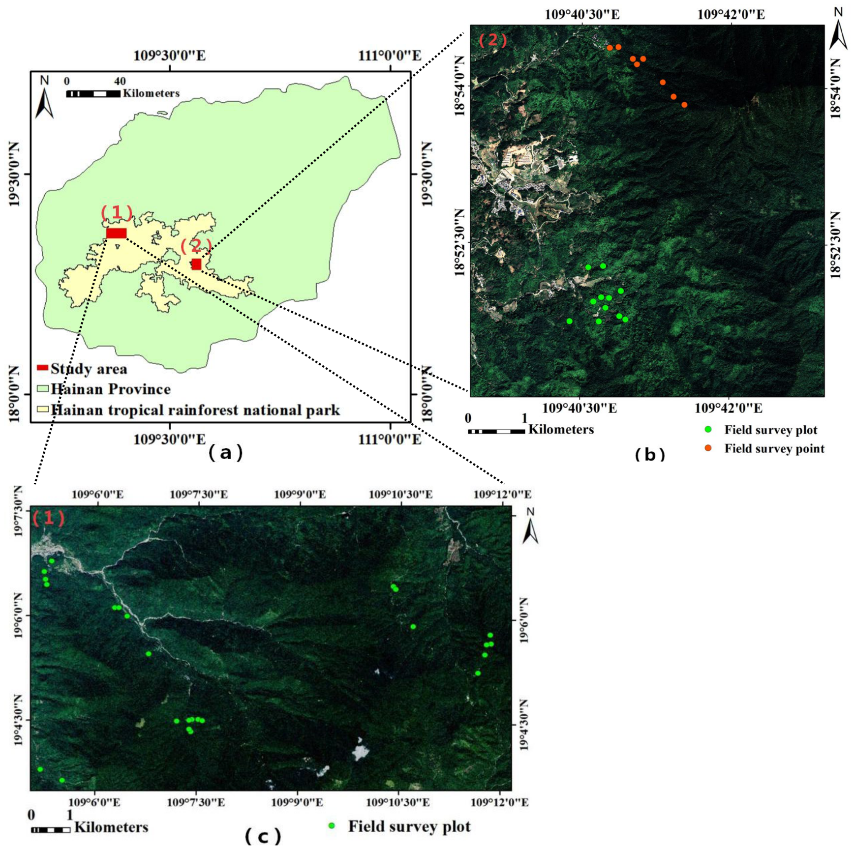
The study area is in Bawangling National Nature Reserve (109°02′–109°13′E, 19°02′–19°12′N) and Wuzhishan National Nature Reserve (109°32′–109°43′E, 18°48′–18°59′N), Hainan Province. Both are in the core zone of Hainan Tropical Rainforest National Park. Figure 1 shows its geographical location. The region has a typical tropical monsoon climate. The annual average temperature is 22–25 °C, and the annual precipitation is 1800–2200 mm. The rainy season is from May to October, making up more than 70% of the annual rainfall. The relative humidity in the forest is always high, usually between 84% and 90%.
The forest vegetation in this area has unique, diverse and complex structures. It is not only the only habitat for globally endangered species like the Hainan Gibbon, but also an important plant gene pool. Bawangling Reserve has recorded 2213 species of vascular plants, which shows its high botanical diversity [55,56]. The forest structure mainly consists of three interwoven forest types: first, tropical montane rainforests led by rare native tree species such as Dacrydium pectinatum and Podocarpus imbricatus. These include the “Wuzhi Sacred Tree”—a Dacrydium pectinatum over 2600 years old with a diameter at breast height (DBH) of 2.3 m; second, large-scale single-species plantations of economic trees such as rubber, eucalyptus, Pinus latteri, and Pinus caribaea; third, secondary forests at different recovery stages after human or natural disturbances. The mixed distribution of primary forests, plantations and secondary forests forms a dynamic and complex landscape influenced by both natural and human factors.

2.2. Data Acquisition and Preprocessing

2.2.1. Remote Sensing Data

This study uses Google Earth high-resolution imagery and multi-temporal Sentinel-2 satellite imagery for multi-source data joint analysis to capture the spatial structure and phenological characteristics of the study area.
(1)
High-Resolution imagery
This study uses two high-resolution images that cover the Bawangling and Wuzhishan study areas in Hainan Tropical Rainforest National Park. The images were taken on 12 November 2019, and 3 December 2021, with a spatial resolution of 0.56 m. They have three visible channels: red, green, and blue. The high-resolution imagery clearly shows crown morphology, texture, and spatial arrangement, and it is a key data source for distinguishing forest types and small differences between species.
(2)
Sentinel-2A/B imagery
The Sentinel-2A/B satellites are land surface monitoring satellites launched by the European Space Agency (ESA), including the 2A and 2B satellites. Their Multispectral Instrument (MSI) provides spectral information in 13 bands, including visible, red-edge, and near-infrared bands. For spatial resolution, bands 2, 3, 4, and 8 have a resolution of 10 m; bands 5, 6, 7, 8A, 11, and 12 have a resolution of 20 m; and bands 1, 9, and 10 have a resolution of 60 m. This study uses Sentinel-2A/B Level-2A data downloaded from ESA’s Copernicus Open Access Hub. This data product includes bottom-of-atmosphere (BOA) reflectance data, which has gone through atmospheric correction and reflectance retrieval. Based on high sensitivity to vegetation characteristics and spatial resolution, this study selected five bands from the original 13 for analysis. These include the 10 m resolution bands: Band 2 (Blue), Band 3 (Green), Band 4 (Red), and Band 8 (Near-Infrared), as well as the 20 m resolution Band 8A (Red-Edge). These bands cover key spectral regions related to photosynthesis, cell structure, and chlorophyll content changes. They are important indicators for distinguishing small spectral differences between species.
Furthermore, based on the phenological characteristics of the Hainan tropical forest, and to capture the spectral changes in tree species in different growth stages, this study selected images with less than 10% cloud cover from 2022 to 2025. Finally, four key phenological periods were chosen for time-series synthesis. These four phases and their ecological significance are: January (late senescence/leaf-off period), which shows the differences between evergreen and deciduous traits; March (early growing season/flowering period), which reflects the spectral features of new leaf emergence and flowering; August (peak growing season), which is the period with the highest canopy density; and November (seed maturity period), which reflects the transition from vigorous growth to senescence. Combining this multi-temporal sequence is expected to improve the accuracy of distinguishing species with similar spectral features but different phenological rhythms.

2.2.2. Ground Plot Survey Data

To get reliable classification samples and validation data, field surveys were carried out in the Bawangling and Wuzhishan areas of Hainan Tropical Rainforest National Park during two key phenological periods: December 2024 (dry season) and March 2025 (early leaf expansion). A total of 41 permanent sample plots were set up, each 30 m × 30 m in size: 30 in the Bawangling area and 11 in the Wuzhishan area. In addition, to add information on tree species distribution outside the plots, eight more field observation points were set up in the Wuzhishan area. These points recorded species composition, canopy structure, and typical textural features, providing spatially distributed auxiliary data for later remote sensing interpretation and classification validation. In each plot, all trees with a diameter at breast height (DBH) ≥ 5 cm were counted, and information such as species type, tree height, and crown width was recorded.
To guarantee sampling reliability, a high-precision geodetic GNSS Real-Time Kinematic (RTK) receiver was used for field plot investigation. The horizontal accuracy of the RTK receiver is ±(8 mm + 1 × 10⁻⁶ D) for dynamic RTK survey tasks. Such positioning performance realizes accurate spatial matching between ground survey records and sample pixels extracted from remote sensing images. Meanwhile, professional measuring tools including hypsometers and diameter tapes were applied to obtain accurate tree height, diameter at breast height and other stand structural indicators.
Species identification and community classification in the plots were done by referring to the Flora of Hainan, the Catalog of Major Tree Species in the Hainan Tropical Rainforest National Park (2021), and secondary forest resource inventory data. The forest stand structure in the study area is complex. It can be divided into the following types based on altitude, primitiveness, and degree of human disturbance: Tropical montane rainforest primary forests are distributed in higher-altitude areas with little human disturbance. They have complex structures and high biodiversity. Dominant species include conifers such as Dacrydium pectinatum and Podocarpus imbricatus, as well as broadleaf species like Pentaphylax euryoides, Ilex editicostata, Michelia mediocris, Cryptocarya chinensis, and Psychotria rubra. They show the typical multi-layered structure of tropical rainforests. Tropical deciduous/semi-deciduous rainforests are mainly made up of deciduous species such as Liquidambar formosana and Carpinus spp., mixed with evergreen species including Cratoxylum cochinchinense, Cyclobalanopsis patelliformis, and Schefflera heptaphylla. Their clear phenological rhythm is a key feature that distinguishes them from evergreen forests. Lowland rainforest secondary forests are stands that recover naturally after disturbance, and they are at different successional stages. Dominant species include Cratoxylum cochinchinense, Cyclobalanopsis patelliformis, Schefflera heptaphylla, Syzygium cumini, Sapium discolor, and Eurya nitida. Lowland rainforests are also natural forests with relatively high primitiveness, represented by species such as Machilus chinensis, Diospyros hainanensis, Heritiera parvifolia, and Syzygium araiocladum. Plantations or economic forests are single-species stands, which are land-use types with obvious human intervention. Species include Hevea brasiliensis, Pinus caribaea, Pinus latteri, and Areca catechu. Finally, based on community structure and dominant species, the forest stands in the study area were classified into eight categories as showed in Table 1: Tropical Montane Rainforest Primary Forest (TMRPF), Tropical Deciduous/Semi-Deciduous Rainforest (TDR), Lowland Rainforest Secondary Forest (LRSF), Lowland Rainforest (LR), Areca catechu Plantation (ACP), Pinus caribaea Plantation (PCP), Hevea brasiliensis Plantation (HBP), and Pinus latteri Plantation (PLP). This provides a clear classification system and ground truth basis for subsequent remote sensing classification and accuracy validation.

2.2.3. Data Preprocessing

First, using field-measured RTK ground control points (such as road intersections and building corners) as a reference, we performed geometric precision correction on the Google Earth imagery with a second-order polynomial model. This ensured that the root mean square error (RMSE) of the corrected image was within 0.3 m. After precision correction was completed, this Google Earth imagery was used as the unified spatial registration reference for all remote sensing data. The high-resolution image after precision correction provided a high-accuracy foundation for later object-based sample segmentation and spatial feature extraction.
For the Sentinel-2 Level-2A Bottom-of-Atmosphere (BOA) reflectance data, the preprocessing steps were as follows: First, we used ESA SNAP software (V10.0) and the bilinear interpolation method to resample the original 20 m and 60 m resolution bands to 10 m, creating spatially consistent multi-band data. Then, to remove scale differences between different bands and temporal data and unify the feature range, we applied Min-Max normalization to the reflectance values of each band, linearly scaling all band reflectance values to the range [0, 1]. The calculation formula is as follows:
X n o r m = X X m i n X m a x X m i n
where X is the original reflectance value, Xnorm is the normalized value, and Xmin and Xmax are the minimum and maximum values of all pixels in that band, respectively.
Finally, we used the Google Earth imagery as the reference to perform geometric registration. This ensured that the multi-temporal spectral data aligned with the high-resolution data, achieving spatial coordination across the multi-source datasets.

2.2.4. Dataset Creation

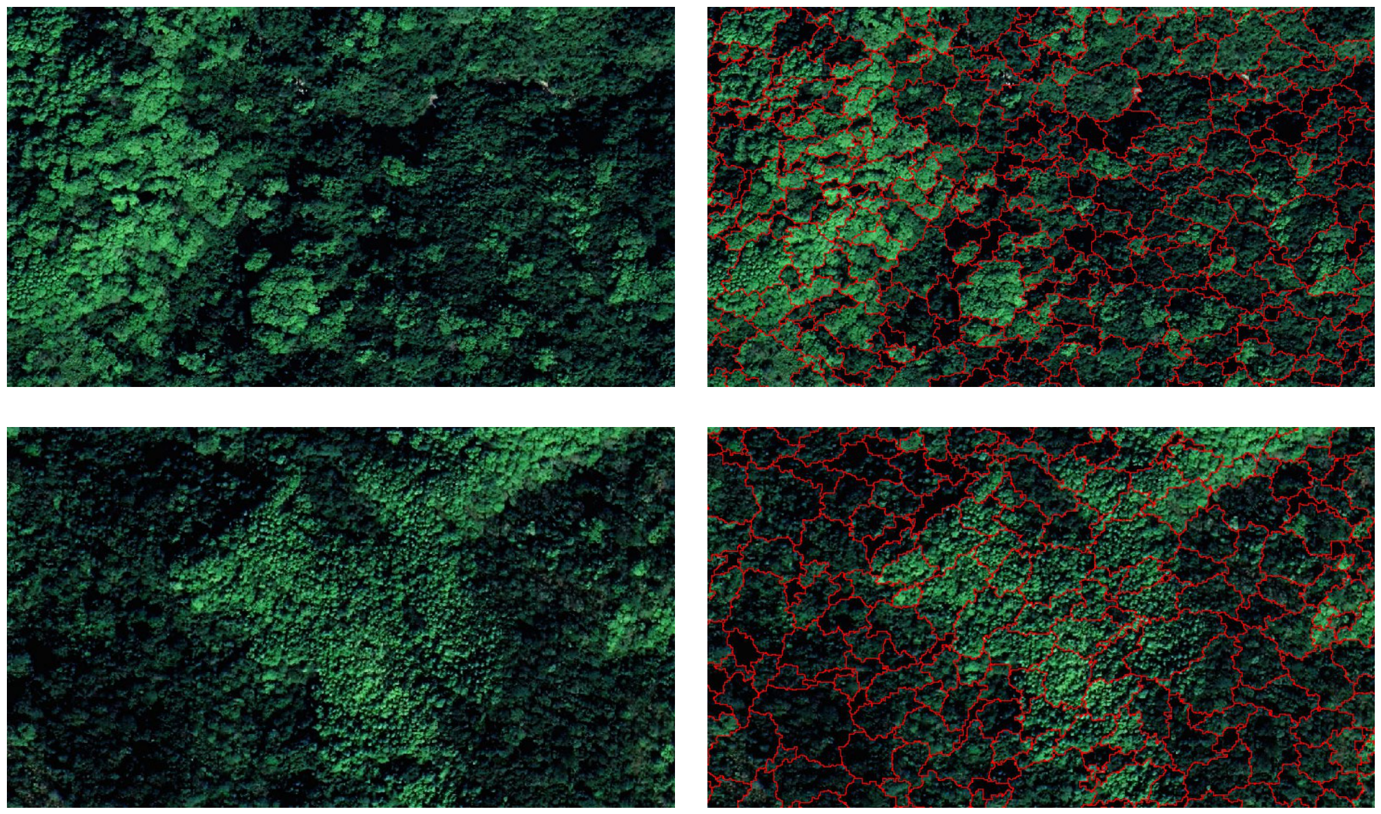
Based on the Google Earth high-resolution imagery, we used the multi-scale segmentation algorithm on the eCognition Developer platform to extract forest stand objects. This algorithm combines adjacent pixels with similar spectral and shape characteristics to create homogeneous forest stand objects. These objects are the basic units for later classification and analysis. Its core principle is to reduce internal object heterogeneity as much as possible, getting optimal segmentation results through iterative optimization. After many rounds of experiments and visual verification, we determined the final optimal segmentation parameters: scale parameter 50, shape weight 0.6, and compactness 0.7. As shown in Figure 2, this parameter combination effectively identifies the natural boundaries of forest stand patches while maintaining spectral and textural homogeneity within objects. It successfully tells different forest stand types apart without obvious over-segmentation or under-segmentation. Based on this, the study finally created forest mapping units that match the spatial pattern of the study area’s forests and have clear ecological significance.
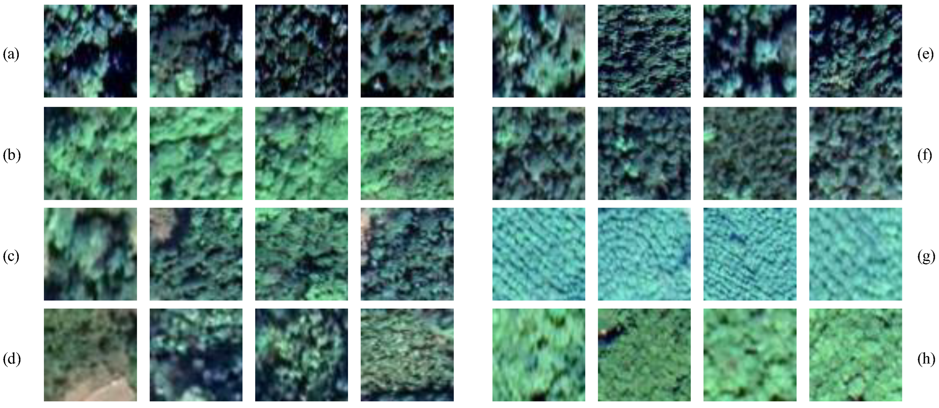
Using tree species data from 41 field survey plots, and combining it with the Flora of Hainan and regional vegetation type maps, we established interpretation guidelines for different forest stand types based on canopy texture features visible in Google Earth imagery. We assigned accurate category labels to each segmented forest stand object, resulting in a total of 1628 labeled objects. Samples of different stand types are shown in Figure 3.
Using the minimum bounding rectangle of each forest stand object as the boundary, we cropped corresponding image patches from the aligned multi-source imagery to use as training samples. By statistically analyzing the bounding rectangle sizes of all objects in the study area, we uniformly standardized the input sample size for the model to 128 × 128 pixels to reduce interference from non-target background information.
Data augmentation is an effective strategy to enrich training sample diversity. In this study, we apply conventional geometric transformations, including 90°, 180°, and 270° rotations as well as horizontal and vertical flips. These operations are performed directly on real remote sensing images, so the generated samples retain the original spectral information, spatial texture, and structural characteristics of actual forest stand scenes. Such methods do not destroy the real data distribution and have low distortion risk, thus ensuring stable performance in practical applications. Considering relatively sufficient labeled samples and complex heterogeneous characteristics of tropical rainforest images used in this study, classical geometric augmentation achieves a good balance between data authenticity and sample diversity.
As shown in Table 2, the original training set had 1120 samples. After augmentation, the total number of training samples reached 6720, with 508 test samples. Finally, we built a classification dataset containing 7228 samples.

2.3. Dual-Branch Feature Fusion Network (DB-FFN)

2.3.1. Overview of the Proposed Model

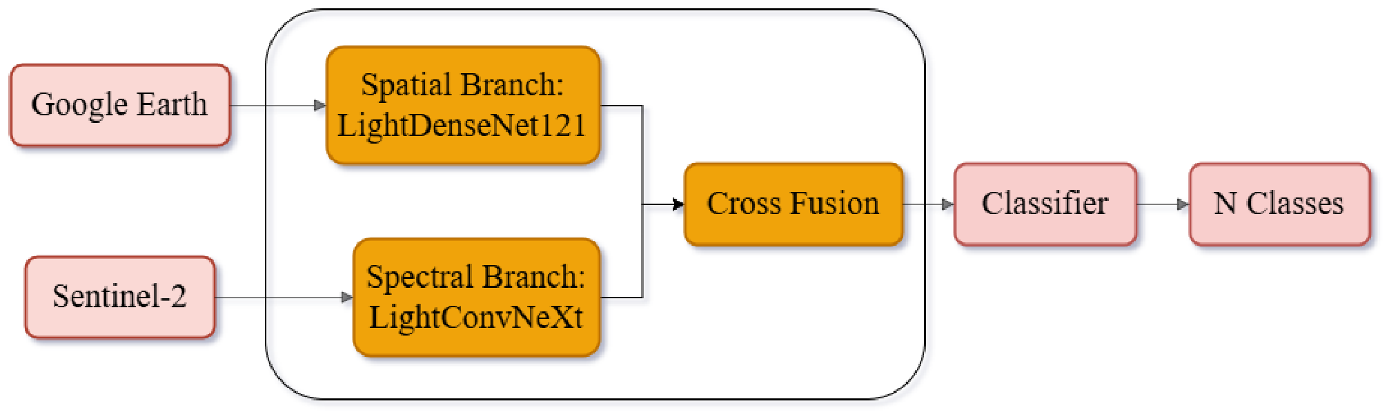
The dual-branch feature fusion network (DB-FFN) we proposed in this study is designed to solve the challenges of fine-grained tree species classification in complex tropical rainforest environments. The overall network architecture is illustrated in Figure 4. Its design mainly includes the following three core features:
First, the model uses a multi-source data collaborative processing mechanism. DB-FFN adopts a parallel dual-branch structure to extract specific features for two types of data: high-resolution spatial texture and multi-temporal spectral sequences. Specifically, the spatial branch is based on an improved DenseNet-121 network. It focuses on capturing the texture and morphological structures of different forest stands from Google Earth imagery. The spectral branch is based on an optimized ConvNeXt-Tiny network. It is dedicated to learning the phenological variation patterns of tree species from Sentinel-2 multi-temporal sequences. Second, the model adds a lightweight attention enhancement design. While ensuring feature extraction capability, the network adds efficient lightweight modules, such as Efficient Channel Attention (ECA) [57], at key positions. These modules adaptively adjust feature responses across channel dimensions with little computational cost, allowing the model to focus on more discriminative information. This effectively improves the model’s robustness and feature utilization efficiency in complex backgrounds.
Finally, the model includes an adaptive gated fusion mechanism. Unlike simple feature concatenation or weighted summation, DB-FFN uses a gated attention unit to dynamically learn and fuse the deep features extracted by the two branches. This mechanism automatically adjusts the contribution weights of spatial texture features and spectral–temporal features in the final decision based on the local context of the input sample. This achieves deeper and more discriminative feature complementarity and synergy, which basically improves the model’s ability to comprehensively use multi-source information.

2.3.2. Time-Series Spectral Feature Extraction Branch

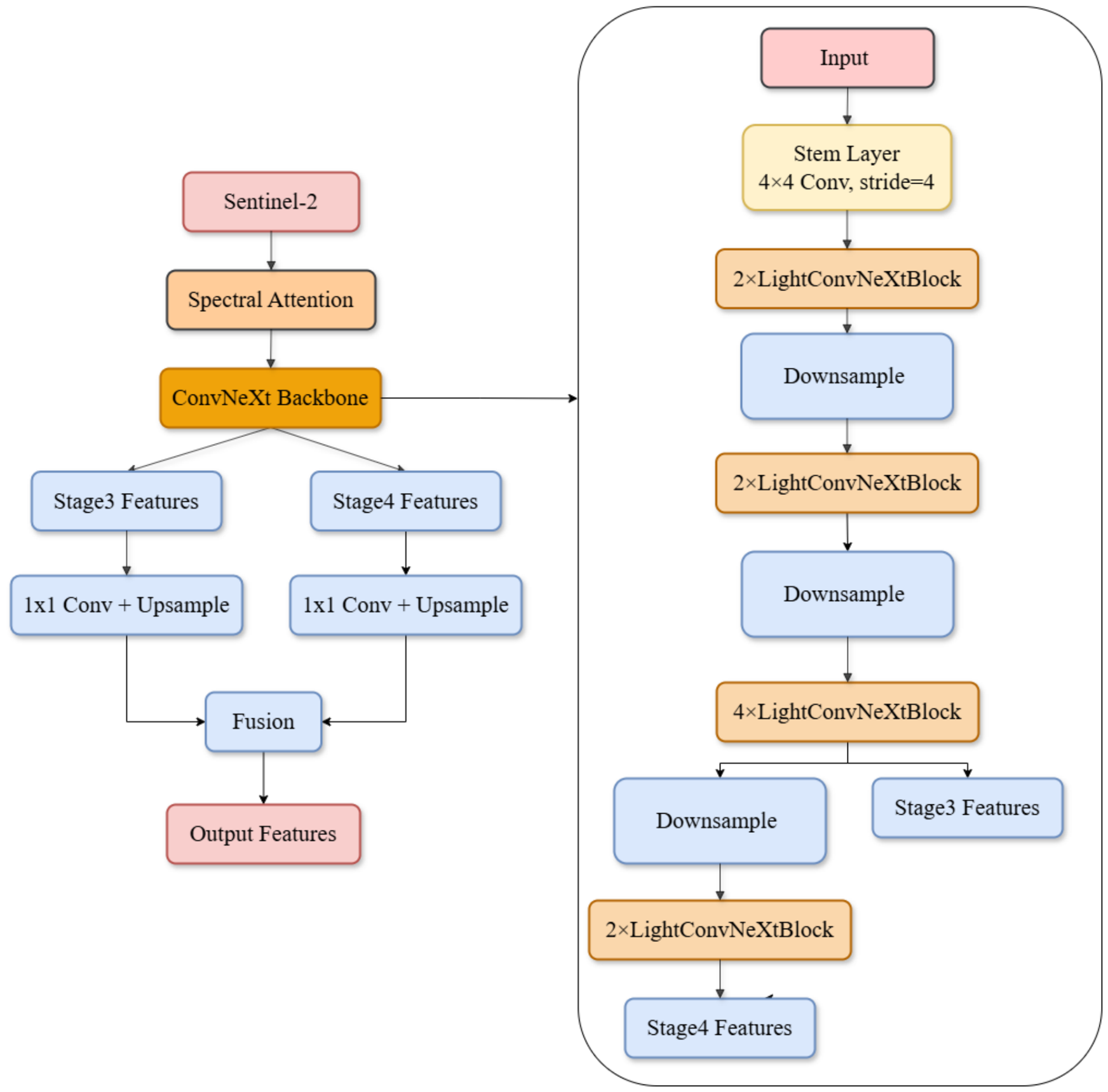
The temporal spectral feature extraction branch uses an improved lightweight ConvNeXt-Tiny structure to extract temporal spectral characteristics from multi-temporal imagery, as depicted in Figure 5. The design of this branch includes three core components: spectral attention preprocessing, hierarchical feature extraction, and multi-scale feature fusion. At the data input stage, the branch first uses a spectral attention module to reweight the original multi-spectral channels. This module uses global average pooling and a two-layer fully connected network to calculate weight coefficients for each channel, aiming to suppress spectral redundancy in multi-temporal data. The feature extraction process has four stages, with the core computational unit being the improved LightConvNeXtBlock. This module first uses a 7 × 7 depthwise separable convolution to expand the receptive field, simulating the long-range dependency capture capability of biological visual systems. This process is expressed as:
X dw   =   DWConv 7 × 7   X in
Then, we perform layer normalization (Layer Norm) on the features and feed them into a feedforward network made up of two layers of pointwise convolution for nonlinear transformation. The computational logic is as follows:
X out   =   W 2   ×   σ   W 1 × X norm
where σ represents the GELU activation function. Before the residual connection, we added a channel attention (ECA) unit to the module. This unit further improves the feature distinguishing capability through adaptive calibration. Finally, we ensure training stability for the deep network through layer scaling and stochastic depth connections. To strengthen the model’s ability to capture features at different scales, the branch builds a multi-scale feature fusion mechanism. The model extracts deep feature maps from Stage 3 and Stage 4, uses 1 × 1 convolutions to uniformly map the channel dimensions to 128, and achieves spatial scale alignment through bilinear interpolation. Finally, the fused features go through batch normalization processing, providing highly distinguishing temporal spectral representations for later multi-source feature collaboration.

2.3.3. High-Resolution Image Feature Extraction Branch

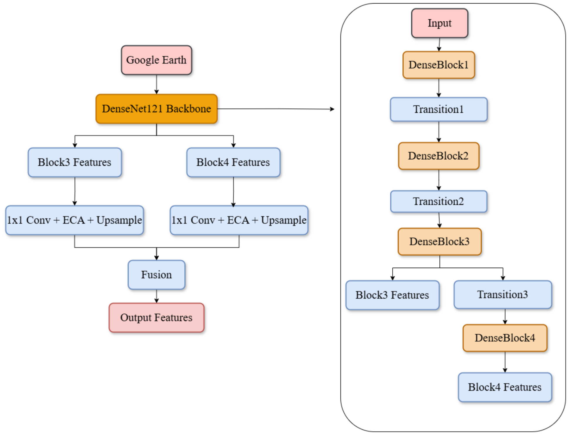
The high-resolution image feature extraction branch adopts DenseNet-121 as the backbone, as depicted in Figure 6. Given the complex textural characteristics of high-resolution remote sensing images, we modified the original network and only utilized output features from DenseBlock 3 and DenseBlock 4. To address the discrepancies in dimension and spatial resolution across multi-level features, a multi-scale feature fusion module is integrated into the model. Specifically, 1 × 1 convolutions are applied to unify all extracted features into 128 dimensions, and bilinear interpolation is adopted for spatial alignment. The mathematical formulation of this fusion process is presented below:
F spatial   =   σ BN i = 3 4 Upsample ECAttention Conv 1 × 1 D i x
where D i represents the feature extraction function of the i-th DenseBlock, BN denotes batch normalization, and σ is the activation function.
In addition, to improve feature distinguishing weighting and control the model scale, we added a channel attention (ECA) module in the feature fusion path. This module adaptively learns inter-channel interaction information through one-dimensional convolution. It effectively focuses on high-value texture information and suppresses background noise without greatly increasing the parameter burden. The calculation process of its attention weights is as follows:
ω   =   Sigmoid Conv 1 D k GAP F
where GAP denotes Global Average Pooling, and Conv 1 D k represents 1D convolution with a kernel size of k. Through the aforementioned structural optimization and attention enhancement, this branch achieves precise extraction of morphological and structural features of ground objects.

2.3.4. Feature Fusion and Classification

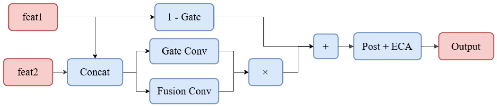
In this work, spatial texture and spectral–temporal features represent forest stand information in quite different ways. To deal with this mismatch, we designed a gated attention fusion mechanism. It adjusts the contribution from each data source, as depicted in Figure 7.
The feature fusion mechanism was put at the end of the two independent feature extraction branches. This choice avoids the problems of early fusion. Early fusion combines the raw input data directly. When spatial and spectral information are mixed at the very beginning, their feature distributions and value scales often do not match well. This mismatch disrupts the early convolution layers. The network then finds it hard to capture fine canopy texture and long-term phenological changes separately.
The proposed model takes a different path. It uses two dedicated backbones to learn unique semantic features from spatial texture and from spectral–temporal data. Each branch works independently. It screens features, abstracts high-level information, and suppresses noise based on its own data type. We wait until both branches have produced high-dimensional, representative features. Only then do we fuse them. At this point, the gated unit can judge how useful each feature type is for a given forest stand sample. This provides a reliable base for adaptively redistributing the weights.
In our processing pipeline, the two branches first produce separate feature streams. Once extracted, these streams are connected. A gating unit then creates mask weights. The goal is to let the mechanism adaptively change how much the spatial branch and the spectral branch each contribute. This decision is based on how informative a pixel is for telling different forest stand types apart. As a result, the model can suppress redundant or noisy information that comes from a single source. We can formally express the fusion as:
F fused   =   G   ×   Φ   F spatial , F spectral   +   1     G ×   F spatial
Here, Fspatial and Fspectral represent the output features of the spatial branch and the spectral branch, respectively. denotes the channel concatenation operation, Φ is the fusion transformation function, and G ∈ {0, 1} is the adaptive gate weight learned by the model through the gated convolutional layer. This structure allows the model to dynamically add distinguishing spectral phenological information while retaining the high-resolution spatial structures, based on the characteristics of input samples. After feature fusion, the classification module uses Global Average Pooling (GAP) to compress the spatial dimension into a feature vector. Then we map this vector through a classifier made up of two layers of Multi-Layer Perceptrons (MLP). To improve the model’s generalization capability and training stability, we add Dropout random deactivation and BatchNorm batch normalization layers in the classifier. The final output layer uses the Softmax function to calculate the predicted probability distribution across N categories:
P i   =   e z i j = 1 N e z j
in which, Pi denotes the probability that the sample belongs to the i-th forest classification category, and z represents the raw output value of the classification head.
After feature interaction is finished, the classifier is responsible for mapping the fused high-level semantic features into the class label space. This structure uses Global Average Pooling and a two-layer Multilayer Perceptron (MLP) in sequence. The former compresses feature redundancy and retains global contextual information by downsampling the spatial dimensions, while the latter achieves distinguishing transformation and dimensionality reduction of tree species features through nonlinear transformations. The final output layer is normalized by the Softmax function to get the predicted probability for each class:
P y   =   i | x   =   exp   w i T F fused   +   b i j = 1 N exp   w j T F fused   +   b j
in which, i = 1, 2, …, N represents the N tree species categories.

2.4. Controlled Experiments

2.4.1. Experimental Setup

To evaluate the contribution of multi-temporal and multi-source data to tropical rainforest tree species classification and validate the performance of the dual-branch feature fusion network (DB-FFN) we proposed in this paper, we designed the following controlled experiments.
For model selection, five widely used convolutional neural networks—VGG-16, ResNet-18, GoogLeNet, DenseNet-121, DBAF-Net [54] and ConvNeXt—were selected as comparative models. In terms of data configuration, four experimental data setups were adopted. The first setup used single-date Sentinel-2 data (containing only November imagery) as the baseline to assess the fundamental spectral classification capability. The second setup employed multi-temporal Sentinel-2 data (including January, March, August, and November imagery) to examine the accuracy improvement achieved by adding phenological temporal features. The third setup utilized high-resolution Google Earth imagery to evaluate the role of spatial texture features. The fourth setup adopted the fused data combining Google Earth and multi-temporal Sentinel-2 to explore the potential of multi-source information synergy.
We trained and tested all comparative models under the four data setups mentioned above. By comparing their performance metrics, we can analyze the influence of spatial texture features and temporal phenological features on classification accuracy. The DB-FFN network we built in this study is specifically designed to integrate two types of data: high-resolution spatial texture and multi-temporal spectral sequences. So, we only trained and evaluated this model under the fourth data setup (that is, multi-source fused data). By comparing the performance of DB-FFN under this data condition with the performance of each baseline model under the same condition, we can validate the effectiveness of the proposed dual-branch fusion mechanism in synergizing multi-source features.

2.4.2. Model Training Parameters

The experiments were conducted using the PyTorch framework and executed on an NVIDIA RTX 3080 GPU. Model training utilized the Adam optimizer with an initial learning rate of 0.0001, a batch size of 8, and a maximum training epoch limit of 70. Model parameters were initialized using the He normal distribution method.
To mitigate overfitting and control model complexity, multiple regularization strategies were employed: a weight decay coefficient of 1 × 10⁻⁴ was set, a dropout rate of 0.2 was introduced in the fully connected layers, and the cross-entropy loss function was selected for model optimization. In terms of training scheduling, a dynamic adjustment mechanism was implemented: if the improvement in overall validation accuracy fell below 1 × 10⁻⁴ over 8 epochs, the learning rate was reduced to 0.1 times its previous value. Additionally, an early stopping mechanism was introduced, where training was automatically terminated if the validation loss did not decrease for 20 epochs, ensuring the model’s generalization performance.

2.4.3. Evaluation Indicators

To evaluate the performance of the classification model, we use a series of statistical metrics based on the confusion matrix. These specifically include Overall Accuracy (OA), Kappa coefficient, User’s Accuracy (UA, corresponding to precision), Producer’s Accuracy (PA, corresponding to recall), and F1-score (F1). These metrics give a comprehensive evaluation of the model’s classification results from different angles: OA shows overall classification accuracy, the Kappa coefficient measures the consistency difference between classification results and random classification, UA shows the reliability of predictions for each category (that is, the proportion of samples predicted as a certain class that are actually that class), PA shows the completeness of recognition for each category (that is, the proportion of samples that are actually a certain class and are correctly predicted), while the F1 score balances precision and recall to fully reflect the model’s classification robustness.
Overall Accuracy shows the model’s classification correctness across the entire dataset, defined as the proportion of correctly classified samples relative to the total number of samples:
OA   =   i = 1 C TP i N
We use the Kappa coefficient to measure the consistency between classification results and random classification, and it effectively removes the influence of chance correct classifications. We calculate it based on observed accuracy and expected accuracy:
κ   =   OA     P e 1   P e
where P e   =   i = 1 C TP i   +   FN i   ×   TP i   +   FP i N 2 is the expected precision.
User Accuracy (UA), corresponding to Precision in statistics, shows the reliability of classification results. It represents the proportion of samples labeled as class i on the classification map that actually belong to that class in the ground truth. A higher value means the model has lower commission error. Its formula is:
UA i   =   T P i T P i   +   F P i
Producer Accuracy (PA), corresponding to Recall, shows a model’s ability to identify specific feature categories or its completeness rate. It represents the proportion of samples with actual ground truth of class i that are correctly classified as that class by the model. This metric reflects the degree of omission error; a higher PA value means the model has fewer misclassifications of that tree species. Its calculation formula is:
PA i   =   T P i T P i   +   F N i
In addition, to fully balance user precision and producer precision and avoid evaluation biases caused by relying on a single metric, we use the F1 score as a harmonic mean of the two. The F1 score gives a more robust assessment of a model’s overall performance across tree species categories. Its calculation formula is:
F 1 i   =   2   ×   UA i   ×   PA i UA i   +   PA i
Among these, TPi (True Positives) denotes the number of samples correctly classified as class i, FPi (False Positives) represents the number of samples from other classes mistakenly classified as class i, and FNi (False Negatives) indicates the number of class i samples incorrectly classified as other classes. Through this metric system, the model’s classification performance in complex rainforest environments can be comprehensively validated across three dimensions: overall accuracy, prediction reliability (UA), and identification sensitivity (PA).

3. Results

(1)
The Comparative Experiment
Table 3, Table 4, Table 5 and Table 6 report the classification results of DB-FFN and the six benchmark models (VGG-16, ResNet-18, GoogLeNet, DenseNet-121, ConvNeXt, DBAF-Net [54]) under four data setting. This section analyzes the results based on five aspects. The first aspect compares single-date and multi-temporal Sentinel-2 data and assesses the contribution of phenological information. The second aspect evaluates the effect of combining high-resolution Google Earth imagery with multi-temporal Sentinel-2 data. The third aspect compares DB-FFN with the benchmark models under the fused data setting. Class-level accuracy and the final spatial classification map are also reported. The fourth aspect analyzes the accuracy of different tree species categories under the DB-FFN model to clarify the recognition accuracy of each tree species category. The fifth aspect presents the forest stand tree species classification map of the study area under the DB-FFN model to analyze the distribution of each forest stand type in the study area.
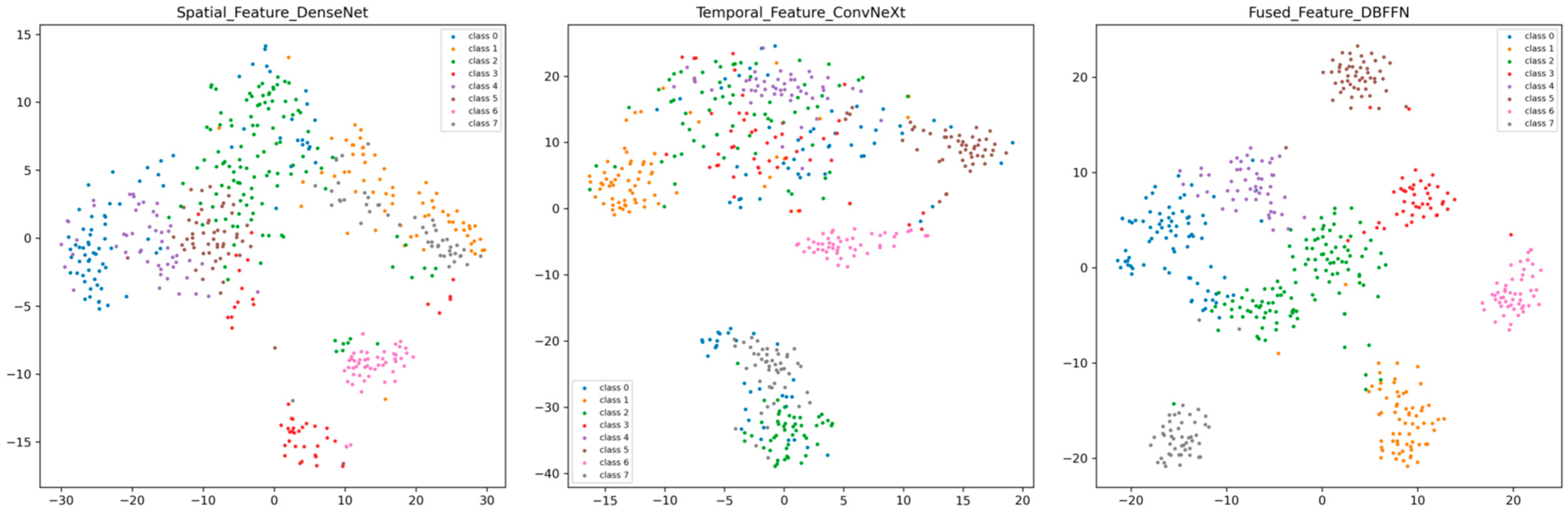
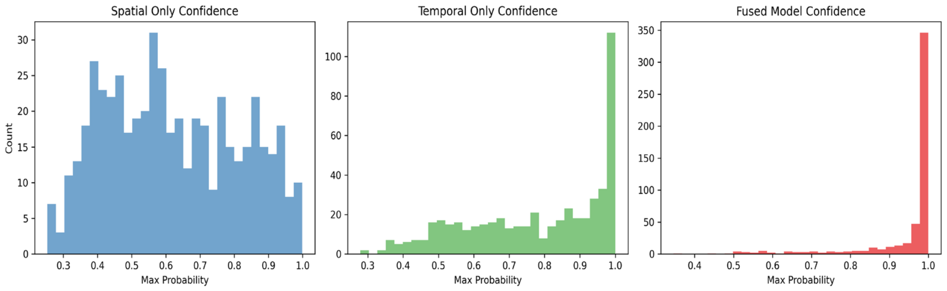
To understand what each branch had learned, we used t-SNE to reduce the feature dimensions and visualize their distribution as shown in Figure 8 and Figure 9. The spatial branch captured fine canopy texture and structural information. The temporal branch focused on seasonal spectral variation and phenological characteristics. When we looked at the plot, the two feature sets showed clearly different distributions. This separation suggests strong complementarity between the two types of features. We also looked at the posterior probability distributions from three prediction modes: spatial-only, spectral–temporal-only, and the fused dual-branch model. The single-modal outputs showed scattered confidence values. Many samples fell in the uncertain middle range. After fusion, the confidence values clustered at the high end. This shift tells us that fusing both modalities reduces uncertainty. The classification becomes more stable and reliable.
The computational complexity of DB-FFN primarily comes from two parts that perform feature extraction. One part is the spatial branch built on DenseNet121, and the other is the temporal branch built on ConvNeXt-Tiny. These two branches together take up most of the network’s computation cost. They carry out nearly all of the feature extraction and transformation work. In contrast, the gated fusion module only performs light feature interaction and adaptive weight adjustment. This module adds almost no computation. Thus, when the input spatial size grows, the model’s total computational complexity rises steadily.
For a more precise measure of the actual computation cost and running efficiency, three common indicators are used. These are FLOPs, Params, and inference time. FLOPs mean the total floating-point operations in the network. This number directly shows how much calculation is done. Params are the total number of trainable parameters. They reflect the model’s size, how much memory it needs, and the chance of overfitting. Inference time is the average time spent on processing one test sample. It directly tells us how fast the model makes predictions and how well it can be deployed in practice. Taken together, these three measures give a full and clear picture of the model’s computation cost and operating efficiency.
Looking at the number of parameters as shown in Table 7, the DB-FFN model has 12.74 million parameters. This number is much smaller than that of VGG16 or ConvNeXt-Tiny. At the same time, it stays at a similar scale as ResNet18 and GoogLeNet. This shows that the better performance of the proposed model does not come from simply making the model bigger.
For computational complexity, DB-FFN has 1.56 GFLOPs. This value is lower than those of VGG16, ResNet18, DenseNet121, and GoogLeNet, and is only a bit higher than that of ConvNeXt-Tiny. For inference speed, ResNet18 has the lowest delay because its structure is simple. DB-FFN uses two branches for feature extraction and fusion. Because of this design, it takes a little more inference time than single-branch networks. Still, its inference efficiency is better than that of DenseNet121.
Taking everything together, the proposed DB-FFN gives better classification accuracy while keeping a moderate number of parameters, low computational complexity, and acceptable inference speed. This shows a good balance between classification performance and computational cost.
(2)
The Multi-round Repeated Experiment
To remove the randomness caused by model initialization and data loading order, five independent runs with different random seeds were carried out for each of the compared models. All experiments shared hyperparameter settings, and hardware environment. Table 8 reports the mean, standard deviation, maximum, and minimum values of overall accuracy (OA) and Kappa coefficient.
As shown in Table 8, DB-FFN achieved the highest average OA (0.9315) and Kappa (0.9202) among all methods. It also obtained the best maximum values: an OA of 0.9449 and a Kappa of 0.9360. Although its standard deviation was slightly larger than that of some baseline models, its lowest OA and Kappa values were still higher than those of most other networks. The classic backbone networks exhibited relatively small standard deviations. This indicates stable performance across different runs. DenseNet121 and ConvNeXt achieved similar average accuracies, and both offered competitive classification capability. ResNet18 recorded the lowest average accuracy. VGG16 and GoogLeNet fell in the middle with moderate overall performance. Overall, the dual-branch fusion structure effectively extracts complementary spatial and spectral features. This design leads to a steady improvement in performance compared with single-branch mainstream models.
(3)
The Ablation Experiment
Ablation experiments as shown in Table 9 were conducted to quantify the contribution of each core module. The baseline dual-branch model, without the attention mechanism and gated fusion, obtained an overall accuracy of 92.41% and a Kappa of 0.91. The complete DB-FFN model reached an overall accuracy of 94.49% and a Kappa of 0.94, an increase of 2.08 percentage points. This result demonstrates the clear benefit of integrating all components.
Removing the ECA attention mechanism caused the accuracy to drop to 92.91% and the Kappa to 0.92. The numerical gap suggests that the attention module helps enhance effective feature weights and brings a tangible gain in performance.
When only a single branch was used, the classification ability dropped sharply. The RGB branch achieved an overall accuracy of 88.78% and a Kappa of 0.87, while the multispectral branch obtained only an overall accuracy of 82.68% and a Kappa of 0.80. The large difference between single-branch and dual-branch results indicates that neither modality alone can support high-accuracy classification. The two branches supply irreplaceable complementary information.
Removing the gated fusion module reduced the accuracy to 93.31% and the Kappa to 0.92, a drop of 1.18 percentage points compared with the full model. This confirms that the adaptive gated fusion mechanism can properly allocate feature weights and effectively improve classification performance. Overall, all components work together to achieve the best comprehensive result.

3.1. Effect of Multi-Temporal Information on Classification Accuracy

A comparison between Table 3 and Table 4 shows that all five benchmark models performed better with multi-temporal Sentinel-2 data than with single-data Sentinel-2 data. The overall accuracy (OA) of ConvNeXt increased from 62.40% to 83.07%, which corresponds to a gain of 20.67 percentage points. The OA of ResNet-18 increased from 58.86% to 80.12%, a gain of 21.26 percentage points. GoogLeNet increased from 61.81% to 83.27%, an increase of 21.46 percentage points. DenseNet-121 increased from 60.04% to 82.09%, a gain of 22.05 percentage points. VGG-16 increased from 58.86% to 74.02%, a gain of 15.16 percentage points. Among the five models DenseNet-121 showed the largest improvement, whereas VGG-16 showed the smallest gain.
The Kappa coefficient showed the same pattern. It increased from 0.52–0.56 in the single-date setting to 0.70–0.81 in the multi-temporal setting. These results suggest that the images acquired in January, March, August, and November provided useful phenological information for tree species discrimination. Relative to single-date imagery, the multi-temporal setting appears to reduce classification confusion caused by similar spectral responses among different classes. This pattern was observed across all tested models.

3.2. Effect of Multi-Source Data Fusion on Classification Accuracy

A comparison of Table 4, Table 5 and Table 6 shows a consistent ranking across data setting. For all methods, the fused setting—that is, Google Earth imagery combined with multi-temporal Sentinel-2 data—produced the highest accuracy. The Google Earth-only setting ranked second, the multi-temporal Sentinel-2-only setting ranked third, and the single-date Sentinel-2 setting ranked last.
Relative to single-date Sentinel-2 baseline, the fused data setting improved OA by 30.91 percentage points for ConvNeXt, 34.05 percentage points for ResNet-18, 30.32 percentage points for GoogLeNet, 32.28 percentage points for DenseNet-121, and 32.28 percentage points for VGG-16. The Kappa coefficients followed the same trend and reached 0.90–0.92 in the fused setting, which was higher than the corresponding values in the single-source settings.
The gain from the multi-temporal Sentinel-2 setting to the fused setting was also clear. OA increased 10.24 percentage points for ConvNeXt, 12.79 percentage points for ResNet-18, 8.86 percentage points for GoogLeNet, 10.23 percentage points for DenseNet-121, and 17.12 percentage points for VGG-16. These results indicate that high-resolution spatial information and multi-temporal spectral information are complementary in this dataset. Google Earth imagery contributed fine canopy texture and spatial pattern, whereas multi-temporal Sentinel-2 data contributed seasonal spectral variation. Their joint use improved classification performance in complex tropical forest scenes.

3.3. Performance of DB-FFN Under the Fused Data Setting

Under the fused setting of Google Earth imagery and multi-temporal Sentinel-2 data, DB-FFN achieved the best overall performance among all evaluated models. Its OA reached 94.49%, and its Kappa coefficient reached 0.94. Under the same data setting, DB-FFN outperformed the best benchmark model, ConvNeXt, by 1.18 percentage points in OA. It also exceeded GoogLeNet, ResNet-18, DenseNet-121, and VGG-16by 2.36, 1.58, 2.17, and 3.35 percentage points, respectively.
The advantage of DB-FFN was also evident when it was compared with the best results obtained under each single-source setting. Its OA was 4.92 percentage points higher than the best Google-Earth-only result, which was achieved by DenseNet-121 at 89.57%. It was 11.22 percentage points higher than the best multi-temporal Sentinel-2-only result, which was achieved by GoogLeNet at 83.27%. It was also 32.09 percentage points higher than the best single-date Sentinel-2-only result, which was achieved by ConvNeXt at 62.40%. These results support the use of a dual-branch architecture for the joint use of spatial texture information and temporal spectral information.

3.4. Class-Level Accuracy of the DB-FFN Mode

Table 10 presents the confusion matrix of the DB-FFN model and the producer’s accuracy (PA), user’s accuracy (UA), and F1-Score for each forest stand type. Overall, the class-level results are high, but the performance varied across classes.
Among the plantation classes, Caribbean pine plantation and rubber plantation showed very high classification accuracy, with PA, UA, and F1-Score close to or at 100%. Pinus latteri plantation also showed stable performance, with an F1-Score of 97% and both PA and UA above 96%. Tropical montane rainforest primary forest reached a PA of 95% and a UA of 90%, which suggests limited but non-negligible confusion with other forest types.
Tropical deciduous/semi-deciduous rainforest achieved an F1-Score of 96%, with a UA of 100% and a PA of 92%. This pattern suggests that predictions assigned to this classes were highly reliable, although some reference samples of this classes were still assigned to other categories. Lowland rainforest secondary forest had the lowest F1-Score among the eight classes, at 91%, which indicates that it has remained the most difficult class to separate. It errors involved several other categories, including tropical deciduous/semi-deciduous rainforest and betel nut palm plantations. This result is consistent with the high heterogeneity of secondary forests in species composition, structure, and phenology.
Artificial plantations typically consist of a single tree species and have a uniform stand structure. In contrast, lowland rainforest secondary forest develops through natural succession and community recovery after disturbance. This forest contains a mixture of trees, shrubs, and herbaceous plants, which creates a highly complex species composition. Spatially, the canopy texture is irregular and fragmented. It lacks the regular crown shapes seen in artificial forests. Phenologically, the mixed tree species do not grow and shed leaves at the same time. This asynchronous rhythm leads to constantly changing seasonal spectral characteristics. The complex spatial texture and asynchronous phenology cause its spectral signature to overlap strongly with those of neighboring forest types. As a result, inter-class confusion is most severe and classification accuracy is the lowest.
Betel nut palm plantation also showed high class-level accuracy, with a UA of 98% and a PA of 96%, which indicates only limited confusion. Lowland rainforest showed a high PA of 98% but a lower UA of 88%. This pattern suggests that most reference samples of this class were identified correctly, but some reference samples were also predicted as other categories, such as tropical montane rainforest primary forest and Pinus latteri plantations. Overall, the remaining confusion appears to be associated with similarities in canopy structure, seasonal behavior, and community-level spectral response among different forest stand types.

3.5. Forest Stand Classification Map Produced by DB-FFN

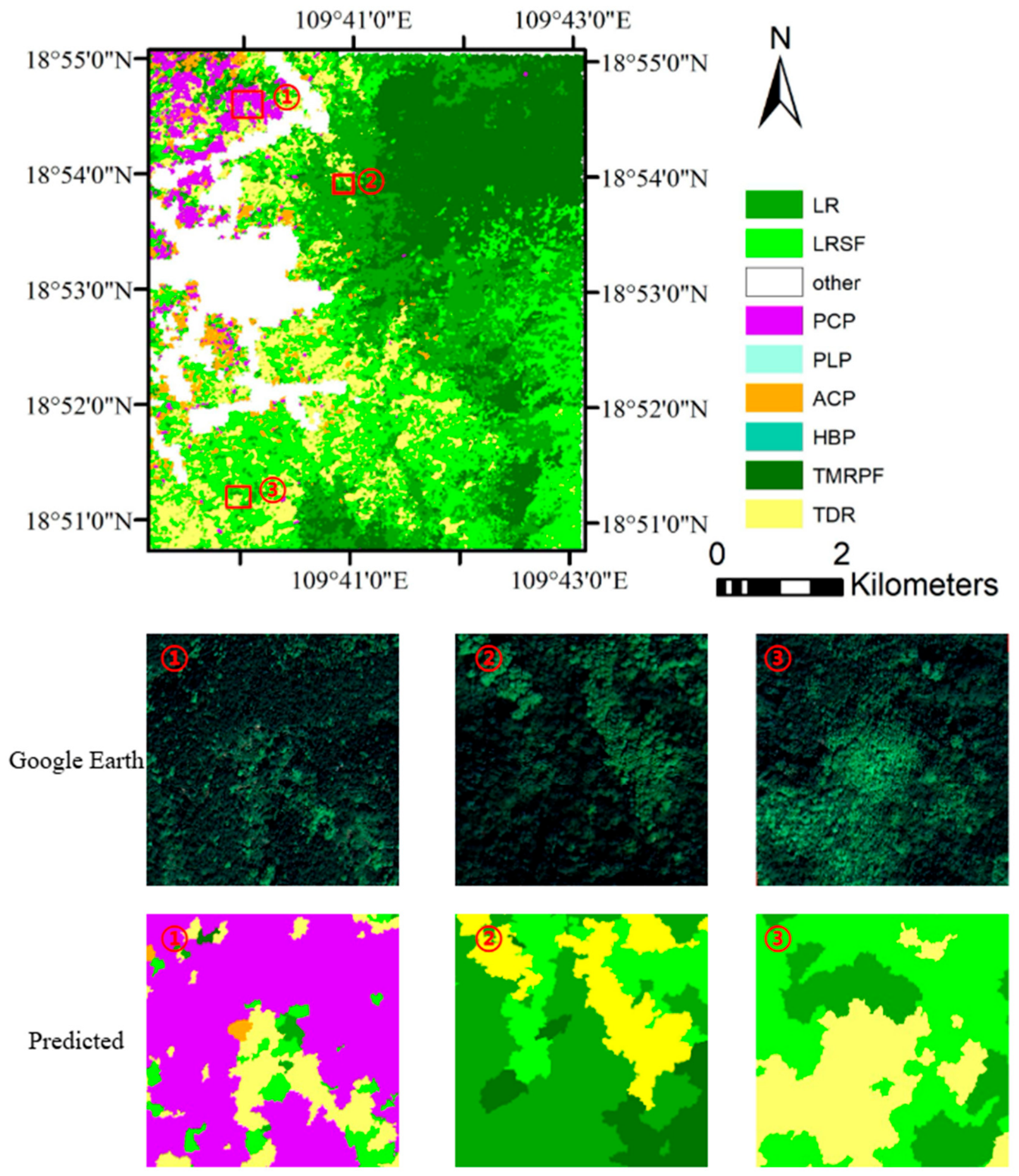
Figure 10 shows the forest stand classification map produced by DB-FFN. The map captures clear spatial heterogeneity and a mosaic distribution pattern across the study area.
Natural forest stands, including tropical montane rainforest primary forests and lowland rainforests, were concentrated mainly in topographically complex areas. Their patches exhibit irregular shapes and their boundaries were relatively complex. By contrast, managed plantation types, including Caribbean pine, rubber, and betel palm, showed more regular and concentrated patches. These patches are often located near roads or cultivation areas.
Lowland rainforest secondary forest and tropical deciduous/semi-deciduous rainforest were more scattered and were often interwoven spatially. This pattern may reflect differences in recovery stage and disturbance history. Overall, the map captured the main distribution patterns and patch boundaries of the major forest stand types. These findings suggest that the multi-source data fusion approach can support forest stand classification and spatial mapping in complex tropical environments. The resulting map can provide a spatial basis for subsequent analyses of biodiversity, forest succession, and ecosystem management.

4. Discussion

4.1. Role of Multi-Temporal and Multi-Source Data Fusion

This study indicates that multi-temporal phenological information made an important contribution to tropical rainforest tree species classification in this classification task. In single-date imagery, many tree species were difficult to distinguish because canopy spectral responses overlapped strongly. By using imagery from four time points, January, March, August, and November, the model was able to capture the seasonal spectral variation among species. This variation is related to changes in leaf pigments, water content, and phenological stage. It therefore provided additional information for separating classes with similar spectral responses. For example, the OA of ConvNeXt increased from 62.40% with single-date Sentinel-2 data to 83.07% with multi-temporal Sentinel-2 data, which represents a gain of 20.67 percentage points. In this dataset, temporal phenological information provided more discriminative information than single-data spectral features alone. It also reduced confusion associated with the problem of “different objects with similar spectra.”
A major cause of this confusion lies in the limited spectral information offered by high-resolution RGB imagery. Such data simply cannot capture enough spectral detail for accurate forest stand classification. Many distinct tree species look very similar in RGB images. Their colors and visual textures overlap heavily, which leads to serious spectral mixing and greater classification uncertainty. These inherent drawbacks restrict both the accuracy and the reliability of using RGB data alone. To address this problem, multisource remote sensing data and effective fusion strategies are needed. They can compensate for the weaknesses of each single data type.
High-resolution imagery, such as Google Earth imagery, captured canopy texture, crown form, and spatial patterns in fine detail, but it did not provide seasonal spectral variation. Multi-temporal spectral data recorded phenological change, but they contained less spatial detail. When these two resources were combined, they provided a more complete description of forest stands. This pattern can be seen in the DenseNet121 results. Under the fused setting, DenseNet121 reached an OA of 92.32%. Under the Google Earth-only setting, its OA was 89.57%. Under the multi-temporal Sentinel-2-only setting, its OA was 82.09%. These results suggest that the two data sources provided complementary information and helped reduce the limitations of single-source classification in complex forest scenes.

4.2. Role of Branch-Specific Feature Extraction and Adaptive Fusion in DB-FFN

DB-FFN differed from the benchmark models in the way that multi-source inputs were handled. Under the fused data setting, the benchmark models received the two data sources through direct concatenation of Google Earth imagery and multi-temporal Sentinel-2 data. By contrast, DB-FFN processed the two data sources through two dedicated branches before feature fusion.
The performance of DB-FFN may be related to two parts of its design: branch-specific feature extraction and adaptive fusion. The DenseNet branch is used to extract spatial textural features from high-resolution imagery. These features may help represent canopy boundary, local pattern, and crown shape. The ConvNeXt branch is used to model temporal dependence in the multi-temporal spectral sequence. This branch may help represent seasonal variation among forest stand types. The gated attention module then combines the two feature streams. This design allows the model to place different emphasis on spatial and temporal information for different samples.
The experimental results suggest that this design was effective for the present task. Under the fused data setting, DB-FFN achieved an OA of 94.49%, which was 1.18 percentage points higher than the best benchmark model, ConvNeXt. Because the comparison models under the same setting used direct concatenation of the two data sources, this result suggests that simple concatenation was less effective than branch-specific feature extraction followed by adaptive fusion in this dataset. The result also indicates that, in complex tropical rainforest environments, heterogeneous data sources may be used more effectively when each source is modeled through a dedicated pathway before integration.

4.3. Limitations

The dataset used in this study has small problems with sample size and class distribution. These problems are common in remote sensing work on tropical forests. Collecting field samples in the Hainan tropical rainforest is difficult because of the complex terrain, dense plants, and limited access. This makes it hard to get enough labeled samples that are evenly spread across different classes. On top of that, different tree species naturally occur in different numbers. These sampling difficulties, together with natural differences in species abundance, cause small differences in the number of samples across forest stand classes. For classes that have a relatively sufficient number of samples, the model can learn stable feature representations. For classes with fewer samples, the model may not capture all the important features. This could have small negative effects on classification performance.
To make the training data more diverse, this study uses simple geometric augmentation methods. These include rotation and flipping. They are used to expand the training dataset. These simple transformations can increase sample variety. However, they only rearrange the pixel information that is already there. They do not create new spectral or spatial features. Because of this, such augmentation methods cannot add new useful feature information. They can only reduce the small differences in sample quantity and distribution across tropical forest classes, not completely fix them.
There are two main ways to expand training samples: data augmentation and data generation. Simple geometric augmentation has only a limited effect on improving the sample problem. Because of this, later studies can try using generative data generation methods. One example is the vMRF-based GANSO method [58]. This method can improve sample quality and make the class distribution more balanced. Unlike geometric augmentation, which only changes the arrangement of pixels, the vMRF-constrained GANSO method can retain the spatial connections and structural features of the original remote sensing images when it creates new samples. This matches the real-scene properties that the augmentation method used in this study also tries to maintain. This type of generative method works well for datasets with a small class imbalance. It can also handle cases where there are not enough labeled samples. It provides a possible way to improve the generalization performance of tropical forest stand classification models in future work.

5. Conclusions

This study examined fine-grained tree species classification in tropical rainforests by combining high-resolution Google Earth imagery with multi-temporal Sentinel-2 data. Meanwhile, a dual-branch feature fusion network (DB-FFN) was developed to explore the value of independent feature learning and adaptive fusion for different data types. Classic benchmark models were compared under multiple experimental data settings.
Three main findings can be drawn from this study. First, multi-temporal phenological information improves class separability by capturing seasonal spectral variations that single-phase imagery cannot fully reflect. It relieves the problem of similar spectral features among different tree species in complex tropical environments. Second, high-resolution spatial information and multi-temporal spectral information are complementary: the former characterizes canopy texture and spatial structure, while the latter captures long-term phenological dynamics, and their integration achieves a more comprehensive representation of complex forest stand features. Third, the customized fusion design improves classification performance. The multi-source fused data outperforms single data sources, and the proposed DB-FFN achieves the optimal overall effect. This indicates that extracting spatial and spectral–temporal features through separate branches before adaptive fusion is well suited to make full use of heterogeneous remote sensing data.
This study suggests that phenology should be regarded as a core dimension in tropical rainforest tree species classification. It also proves that combining high-resolution texture data and multi-temporal satellite data can support accurate fine-scale mapping in complicated forest areas. From a methodological perspective, separate feature extraction for different data sources, followed by adaptive fusion, can enhance the utilization efficiency of multi-source heterogeneous information.
Future research can validate the generalizability of this framework across more tropical forest regions and diverse temporal scenarios. Additional data such as UAV hyperspectral imagery and LiDAR can be integrated to enrich multi-dimensional feature systems. Moreover, introducing cross-regional transfer learning will further strengthen the model’s practical adaptability in different tropical forest environments.


Author Contributions

Conceptualization, J.H., H.L., L.J. and X.S.; Methodology, J.H., H.L., L.J. and X.S.; Software, J.H. and L.J.; Validation, J.H.; Resources, L.J.; Data curation, J.H.; Writing—original draft, J.H.; Writing—review & editing, J.H.; Visualization, J.H.; Supervision, H.L.; Project administration, H.L. and L.J.; Funding acquisition, H.L. and L.J. All authors have read and agreed to the published version of the manuscript.

Funding

This research was supported by Hainan Provincial Natural Science Foundation of China (424CXTD433).

Data Availability Statement

The data that support the findings of this study are available from the corresponding author upon reasonable request.

Conflicts of Interest

The authors declare no conflicts of interest.

References

  1. Pan, Y.; Birdsey, R.A.; Fang, J.; Houghton, R.; Kauppi, P.E.; Kurz, W.A.; Hayes, D.; Phillips, O.L.; Shvidenko, A.; Lewis, S.L.; et al. A large and persistent carbon sink in the world’s forests. Science 2011, 333, 988–993. [Google Scholar] [CrossRef] [PubMed]
  2. Sala, O.E.; Stuart Chapin, F.I.I.I.; Armesto, J.J.; Berlow, E.; Bloomfield, J.; Dirzo, R.; Wall, D.H.; Huber-Sanwald, E.; Huenneke, L.F.; Jackson, R.B.; et al. Global biodiversity scenarios for the year 2100. Science 2000, 287, 1770–1774. [Google Scholar] [CrossRef] [PubMed]
  3. Lewis, S.L.; Edwards, D.P.; Galbraith, D. Increasing human dominance of tropical forests. Science 2015, 349, 827–832. [Google Scholar] [CrossRef] [PubMed]
  4. Myers, N.; Mittermeier, R.A.; Mittermeier, C.G.; Da Fonseca, G.A.B.; Kent, J. Biodiversity hotspots for conservation priorities. Nature 2000, 403, 853–858. [Google Scholar] [CrossRef] [PubMed]
  5. Fassnacht, F.E.; Latifi, H.; Stereńczak, K.; Modzelewska, A.; Lefsky, M.; Waser, L.T.; Ghosh, A.; Straub, C.; Ghosh, A. Review of studies on tree species classification from remotely sensed data. Remote Sens. Environ. 2016, 186, 64–87. [Google Scholar] [CrossRef]
  6. Lu, D. The potential and challenge of remote sensing-based biomass estimation. Int. J. Remote Sens. 2006, 27, 1297–1328. [Google Scholar] [CrossRef]
  7. Lu, D.; Weng, Q. A survey of image classification methods and techniques for improving classification performance. Int. J. Remote Sens. 2007, 28, 823–870. [Google Scholar] [CrossRef]
  8. Zhong, L.; Dai, Z.; Fang, P.; Cao, Y.; Wang, L. A review: Tree species classification based on remote sensing data and classic deep learning-based methods. Forests 2024, 15, 852. [Google Scholar] [CrossRef]
  9. Michałowska, M.; Rapiński, J. A review of tree species classification based on airborne LiDAR data and applied classifiers. Remote Sens. 2021, 13, 353. [Google Scholar] [CrossRef]
  10. Dalponte, M.; Bruzzone, L.; Gianelle, D. Fusion of hyperspectral and LIDAR remote sensing data for classification of complex forest areas. IEEE Trans. Geosci. Remote Sens. 2008, 46, 1416–1427. [Google Scholar] [CrossRef]
  11. Fang, F.; McNeil, B.E.; Warner, T.A.; Maxwell, A.E.; Dahle, G.A.; Eutsler, E.; Li, J. Discriminating tree species at different taxonomic levels using multi-temporal WorldView-3 imagery in Washington D.C., USA. Remote Sens. Environ. 2020, 246, 111811. [Google Scholar] [CrossRef]
  12. Sun, Y.; Xin, Q.; Huang, J.; Huang, B.; Zhang, H. Characterizing tree species of a tropical wetland in southern China at the individual tree level based on convolutional neural network. IEEE J. Sel. Top. Appl. Earth Obs. Remote Sens. 2019, 12, 4415–4425. [Google Scholar] [CrossRef]
  13. Lei, Z.; Li, H.; Zhao, J.; Jing, L.; Tang, Y.; Wang, H. Individual Tree Species Classification Based on a Hierarchical Convolutional Neural Network and Multitemporal Google Earth Images. Remote Sens. 2022, 14, 5124. [Google Scholar] [CrossRef]
  14. Ferreira, M.P.; Wagner, F.H.; Aragão, L.E.; Shimabukuro, Y.E.; de Souza Filho, C.R. Tree species classification in tropical forests using visible to shortwave infrared WorldView-3 images and texture analysis. ISPRS J. Photogramm. Remote Sens. 2019, 149, 119–131. [Google Scholar] [CrossRef]
  15. Praticò, S.; Solano, F.; Di Fazio, S.; Modica, G. Machine learning classification of mediterranean forest habitats in google earth engine based on seasonal sentinel-2 time-series and input image composition optimisation. Remote Sens. 2021, 13, 586. [Google Scholar] [CrossRef]
  16. Li, H.; Jia, M.; Zhang, R.; Ren, Y.; Wen, X. Incorporating the plant phenological trajectory into mangrove species mapping with dense time series Sentinel-2 imagery and the Google Earth Engine platform. Remote Sens. 2019, 11, 2479. [Google Scholar] [CrossRef]
  17. Grabska, E.; Hostert, P.; Pflugmacher, D.; Ostapowicz, K. Forest stand species mapping using the Sentinel-2 time series. Remote Sens. 2019, 11, 1197. [Google Scholar] [CrossRef]
  18. Hill, R.A.; Wilson, A.K.; George, M.; Hinsley, S.A. Mapping tree species in temperate deciduous woodland using time-series multi-spectral data. Appl. Veg. Sci. 2010, 13, 86–99. [Google Scholar] [CrossRef]
  19. Immitzer, M.; Vuolo, F.; Atzberger, C. First experience with Sentinel-2 data for crop and tree species classifications in central Europe. Remote Sens. 2016, 8, 166. [Google Scholar] [CrossRef]
  20. Persson, M.; Lindberg, E.; Reese, H. Tree species classification with multi-temporal Sentinel-2 data. Remote Sens. 2018, 10, 1794. [Google Scholar] [CrossRef]
  21. Neyns, R.; Efthymiadis, K.; Libin, P.; Canters, F. Fusion of multi-temporal PlanetScope data and very high-resolution aerial imagery for urban tree species mapping. Urban For. Urban Green. 2024, 99, 128410. [Google Scholar] [CrossRef]
  22. Daryaei, A.; Lechner, M.; Iglseder, A.; Waser, L.T.; Immitzer, M. Sentinel-2 vs. PlanetScope: Comparison and combination for tree species classification in two central European forest ecosystems. Remote Sens. Appl. Soc. Environ. 2025, 38, 101617. [Google Scholar] [CrossRef]
  23. Eskandari, S.; Reza Jaafari, M.; Oliva, P.; Ghorbanzadeh, O.; Blaschke, T. Mapping land cover and tree canopy cover in Zagros Forests of Iran: Application of Sentinel-2, Google Earth, and field data. Remote Sens. 2020, 12, 1912. [Google Scholar] [CrossRef]
  24. Franklin, S.E.; Ahmed, O.S. Deciduous tree species classification using object-based analysis and machine learning with unmanned aerial vehicle multispectral data. Int. J. Remote Sens. 2018, 39, 5236–5245. [Google Scholar]
  25. Zhu, X.X.; Tuia, D.; Mou, L.; Xia, G.-S.; Zhang, L.; Xu, F.; Fraundorfer, F. Deep learning in remote sensing: A comprehensive review and list of resources. IEEE Geosci. Remote Sens. Mag. 2017, 5, 8–36. [Google Scholar] [CrossRef]
  26. Ma, L.; Liu, Y.; Zhang, X.; Ye, Y.; Yin, G.; Johnson, B.A. Deep learning in remote sensing applications: A meta-analysis and review. ISPRS J. Photogramm. Remote Sens. 2019, 152, 166–177. [Google Scholar] [CrossRef]
  27. Simonyan, K.; Zisserman, A. Very deep convolutional networks for large-scale image recognition. arXiv 2014, arXiv:1409.1556. [Google Scholar]
  28. Szegedy, C.; Liu, W.; Jia, Y.; Sermanet, P.; Reed, S.; Anguelov, D.; Rabinovich, A.; Erhan, D.; Vanhoucke, V.; Rabinovich, A.; et al. Going deeper with convolutions. In Proceedings of the IEEE Conference on Computer Vision and Pattern Recognition, Boston, MA, USA, 7–12 June 2015; pp. 1–9. [Google Scholar]
  29. He, K.; Zhang, X.; Ren, S.; Sun, J. Deep residual learning for image recognition. In Proceedings of the IEEE Conference on Computer Vision and Pattern Recognition, Las Vegas, NV, USA, 27–30 June 2016; pp. 770–778. [Google Scholar]
  30. Huang, G.; Liu, Z.; Van Der Maaten, L.; Weinberger, K.Q. Densely connected convolutional networks. In Proceedings of the IEEE Conference on Computer Vision and Pattern Recognition, Honolulu, HI, USA, 21–26 July 2017; pp. 4700–4708. [Google Scholar]
  31. Guo, X.; Li, H.; Jing, L.; Wang, P. Individual tree species classification based on convolutional neural networks and multitemporal high-resolution remote sensing images. Sensors 2022, 22, 3157. [Google Scholar] [CrossRef] [PubMed]
  32. Rezaee, M.; Zhang, Y.; Mishra, R.; Tong, F.; Tong, H. Using a VGG-16 Network for Individual Tree Species Detection with an Object-Based Approach. In Proceedings of the 2018 10th IAPR Workshop on Pattern Recognition in Remote Sensing (PRRS); IEEE: Piscataway, NJ, USA, 2018. [Google Scholar]
  33. Zou, X.; Cheng, M.; Wang, C.; Xia, Y.; Li, J. Tree classification in complex forest point clouds based on deep learning. IEEE Geosci. Remote Sens. Lett. 2017, 14, 2360–2364. [Google Scholar] [CrossRef]
  34. Raczko, E.; Zagajewski, B. Comparison of support vector machine, random forest and neural network classifiers for tree species classification on airborne hyperspectral APEX images. Eur. J. Remote Sens. 2017, 50, 144–154. [Google Scholar] [CrossRef]
  35. Chen, C.; Jing, L.; Li, H.; Tang, Y. A new individual tree species classification method based on the ResU-Net model. Forests 2021, 12, 1202. [Google Scholar] [CrossRef]
  36. Tan, M.; Le, Q. Efficientnet: Rethinking model scaling for convolutional neural networks. In International Conference on Machine Learning; PMLR: New York, NY, USA, 2019; pp. 6105–6114. [Google Scholar]
  37. Liu, Z.; Mao, H.; Wu, C.-Y.; Feichtenhofer, C.; Darrell, T.; Xie, S. A convnet for the 2020s. In Proceedings of the 2022 IEEE/CVF Conference on Computer Vision and Pattern Recognition, New Orleans, LA, USA, 18–24 June 2022; pp. 11976–11986. [Google Scholar]
  38. Dosovitskiy, A.; Beyer, L.; Kolesnikov, A.; Weissenborn, D.; Zhai, X.; Unterthiner, T.; Houlsby, N.; Dehghani, M.; Minderer, M.; Heigold, G.; et al. An image is worth 16x16 words: Transformers for image recognition at scale. arXiv 2020, arXiv:2010.11929. [Google Scholar]
  39. Huang, Y.; Wen, X.; Gao, Y.; Zhang, Y.; Lin, G. Tree species classification in UAV remote sensing images based on super-resolution reconstruction and deep learning. Remote Sens. 2023, 15, 2942. [Google Scholar] [CrossRef]
  40. Hu, B.; Li, Q.; Hall, G.B. A decision-level fusion approach to tree species classification from multi-source remotely sensed data. ISPRS Open J. Photogramm. Remote Sens. 2021, 1, 100002. [Google Scholar] [CrossRef]
  41. Wang, L.; Zhang, H.; Fu, R.; Lei, K.; Liu, Y.; Yang, T.; Ge, X.; Zhang, J. MTSCFNet: A novel framework for improving tree species classification in a subtropical forest using RGB, LiDAR-derived, and GF-2 data. J. For. Res. 2025, 37, 22. [Google Scholar] [CrossRef]
  42. Ibañez Fernández, D.; Xia, J.; Yokoya, N.; Pla, F.; Fernandez-Beltran, R. Inter-Sensor High-Resolution and Multi-Temporal Image Fusion for Unsupervised Domain Adaptation in Remote Sensing. IEEE Trans. Geosci. Remote Sens. 2025, 63, 1–23. [Google Scholar] [CrossRef]
  43. Li, Q.; Hu, B.; Shang, J.; Li, H. Fusion approaches to individual tree species classification using multisource remote sensing data. Forests 2023, 14, 1392. [Google Scholar] [CrossRef]
  44. Aasen, H.; Bolten, A. Multi-temporal high-resolution imaging spectroscopy with hyperspectral 2D imagers—From theory to application. Remote Sens. Environ. 2018, 205, 374–389. [Google Scholar] [CrossRef]
  45. Wang, Q.; Tang, Y.; Ge, Y.; Xie, H.; Tong, X.; Atkinson, P.M. A comprehensive review of spatial-temporal-spectral information reconstruction techniques. Sci. Remote Sens. 2023, 8, 100102. [Google Scholar] [CrossRef]
  46. Zhu, X.; Cai, F.; Tian, J.; Williams, T.K.A. Spatiotemporal fusion of multisource remote sensing data: Literature survey, taxonomy, principles, applications, and future directions. Remote Sens. 2018, 10, 527. [Google Scholar] [CrossRef]
  47. Chen, S.; Wang, X.; Shi, M.; Tao, G.; Qiao, S.; Chen, Z. Developing Interpretable Deep Learning Model for Subtropical Forest Type Classification Using Beijing-2, Sentinel-1, and Time-Series NDVI Data of Sentinel-2. Forests 2025, 16, 1709. [Google Scholar] [CrossRef]
  48. Qin, T.; Zhao, Q. Multi-branch and multi-label tree species classification using deep learning for UAV aerial photography and Sentinel remote sensing images. Sci. Rep. 2025, 15, 32710. [Google Scholar] [CrossRef] [PubMed]
  49. Huang, W.; Zhao, Z.; Sun, L.; Ju, M. Dual-branch attention-assisted CNN for hyperspectral image classification. Remote Sens. 2022, 14, 6158. [Google Scholar] [CrossRef]
  50. Hu, W.; Huang, Y.; Wei, L.; Zhang, F.; Li, H. Deep convolutional neural networks for hyperspectral image classification. J. Sens. 2015, 2015, 258619. [Google Scholar] [CrossRef]
  51. Zhao, W.; Du, S. Spectral–spatial feature extraction for hyperspectral image classification: A Dimension reduction and deep learning approach. IEEE Trans. Geosci. Remote Sens. 2016, 54, 4544–4554. [Google Scholar] [CrossRef]
  52. Chen, Y.; Jiang, H.; Li, C.; Jia, X.; Ghamisi, P. Deep feature extraction and classification of hyperspectral images based on convolutional neural networks. IEEE Trans. Geosci. Remote Sens. 2016, 54, 6232–6251. [Google Scholar] [CrossRef]
  53. Roy, S.K.; Krishna, G.; Dubey, S.R.; Chaudhuri, B.B. HybridSN: Exploring 3-D–2-D CNN feature hierarchy for hyperspectral image classification. IEEE Geosci. Remote Sens. Lett. 2019, 17, 277–281. [Google Scholar]
  54. Zhu, H.; Ma, W.; Li, L.; Jiao, L.; Yang, S.; Hou, B. A dual–branch attention fusion deep network for multiresolution remote–sensing image classification. Inf. Fusion 2020, 58, 116–131. [Google Scholar] [CrossRef]
  55. Huang, Y.; Liang, C.; Mo, Y.; Liu, C.; Zhang, X.; Hao, J.; Yang, X.; Li, D.; Qi, C.; Zhang, S. Impact of long-term disturbance on the characteristics of woody plant communities in the Hainan Tropical Rain-forest National Park. Natl. Park 2020, 2, 235–245. [Google Scholar]
  56. Tang, L.; Long, J.Q.; Wang, H.-Y.; Rao, C.K.; Long, W.X.; Yan, L.; Liu, Y.B. Conservation genomic study of Hopea hainanensis (Dipterocarpaceae), an endangered tree with extremely small populations on Hainan Island, China. Front. Plant Sci. 2024, 15, 1442807. [Google Scholar] [CrossRef] [PubMed]
  57. Wang, Q.; Wu, B.; Zhu, P.; Li, P.; Zuo, W.; Hu, Q. ECA-Net: Efficient channel attention for deep convolutional neural networks. In Proceedings of the 2020 IEEE/CVF Conference on Computer Vision and Pattern Recognition, Seattle, WA, USA, 14–19 June 2020; pp. 11534–11542. [Google Scholar]
  58. Salazar, A.; Vergara, L.; Safont, G. Generative Adversarial Networks and Markov Random Fields for oversampling very small training sets. Expert Syst. Appl. 2021, 163, 113819. [Google Scholar] [CrossRef]
Figure 1. (a) Location map of the study area; (b) Wuzhishan study area; (c) Bawangling study area.
Remotesensing 18 02001 g001
Figure 2. GE imagery of the experimental area (left) and stand segmentation image (right).
Remotesensing 18 02001 g002
Figure 3. Examples of sample sets. (a) Tropical montane rainforest primary forest; (b) Tropical deciduous/semi-deciduous rainforest; (c) Lowland rainforest secondary forest; (d) Areca catechu plantation; (e) Lowland rainforest; (f) Pinus caribaea plantation; (g) Hevea brasiliensis plantation; (h) Pinus latteri plantation.
Remotesensing 18 02001 g003
Figure 4. DB-FFN model.
Remotesensing 18 02001 g004
Figure 5. Time-series spectral feature extraction branch.
Remotesensing 18 02001 g005
Figure 6. High-resolution image feature extraction branch.
Remotesensing 18 02001 g006
Figure 7. Gated attention fusion mechanism.
Remotesensing 18 02001 g007
Figure 8. Feature distribution of DB-FFN.
Remotesensing 18 02001 g008
Figure 9. Posterior probability distribution analysis of different modalities of DB-FFN.
Remotesensing 18 02001 g009
Figure 10. DB-FFN model species classification chart. Note: The abbreviations for forest stand types are defined as follows: TMRPF (Tropical Montane Rainforest Primary Forest), TDR (Tropical Deciduous/Semi-Deciduous Rainforest), LRSF (Lowland Rainforest Secondary Forest), ACP (Areca catechu Plantation), LR (Lowland Rainforest), PCP (Pinus caribaea Plantation), HBP (Hevea brasiliensis Plantation), and PLP (Pinus latteri Plantation).
Remotesensing 18 02001 g010
Table 1. Forest stand type and their common tree species.
Forest Stand TypeCommon Tree Species
Tropical Montane Rainforest Primary ForestConiferous: Dacrydium pectinatum, Podocarpus imbricatus
Broadleaf: Pentaphylax euryoides, Ilex editicostata, Michelia mediocris, Cryptocarya chinensis, Psychotria rubra
Tropical Deciduous/Semi-Deciduous RainforestDeciduous: Liquidambar formosana, Carpinus spp.
Evergreen: Cratoxylum cochinchinense, Cyclobalanopsis patelliformis, Schefflera heptaphylla
Lowland Rainforest Secondary ForestConiferous: Cunninghamia lanceolata
Evergreen: Cratoxylum cochinchinense, Cyclobalanopsis patelliformis, Schefflera heptaphylla, Syzygium cumini, Sapium discolor, Eurya nitida, Gmelina arborea, Schima superba
Lowland RainforestMachilus chinensis, Diospyros hainanensis, Heritiera parvifolia, Syzygium araiocladum
Areca catechu PlantationAreca catechu
Pinus caribaea PlantationPinus caribaea
Hevea brasiliensis PlantationHevea brasiliensis
Pinus latteri PlantationPinus latteri
Table 2. Sample size.
Forest Stand TypeTraining SamplesTest Samples Total
Pre-AugmentationPost-Augmentation
Tropical Montane Rainforest Primary Forest162972791051
Tropical Deciduous/Semi-Deciduous Forest1681008661074
Lowland Rainforest Secondary Forest30018001161916
Lowland Rainforest10361846664
Areca catechu Plantation11166650716
Pinus caribaea Plantation9255252604
Hevea brasiliensis Plantation9255251603
Pinus latteri Plantation9255248600
Total112067205087228
Table 3. Classification results of single-date Sentinel-2 data.
ModelData SourceOverall Accuracy Kappa Coefficient
ConvNeXtSingle-date Sentinel-262.40%0.56
ResNet-18Single-date Sentinel-258.86%0.52
DenseNet121Single-date Sentinel-260.04%0.54
VGG-16Single-date Sentinel-258.86%0.52
GoogLeNetSingle-date Sentinel-261.81%0.56
Table 4. Classification results of multi-temporal Sentinel-2 data.
ModelData SourceOverall Accuracy Kappa Coefficient
ConvNeXtMulti-temporal Sentinel-283.07%0.80
ResNet-18Multi-temporal Sentinel-280.12%0.77
DenseNet121Multi-temporal Sentinel-282.09%0.79
VGG-16Multi-temporal Sentinel-274.02%0.70
GoogLeNetMulti-temporal Sentinel-283.27%0.81
Table 5. Classification results of Google Earth data.
ModelData SourceOverall Accuracy Kappa Coefficient
ConvNeXtGoogle Earth88.19%0.86
ResNet-18Google Earth84.67%0.82
DenseNet121Google Earth89.57%0.88
VGG-16Google Earth84.49%0.82
GoogLeNetGoogle Earth86.86%0.85
Table 6. Classification results of the combination of Google Earth and multi-temporal Sentinel-2 data.
ModelData SourceOverall AccuracyKappa Coefficient
ConvNeXtGoogle Earth+multi-temporal Sentinel-293.31%0.92
ResNet-18Google Earth+multi-temporal Sentinel-292.91%0.92
DenseNet121Google Earth+multi-temporal Sentinel-292.32%0.91
VGG-16Google Earth+multi-temporal Sentinel-291.14%0.90
GoogLeNetGoogle Earth+multi-temporal Sentinel-292.13%0.91
DBAF-NetGoogle Earth+multi-temporal Sentinel-291.34%0.90
DB-FFNGoogle Earth+multi-temporal Sentinel-294.49%0.94
Table 7. Computational complexity comparison of different classification models.
ModelGFLOPsParams (M)Inference Time (ms)
VGG165.32134.32.2
ResNet181.9211.242.52
DenseNet1212.077.0214.46
GoogLeNet1.6312.056.92
ConvNeXt-Tiny0.8427.865.07
DB-FFN (Ours)1.5612.7422.87
Table 8. Results of five rounds of repeated experiments.
ModelOA_meanOA_stdOA_maxOA_minKappa_meanKappa_stdKappa_maxKappa_min
DB-FFN93.15%0.009894.49%92.13%0.9202 0.0114 0.9360 0.9082
ConvNeXt92.44%0.006393.31%91.73%0.9119 0.0073 0.9220 0.9038
DenseNet12192.44%0.004592.91%91.73%0.9120 0.0053 0.9174 0.9036
GoogLeNet91.81%0.004192.32%91.34%0.9047 0.0047 0.9105 0.8992
ResNet1891.65%0.007292.52%90.55%0.9028 0.0084 0.9129 0.8899
VGG1691.73%0.006192.72%91.14%0.9040 0.0069 0.9152 0.8972
Table 9. Results of ablation experiment.
Ablation ModelModel IDOverall AccuracyKappa Coefficient
DB-FFNFull94.49%0.94
Original dual-branch baselineBaseline92.41%0.91
Without ECA attentionNoAttention92.91%0.92
Only RGB visual branchOnlyRGB88.78%0.87
Only multispectral branchOnlySpectral82.68%0.8
Without gated fusion moduleNoFusion93.31%0.92
Table 10. Confusion matrix for the DB-FFN model.
Actual/PredictedTMRPFTDRLRSFACPLRPCPHBPPLPUAPAF1-Score
TMRPF75000400090%95%93%
TDR061500000100%92%96%
LRSF601031221194%89%91%
ACP00144010098%96%97%
LR10004900088%98%92%
PCP00001510094%98%96%
HBP00000051098%100%99%
PLP10100004698%96%97%
Note: The abbreviations for forest stand types are defined as follows: TMRPF (Tropical Montane Rainforest Primary Forest), TDR (Tropical Deciduous/Semi-Deciduous Rainforest), LRSF (Lowland Rainforest Secondary Forest), ACP (Areca catechu Plantation), LR (Lowland Rainforest), PCP (Pinus caribaea Plantation), HBP (Hevea brasiliensis Plantation), and PLP (Pinus latteri Plantation).
Disclaimer/Publisher’s Note: The statements, opinions and data contained in all publications are solely those of the individual author(s) and contributor(s) and not of MDPI and/or the editor(s). MDPI and/or the editor(s) disclaim responsibility for any injury to people or property resulting from any ideas, methods, instructions or products referred to in the content.