Article

Four-Dimensional Topside Electron Density Modeling Using Multi-Stage Deep Learning Approaches

1
Sanya Institute of Hunan University of Science and Technology, Sanya 572024, China
2
School of Earth Sciences and Spatial Information Engineering, Hunan University of Science and Technology, Xiangtan 411201, China
3
SPACE Research Centre, School of Science, RMIT University, Melbourne 3000, Australia
4
School of Aerospace Engineering, Beijing Institute of Technology, Beijing 100081, China
*
Author to whom correspondence should be addressed.
Remote Sens. 2026, 18(12), 2002; https://doi.org/10.3390/rs18122002
Submission received: 3 April 2026 / Revised: 6 June 2026 / Accepted: 12 June 2026 / Published: 16 June 2026
(This article belongs to the Section Atmospheric Remote Sensing)

Highlights

What are the main findings?
  • The new L2-ANN model outperforms IRI-2016 by 35–53% across three independent datasets (COSMIC-1, GRACE, and ISR).
  • The model accurately reproduces key ionospheric features, including the EIA and MSNA, under different solar conditions.
What are the implications of the main findings?
  • The data-driven framework provides a more accurate alternative to empirical models for GNSS positioning and upper-atmosphere research.
  • The model remains robust even when direct NmF2/hmF2 measurements are unavailable, improving applicability in data-sparse regions.

Abstract

Accurate modeling of topside ionospheric electron density is essential for improving GNSS positioning and understanding upper-atmosphere dynamics. A new four-dimensional (spatial and temporal) topside electron density model is developed using global GNSS radio occultation data within an L2-regularized artificial neural network framework. The model combines both empirical and physical variables, including geomagnetic coordinates, temporal parameters, solar flux ( F 10.7 ), geomagnetic activity index ( K p ), and key ionospheric parameters (NmF2 and hmF2). To support the modeling framework, two sub-models are first constructed to estimate NmF2 and hmF2 when direct measurements are unavailable. The full model is trained using COSMIC-1 data and evaluated against independent datasets, including COSMIC-1, GRACE, and incoherent scatter radar (ISR). The results show that the proposed sub-models reduce relative errors by 4.5% for hmF2 and 11.0% for NmF2 compared with IRI-2016. For the full topside N e modeling, the proposed approach achieves improvements of 35%, 36%, and 53% relative to IRI-2016 when evaluated against COSMIC-1, GRACE, and ISR datasets, respectively. A systematic analysis of input variables further indicates that both physical drivers and ionospheric structural parameters play essential roles in determining model performance. The new model incorporated with NmF2 and hmF2 sub-models still achieves a 16% improvement over IRI-2016 based on ISR data. In addition to statistical improvements, the model reproduces key ionospheric features, including the equatorial ionization anomaly (EIA) and the midlatitude summer nighttime anomaly (MSNA), under different solar activity conditions. These results demonstrate that the proposed model captures not only the statistical variability but also the underlying physical behavior of the topside ionosphere.

1. Introduction

Ionospheric electron density ( N e ) is a fundamental parameter that describes the number of free electrons per unit volume at a given altitude. Variations and anomalies in N e have been investigated for ninety years [1,2,3]. With the rapid development of the Global Navigation Satellite System (GNSS), the importance of accurately characterizing N e has increased considerably. Although dual-frequency GNSS observations can effectively remove first-order ionospheric delay, higher-order ionospheric effects cannot be neglected [4,5]. This limitation becomes particularly evident under disturbed ionospheric conditions [6], such as equatorial plasma bubbles [7] and traveling ionospheric disturbances [8]. Therefore, high-resolution N e profiles are essential for investigating these phenomena.
Existing techniques for measuring N e profiles can be broadly classified into ground-based and satellite-based approaches. Ground-based instruments mainly include incoherent scatter radars (ISRs) [9] and ionosondes [10], whereas satellite-based techniques involve topside sounders [11], such as Alouette, and GNSS radio occultation (GNSS-RO) [12,13].
Among these techniques, ionosondes represent one of the most mature observation systems. They offer several advantages, including relatively low operational cost, long-term stability, and dense global station coverage. These characteristics enable continuous monitoring of bottomside ionospheric variability over diurnal, seasonal, and solar activity cycles [11]. At present, ionosonde-derived measurements remain one of the primary sources of N e data. Hundreds of ionosonde stations operate worldwide and provide N e measurements at 15–30 min intervals. However, ionosondes cannot directly observe the topside ionosphere.
Information on the topside ionosphere is mainly obtained from ISR, topside sounders, and GNSS-RO observations. However, its application to global modeling is limited by its horizontal coverage. For this reason, ISR data are typically used as high-quality reference datasets rather than primary sources for global modeling. Topside sounder missions, although historically important, have not been operational since the 1980s [11].
In contrast, GNSS-RO missions provide a more comprehensive and globally distributed dataset. Representative missions include COSMIC-1/2 (Constellation Observing System for Meteorology, Ionosphere, and Climate) and GRACE (Gravity Recovery and Climate Experiment) [14,15]. These missions have significantly advanced both atmospheric and ionospheric research [16]. Previous studies have shown that N e profiles derived from COSMIC-1 are generally consistent with ionosonde measurements, particularly for key parameters such as NmF2, hmF2, and bottomside structures Krankowski et al. [17]. More recent work by Seba et al. [18] demonstrated strong agreement between COSMIC-2 and ionosonde data, and further highlighted the capability of COSMIC-2 to resolve equatorial ionization anomaly (EIA) structures. In addition, comparisons between COSMIC-1 and ISR show good agreement at both mid- and low-latitude stations [14]. These results indicate that GNSS-RO data provide a reliable basis for topside N e modeling.
Apart from observational approaches, the topside ionosphere can also be described using empirical or physics-based models [11]. These approaches rely on inherent assumptions such as the Vary-Chap function depends on bottomside parameters in the International Reference Ionosphere (IRI) and Nequick models [19,20,21], prescribed profile shape functions of scale-height parameterizations anchored at hmF2 [22], and simplified representations of solar and geomagnetic forcing [23]. These assumptions can introduce systematic biases in the modeled N e [19,24]. Consequently, developing an accurate and physically consistent topside model remains a challenging task, particularly for GNSS precise positioning and upper-atmosphere research.
Topside ionosphere models are generally classified as empirical or physical. Empirical models focus on reproducing spatial and temporal variability, often through parameterized profile structures [11,25], e.g., the Chapman function with an effective scale height [26]. In contrast, physical or semi-physical models explicitly incorporate geophysical drivers, including solar flux (e.g., F 10.7 ), geomagnetic activity indices (e.g., K p ), and magnetic field parameters [27].
In recent years, artificial neural networks (ANNs) have attracted increasing attention in ionospheric modeling. Various deep learning approaches have been applied to both total electron content (TEC) and N e modeling. These include AdaBoost-based backpropagation networks [28], attention-based long short-term memory (LSTM) models [29], ConvLSTM-BiLSTM architectures [30], and LSTM models incorporating solar radiation inputs [31]. These studies reveal the potential of combining data-driven methods with multi-source observations. However, many existing approaches pay limited attention to the inclusion of physically meaningful variables. As a result, their physical interpretability remains constrained. Furthermore, the relative contribution of individual variables to model performance has not been systematically assessed in most previous studies.
In this study, a new four-dimensional topside N e model is developed based on GNSS-RO observations using an L2-regularized ANN (L2-ANN) framework. The model integrates both empirical descriptors and physically meaningful variables. Section 2 describes the datasets used for training and evaluation, including GNSS-RO and ISR data, as well as the selected input variables. The modeling framework is detailed in Section 3. Section 4 presents the model evaluation and analyzes the contribution of each variable. The discussion and conclusions are provided in Section 5 and Section 6, respectively.

2. Data

2.1. GNSS-RO Measurements

GNSS-RO is an advanced atmospheric sounding technique. It exploits the refraction of radio signals transmitted from GNSS satellites to low Earth orbit (LEO) satellites. For the neutral atmosphere, it retrieves atmospheric parameters (e.g., temperature and water vapor) from signal refraction [32]. For the ionosphere, it retrieves ionospheric parameters from calibrated phases [33]. Compared with traditional atmospheric sounding techniques, GNSS-RO provides long-term, low-cost atmospheric profiles worldwide with high vertical resolution.
The high-quality ionospheric measurements provided by two missions are used in this study:
  • COSMIC-1 is a joint satellite mission between the National Space Organization (NSPO, Taiwan, China) and the University Corporation for Atmospheric Research (UCAR, Boulder, USA). It is one of the most influential GNSS-RO missions, consisting of a constellation of six LEO microsatellites launched in April 2006 [14,34]. During the initial operational phase (2006–2010), approximately 2000 N e profiles per day were available. This number decreased significantly after 2010 to approximately 1000 events per day.
  • GRACE is a joint satellite mission between the German Research Centre for Geosciences (GFZ) and the Jet Propulsion Laboratory (JPL, Pasadena, USA). It consists of a twin-satellite system (GRACE-A and GRACE-B). GRACE-A continuously provided ionospheric RO data from 2007 to 2017 [35].
Measurements from both COSMIC-1 and GRACE are used as training data and as reference data for comparison. The orbital altitudes of COSMIC-1 and GRACE-A are approximately 800 km and 500 km, respectively. The vertical coverage of GNSS-RO measurements is limited to altitudes below the corresponding satellite orbits. In this study, 70% of the COSMIC-1 data are randomly selected as training data for N e modeling. Of the remaining data, 15% is used for cross-validation. The remaining 15% (referred to as out-of-sample measurements), together with GRACE and ISR data, are used for testing and evaluation. The three datasets are mutually exclusive.

2.2. ISR Measurements

ISR can measure ionospheric profiles of N e , ion temperature, and electron temperature, covering altitudes from the lower neutral atmosphere to the topside ionosphere [36,37]. However, each ISR station has limited spatial coverage, as it can only observe N e profiles in the vicinity of its geographic location. Therefore, multiple ISR stations are employed to improve the spatial coverage of the reference dataset. In this study, the Arecibo, Millstone Hill, and Poker Flat stations are selected to represent low-, mid-, and high-latitude regions, respectively. The details of these ISR stations are given in Table 1. All available N e profiles collected at these stations between 1970 and 2015 are used as reference data, spanning more than four solar cycles.

2.3. Variable Selection

Table 2 lists all variables adopted in our ANN modeling. Two peak ionospheric variables (NmF2 and hmF2) are used to describe key features of the topside ionosphere. During the development of the new N e model, several additional physical variables are considered as candidate variables except for the horizontal wind (zonal and meridional components) and geomagnetic field (components in the X, Y, and Z directions). On the one hand, horizontal wind measurements paired with GNSS-RO N e data are not publicly available and can only be predicted using empirical models such as the Horizontal Wind Model [38]. Given the limited precision of such model-based estimates and their weak correlation with electron density, including them offers little benefit to N e modeling. On the other hand, the effects of geomagnetic disturbances are already represented by geomagnetic activity indices (e.g., Kp). Therefore, these variables are excluded from the final input set. Therefore, these variables are excluded from the final input set. The significance of each variable in the modeling is analyzed in Section 4.
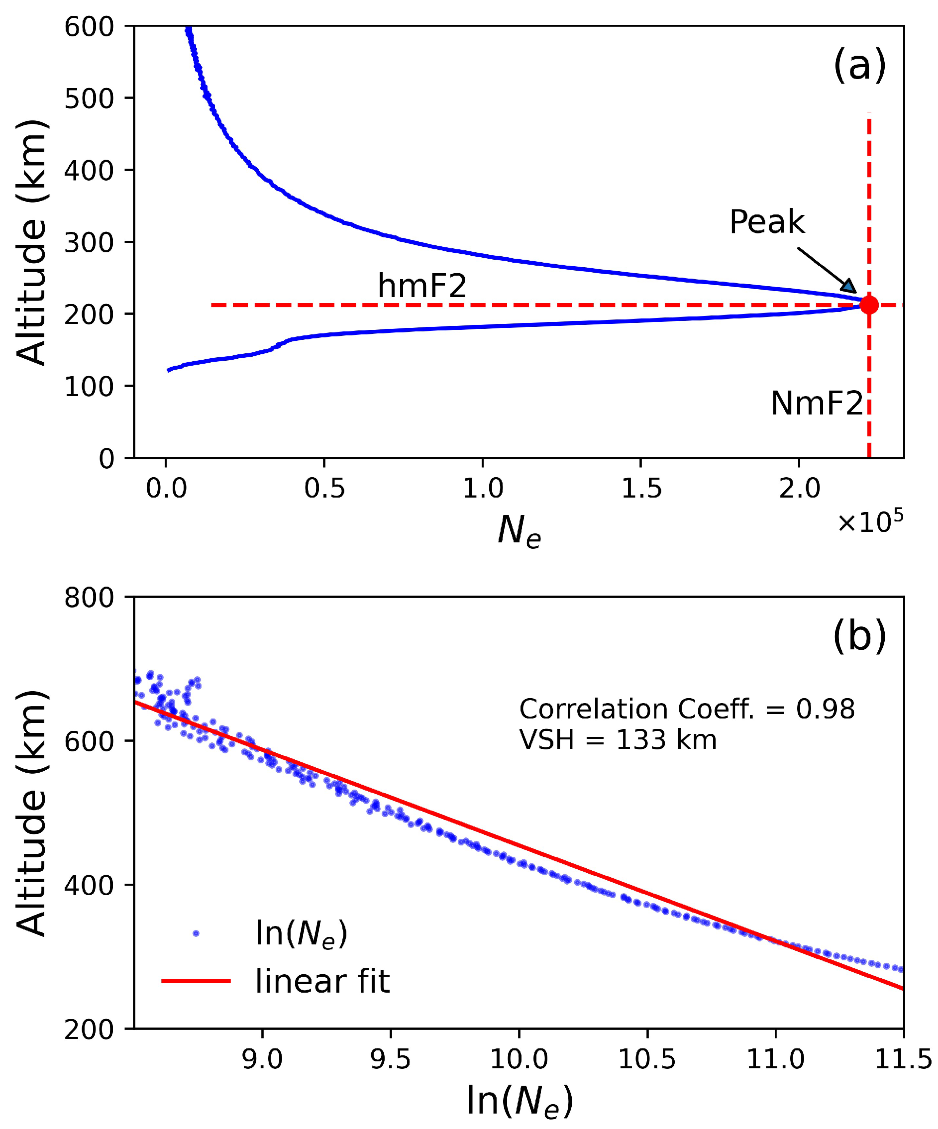
Figure 1 illustrates the definition of key topside ionospheric variables based on a typical N e profile. The x- and y-axes represent electron density and altitude, respectively. Figure 1a shows the peak value of the N e profile (NmF2) at the corresponding altitude (hmF2). In Figure 1b, the vertical scale height (VSH) is characterized by the N e decay in the topside ionosphere. The values of VSH are determined by d h / d ( ln ( N e ) ) at the lower topside layer [26]. The red line indicates the fitting result of N e profile.
Anomalies may occasionally occur in the N e profile. For example, due to energetic electron and proton precipitation ionization in the auroral region, an additional peak may appear below 200 km, which can be either higher or lower than the true F2 peak. In such cases, the peak search algorithm is constrained to the altitude range of 200–500 km, thereby effectively preventing the misidentification of hmF2 and NmF2. Note that each data point in the upper panel of Figure 1 represents an individual observation. It is treated as a separate sample in the N e modeling process, rather than using the entire profile as a single sample.
Therefore, the following criteria are applied to exclude profiles during data preprocessing: (1) profiles with a VSH correlation coefficient less than 0.85; (2) profiles with VSH greater than 400 km; and (3) profiles for which the peak cannot be identified within the altitude range.

3. Methodology

The overall structure of the L2-ANN follows the implementation described in Hu et al. [39]. The network parameters are initialized using the Xavier method [40]. The model includes three hidden layers, with activation functions of tanh, tanh, and sigmoid. Further details of the network architecture are provided in Appendix A. The input and output vairable sets are normalized to the range of [0, 1] before training using min–max scaling. The sigmoid activation in the output layer then produces outputs in [0, 1], which are subsequently denormalized back to physical units.
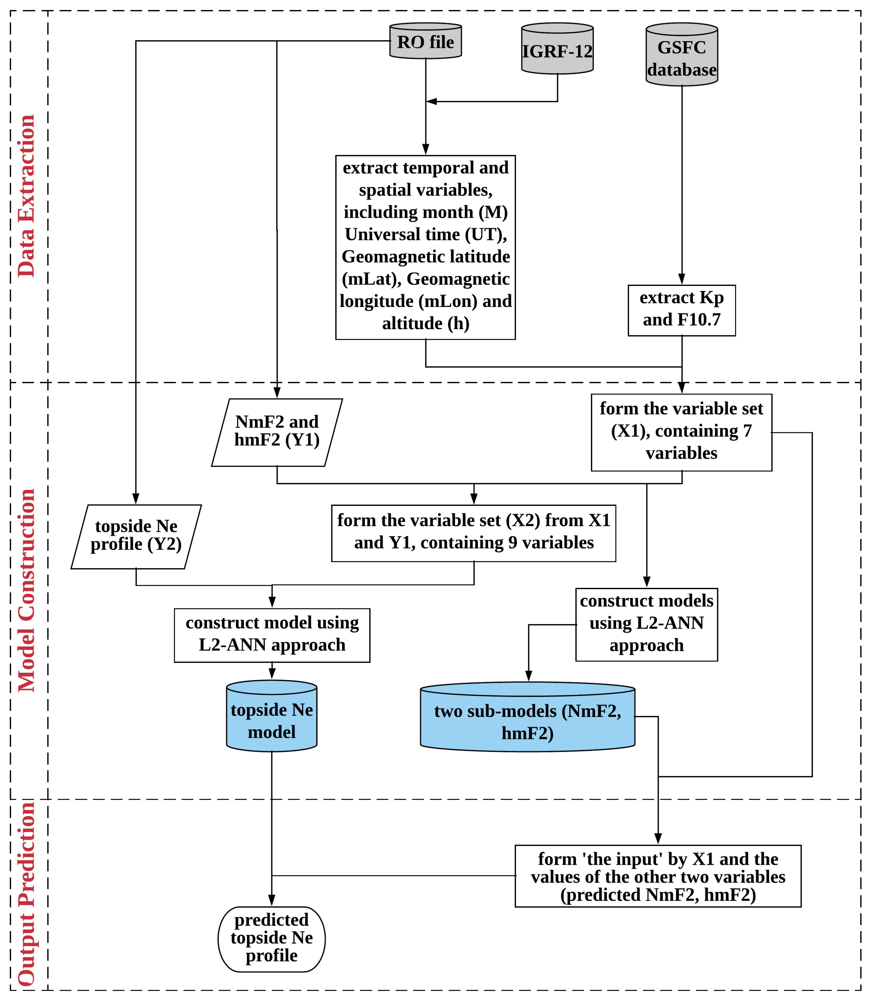
The construction of the four-dimensional topside N e model (see Figure 2) is carried out through a sequential procedure. The main steps are summarized as follows:
(1)
The initial input variable set X 1 is constructed. This set contains the first seven variables listed in Table 2. The corresponding observation set Y 1 consists of NmF2 and hmF2.
(2)
Two sub-models (NmF2 and hmF2) are developed to predict NmF2 and hmF2 using X 1 and Y 1 .
(3)
An extended input set X 2 is formed by combining X 1 and Y 1 . The corresponding output set Y 2 is defined as the topside N e .
(4)
The final topside N e model is constructed using X 2 and Y 2 .
Once the sub-models and the final N e model are trained, the framework can be used to predict electron density at a given location. The prediction procedure follows four steps:
(1)
The required input variables X 1 are extracted from available datasets or external models.
(2)
NmF2 and hmF2 are obtained to form Y 1 . When direct measurements are not available at the target location, these parameters are estimated using the two sub-models.
(3)
The extended input set X 2 is constructed using both X 1 and Y 1 .
(4)
The topside electron density N e is predicted using the trained L2-ANN model.
This two-stage modeling strategy allows the model to incorporate key physical characteristics of the ionosphere. In particular, NmF2 and hmF2 serve as intermediate variables that link bottomside observations with topside structure. By explicitly modeling these parameters, the framework reduces the dependence on direct measurements and improves its applicability in regions with limited observations.
The overall workflow of the modeling process, including data preparation, sub-model construction, and final prediction, is illustrated in Figure 2. Grey cylinders in the figure denote input datasets or existing models, while blue cylinders represent the outputs generated in this study. Rectangles indicate processing steps, and parallelograms represent intermediate data products.

4. Results

4.1. Data Selection

This study uses RO data from the COSMIC-1 and GRACE satellite missions. COSMIC-1 provides the most complete spatial and temporal coverage among the available datasets. A total of 3.2 million qualified COSMIC-1 profiles (“cosmic2013” processing mission) are selected as the primary dataset. These profiles correspond to the reprocessed COSMIC-1 observations.
After applying the data preprocessing criteria described in Section 2, approximately 9.63 × 10 8 valid N e samples are retained. Each sample corresponds to a single altitude point discretized from a N e profile. These samples span the period from 30 June 2007 to 30 April 2014. The remaining COSMIC-1 data, which are not used in training, form the out-of-sample testing dataset. The out-of-sample COSMIC-1 data, together with GRACE and ISR measurements, are used exclusively for model evaluation and validation. These datasets are independent of the training data, ensuring an unbiased assessment of the model’s performance.

4.2. Model Performance

Model performance is evaluated in terms of NmF2, hmF2, and topside N e .

4.2.1. Evaluation of NmF2 and hmF2

The accuracy of the NmF2 and hmF2 sub-models is assessed prior to evaluating the full N e model. Table 3 summarizes the comparison with IRI-2016. The IRI configuration includes the NeQuick2 topside model [41], the AMTB2013 (Altadill-Magdaleno-Torta-Blanch) hmF2 model [42], and the URSI-88 NmF2 model [43]. The evaluation is performed using out-of-sample COSMIC-1 data.
The evaluation metrics include the relative error and the root-mean-square error (RMSE), defined in Equations (1) and (2), respectively. The results indicate that the proposed sub-models show substantially better agreement with COSMIC-1 measurements than IRI-2016, with improvements of 4.5% and 11.0% for hmF2 and NmF2, respectively.
Relative error = 1 n | x ^ i x i | x ^ i ( i = 1 , , n ) ,
RMSE = 1 n ( x ^ i x i ) 2 ( i = 1 , , n ) ,
where x ^ i and x i denote the reference and predicted values, respectively, and n is the number of test samples.
The improvement is reasonable as both the training and testing datasets are derived from COSMIC-1, whereas IRI-2016 is constructed using heterogeneous data sources. Similar behavior has been reported in previous studies [44]. It is also worth noting that the URSI NmF2 models incorporate GNSS-RO data [45], although these updates are not yet fully implemented in IRI-2016.

4.2.2. Evaluation of Topside Electron Density

To quantify the contribution of each input variable, nine experimental schemes are designed (Table 4). Each scheme introduces additional variables to the model. This setup can be interpreted as a sensitivity analysis of the input feature set.
The results are summarized in Table 5. Both relative error and RMSE decrease significantly as more variables are included. Each successive scheme improves the performance by more than 20% compared with the previous one. This trend indicates that each variable contributes meaningful information to the model. It is worth noting that the rate of improvement decreases after Scheme 6 (which introduces K p ). The limited contribution of K p may result from the scarcity of geomagnetic disturbance events during the period from 2006 to 2017. The inclusion of NmF2 and hmF2 (Schemes 8 and 9) further improves the performance by 4% and 2%, respectively, indicating that these parameters provide additional information on the topside structure.
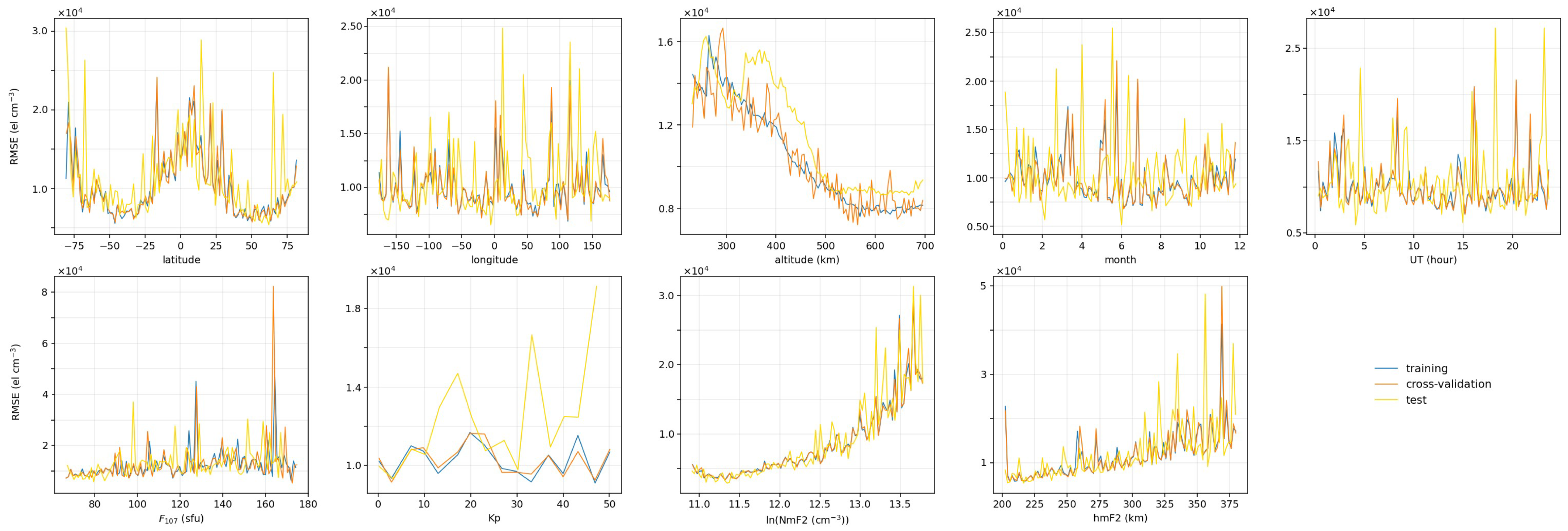
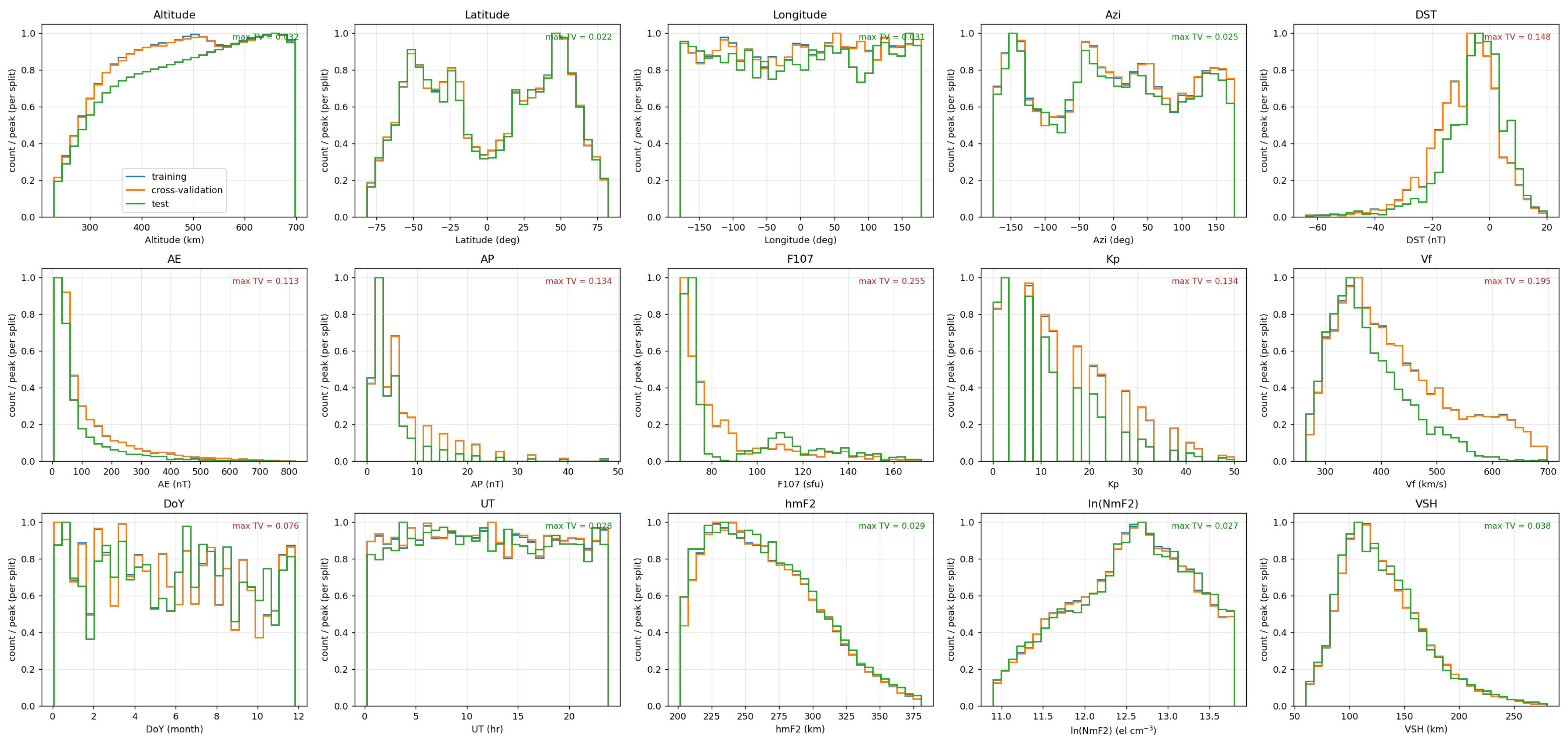
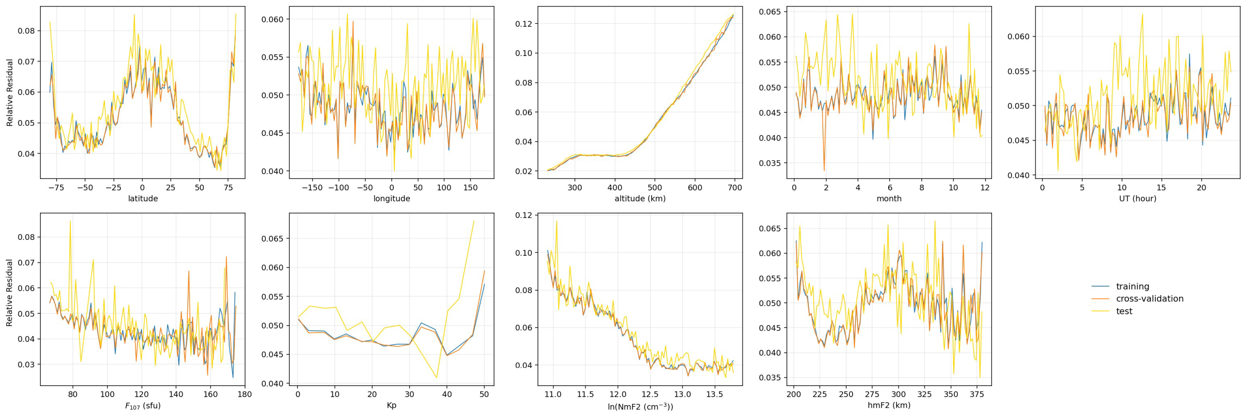
The robustness of the model is further evaluated using the training, validation, and testing datasets. Figure 3, Figure 4 and Figure 5 show the sample distributions and corresponding errors. The three datasets are mutually exclusive and are represented by different colors. The three datasets exhibit consistent distributions across all variables. This consistency confirms that no significant sampling bias is present. Furthermore, the error distributions are also similar across the three datasets. This result suggests that the model does not suffer from overfitting and maintains good generalization capability.
Several physical characteristics of model performance can be further identified:
(1)
The RMSE and relative errors are larger at high latitudes. This result reflects stronger ionospheric variability in these regions. Processes such as particle precipitation and Joule heating contribute to this variability, making accurate modeling more difficult.
(2)
In equatorial regions, the relative errors are smaller. However, the RMSE remains relatively large. This behavior is due to the higher absolute magnitude of N e in the EIA region. The EIA is characterized by two peaks in N e located on either side of the magnetic equator, which can reach values of up to 10 6 el/cm−3. As a result, even small relative errors can correspond to large absolute errors in these regions.
(3)
The relative errors decrease as NmF2 and hmF2 increase. This trend occurs because the overall magnitude of N e increases, while the absolute error remains relatively stable (see Figure 5).
(4)
During periods of solar maximum ( F 10.7 > 180 ) or enhanced geomagnetic activity (e.g., geomagnetic storms, K p > 5 ), both relative errors and RMSE exhibit increased variability, reflecting the intensified dynamics and nonlinear behavior of the ionosphere under disturbed conditions.
The final model is evaluated using independent datasets. Table 6 compares the proposed model with IRI-2016 using COSMIC-1, GRACE, and ISR data. Note that the model (with sub-models) is evaluated against COSMIC-1 out-of-sample data only, as this evaluation is intended solely to quantify the performance of NmF2 and hmF2 sub-model substitution relative to the recommended configuration using direct measurements. The results indicate that the proposed model substantially outperforms IRI-2016 across all reference datasets, highlighting the advantage of data-driven approaches in capturing complex nonlinear ionospheric structures.
When NmF2 and hmF2 are not directly available, the sub-models are used to estimate these parameters (referred to as the “with sub-models” configuration). Table 6 shows that this configuration introduces additional uncertainty by 19.4% compared with the baseline model. However, it remains 15.6% better than IRI-2016. This result indicates that the overall framework with and without the sub-models remains robust.
In addition, the best performance is achieved with respect to out-of-sample COSMIC-1 data, while the largest error occurs for ISR data. This difference likely reflects the higher precision and localized nature of ISR measurements. The higher relative error for ISR data underscores the challenges in modeling localized ionospheric features. The improved performance of the model is partly influenced by the use of COSMIC-1 data in both training and testing. In contrast, IRI-2016 is constructed from heterogeneous data sources. Similar findings have been reported by Sai Gowtam and Tulasi Ram [44].
It should be noted that the training and evaluation datasets used in this study (2007–2014) are predominantly characterized by quiet to weakly disturbed solar and geomagnetic conditions. Under such conditions, the F2-layer peak height (hmF2) rarely exceeds 500 km (Figure 3). Consequently, the model’s performance and conclusions are robust within this regime. However, during intense solar storms or in specific equatorial regions, hmF2 can occasionally rise above 500 km. The current model, trained exclusively on data with hmF2 ≤ 500 km, may exhibit increased bias under such extreme events. Future work will extend the model by including storm-time data and relaxing the hmF2 constraint to improve its applicability under extreme space weather conditions.

5. Discussion

The results in Section 4.2 demonstrate the statistical performance of the proposed model. In this section, the focus shifts to the physical consistency of the modeled N e . The aim is to further assess whether the new models can reproduce key physical features of the ionosphere under different geophysical conditions.
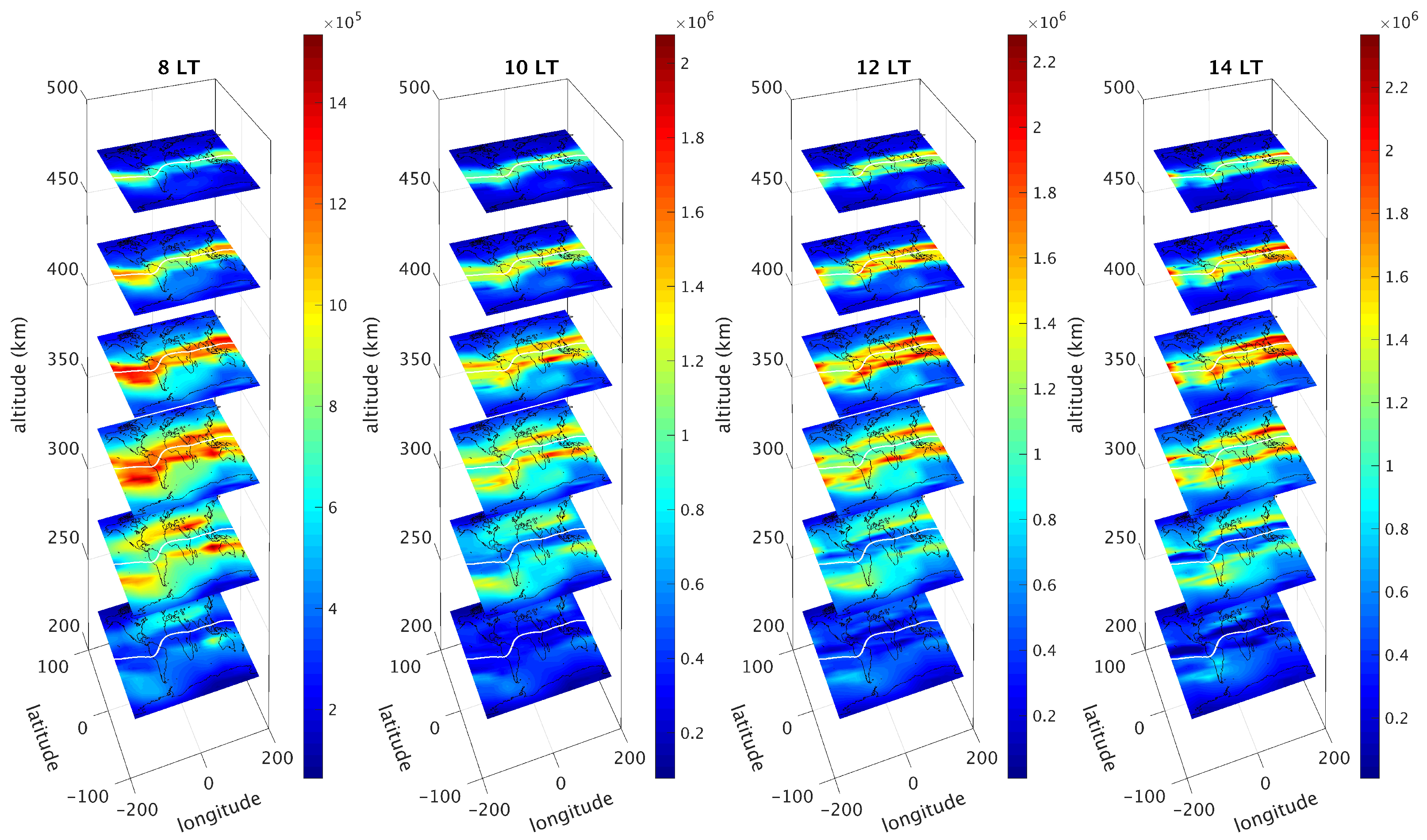
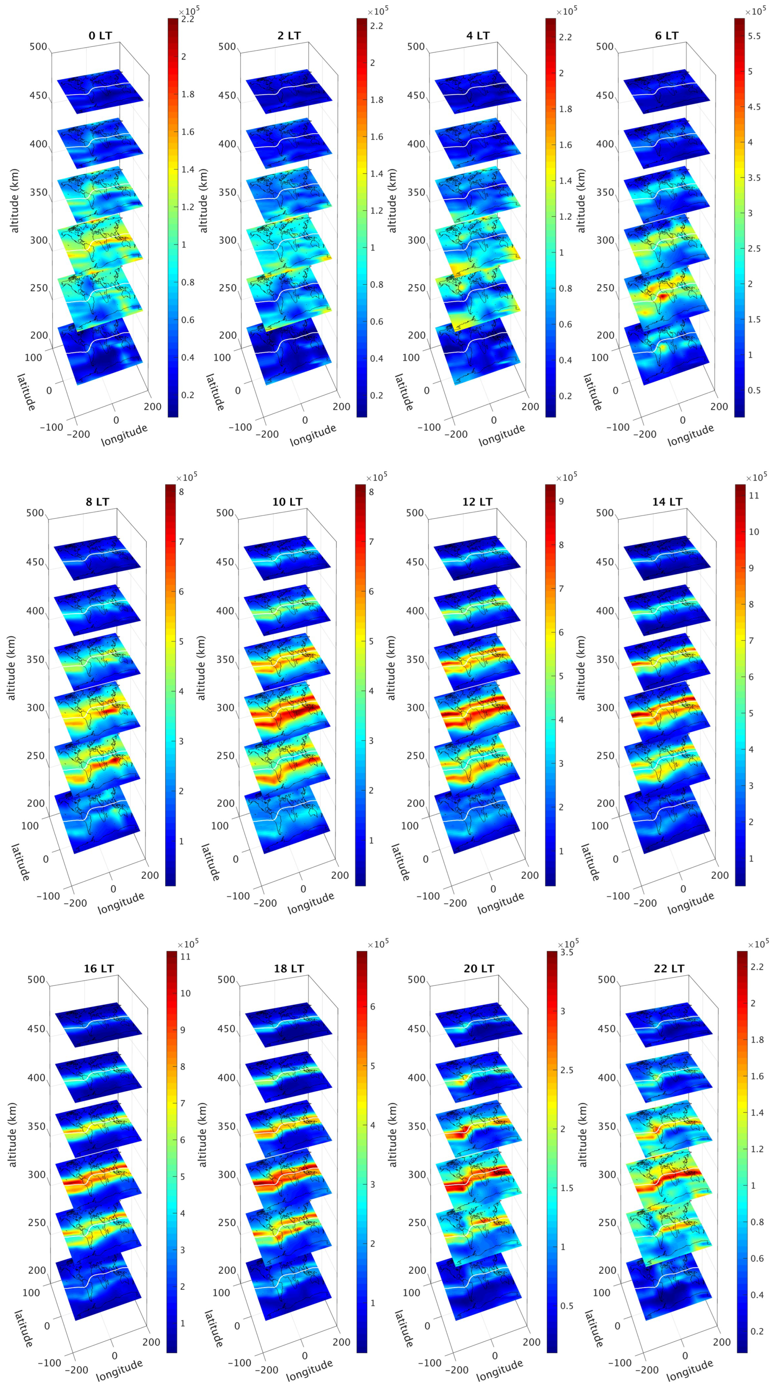
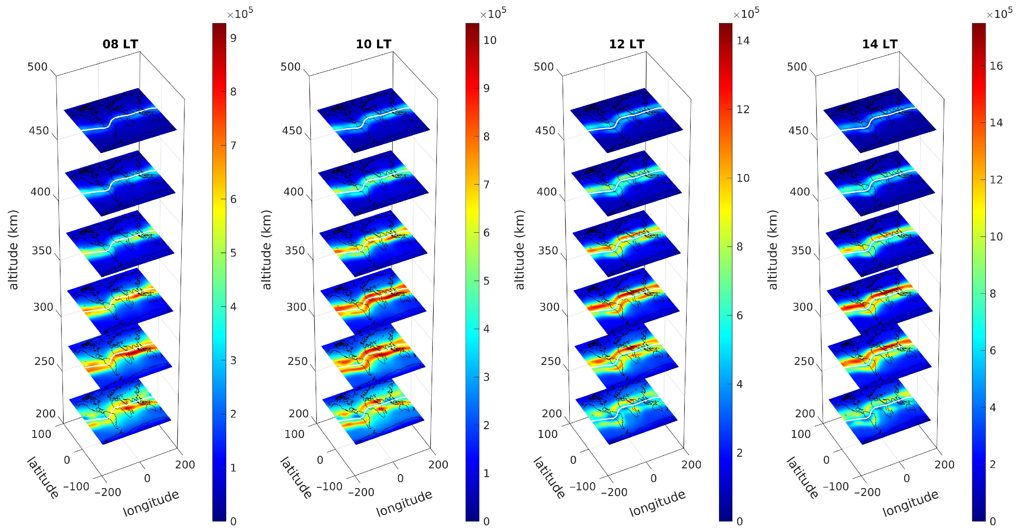
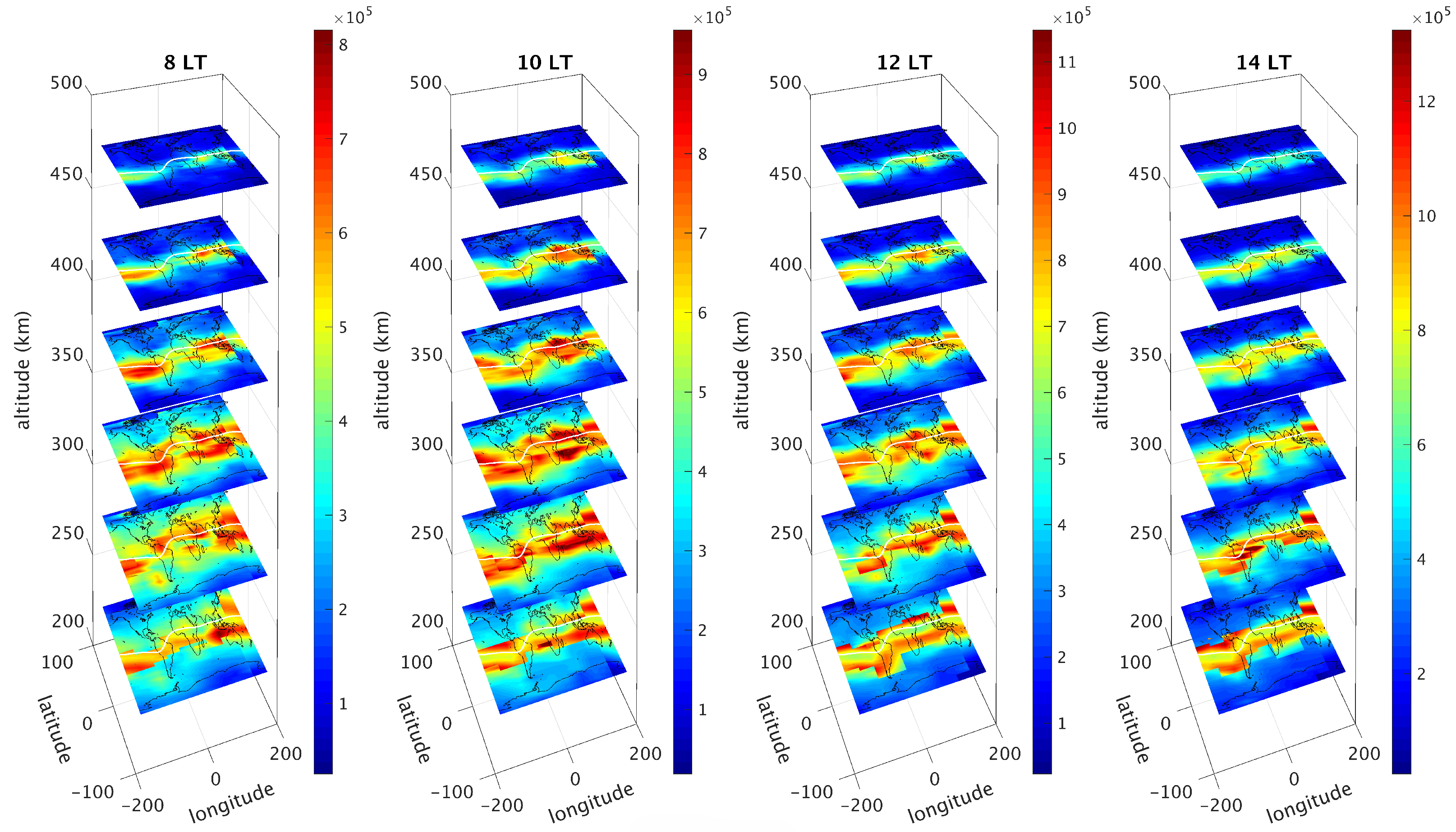
Figure 6 presents global distributions of N e at different local times on the September equinox under solar minimum conditions. The altitude and temporal resolutions are 50 km and 2 h, respectively. It should be noted that, although the focus of this study is on the topside ionosphere, the bottomside N e is included for completeness. The new model clearly reproduces the EIA feature. It develops between approximately 08 and 18 local time, which is consistent with established ionospheric behavior. Figure 7 presents the EIA and MSNA features as reproduced by IRI-2016. The comparison clearly shows that while IRI-2016 captures the gross morphology, it underestimates both the EIA and the MSNA under certain solar conditions. In contrast, our model reproduces these features with substantially higher fidelity.
A comparison with COSMIC-1 observations (Figure 8) shows that the modeled EIA structure is more clearly defined. This difference arises because COSMIC-1 maps are constructed from monthly averaged measurements to ensure sufficient spatial coverage, which tends to smooth localized features. In contrast, the model effectively reconstructs the underlying spatial structures, further demonstrating its capability to capture key ionospheric characteristics.
Figure 9 shows the model results under solar maximum conditions. A clear enhancement in N e is observed compared to the solar minimum case, indicating a strong positive correlation between electron density and solar activity. In addition, the modeled N e decreases with increasing altitude in the topside ionosphere, which is consistent with the expected physical behavior governed by diffusive equilibrium.
Previous studies have reported an MSNA feature [46]. This phenomenon is characterized by a noon-time minimum and an evening maximum in the diurnal variation of N e . It occurs in the Northern Hemisphere during the June solstice and in the Southern Hemisphere during the December solstice. This phenomenon is also known as the Weddell Sea Anomaly, occurring over Antarctica and the adjacent Pacific region.
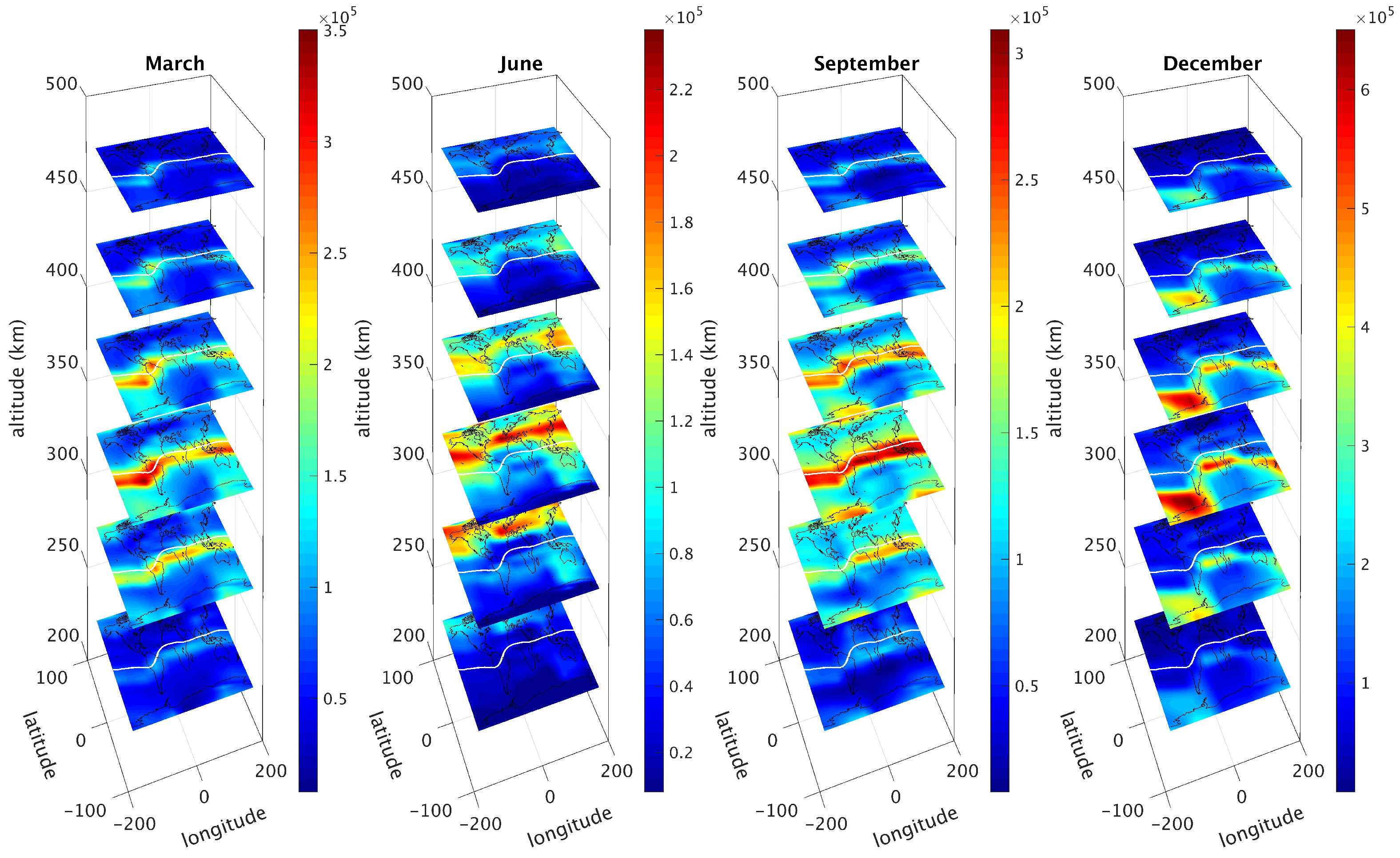
Figure 10 shows the modeled N e at 22 local time for different seasons. The MSNA is clearly reproduced during the June solstice. The Weddell Sea Anomaly (i.e., December MSNA) is well represented during the December solstice. These findings indicate that the new model successfully inherits key physical characteristics from the COSMIC-1 observations and is capable of reproducing complex seasonal and diurnal ionospheric phenomena.
While the proposed model demonstrates clear statistical improvements over IRI-2016, the underlying reasons for its superior performance are not fully understood. A more in-depth diagnostic analysis—such as comparing the VSH and the longitudinal variations in the EIA between the ANN model and IRI-2016—would help open the “black box” in the ANN model and identify the specific sources of improvement. For instance, it remains to be examined whether the ANN better captures the altitude-dependent increase in VSH or the wave-number-4 longitudinal structure associated with non-migrating tides. These questions are beyond the scope of the current study but represent important directions for future work. Addressing them will not only enhance the interpretability of the ANN model but also provide deeper insights into the physical processes governing topside ionospheric variability.

6. Conclusions

This study developed a novel four-dimensional topside N e model based on COSMIC-1 satellite-to-satellite limb-sounding measurements (GNSS-RO) using the L2-regularized deep learning approach. The model integrates a comprehensive suite of physical and empirical ionospheric variables, the individual contributions of which were systematically evaluated. The performance of the proposed model was rigorously validated against the IRI-2016 model using out-of-sample COSMIC-1 data, as well as independent GRACE and ISR measurements. The primary conclusions are summarized as follows:
  • The results demonstrate clear improvements over IRI-2016. The sub-models reduce relative errors by 4.5% for hmF2 and 11.0% for NmF2. The full N e model achieves improvements of 35%, 36%, and 53% when evaluated against COSMIC-1, GRACE, and ISR datasets, respectively.
  • The analysis also shows that spatial and temporal variables, together with NmF2, hmF2, and solar and geomagnetic indices ( F 10.7 and K p ), play key roles in determining model performance.
  • The model retained the characteristics of COSMIC-1 measurements under both low and high solar activity conditions, accurately reproducing the Equatorial Ionization Anomaly (EIA) and Midlatitude Summer Nighttime Anomaly (MSNA).
  • The model showed better agreement with GRACE than ISR data (relative errors: 12.4% and 24.3%), suggesting GRACE data quality is comparable to COSMIC-1 for this application. Future GNSS-RO missions are thus promising sources for enhancing topside N e modeling.
Future work will explore more advanced deep learning architectures, including convolutional neural networks, recurrent neural networks, and self-attention mechanisms, in topside ionosphere modeling. These approaches may better capture spatial and temporal dependencies. Additional GNSS-RO datasets will also be incorporated to further improve model generalization.

Author Contributions

Conceptualization, A.H. and C.H.; methodology, A.H.; software, A.H. and C.H.; validation, C.H., A.H. and H.C.; formal analysis, C.H. and A.H.; data curation, A.H.; writing: C.H., A.H. and H.C.; visualization, A.H. and C.H.; supervision, C.H., Z.X. and D.Z.; funding acquisition, C.H., Z.X. and D.Z. All authors have read and agreed to the published version of the manuscript.

Funding

This research was funded by the National Natural Science Foundation of China (NSFC) (No. 42204037, 42504029), the Natural Science Foundation of Hunan Province, China (No. 2026JJ80797), and the Research Foundation of Education Bureau of Hunan Province, China (No. 25B0437).

Data Availability Statement

The COSMIC-1 ionPrf data used in this study are provided by UCAR/CDAAC (https://data.cosmic.ucar.edu/gnss-ro/cosmic1/repro2013/level2, accessed on 12 April 2019), the K p and F 10.7 data can be downloaded from OMNIWeb (https://omniweb.gsfc.nasa.gov/, accessed on 12 April 2019), and the ISR measurements can be obtained from the Madrigal database (http://cedar.openmadrigal.org, accessed on 12 April 2019). The new topside N e model and two sub-models (NmF2 and hmF2) developed in this study are available on the website Zenodo (https://doi.org/10.5281/zenodo.2657358).

Acknowledgments

The authors are grateful to the reviewers for their constructive suggestions on this article. During the preparation of this manuscript/study, the authors used OpenAI’s ChatGPT (GPT-5) for language editing and grammatical refinement. The authors have reviewed and edited the output and take full responsibility for the content of this publication.

Conflicts of Interest

The authors declare no conflicts of interest.

Abbreviations

The following abbreviations are used in this manuscript:
COSMICConstellation Observing System for Meteorology, Ionosphere, and Climate
EIAEquatorial Ionization Anomaly
GNSSGlobal Navigation Satellite System
IRIInternational Reference Ionosphere
ISRIncoherent Scatter Radar
MSNAMid-Latitude Summer Nighttime Anomaly
RMSERoot-Mean-Square Error
RORadio Occultation
UTUniversal Time
VSHVertical Scale Height

Appendix A. Neural Network System

A neural network is a class of algorithms designed to identify the underlying relationships between dependent and independent variables by mimicking the information processing mechanisms of the human brain. A general neural network training procedure typically consists of the following five steps [47]:
(1)
Weights ( Θ ) initialization using the Xavier method [40];
(2)
Forward propagation (computation of a and z) as shown in Figure A1;
(3)
Cost function (J) evaluation;
(4)
Backward propagation (computation of d a , d z , and d Θ );
(5)
Weight update, followed by iteration from Step (2) until convergence of the cost function.

Appendix A.1. Initialization and Forward Propagation
The Xavier initialization method, proposed by Glorot and Bengio [40] and further analyzed by He et al. [48], is widely used to improve training stability, particularly for networks with a relatively small number of input features (e.g., fewer than 20). The initialization is given by
Θ l = 2 p i n + p o u t ,
where p i n and p o u t denote the numbers of input and output units in the lth layer, respectively, and Θ l represents the parameter set associated with that layer (see Figure A1).
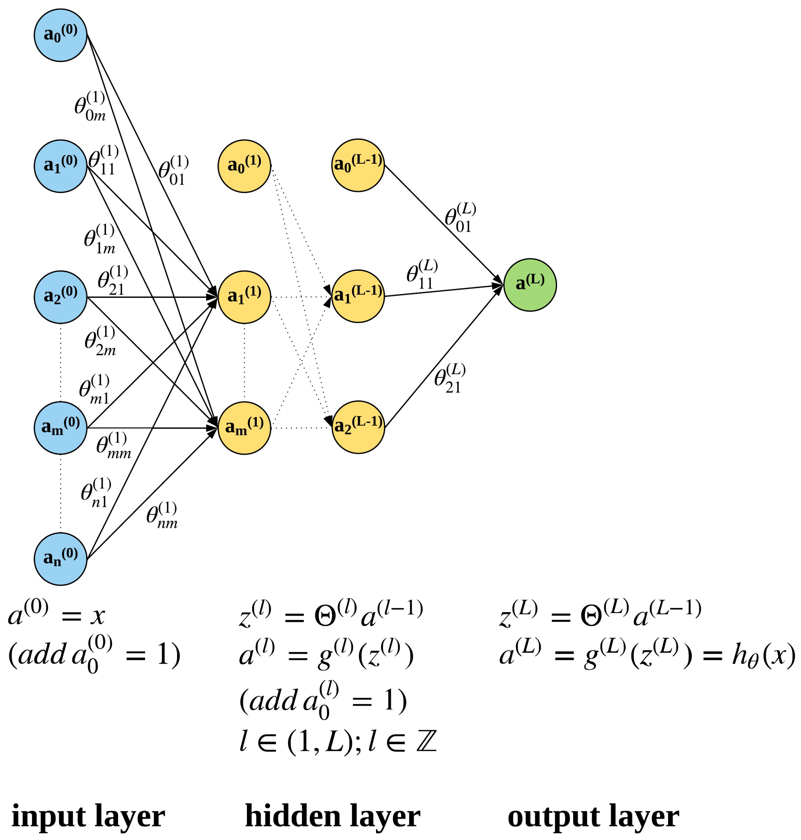
The architecture of the artificial neural network (ANN) employed in this study is illustrated in Figure A1, comprising input, hidden, and output layers. Multiple sub-layers may exist within the hidden layer. The equations shown in the figure describe the Step (2) forward propagation process, in which the input x is mapped to the output h θ ( x ) through successive linear transformations and nonlinear activation functions. During backward propagation, mini-batch gradient descent [49] is used to optimize Θ by minimizing the cost function J.
The activation function g ( l ) for the lth layer introduces nonlinearity into the model. Common choices include the rectified linear unit (ReLU), hyperbolic tangent (tanh), and sigmoid functions, defined as
ReLU ( x ) = m a x ( 0 , x ) , tanh ( x ) = e x + e x e x e x , sigmoid ( x ) = 1 1 + e x .
Figure A1. Structure of a three-layer ANN: input (blue), hidden (yellow), and output (green) layers. The variables a denote neuron values, with superscripts indicating layer indices and subscripts indicating neuron indices. The terms a 0 ( l ) represent bias units in each layer. Θ ( l ) denotes the set of weights connecting the ( l 1 ) th and lth layers, and θ n m ( l ) represents the weight between the nth neuron in the ( l 1 ) th layer and the mth neuron in the lth layer. The variables x and h θ ( x ) denote the input and output of the model, respectively, and g ( l ) is the activation function for the lth layer.
Remotesensing 18 02002 g0a1

Appendix A.2. L2-Regularized ANN

A common limitation of traditional neural networks is their susceptibility to overfitting or underfitting [50], particularly when shallow architectures are employed. Regularization techniques are commonly used to mitigate this issue [51]. In this study, L2 regularization [52] is adopted.
The L2-regularized cost function in Step (3) for the qth output neuron is defined as
J ( q ) = 1 2 k i = 1 k y ( q ) [ i ] h θ ( q ) [ i ] ( x ) 2 regular   J + 1 k λ 2 ( θ ( q ) ) 2 L 2 - regularized   cost ( J L 2 ) ,
where λ is the regularization parameter and k is the number of training samples. The variable y represents the observed value of the dependent variable (i.e., N e in this study), and q = 1 denotes the index of the outputs. The dropout approach (another commonly used technique) is not adopted in this study, as it demonstrates inferior performance in this application.
During backward propagation, the gradient of the L2-regularized cost function introduces an additional penalty term to the standard gradient d Θ , consistent with Hu et al. [39]. The gradient descent procedure follows the same implementation as described in Hu et al. [39].
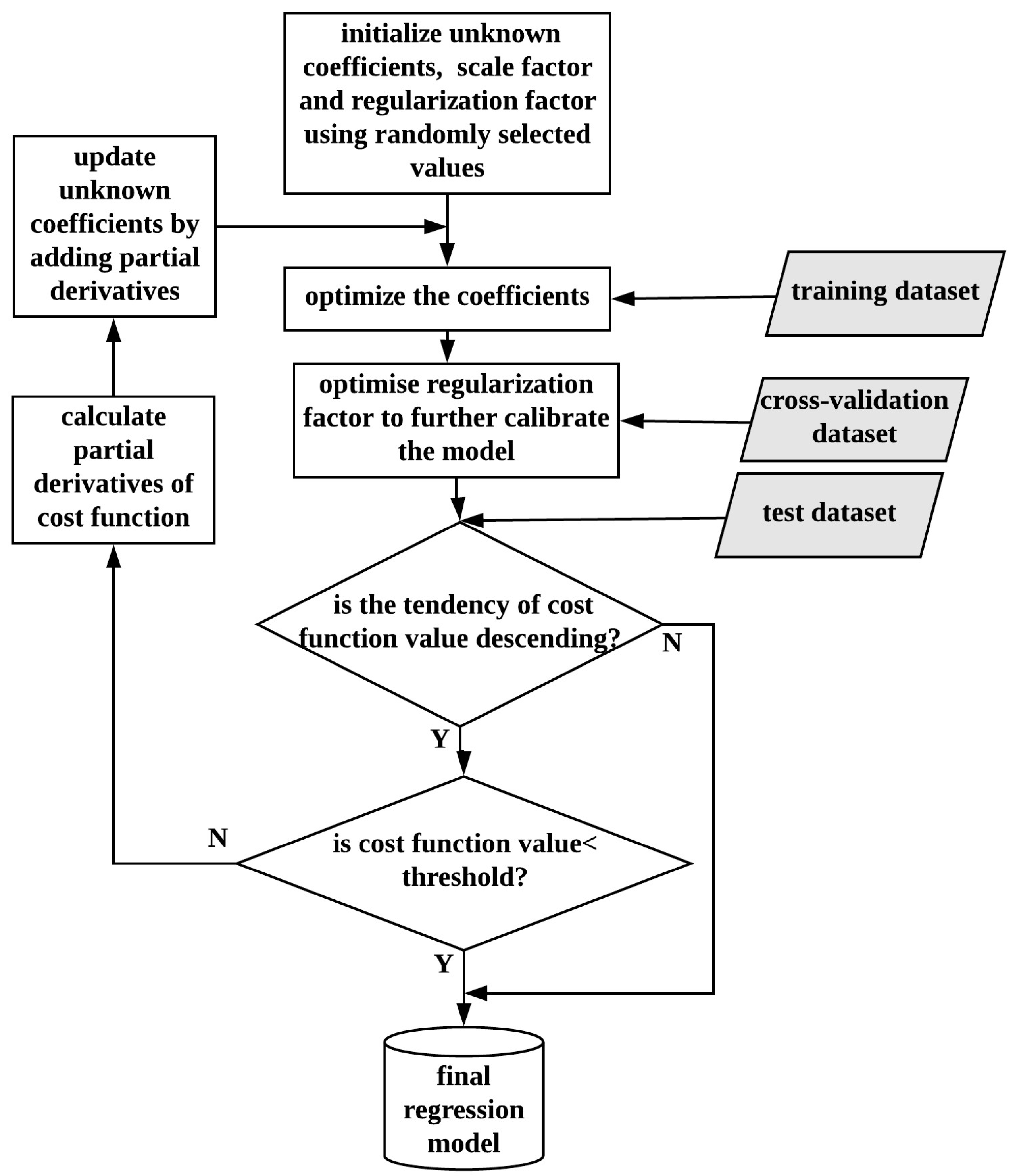
After training, a cross-validation dataset is used to determine the optimal value of λ . The flowchart of the overall L2-regularized ANN procedure is shown in Figure A2. The network adopted in this study consists of three hidden layers, with 16, 16, and 8 neurons, respectively. The corresponding activation functions are tanh, tanh, and sigmoid. This configuration is selected based on empirical experience, balancing model accuracy and computational efficiency.
Figure A2. Flowchart illustrating the ANN-based regression modeling procedure. Grey parallelograms represent the datasets used at different stages, white rectangles denote processing steps, white diamonds indicate decision points controlling the workflow, and the cylinder represents the final ANN-derived regression model.
Remotesensing 18 02002 g0a2

References

  1. Farley, D., Jr. A plasma instability resulting in field-aligned irregularities in the ionosphere. J. Geophys. Res. 1963, 68, 6083–6097. [Google Scholar] [CrossRef]
  2. Liu, L.; He, M.; Wan, W.; Zhang, M.L. Topside ionospheric scale heights retrieved from Constellation Observing System for Meteorology, Ionosphere, and Climate radio occultation measurements. J. Geophys. Res. Space Phys. 2008, 113, A10304. [Google Scholar] [CrossRef]
  3. Shim, J.; Kuznetsova, M.; Rastätter, L.; Hesse, M.; Bilitza, D.; Butala, M.; Codrescu, M.; Emery, B.; Foster, B.; Fuller-Rowell, T.; et al. CEDAR electrodynamics thermosphere ionosphere (ETI) challenge for systematic assessment of ionosphere/thermosphere models: NmF2, hmF2, and vertical drift using ground-based observations. Space Weather 2011, 9, 12. [Google Scholar] [CrossRef]
  4. Hoque, M.M.; Jakowski, N. Higher order ionospheric effects in precise GNSS positioning. J. Geod. 2007, 81, 259–268. [Google Scholar]
  5. Hu, A.; Li, Z.; Carter, B.; Wu, S.; Wang, X.; Norman, R.; Zhang, K. Helmert-VCE-aided fast-WTLS approach for global ionospheric VTEC modelling using data from GNSS, satellite altimetry and radio occultation. J. Geod. 2018, 93, 877–888. [Google Scholar] [CrossRef]
  6. Pullen, S.; Park, Y.S.; Enge, P. Impact and mitigation of ionospheric anomalies on ground-based augmentation of GNSS. Radio Sci. 2009, 44, 1–10. [Google Scholar] [CrossRef]
  7. Dyson, P.L.; Benson, R.F. Topside sounder observations of equatorial bubbles. Geophys. Res. Lett. 1978, 5, 795–798. [Google Scholar] [CrossRef]
  8. Thome, G.D. Incoherent scatter observations of traveling ionospheric disturbances. J. Geophys. Res. 1964, 69, 4047–4049. [Google Scholar] [CrossRef]
  9. Lei, J.; Liu, L.; Wan, W.; Zhang, S.R. Variations of electron density based on long-term incoherent scatter radar and ionosonde measurements over Millstone Hill. Radio Sci. 2005, 40, 1–10. [Google Scholar] [CrossRef]
  10. Richards, P.; Meier, R.; Wilkinson, P. On the consistency of satellite measurements of thermospheric composition and solar EUV irradiance with Australian ionosonde electron density data. J. Geophys. Res. Space Phys. 2010, 115, A10309. [Google Scholar] [CrossRef]
  11. Bilitza, D. A correction for the IRI topside electron density model based on Alouette/ISIS topside sounder data. Adv. Space Res. 2004, 33, 838–843. [Google Scholar] [CrossRef]
  12. Yue, X.; Schreiner, W.S.; Lin, Y.C.; Rocken, C.; Kuo, Y.H.; Zhao, B. Data assimilation retrieval of electron density profiles from radio occultation measurements. J. Geophys. Res. Space Phys. 2011, 116, A03317. [Google Scholar] [CrossRef]
  13. Sokolovskiy, S.; Rocken, C. Algorithms for Inverting Radio Occultation Signals in the Neutral Atmosphere; University Corporation for Atmospheric Research: Boulder, CO, USA, 2006. [Google Scholar]
  14. Lei, J.; Syndergaard, S.; Burns, A.G.; Solomon, S.C.; Wang, W.; Zeng, Z.; Roble, R.G.; Wu, Q.; Kuo, Y.H.; Holt, J.M.; et al. Comparison of COSMIC ionospheric measurements with ground-based observations and model predictions: Preliminary results. J. Geophys. Res. Space Phys. 2007, 112, A07308. [Google Scholar] [CrossRef]
  15. Ho, S.P.; Anthes, R.A.; Ao, C.O.; Healy, S.; Horanyi, A.; Hunt, D.; Mannucci, A.J.; Pedatella, N.; Randel, W.J.; Simmons, A.; et al. The COSMIC/FORMOSAT-3 Radio Occultation Mission after 12 Years: Accomplishments, Remaining Challenges, and Potential Impacts of COSMIC-2. Bull. Am. Meteorol. Soc. 2020, 101, E1107–E1136. [Google Scholar] [CrossRef]
  16. Li, W.; Li, J.; Meng, X.; Zhao, D.; He, C.; Zuo, X.; Zhang, K. A deep learning model for correcting nonlinear biases between the TEC measurements of COSMIC-2 and GNSS. Adv. Space Res. 2025, 76, 3768–3783. [Google Scholar] [CrossRef]
  17. Krankowski, A.; Zakharenkova, I.; Krypiak-Gregorczyk, A.; Shagimuratov, I.I.; Wielgosz, P. Ionospheric electron density observed by FORMOSAT-3/COSMIC over the European region and validated by ionosonde data. J. Geod. 2011, 85, 949–964. [Google Scholar] [CrossRef]
  18. Seba, E.B.; Jacobs, C.; Melcot, M.; Poedts, S. Evaluation of COSMIC-2 satellite data for foF2 and hmF2 against ground-based ionosondes and the PyIRI (2020) model across middle to low latitudes. Space Weather 2026, 24, e2024SW004321. [Google Scholar] [CrossRef]
  19. Reinisch, B.; Nsumei, P.; Huang, X.; Bilitza, D. Modeling the F2 topside and plasmasphere for IRI using IMAGE/RPI and ISIS data. Adv. Space Res. 2007, 39, 731–738. [Google Scholar] [CrossRef]
  20. Bilitza, D.; Pezzopane, M.; Truhlik, V.; Altadill, D.; Reinisch, B.W.; Pignalberi, A. The International Reference Ionosphere Model: A Review and Description of an Ionospheric Benchmark. Rev. Geophys. 2022, 60, e2022RG000792. [Google Scholar] [CrossRef]
  21. Pezzopane, M.; Pignalberi, A.; Nava, B. On the low-latitude NeQuick topside ionosphere mismodelling: The role of parameters H0, g, and r. Adv. Space Res. 2023, 72, 1224–1236. [Google Scholar] [CrossRef]
  22. Pignalberi, A.; Bilitza, D.; Coïsson, P.; Haralambous, H.; Nava, B.; Pezzopane, M.; Prol, F.; Smirnov, A.; Themens, D.R.; Xiong, C. Validation of the IRI-2020 topside ionosphere options through in-situ electron density observations by low-Earth-orbit satellites. Adv. Space Res. 2025, 75, 4192–4216. [Google Scholar] [CrossRef]
  23. Bilitza, D.; Xiong, C. A solar activity correction term for the IRI topside electron density model. Adv. Space Res. 2021, 68, 2124–2137. [Google Scholar] [CrossRef]
  24. Smirnov, A.; Shprits, Y.; Prol, F.; Lühr, H.; Berrendorf, M.; Zhelavskaya, I.; Xiong, C. A novel neural network model of Earth’s topside ionosphere. Sci. Rep. 2023, 13, 1303. [Google Scholar] [CrossRef] [PubMed]
  25. Burns, A.; Solomon, S.; Wang, W.; Qian, L.; Zhang, Y.; Paxton, L. Daytime climatology of ionospheric NmF2 and hmF2 from COSMIC data. J. Geophys. Res. Space Phys. 2012, 117, A09315. [Google Scholar] [CrossRef]
  26. Liu, L.; Le, H.; Wan, W.; Sulzer, M.P.; Lei, J.; Zhang, M.L. An analysis of the scale heights in the lower topside ionosphere based on the Arecibo incoherent scatter radar measurements. J. Geophys. Res. Space Phys. 2007, 112, A06307. [Google Scholar] [CrossRef]
  27. Richards, P. Seasonal and solar cycle variations of the ionospheric peak electron density: Comparison of measurement and models. J. Geophys. Res. Space Phys. 2001, 106, 12803–12819. [Google Scholar] [CrossRef]
  28. Zheng, D.; Yao, Y.; Nie, W.; Chu, N.; Lin, D.; Ao, M. A new three-dimensional computerized ionospheric tomography model based on a neural network. GPS Solut. 2021, 25, 10. [Google Scholar]
  29. Ren, X.; Yang, P.; Liu, H.; Chen, J.; Liu, W. Deep learning for global ionospheric TEC forecasting: Different approaches and validation. Space Weather 2022, 20, e2021SW003011. [Google Scholar] [CrossRef]
  30. Li, W.; Zhu, H.; Yang, F.; Wen, C.; Shi, S.; Zhao, D.; He, C.; Li, Z. Storm-time ionospheric model over Yunnan-Sichuan area of China based on the SSA-ConvLSTM-BiLSTM algorithm. GPS Solut. 2025, 29, 77. [Google Scholar] [CrossRef]
  31. Lin, Y.; Fang, H.; Duan, D.; Huang, H.; Xiao, C.; Ren, G.; Li, C.; Zhou, C. Enhancing Deep Learning Ionospheric Modeling with Solar Radiation and Flare Classes. J. Geophys. Res. Space Phys. 2025, 130, e2024JA033319. [Google Scholar] [CrossRef]
  32. Rocken, C.; Anthes, R.; Exner, M.; Hunt, D.; Sokolovskiy, S.; Ware, R.; Gorbunov, M.; Schreiner, W.; Feng, D.; Herman, B.; et al. Analysis and validation of GPS/MET data in the neutral atmosphere. J. Geophys. Res. Atmos. 1997, 102, 29849–29866. [Google Scholar] [CrossRef]
  33. Hajj, G.A.; Romans, L.J. Ionospheric electron density profiles obtained with the Global Positioning System: Results from the GPS/MET experiment. Radio Sci. 1998, 33, 175–190. [Google Scholar] [CrossRef]
  34. Schreiner, W.; Rocken, C.; Sokolovskiy, S.; Syndergaard, S.; Hunt, D. Estimates of the precision of GPS radio occultations from the COSMIC/FORMOSAT-3 mission. Geophys. Res. Lett. 2007, 34, L04808. [Google Scholar] [CrossRef]
  35. Beyerle, G.; Schmidt, T.; Michalak, G.; Heise, S.; Wickert, J.; Reigber, C. GPS radio occultation with GRACE: Atmospheric profiling utilizing the zero difference technique. Geophys. Res. Lett. 2005, 32, L13806. [Google Scholar] [CrossRef]
  36. Zhang, S.; Holt, J.M.; Zalucha, A.M.; AmoryMazaudier, C. Midlatitude ionospheric plasma temperature climatology and empirical model based on Saint Santin incoherent scatter radar data from 1966 to 1987. J. Geophys. Res. Space Phys. 2004, 109, A11311. [Google Scholar] [CrossRef]
  37. Lei, J.; Roble, R.G.; Wang, W.; Emery, B.A.; Zhang, S.R. Electron temperature climatology at Millstone Hill and Arecibo. J. Geophys. Res. Space Phys. 2007, 112, A02302. [Google Scholar] [CrossRef]
  38. Drob, D.P.; Emmert, J.T.; Meriwether, J.W.; Makela, J.J.; Doornbos, E.; Conde, M.; Hernandez, G.; Noto, J.; Zawdie, K.A.; McDonald, S.E.; et al. An update to the Horizontal Wind Model (HWM): The quiet time thermosphere. Earth Space Sci. 2015, 2, 301–319. [Google Scholar] [CrossRef]
  39. Hu, A.; Wu, S.; Wang, X.; Wang, Y.; Norman, R.; He, C.; Cai, H.; Zhang, K. Improvement of Reflection Detection Success Rate of GNSS RO Measurements Using Artificial Neural Network. IEEE Trans. Geosci. Remote Sens. 2018, 56, 760–769. [Google Scholar] [CrossRef]
  40. Glorot, X.; Bengio, Y. Understanding the difficulty of training deep feedforward neural networks. In Proceedings of the Thirteenth International Conference on Artificial Intelligence and Statistics, Sardinia, Italy, 13–15 May 2010; pp. 249–256. [Google Scholar]
  41. Nava, B.; Coisson, P.; Radicella, S. A new version of the NeQuick ionosphere electron density model. J. Atmos. Sol.-Terr. Phys. 2008, 70, 1856–1862. [Google Scholar] [CrossRef]
  42. Altadill, D.; Magdaleno, S.; Torta, J.; Blanch, E. Global empirical models of the density peak height and of the equivalent scale height for quiet conditions. Adv. Space Res. 2013, 52, 1756–1769. [Google Scholar] [CrossRef]
  43. Rush, C. URSI foF2model maps (1988). Planet. Space Sci. 1992, 40, 546–547. [Google Scholar] [CrossRef]
  44. Sai Gowtam, V.; Tulasi Ram, T. An Artificial Neural Network-Based Ionospheric Model to Predict NmF2 and hmF2 Using Long-Term Data Set of FORMOSAT-3/COSMIC Radio Occultation Observations: Preliminary Results. J. Geophys. Res. Space Phys. 2017, 122, 743–755. [Google Scholar] [CrossRef]
  45. Hoque, M.; Jakowski, N. A new global model for the ionospheric F2 peak height for radio wave propagation. Ann. Geophys. 2012, 30, 797–809. [Google Scholar] [CrossRef]
  46. Lin, C.; Liu, C.; Liu, J.; Chen, C.; Burns, A.; Wang, W. Midlatitude summer nighttime anomaly of the ionospheric electron density observed by FORMOSAT-3/COSMIC. J. Geophys. Res. Space Phys. 2010, 115, A03308. [Google Scholar] [CrossRef]
  47. Schalkoff, R.J. Artificial Neural Networks; McGraw-Hill: New York, NY, USA, 1997; Volume 1. [Google Scholar]
  48. He, K.; Zhang, X.; Ren, S.; Sun, J. Delving deep into rectifiers: Surpassing human-level performance on imagenet classification. In Proceedings of the IEEE International Conference on Computer Vision, Santiago, Chile, 7–13 December 2015; pp. 1026–1034. [Google Scholar]
  49. Ruder, S. An overview of gradient descent optimization algorithms. arXiv 2016, arXiv:1609.04747. [Google Scholar]
  50. Caruana, R.; Lawrence, S.; Giles, C.L. Overfitting in neural nets: Backpropagation, conjugate gradient, and early stopping. In Proceedings of the Advances in Neural Information Processing Systems; MIT Press: Cambridge, MA, USA, 2001; pp. 402–408. [Google Scholar]
  51. Srivastava, N.; Hinton, G.; Krizhevsky, A.; Sutskever, I.; Salakhutdinov, R. Dropout: A simple way to prevent neural networks from overfitting. J. Mach. Learn. Res. 2014, 15, 1929–1958. [Google Scholar]
  52. Ng, A.Y. Feature selection, L1 vs. L2 regularization, and rotational invariance. In Proceedings of the Twenty-First International Conference on Machine Learning; ACM: New York, NY, USA, 2004; p. 78. [Google Scholar]
Figure 1. Definition of the topside ionospheric variables. (a) The N e profile shows the peak electron density (NmF2) at the corresponding altitude (hmF2). (b) the vertical scale height (VSH) derived from a linear fit to the natural logarithum of N e profile. The sample N e profile was measured by the COSMIC-1 C06 satellite at 07:40 UT on 16 November 2008, with the signal received from GPS-28 satellite.
Remotesensing 18 02002 g001
Figure 2. Flowchart showing the overall process of this study, including data extraction, model construction, and output prediction. Grey cylinders represent the dataset or current models used as data sources in the process, and the blue cylinders are the output models in this study. In addition, rectangles and parallelograms indicate processes and temporary data, respectively.
Remotesensing 18 02002 g002
Figure 3. Number of samples in the three datasets used for N e modeling, shown as a function of each input variable. The three colored lines represent the training, cross-validation, and testing datasets. The y-axes denote the relative sample count normalized to the maximum.
Remotesensing 18 02002 g003
Figure 4. Relative errors of samples in the three datasets used for N e modeling, shown as a function of each input variable. The three colored lines represent the training, cross-validation, and testing datasets.
Remotesensing 18 02002 g004
Figure 5. RMSE of samples in the three datasets used for N e modeling, shown as a function of each input variable. The three colored lines represent the training, cross-validation, and testing datasets.
Remotesensing 18 02002 g005
Figure 6. Global topside N e distributions from the proposed model on the September equinox (September 21) during solar minimum conditions (2009). Each panel shows the three-dimensional N e distribution at a specific local time (indicated in the panel titles). The X-, Y-, and Z-axes represent geographic longitude, latitude, and altitude, respectively. Each horizontal slice corresponds to a global N e map at a given altitude, ranging from 225 km to 475 km, with coastlines shown in black. White dashed lines denote the geomagnetic equator.
Remotesensing 18 02002 g006
Figure 7. Same as the mid panel of Figure 6 but from IRI-2016 at 8, 10, 12, and 14 LT.
Remotesensing 18 02002 g007
Figure 8. Same as the mid panel of Figure 6 but from COSMIC-1.
Remotesensing 18 02002 g008
Figure 9. Same as the mid panel of Figure 6 but in solar maximum (2014).
Remotesensing 18 02002 g009
Figure 10. Same as Figure 6 but showing the global topside N e distribution at 22 LT. From left to right, the panels correspond to the March equinox, June solstice, September equinox, and December solstice.
Remotesensing 18 02002 g010
Table 1. Number of sample data from six ISR stations.
RegionStationGeographic
Latitude
Number of Sample Events
Low-latitudeARECIBO18.35193,012
JICAMARCA11.951727
Mid-latitudeMILLSTONE42.62106,928
KHARKOV50.003645
High-latitudePOKER FLAT65.1128,981
SONDRE STROMFJORD66.9919,142
Table 2. Selection of independent variables and their explanations.
VariableDescription
LatGeomagnetic latitude
LonGeomagnetic longitude
AltKilometers above mean sea level (km)
MonthDecimal month
UTUniversal time when tangent point * reaches the peak (hour)
F 10.7 Solar flux at a wavelength of 10.7 cm (sfu) (reflects solar activity)
K p Planetary geomagnetic index (reflects geomagnetic activity)
NmF2The electron density of the F2-region peak (cm−3)
hmF2The height of the F2-region peak (km)
* The point along the GNSS-RO signal path closest to the Earth’s surface.
Table 3. Relative errors of two proposed sub-models and IRI-2016 for hmF2 and Nmf2, evaluated against out-of-sample COSMIC-1 data.
hmF2NmF2
Model5.8%22.5%
IRI-201610.3%33.5%
Table 4. Evaluation schemes for topside N e modeling using different sets of independent variables.
Scheme
Number
Test Variable Sets
Lat Lon Alt Month UT F 10.7 Kp NmF2 hmF2
1
2
3
4
5
6
7
8
9
Table 5. RMSE ( × 10 5 el/cm−3) and relative errors (%) of N e models for different variable schemes.
Scheme Number123456789
Test Variable setLatLonAltMonthUT F 10.7 K p NmF2hmF2
RMSE23.310.17.42.01.60.860.800.480.43
Changes/13.22.75.40.40.740.060.320.05
Relative errors190665715126542
Changes/12494236112
Table 6. Relative errors of the N e predicted by the new model (with and without sub-models) and IRI-2016, evaluated against out-of-sample COSMIC-1, GRACE, and ISR datasets. The model with sub-models is evaluated against COSMIC-1 data only.
COSMIC-1GRACEISR
Model9.3%12.4%24.3%
IRI-201643.3%48.5%77.2%
Model (with sub-models)27.7%//
Disclaimer/Publisher’s Note: The statements, opinions and data contained in all publications are solely those of the individual author(s) and contributor(s) and not of MDPI and/or the editor(s). MDPI and/or the editor(s) disclaim responsibility for any injury to people or property resulting from any ideas, methods, instructions or products referred to in the content.