A Global–Local Residual Refinement Framework for Accurate Lake Boundary Delineation in Remote Sensing Imagery

Highlights

What are the main findings?

• A global–local residual refinement framework improves lake shoreline delineation by combining global semantic context with patch-level boundary correction.
• The proposed method achieves the highest Boundary F1 (3-pixel tolerance) score of 0.811 and the lowest mean BDE (13.19 px) among compared semantic segmentation baselines, including U-Net, SegFormer-B0, SegFormer-B4, and OCRNet.

What is the implication of the main finding?

• Strong region-overlap performance does not necessarily guarantee stable shoreline localization in complex alpine environments.
• Boundary-aware refinement can noticeably improve shoreline extraction in optical remote sensing imagery affected by ice cover, shadows, and fragmented water bodies.

Abstract

Accurate lake boundary extraction from optical remote sensing imagery remains challenging in high-altitude regions such as the Tibetan Plateau due to ice cover, snow, shadows, and spectrally similar backgrounds. Although recent deep learning models achieve strong region-overlap performance, they often fail to ensure stable shoreline localization. To address this issue, we propose a Global–Local Residual Refinement Network (GLR-Net) for boundary-aware lake extraction from remote sensing imagery. The proposed framework first captures large-scale semantic context through a global branch and subsequently performs patch-level residual refinement to improve local shoreline geometry. A global-to-local guidance mechanism is further introduced to incorporate structural priors into local refinement. Experiments on a manually annotated Tibetan Plateau lake dataset demonstrate that the proposed method achieves competitive region-level segmentation performance while improving geometric shoreline accuracy. Compared with representative semantic segmentation baselines, including U-Net, SegFormer-B0, SegFormer-B4, and OCRNet, the proposed method achieves the highest Boundary F1 score of 0.811 under a 3-pixel tolerance and the lowest mean BDE of 13.19 pixels. The results indicate that conventional overlap-based metrics alone are insufficient for evaluating shoreline delineation quality in complex alpine environments.

1. Introduction

The Tibetan Plateau, often called the “Asian Water Tower,” hosts a vast number of high-altitude lakes that are crucial to regional hydrological cycles and serve as sensitive indicators of climate change [1,2]. In recent decades, significant variations in both the number and area of these lakes have been observed, underscoring the scientific and practical importance of long-term, stable monitoring of their dynamics [3,4]. Remote sensing offers an effective means for large-scale lake monitoring. With the growing availability of high-resolution optical satellite data, such as from Sentinel-2, the automatic extraction of lake extents has become a key research area [5,6,7]. Accurate delineation of lake boundaries is fundamental for analyzing changes in lake area, conducting hydrological studies, and assessing hazards like glacier lake outburst floods [8,9].

Compared with common semantic segmentation targets such as buildings or roads, lakes are highly dynamic geographic objects. Their boundaries fluctuate due to seasonal water level changes, ice cover, and interactions with the surrounding terrain [10,11]. This complexity is particularly pronounced on the Tibetan Plateau, where features such as lake ice, snow, bright sediments, and mountain shadows often exhibit spectral and textural characteristics similar to water [12,13]. These factors significantly complicate reliable lake recognition and precise shoreline delineation. Furthermore, the increasing spatial resolution of remote sensing imagery introduces new challenges. 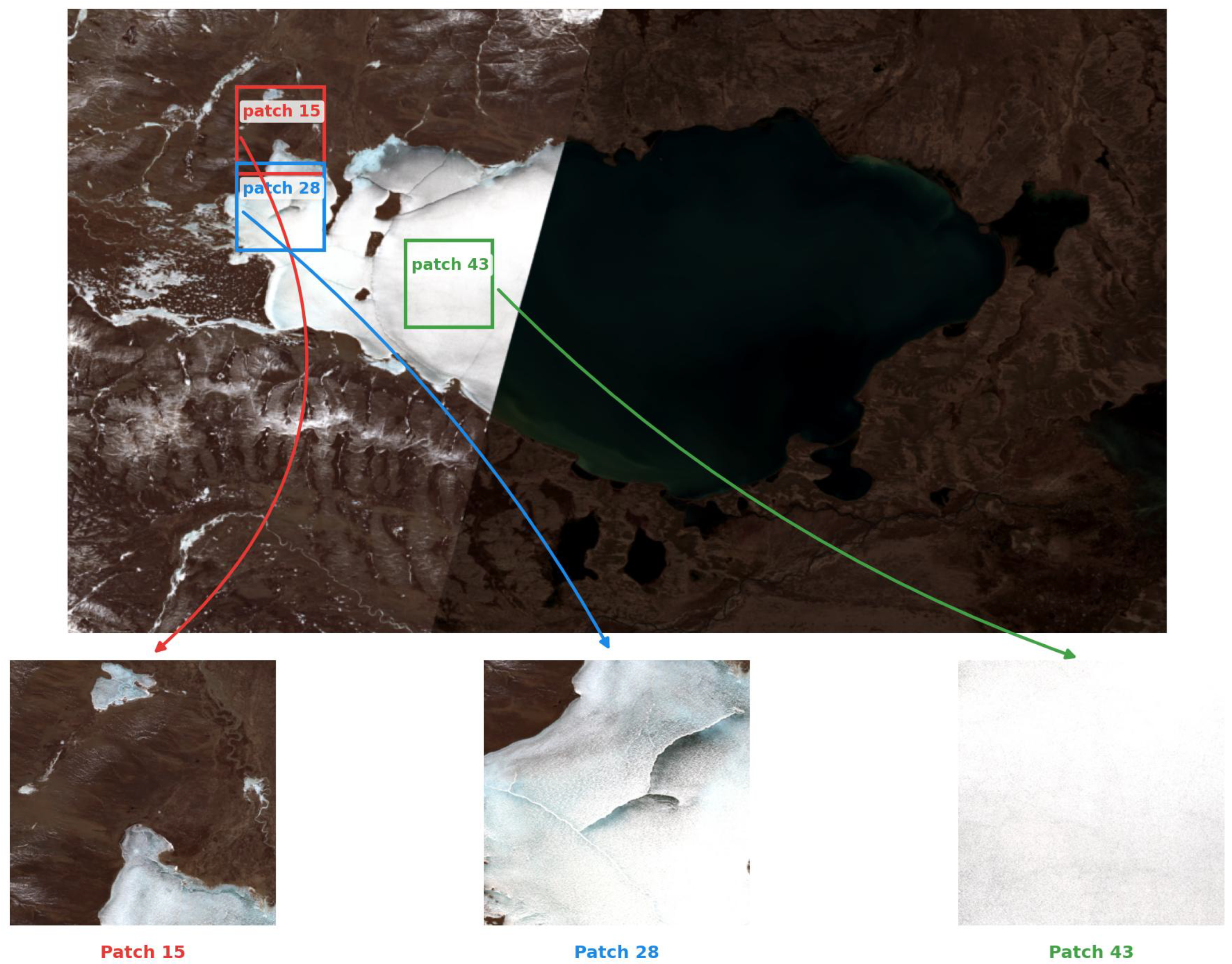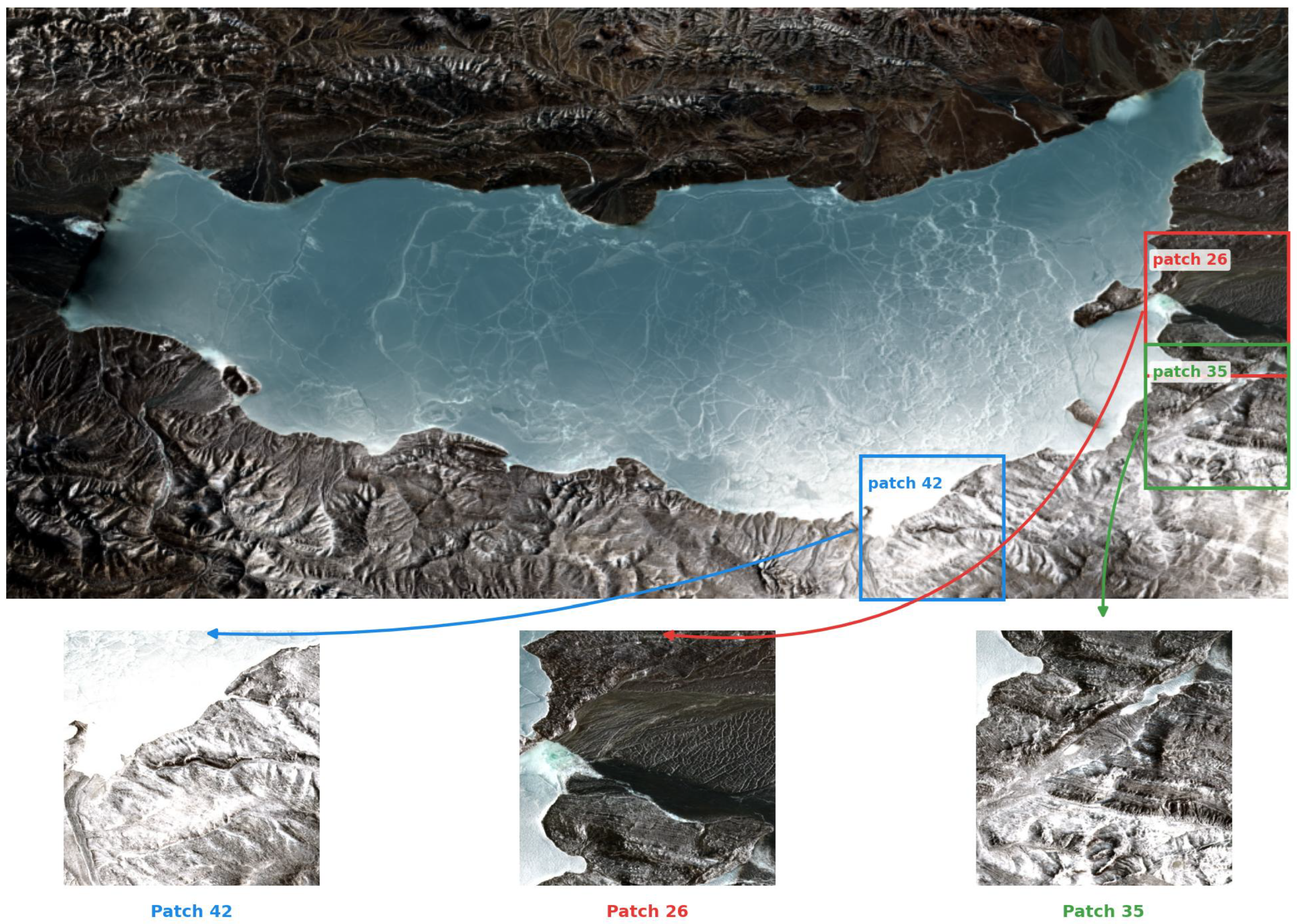As spatial resolution increases, a fixed-size image patch corresponds to a smaller ground area, reducing the spatial context available to the model [14]. In high-resolution remote sensing imagery, fixed-size local patches often contain insufficient semantic context for reliable lake recognition, particularly in regions affected by ice cover, shadows, or complex terrain backgrounds. Representative examples of local patch ambiguity are provided in Appendix A. Unlike common objects in conventional computer vision tasks, geographic targets in remote sensing imagery are often vast and spatially heterogeneous. Moreover, lake sizes on the Tibetan Plateau vary substantially, ranging from small fragmented ponds to extremely large inland lakes [7], further increasing the difficulty of achieving consistent segmentation performance across different spatial scales. In contrast, directly processing the entire high-resolution lake image requires substantial computational resources and usually necessitates image downsampling, which inevitably reduces boundary detail and weakens shoreline delineation accuracy [14,15]. As a result, high-resolution lake segmentation naturally requires simultaneously preserving large-scale semantic context and fine-scale shoreline geometry.

A wide range of methods have been proposed for lake extraction, from traditional spectral indices and object-based approaches to modern deep learning models [16,17,18,19,20]. While deep learning, particularly convolutional neural networks (CNNs) and Transformers, has shown significant progress [21,22], even advanced models still struggle with precise boundary delineation. Recent Transformer-based models can achieve very high region-overlap performance and IoU scores [23,24,25], yet stable shoreline localization remains challenging under complex alpine conditions [18,19,26]. Minor boundary deviations can lead to substantial errors in area estimation and downstream analyses, revealing a mismatch between region-level optimization and the need for geometric precision. An important factor contributing to this limitation is the widespread use of patch-based segmentation strategies, where image patches are processed independently [14,27,28]. Although computationally efficient, this approach restricts the model’s access to global spatial context, making it difficult to differentiate lakes from their surroundings. For large lakes, many local patches may contain only homogeneous water interiors without informative boundary cues, and independent patch processing discards information about the relative scale and spatial arrangement of the lake.

These observations suggest that approaches relying solely on either global context or local information are insufficient. In practice, human interpreters typically delineate lake boundaries from optical imagery by first understanding the overall lake structure and surrounding environment and then progressively examining local shoreline details at higher spatial scales. This implies that reliable shoreline delineation depends heavily on the integration of large-scale semantic context and fine-scale boundary information. Recent work in computer vision has shown that global–local and coarse-to-fine strategies are effective for improving boundary localization in complex tasks [29,30,31]. Similar paradigms have been explored in remote sensing for ultra-high-resolution imagery [32,33]. By combining global semantic understanding with local high-resolution refinement, these approaches can enhance geometric precision while maintaining structural consistency. Representative methods including RefineNet [34], OCRNet [35], GSCNN [30], and BASNet [31] have demonstrated the value of multi-scale feature aggregation and explicit boundary supervision. However, many existing approaches operate on fixed-resolution images and primarily improve segmentation quality through feature-level refinement within a single segmentation framework [31,34,35].

Despite these advances, such paradigms have not been fully explored for lake extraction in high-altitude environments. To address this gap, this study proposes a Global–Local Residual Refinement Network (GLR-Net), which explicitly integrates global contextual modeling with local patch-level refinement to achieve accurate lake boundary delineation. The main contributions of this study are as follows:

1.

We propose a global–local residual refinement framework that combines large-scale context modeling with patch-level boundary refinement to improve geometric shoreline accuracy.

2.

We design a boundary-oriented learning strategy that prioritizes local boundary correction under global structural guidance, enabling precise shoreline refinement while maintaining reliable lake extent recognition.

3.

Through comprehensive experiments on a Tibetan Plateau lake dataset, we demonstrate that the proposed method achieves consistent improvements in boundary accuracy compared to representative CNN and Transformer-based models.

4.

Our study reveals the trade-off between region-overlap metrics and geometric boundary precision, highlighting the importance of boundary-aware evaluation for practical lake delineation tasks.

2. Study Area and Data

2.1. Study Area

The study area is located on the Tibetan Plateau (approximately ${26}^{\circ }$–${40}^{\circ }$N, ${73}^{\circ }$–${105}^{\circ }$E), which is characterized by high elevation (generally above 4000 m), complex terrain, strong solar radiation, and harsh climatic conditions. The region contains a large number of high-altitude lakes that are highly sensitive to climate variability. In this region, lakes frequently exhibit seasonal freezing or partial ice cover. Meanwhile, surrounding surfaces such as snow cover, bright bare land, saline flats, and mountain shadows often present spectral characteristics similar to water bodies. These factors significantly reduce spectral separability between lakes and background surfaces, thereby increasing the difficulty of accurate lake boundary delineation from optical remote sensing imagery.

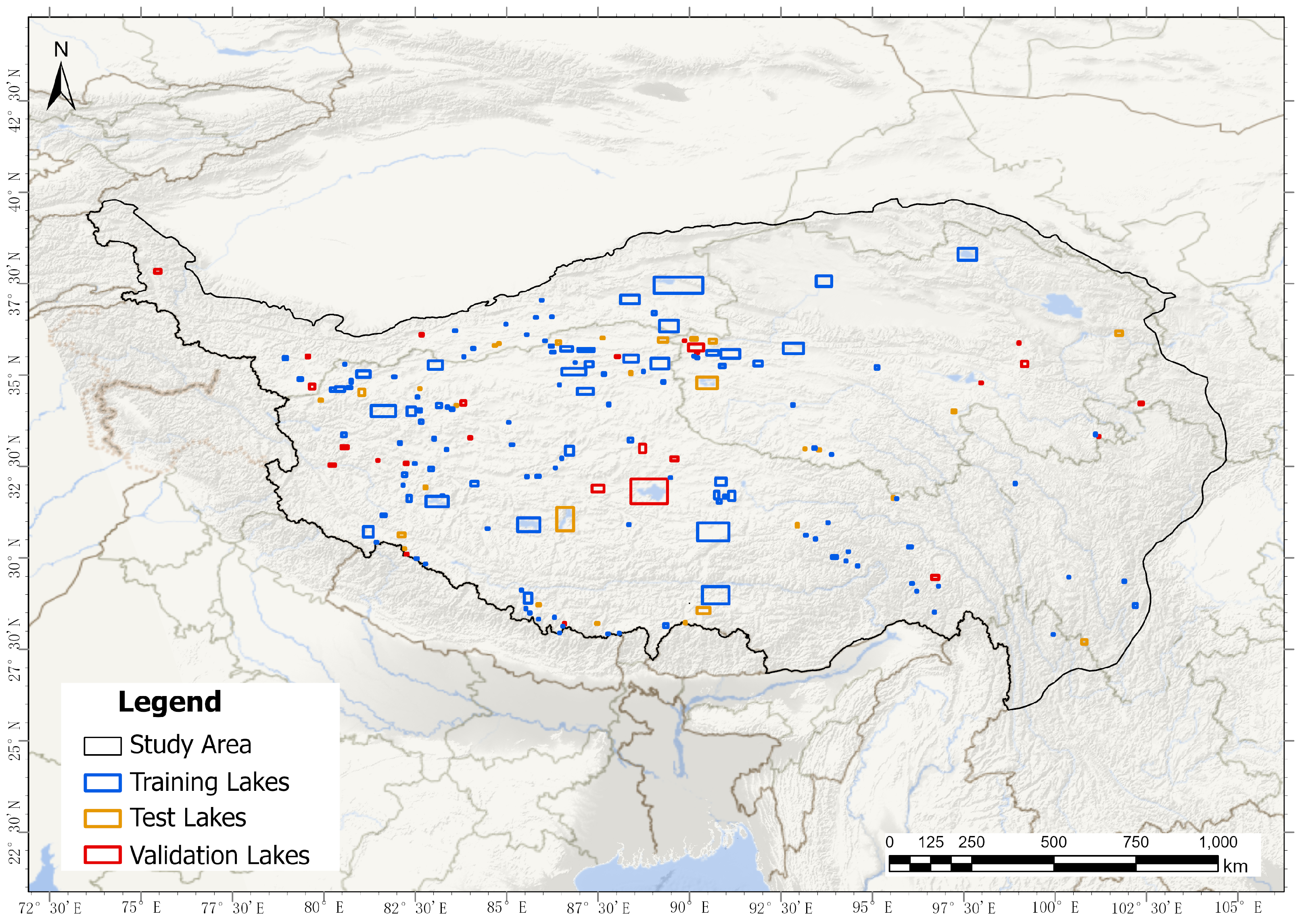
The Tibetan Plateau boundary adopted in this study was defined based on the official dataset released by the National Tibetan Plateau Data Center (TPDC). As shown in Figure 1, the collected lake samples are distributed across major lake-bearing regions of the plateau, covering diverse geomorphological and environmental conditions. This spatial diversity ensures that the dataset is representative of complex lake boundary characteristics under alpine environments.

2.2. Remote Sensing Data

Remote sensing imagery used in this study was acquired from the Google Earth Engine platform. The data source was the Sentinel-2 surface reflectance product COPERNICUS/S2_SR_HARMONIZED, which has undergone atmospheric correction and provides reliable surface spectral information suitable for lake boundary delineation.

Considering that optical imagery over the Tibetan Plateau is frequently affected by extensive cloud contamination during the summer season, Sentinel-2 imagery acquired from October 2024 to May 2025 was selected for dataset construction. This temporal range not only reduces cloud interference but also covers a complete winter freeze–thaw cycle, including the peak period of lake freezing and partial ice cover. As a result, the dataset contains a wide range of challenging shoreline delineation scenarios involving lake ice, snow cover, fragmented shorelines, mountain shadows, and spectrally ambiguous backgrounds under complex alpine environmental conditions. Four Sentinel-2 bands were used to construct the model input, including B4 (red), B3 (green), B2 (blue), and B8 (near-infrared). Among them, B2–B4 provide visible-spectrum information for characterizing the color and texture of lakes and surrounding land surfaces, while B8 is particularly effective for water-body discrimination and enhances contrast between lakes and non-water backgrounds.

For each lake sample, a 1000 m buffer was first generated around the lake boundary to ensure sufficient contextual information around lake boundaries while avoiding excessive background redundancy. Sentinel-2 images satisfying the temporal, spatial, and cloud-cover criteria were then collected within the buffered region and mosaicked by prioritizing pixels from images with lower cloud coverage. The final four-band lake sample image was obtained by clipping the mosaicked image to the buffered extent. This strategy minimizes cloud contamination while preserving complex spectral and spatial context around lake boundaries, thereby providing informative data for subsequent model learning.

2.3. Lake Boundary Dataset Construction

To construct a high-quality dataset for lake boundary delineation under complex alpine environments, a manually annotated Tibetan Plateau lake boundary dataset was established based on Sentinel-2 imagery. All lake boundaries were manually delineated lake by lake in ArcMap by experienced researchers using Sentinel-2 RGB and near-infrared composite imagery as interpretation references. The annotations were subsequently reviewed and corrected by another researcher to improve annotation consistency and geometric reliability. Because lake boundaries in alpine environments are frequently affected by ice cover, shadows, and bright surrounding backgrounds, automatic or semi-automatic labeling methods cannot guarantee sufficient boundary precision. Therefore, a fully manual fine-grained annotation strategy was adopted in this study.

For lakes with partial or complete ice cover, annotations were delineated according to the visually interpreted outer shoreline rather than the visible open-water extent. Samples with extremely ambiguous boundaries or severe cloud contamination were excluded during dataset construction whenever reliable visual interpretation was not possible.

A total of 179 lake samples were constructed, covering representative Tibetan Plateau lakes with diverse geographic locations, area scales, and background environments. Among them, 125, 26, and 28 lakes were assigned to the training, validation, and test sets, respectively. All samples were randomly split at the lake level into training, validation, and test subsets, ensuring no spatial overlap between subsets. The spatial distribution of the samples is shown in Figure 1. In terms of lake size, the constructed dataset covers a broad range of lake scales. Specifically, lake areas range from 27.30–5769.32 km² in the training set, 32.39–7072.57 km² in the validation set, and 29.85–3084.25 km² in the test set. This multi-scale distribution of lakes with highly variable spatial scales helps improve the model’s generalization ability across lakes of different sizes. Detailed statistics of the dataset are summarized in

Table 1. Statistics of the Lake Boundary Dataset.

Dataset	Number of Lakes	Min Area (km2)	Max Area (km2)
Train	125	27.30	5769.32
Val	26	32.39	7072.57
Test	28	29.85	3084.25
Total	179	27.30	7072.57

.

3. Methodology

3.1. Overall Framework

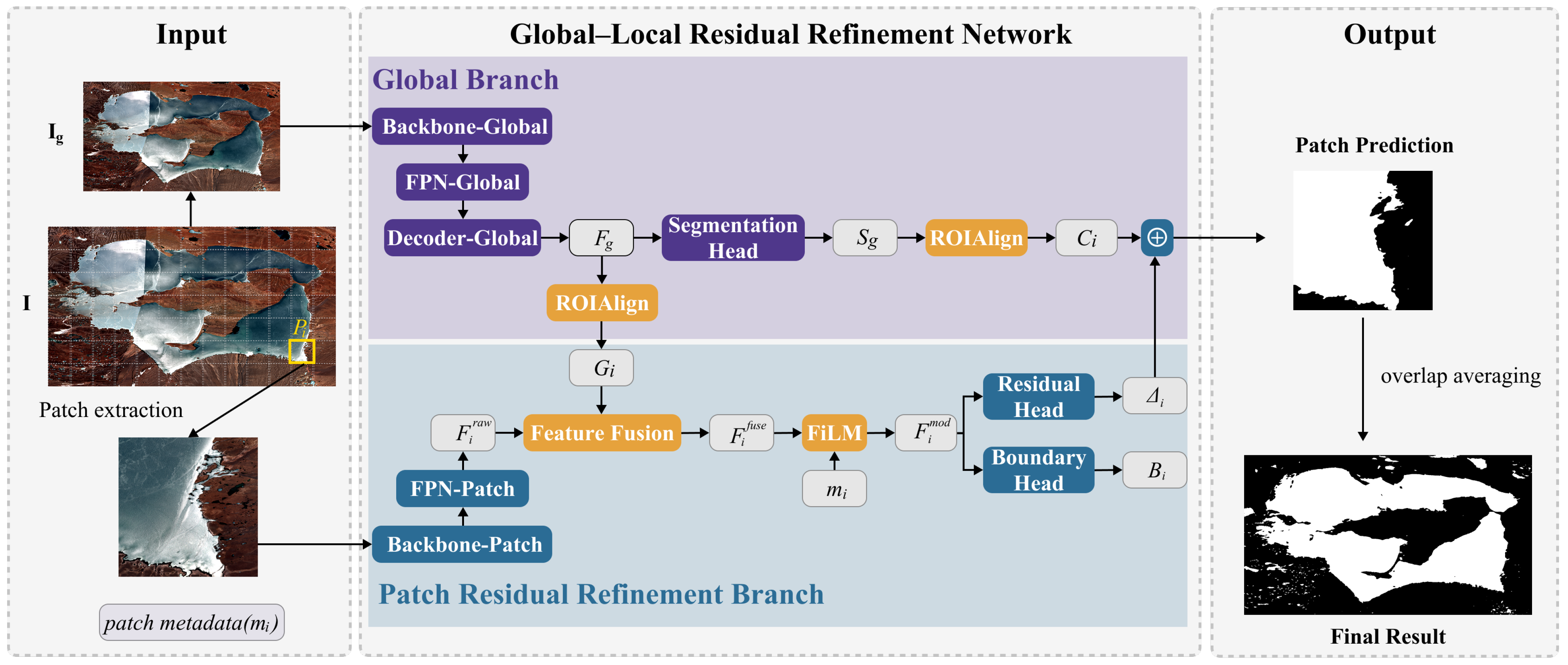
Figure 2 shows the workflow of the proposed GLR-Net, where a global branch provides coarse structural priors and a patch refinement branch refines local shoreline details through residual learning.

Let the input multispectral image be denoted as

$$\mathbf{I}\in {\mathbb{R}}^{H\times W\times C},$$

(1)

where $C=4$ and H and W denote the spatial dimensions. The framework consists of a Global Branch, a Patch Residual Refinement Branch, and a Global-to-Local Guidance Module.

The input image is first resized to obtain a global-scale image ${\mathit{I}}_g$. The global branch takes ${\mathit{I}}_g$ as input and produces the coarse segmentation prediction:

$${\mathit{S}}_g=f_g\left({\mathit{I}}_g\right).$$

(2)

where $f_g(·)$ denotes the mapping function of the global branch, which also outputs a fused decoder feature map ${\mathit{F}}_g$ used to provide semantic guidance for the subsequent local refinement branch.

The original-resolution image is then divided into local patches ${\left\{{\mathit{P}}_i\right\}}_{i=1}^N$. For each patch ${\mathit{P}}_i$, its spatial region is denoted as ${\mathit{ROI}}_i$. Based on ${\mathit{ROI}}_i$, the global outputs are cropped to obtain

$$\begin{array}{cc}\hfill {\mathit{C}}_i& =\mathit{Crop}({\mathit{S}}_g,{\mathit{ROI}}_i),\hfill \end{array}$$

(3)

$$\begin{array}{cc}\hfill {\mathit{G}}_i& =\mathit{Crop}({\mathit{F}}_g,{\mathit{ROI}}_i),\hfill \end{array}$$

(4)

where ${\mathit{C}}_i$ represents the local coarse segmentation prior and ${\mathit{G}}_i$ denotes the local semantic guidance feature. ${\mathit{S}}_g$ and ${\mathit{F}}_g$ denote the global prediction logits and decoder feature, respectively (see Section 3.2). ${\mathit{ROI}}_i$ defines the rectangular bounding box corresponding to the spatial region of the local patch.

Each patch is further associated with a spatial metadata vector ${\mathit{m}}_i$ encoding its normalized position and scale. The local branch takes $({\mathit{P}}_i,{\mathit{C}}_i,{\mathit{G}}_i,{\mathit{m}}_i)$ as input and predicts a residual correction ${\Delta }_i$ and a boundary response ${\mathit{B}}_i$. The refined prediction for each patch is obtained as

$${\widehat{\mathit{Y}}}_i={\mathit{C}}_i+{\Delta }_i.$$

(5)

Finally, all patch predictions are mapped back to the original spatial positions and aggregated to obtain the whole-lake segmentation result:

$$\widehat{\mathit{Y}}=\mathcal{A}\left({\left\{{\widehat{\mathit{Y}}}_i\right\}}_{i=1}^N\right),$$

(6)

where $\mathcal{A}(·)$ denotes overlap-aware spatial averaging. Overall, the global branch provides structural priors for lake recognition, while the local branch focuses on refining local shoreline details through residual correction.

3.2. Global Branch

Due to the high spatial resolution of remote sensing imagery, direct whole-image processing is computationally expensive and limits effective receptive field coverage. The global branch adopts an encoder–decoder architecture, where a ResNet-50 backbone is employed as the encoder to extract multi-scale features. Let the encoder outputs be denoted as $\{{\mathbf{E}}_1,{\mathbf{E}}_2,{\mathbf{E}}_3,{\mathbf{E}}_4\}$, corresponding to hierarchical feature maps at different scales. Their spatial resolutions are approximately ${\displaystyle \frac{1}{4}}$, ${\displaystyle \frac{1}{8}}$, ${\displaystyle \frac{1}{16}}$, and ${\displaystyle \frac{1}{16}}$ of the input image, respectively, where the final stage maintains a relatively high spatial resolution through dilated convolution.

To fuse semantic information across different scales, a Feature Pyramid Network (FPN) is introduced after the encoder to generate multi-scale feature representations with unified channel dimensions:

$$\{{\mathit{P}}_1,{\mathit{P}}_2,{\mathit{P}}_3,{\mathit{P}}_4\}=f_{\mathrm{fpn}}\left(\{{\mathbf{E}}_1,{\mathbf{E}}_2,{\mathbf{E}}_3,{\mathbf{E}}_4\}\right),$$

(7)

where $f_{\mathrm{fpn}}(·)$ denotes the top-down multi-scale feature fusion process.

Furthermore, a global context enhancement module is applied to the high-level features to model large-scale semantic dependencies, thereby improving the model’s perception of large-scale lake structures. The enhanced multi-scale features are then progressively fused by the decoder to obtain the global segmentation feature map:

$${\mathit{F}}_g=f_{\mathrm{dec}}\left(\{{\mathit{P}}_1,{\mathit{P}}_2,{\mathit{P}}_3,{\mathit{P}}_4\}\right),$$

(8)

where $f_{\mathrm{dec}}(·)$ denotes the multi-scale feature fusion and upsampling process.

Subsequently, the fused feature map is projected into segmentation logits through a classification head:

$${\mathit{S}}_g=f_{\mathrm{cls}}\left({\mathit{F}}_g\right),$$

(9)

where $f_{\mathrm{cls}}(·)$ denotes the classification mapping function implemented by a $1\times 1$ convolution.

The global branch produces two outputs: the coarse segmentation prediction ${\mathit{S}}_g$ and the fused decoder feature map ${\mathit{F}}_g$. Specifically, ${\mathit{S}}_g$ serves as the structural prior for lake segmentation, while ${\mathit{F}}_g$ provides semantic guidance for the local refinement branch. The global branch focuses on learning stable large-scale lake structures rather than precise boundary details, providing reliable priors for subsequent local refinement.

3.3. Global-to-Local Guidance Module

To fully exploit the structural information and semantic context provided by the global branch during local refinement, a Global-to-Local Guidance Module is designed to inject global information into the local branch through three mechanisms: feature cropping, semantic feature fusion, and FiLM-based spatial modulation. For each local patch ${\mathit{P}}_i$, the corresponding coarse segmentation prior ${\mathit{C}}_i$ and semantic feature ${\mathit{G}}_i$ are obtained by cropping the global outputs as defined in Equations (3) and (4).

The local branch first extracts raw patch-level features from the input patch:

$${\mathit{F}}_i^{\mathrm{raw}}=f_{\mathrm{patch}}\left({\mathit{P}}_i\right),$$

(10)

where $f_{\mathrm{patch}}(·)$ denotes the patch feature extractor of the local branch. Subsequently, the cropped global semantic feature ${\mathit{G}}_i$ is projected and fused with the raw patch feature to obtain the fused representation:

$${\mathit{F}}_i^{\mathrm{fuse}}=\varphi \left({\mathit{F}}_i^{\mathrm{raw}},{\mathit{G}}_i\right),$$

(11)

where $\varphi (·)$ represents concatenation followed by convolution-based fusion.

To further incorporate explicit spatial information, an eight-dimensional positional encoding vector is constructed for each local patch:

$${\mathit{m}}_i=\left(x_i,y_i,x_i^{\left(2\right)},y_i^{\left(2\right)},c_{x,i},c_{y,i},w_i,h_i\right),$$

(12)

where $x_i$ and $y_i$ denote the top-left corner coordinates of the patch, $x_i^{\left(2\right)}$ and $y_i^{\left(2\right)}$ denote the bottom-right corner coordinates, $c_{x,i}$ and $c_{y,i}$ denote the center coordinates, and $w_i$ and $h_i$ represent the width and height of the patch, respectively. A lightweight 8-dimensional positional encoding was adopted to provide spatial priors while keeping the modulation module compact under limited-data conditions. All positional features were normalized to the whole-image coordinate range before modulation.

The FiLM module generates feature-wise scaling and shifting parameters conditioned on both the cropped global semantic feature and the positional encoding vector:

$$({\gamma }_i,{\beta }_i)=f_{\mathrm{film}}({\mathit{G}}_i,{\mathit{m}}_i),$$

(13)

where ${\gamma }_i$ and ${\beta }_i$ denote the feature-wise scaling and shifting coefficients, respectively, and $f_{\mathrm{film}}(·)$ denotes the FiLM parameter generation function. The FiLM-based modulation mechanism enables the local refinement branch to adaptively refine shoreline structures according to both global semantic context and relative spatial location within the whole-lake structure.

The fused feature is then adaptively modulated through feature-wise affine transformation:

$${\mathit{F}}_i^{\mathrm{mod}}=(1+{\gamma }_i)\odot {\mathit{F}}_i^{\mathrm{fuse}}+{\beta }_i,$$

(14)

where ⊙ denotes element-wise multiplication. This modulation enables adaptive local feature refinement conditioned on both global semantic context and spatial location priors, improving global consistency and local discriminability.

3.4. Patch Residual Refinement Branch

The objective of the patch residual refinement branch is to perform fine-grained lake boundary segmentation at the original image resolution, thereby compensating for the boundary detail loss caused by downsampling in the global branch. Unlike conventional segmentation networks that directly predict complete segmentation masks, the proposed method adopts a residual refinement strategy, in which the local branch learns only the local correction relative to the coarse global prediction.

For each local patch ${\mathit{P}}_i$, the local branch first extracts local features from the image patch, which are subsequently guided by the global semantic feature ${\mathit{G}}_i$, coarse prior ${\mathit{C}}_i$, and positional metadata ${\mathit{m}}_i$ through the proposed global-to-local guidance mechanism. Multi-scale local features are extracted through an encoder–decoder architecture and transformed into the modulated feature representation ${\mathit{F}}_i^{\mathrm{mod}}$. Based on this feature, the model produces two prediction heads: a residual correction term ${\Delta }_i$ and a boundary response map ${\mathit{B}}_i$, formulated as

$$\begin{array}{cc}\hfill {\Delta }_i& =f_r\left({\mathit{F}}_i^{\mathrm{mod}}\right),\hfill \end{array}$$

(15)

$$\begin{array}{cc}\hfill {\mathit{B}}_i& =f_b\left({\mathit{F}}_i^{\mathrm{mod}}\right),\hfill \end{array}$$

(16)

where $f_r(·)$ denotes the residual prediction function and $f_b(·)$ denotes the boundary prediction function. The residual correction term is used to compensate for local errors in the coarse global prediction, while the boundary response map is employed during training to enhance the model’s attention to boundary regions.

The final prediction for each local patch is obtained by element-wise addition of the coarse prior and the predicted residual:

$${\widehat{\mathit{Y}}}_i={\mathit{C}}_i+{\Delta }_i.$$

(17)

In this manner, the local branch is not required to predict the complete segmentation result from scratch, but instead learns only the local discrepancy between the coarse global prediction and the ground truth, allowing the model to focus more effectively on correcting boundary and ambiguous regions.

Residual learning helps reduce optimization difficulty and improves training stability. After all local patches are processed, their predictions are mapped back to the original spatial positions and aggregated via overlap-aware averaging to improve spatial consistency across neighboring patches.

3.5. Loss Function

3.5.1. Loss in Stage 1

In the first stage, only the global branch is optimized, with the objective of learning stable whole-lake structural predictions. To this end, the stage-1 loss is defined as a combination of Dice loss and Top-k binary cross-entropy loss:

$${\mathcal{L}}_{\mathrm{stage}1}={\mathcal{L}}_{\mathrm{Dice}}+{\lambda }_{\mathrm{topk}}{\mathcal{L}}_{\mathrm{TopkBCE}},$$

(18)

where ${\lambda }_{\mathrm{topk}}$ denotes the weighting coefficient of the Top-k BCE loss, set to 0.3 in this study.

The Dice loss is formulated as

$${\mathcal{L}}_{\mathrm{Dice}}=1-{\displaystyle \frac{2{\sum }_n{p}_n{y}_n+ϵ}{{\sum }_n{p}_n+{\sum }_n{y}_n+ϵ}},$$

(19)

where $p_n$ and $y_n$ denote the predicted probability and ground-truth label of the n-th pixel, respectively, and $ϵ$ is a smoothing term to avoid division by zero. Dice loss measures the overlap between prediction and ground truth, thereby enforcing structural consistency at the region level.

The Top-k BCE loss focuses only on the hardest K pixels with the largest prediction errors:

$${\mathcal{L}}_{\mathrm{TopkBCE}}={\displaystyle \frac{1}{K}}\sum _{n\in {\mathrm{\Omega }}_K}{\mathcal{\ell }}_{\mathrm{BCE}}(p_n,y_n),$$

(20)

where ${\mathcal{\ell }}_{\mathrm{BCE}}(·)$ denotes the pixel-wise binary cross-entropy loss, ${\mathrm{\Omega }}_K$ denotes the set of the top K hardest pixels ranked by loss value, and K is determined by a predefined hard-sample ratio. In this study, the hard-sample ratio was set to 0.15. This strategy encourages the model to focus on difficult regions such as lake boundaries and snow/ice-confused areas, preventing training from being dominated by easy pixels.

3.5.2. Loss in Stage 2

In the second stage, the global branch is frozen and only the local refinement branch is optimized. Since this stage aims to model fine-grained lake boundary details, multiple loss terms are jointly employed for optimization:

$${\mathcal{L}}_{\mathrm{stage}2}={\lambda }_{\mathrm{seg}}{\mathcal{L}}_{\mathrm{seg}}+{\lambda }_{\mathrm{bnd}}{\mathcal{L}}_{\mathrm{bnd}}+{\lambda }_{\mathrm{cons}}{\mathcal{L}}_{\mathrm{cons}}+{\lambda }_{\mathrm{res}}{\mathcal{L}}_{\mathrm{res}},$$

(21)

where ${\mathcal{L}}_{\mathrm{seg}}$, ${\mathcal{L}}_{\mathrm{bnd}}$, ${\mathcal{L}}_{\mathrm{cons}}$, and ${\mathcal{L}}_{\mathrm{res}}$ denote the segmentation loss, boundary supervision loss, consistency constraint loss, and residual regularization loss, respectively. In this study, ${\lambda }_{\mathrm{seg}}$, ${\lambda }_{\mathrm{bnd}}$, ${\lambda }_{\mathrm{cons}}$, and ${\lambda }_{\mathrm{res}}$ were set to 1.0, 0.3, 0.3, and 0.1, respectively. In addition, ${\lambda }_{\mathrm{wbce}}$ was set to 0.3.

The segmentation loss is defined as

$${\mathcal{L}}_{\mathrm{seg}}={\mathcal{L}}_{\mathrm{Dice}}^p+{\lambda }_{\mathrm{wbce}}{\mathcal{L}}_{\mathrm{WBCE}},$$

(22)

where ${\mathcal{L}}_{\mathrm{Dice}}^p$ denotes the patch-level Dice loss, ${\mathcal{L}}_{\mathrm{WBCE}}$ denotes the weighted binary cross-entropy loss, and ${\lambda }_{\mathrm{wbce}}$ is its weighting coefficient. The weight map of the weighted BCE loss is generated from the ground-truth boundary regions to enhance the model’s attention to boundary areas.

To further strengthen boundary learning, a boundary supervision loss is introduced:

$${\mathcal{L}}_{\mathrm{bnd}}={\mathcal{\ell }}_{\mathrm{BCE}}({\mathit{B}}_i,{\mathit{B}}_i^{*}),$$

(23)

where ${\mathit{B}}_i^{*}$ denotes the ground-truth shoreline boundary mask generated by rasterizing the manually delineated shoreline vectors with spatial alignment to the corresponding image grid in ArcMap.

To maintain consistency between local predictions and the global structural prior, a consistency constraint term is introduced:

$${\mathcal{L}}_{\mathrm{cons}}={∥\sigma \left({\widehat{\mathit{Y}}}_i\right)-\sigma \left({\mathit{C}}_i\right)∥}_1,$$

(24)

where $\sigma (·)$ denotes the Sigmoid activation function. This term constrains the refined local prediction from deviating excessively from the coarse global prediction in probability space, thereby preserving consistency with the global structural prior. The L1 formulation was adopted because it provides stable probability-space regularization while avoiding overly strong penalization of local refinement corrections.

In addition, to prevent the model from producing excessively large local corrections, a residual regularization term is introduced:

$${\mathcal{L}}_{\mathrm{res}}={∥{\Delta }_i∥}_1,$$

(25)

which constrains the magnitude of the residual correction, thereby improving training stability and suppressing over-correction.

4. Experiments

All experiments were implemented in PyTorch 2.5.1 (CUDA 12.1) and conducted using the same training, validation, and test split. All models, including the proposed method and baseline models, were trained and evaluated under identical data preprocessing and evaluation protocols to ensure a fair comparison. Each sample corresponds to one cropped whole-lake scene. The training, validation, and test sets are spatially independent, with no overlap in lake regions across the three subsets, ensuring that no spatial information leakage occurs during model training and evaluation.

The proposed framework was compared with representative CNN-based and Transformer-based semantic segmentation models under identical experimental settings. U-Net represents a classical convolution-based encoder–decoder architecture widely used in remote sensing image segmentation [21]. SegFormer is a transformer-based segmentation model with strong global context modeling capability and pretrained representations [22]. OCRNet is a representative context-aware segmentation model that enhances pixel representations through object-region contextual aggregation while preserving high-resolution spatial features [35].

4.1. Input Data and Preprocessing

Each lake sample consists of a four-channel remote sensing image and a corresponding binary water mask. Channel-wise mean and standard deviation were computed from the training set and used to normalize inputs during training, validation, and testing to ensure consistent preprocessing across all experiments. To reduce computational cost while preserving the overall lake geometry, each whole-lake image was resized while maintaining its original aspect ratio. The longer side was constrained to 1024 pixels. Bilinear interpolation was applied to the input images, whereas nearest-neighbor interpolation was used for the binary masks to avoid boundary distortion.

For the proposed method, the resized whole-lake image was first processed by a global branch to capture large-scale spatial context. In the second stage, the original-resolution lake image was partitioned into local patches of $512\times 512$ pixels for shoreline refinement. Patch starting coordinates were adaptively generated along each spatial dimension to ensure full spatial coverage of the entire lake region. When overlap occurred between adjacent patches, the overlapping predictions were averaged during reconstruction to produce the final full-resolution segmentation result.

During Stage-2 training, up to 24 patches were sampled per lake depending on lake size and the availability of valid sampling regions. Boundary-prioritized patches were sampled from regions with high boundary density in the ground-truth mask to emphasize shoreline learning, while the remaining patches were randomly sampled to maintain spatial diversity and improve generalization. In the final experiments, boundary-prioritized and random patches accounted for 40% and 60% of the sampled patches, respectively. All baseline models operated in a single-stage manner and used only the resized whole-lake image as input without local patch refinement.

4.2. Training Protocol

All models were trained with a batch size of 1 because each sample corresponds to one complete lake and lake sizes vary substantially. Mixed-precision training and gradient clipping were applied to improve optimization stability. The Adam optimizer was used for all experiments with an initial learning rate of $5\times {10}^{-5}$ and a weight decay of $5\times {10}^{-4}$. A ReduceLROnPlateau learning rate scheduler and an early stopping strategy were adopted to stabilize training and reduce overfitting.

The proposed framework was trained in a two-stage coarse-to-fine manner. In Stage 1, only the Global Branch was optimized to learn coarse lake localization and region-level semantic representations. The Global Branch employed a ResNet-50 backbone followed by an FPN and a decoder module. The optimization objective in Stage 1 consisted of Dice loss and Top-k binary cross-entropy loss, where the Top-k ratio was set to 0.15, meaning that only the top 15% highest-loss pixels within each training sample were used for binary cross-entropy optimization. The Top-k BCE term was weighted by 0.3. In Stage 2, the best checkpoint obtained from Stage 1 was loaded, and the parameters of the Global Branch were frozen. Only the Patch Residual Refinement Branch and the Global-to-Local Guidance Module were optimized. The optimization objective in Stage 2 consisted of a patch segmentation loss, a boundary prediction loss, a consistency loss, and a residual regularization term. The patch segmentation loss combined Dice loss with boundary-weighted binary cross-entropy loss to enhance shoreline refinement performance. Boundary pixels were assigned larger spatial weights during optimization. The consistency loss and residual regularization terms were weighted by ${\lambda }_{\mathrm{cons}}=0.3$ and ${\lambda }_{\mathrm{res}}=0.1$, respectively. These hyperparameters were empirically determined based on validation performance stability. The same optimizer settings and training protocols were applied to all baseline models whenever applicable.

4.3. Baseline Models

Three representative semantic segmentation models were selected for comparison: U-Net, SegFormer, and OCRNet [21,22,35]. For the transformer-based SegFormer architecture, both the lightweight SegFormer-B0 and the larger SegFormer-B4 variants were evaluated to investigate the influence of model capacity and pretrained semantic representations on shoreline delineation performance.

U-Net was implemented as a convolutional encoder–decoder baseline with four-channel input and bilinear upsampling in the decoder. SegFormer-B0 is a hierarchical transformer-based segmentation model. In this study, the SegFormer-B0 configuration with an MiT-B0 encoder was adopted. The model was initialized from the official SegFormer-B0 checkpoint pretrained on ADE20K. Since the original checkpoint was trained with three-channel RGB inputs, the first patch embedding layer was adapted to accept four-channel Sentinel-2 inputs by initializing the additional channel with the mean of the pretrained RGB-channel weights. The final segmentation classifier was randomly initialized because the ADE20K checkpoint was trained for 150-class semantic segmentation, whereas this study focuses on binary lake segmentation. SegFormer-B0 was selected as a representative lightweight transformer-based baseline because it provides a favorable balance between segmentation capability, training stability, and computational cost for the whole-lake segmentation setting adopted in this study. Larger transformer variants markedly increase memory consumption during high-resolution dense prediction and may reduce training stability under limited-data conditions. In addition, a larger SegFormer-B4 variant was further evaluated using the same training and evaluation protocol. The SegFormer-B4 model adopts a MiT-B4 encoder with considerably higher model capacity and stronger pretrained semantic representations compared with SegFormer-B0.

OCRNet is a representative context-aware semantic segmentation model that enhances pixel representations through object-region contextual aggregation. In this study, OCRNet was implemented based on the MMSegmentation framework using an HRNetV2p-W18 backbone. The backbone was initialized using the official ADE20K-pretrained checkpoint provided by MMSegmentation. The model was adapted to accept four-channel Sentinel-2 inputs and configured for binary lake segmentation. Specifically, the first convolutional layer was modified to process four-channel multispectral imagery, while the final classification layer was adjusted to output a single foreground class. OCRNet was selected because it combines high-resolution feature representations with object-level contextual reasoning, making it suitable for comparison with both convolution-based and transformer-based segmentation models under complex shoreline conditions. Although dedicated boundary-aware segmentation methods may provide additional comparison perspectives, the primary objective of this study was to evaluate whether the proposed global–local refinement framework can improve geometric shoreline accuracy relative to representative mainstream segmentation paradigms under identical training and evaluation settings.

To ensure a fair comparison, all baseline models were trained and evaluated using the same dataset split, normalization strategy, and whole-lake resizing protocol as the proposed method.

4.4. Evaluation Metrics

To comprehensively evaluate segmentation performance at both regional and boundary levels, several evaluation metrics were adopted, including Intersection over Union (IoU), Dice coefficient, Lake-level IoU, Boundary F1 score (BF1), and Boundary Distance Error (BDE).

IoU and Dice were used to evaluate the pixel-level overlap between predicted masks and ground-truth masks. Since lake sizes vary markedly across the dataset, Lake-level IoU was additionally computed by first calculating the IoU for each individual lake and then averaging the results across all lakes in the test set. This metric reduces the dominance of large lakes and provides a more balanced evaluation of segmentation performance at the lake scale.

Boundary-based metrics were further introduced to evaluate shoreline delineation accuracy. Boundary F1 score (BF1) measures the correspondence between predicted and ground-truth boundaries based on boundary precision and recall within a predefined tolerance radius. BF1 scores were first computed independently for each lake and then averaged across all lakes in the test set. In this study, a 3-pixel tolerance radius was adopted to account for minor spatial boundary misalignment between predicted and reference boundaries.

Boundary Distance Error (BDE) was used to quantify the spatial deviation between predicted and ground-truth shorelines. First, boundary pixels were extracted by subtracting a morphologically eroded mask from the original binary mask using a $3\times 3$ structuring element. Euclidean distance transforms were then used to compute the distance from each ground-truth boundary pixel to the nearest predicted boundary pixel and, conversely, from each predicted boundary pixel to the nearest ground-truth boundary pixel. The two sets of distances were combined to obtain a symmetric boundary distance distribution. Unlike BF1, which was averaged at the lake level, the BDE statistics were computed from globally aggregated bidirectional boundary-distance samples extracted from the complete test set. The mean, median, and 90th-percentile BDE values were then reported in pixels.

Compared with region-overlap metrics such as IoU and Dice, boundary-aware metrics provide a more direct evaluation of geometric shoreline accuracy, which is particularly important for lake inventory mapping and hydrological applications requiring reliable boundary delineation.

5. Results

5.1. Quantitative Comparison with Existing Methods

To evaluate the effectiveness of the proposed framework, its performance was compared with several representative semantic segmentation models, including U-Net, SegFormer-B0, SegFormer-B4, and OCRNet. The quantitative comparison results are summarized in

Table 2. Quantitative comparison of lake extraction performance on the test dataset.

Method	IoU	Dice	Lake-Level IoU	BF1 (3-Pixel Tolerance)	Mean BDE (px)
U-Net	0.915	0.956	0.787	0.712	23.99
SegFormer-B0	0.959	0.979	0.913	0.778	19.18
SegFormer-B4	0.966	0.983	0.930	0.804	17.47
OCRNet	0.961	0.980	0.915	0.783	16.46
Ours	0.944	0.971	0.872	0.811	13.19

. All models were trained and evaluated using the same training, validation, and test datasets under identical experimental settings to ensure a fair comparison.

Among the compared methods, the proposed approach achieves the highest Boundary F1 score (0.811) while consistently reducing boundary errors compared with U-Net, SegFormer-B0, SegFormer-B4, and OCRNet. These results suggest that the proposed global–local refinement framework can better preserve fine-scale shoreline geometry. While SegFormer-B0, SegFormer-B4, and OCRNet achieve strong performance in region-based metrics, including IoU, Dice, and lake-level IoU, these metrics primarily reflect region overlap rather than geometric shoreline accuracy.

These findings highlight the importance of explicit local boundary refinement and boundary-aware evaluation for reliable shoreline localization beyond conventional region-overlap optimization.

To account for uncertainty caused by the relatively limited number of test lakes, bootstrap 95% confidence intervals were computed for lake-level metrics using 10,000 resampling iterations. As shown in

Table 3. Bootstrap 95% confidence intervals for lake-level evaluation metrics on the test set (n = 28, B = 10,000).

Method	BF1 Mean	BF1 95% CI	Lake-Level IoU Mean	Lake-Level IoU 95% CI
U-Net	0.712	[0.619, 0.801]	0.787	[0.674, 0.890]
SegFormer-B0	0.778	[0.701, 0.849]	0.913	[0.858, 0.954]
SegFormer-B4	0.804	[0.731, 0.869]	0.930	[0.886, 0.959]
OCRNet	0.783	[0.709, 0.846]	0.915	[0.868, 0.950]
Ours	0.811	[0.736, 0.875]	0.872	[0.795, 0.933]

, the confidence intervals of several models overlap, indicating that small numerical differences in region-overlap metrics should be interpreted with caution. Nevertheless, the proposed method achieves the highest mean Boundary F1 score while maintaining competitive lake-level IoU, supporting its advantage in boundary-aware evaluation.

5.2. Qualitative Results

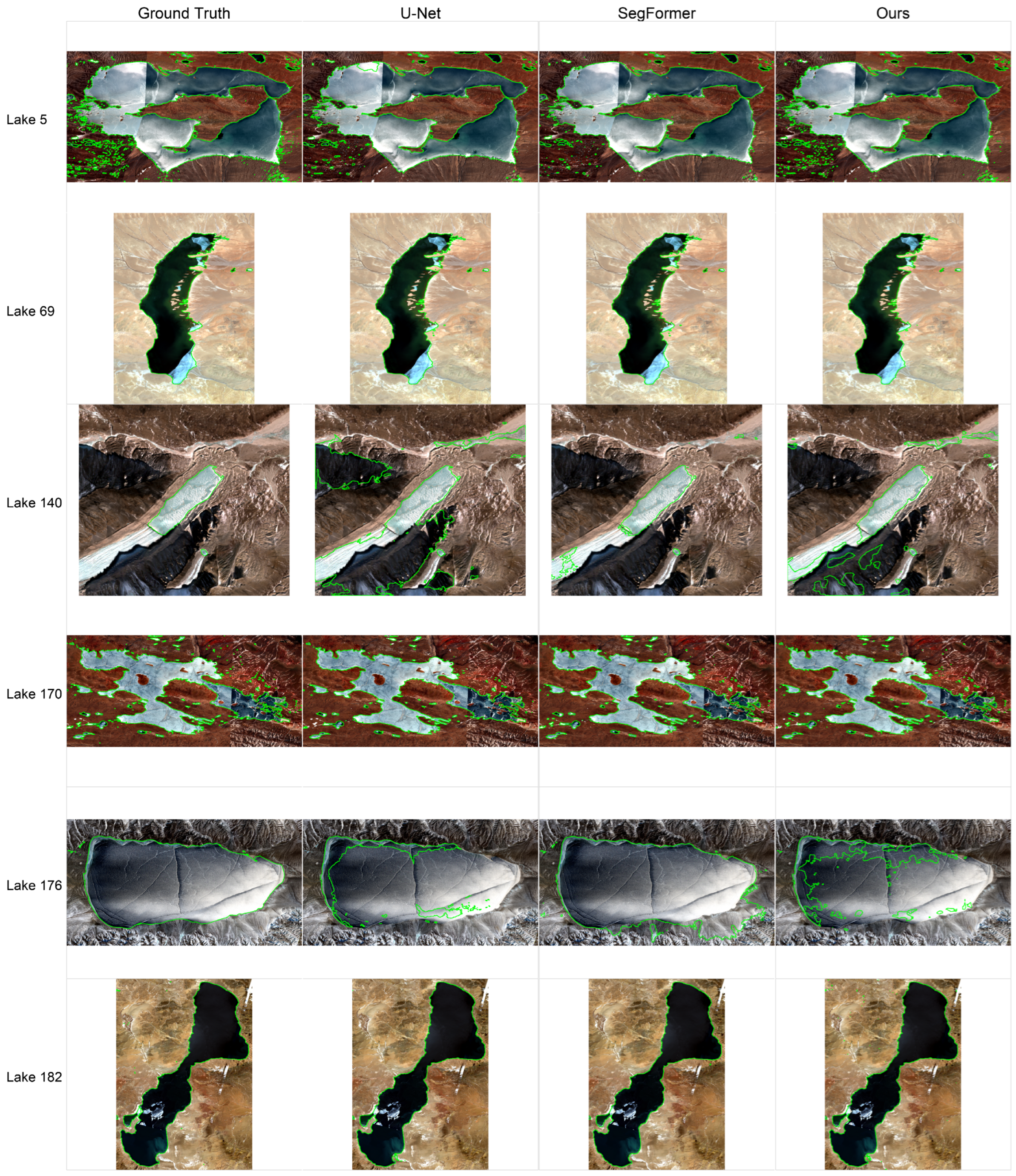
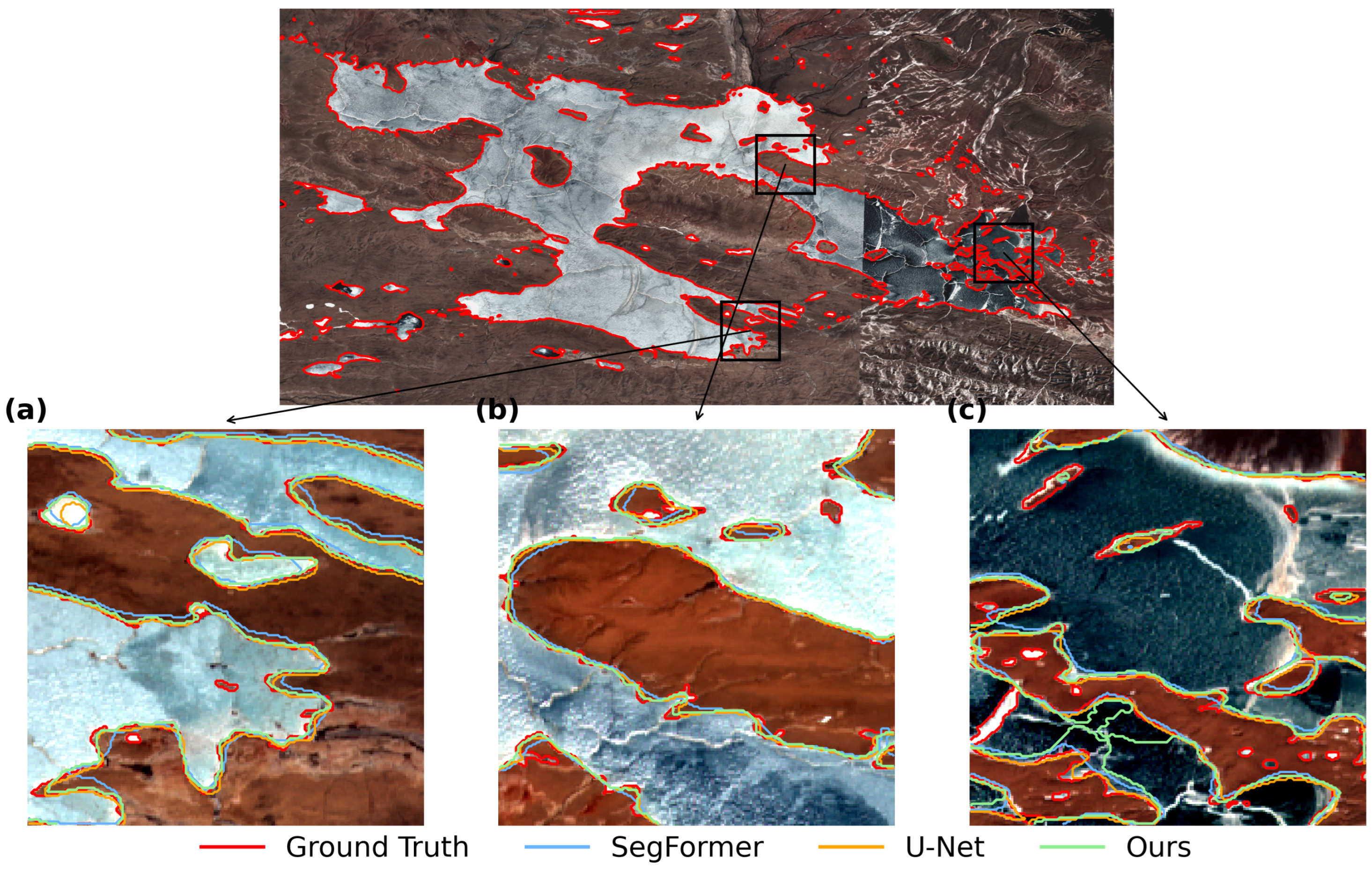
In addition to quantitative evaluation, visual comparisons were conducted to further analyze the performance of different models. Several representative lakes from the test dataset were selected to illustrate the segmentation results under different environmental conditions. Figure 3 presents qualitative comparisons of lake boundary extraction results produced by U-Net, SegFormer-B0, and the proposed method. Overall, most models are able to capture the general spatial extent of large lakes under relatively clear spectral conditions. In contrast, noticeable differences can be observed in complex scenarios, particularly for partially ice-covered lakes and fragmented water bodies.

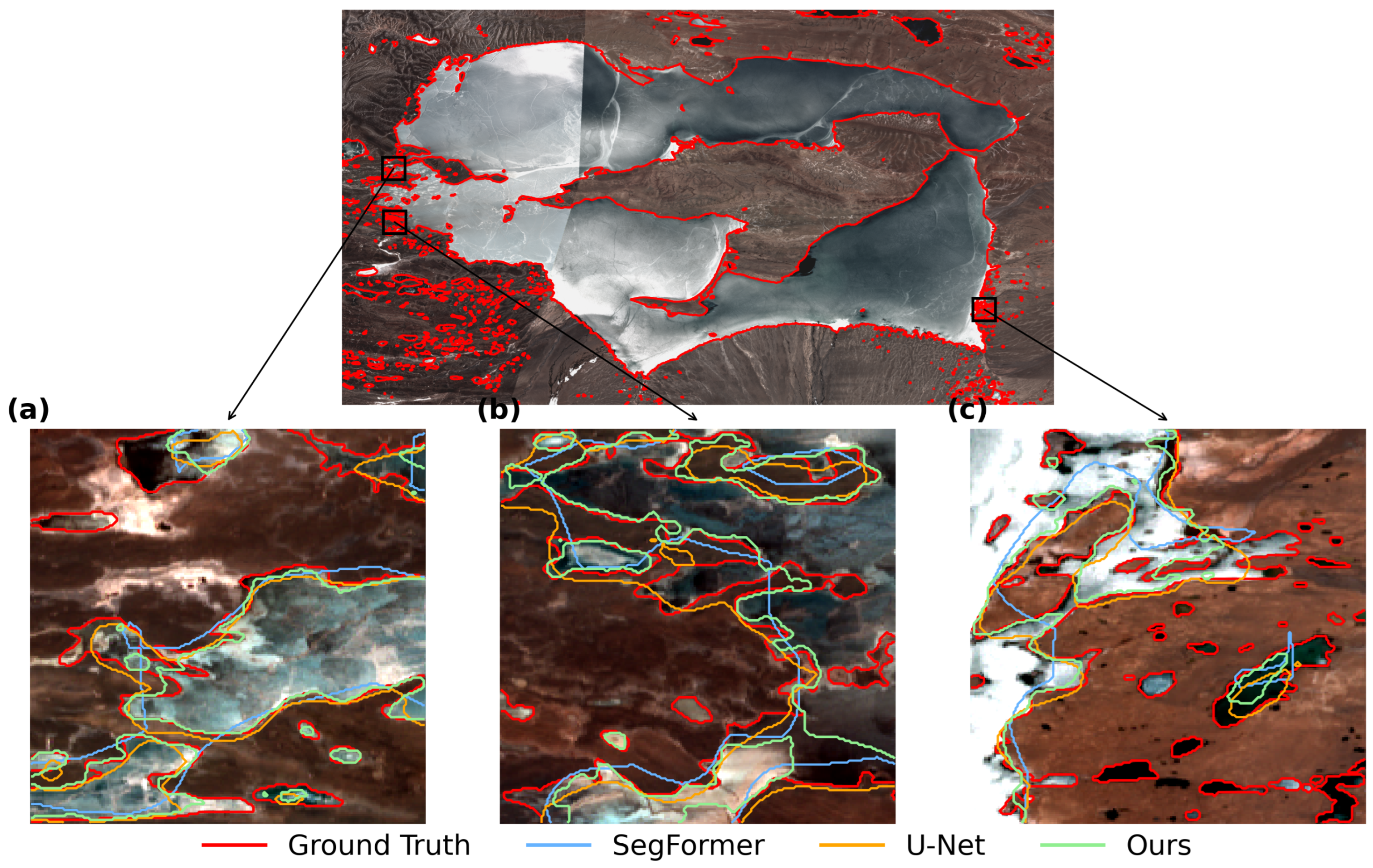
Specifically, although baseline models can achieve reasonable region-level segmentation, they often exhibit boundary irregularities, noise, and misclassification near shoreline regions. In contrast, the proposed method produces cleaner and more spatially consistent boundaries, demonstrating improved shoreline localization. For example, in Lake 5 and Lake 170, baseline models produce noticeable noise and misclassification in surrounding regions, whereas the proposed method generates cleaner and more consistent shoreline boundaries. Detailed boundary comparisons for these cases are shown in Figure 4 and Figure 5, respectively. These results indicate that the global–local refinement framework can effectively improve geometric shoreline delineation in complex environments. Importantly, these qualitative observations are consistent with the quantitative results, where models with comparable region-overlap metrics may still exhibit substantial differences in geometric boundary quality.

Failure cases are also observed. For instance, in Lake 176, which contains extensive ice cover, the model struggles to accurately recognize the complete lake extent under extreme spectral ambiguity. This observation further suggests that reliable shoreline delineation depends not only on local boundary refinement but also on robust large-scale semantic recognition under complex environmental conditions. OCRNet was excluded from the qualitative comparison figure to avoid excessive visual complexity. Quantitative evaluation results for OCRNet are provided in Table 2 and

Table 4. Statistical boundary error comparison of different methods.

Method	Mean BDE (px)	Median BDE (px)	P90 BDE (px)
U-Net	23.99	2.00	79.00
SegFormer-B0	19.18	2.24	30.41
SegFormer-B4	17.47	2.00	21.10
OCRNet	16.46	2.23	31.14
Ours	13.19	1.00	22.67

.

5.3. Boundary Error Analysis

To further analyze geometric shoreline delineation quality, boundary distance errors were computed for all models. The statistical results of boundary errors are summarized in Table 4. Specifically, bidirectional nearest-boundary distances between predicted and ground-truth boundaries were calculated using Euclidean distance transforms.

The proposed method achieves the lowest Mean BDE and Median BDE among all compared models. In particular, the mean BDE decreases to 13.19 pixels, compared with 19.18 pixels for SegFormer-B0, 17.47 pixels for SegFormer-B4, 16.46 pixels for OCRNet, and 23.99 pixels for U-Net. Although SegFormer-B4 achieves a slightly lower P90 BDE, the proposed framework consistently improves average shoreline localization accuracy while maintaining competitive robustness against large boundary deviations.

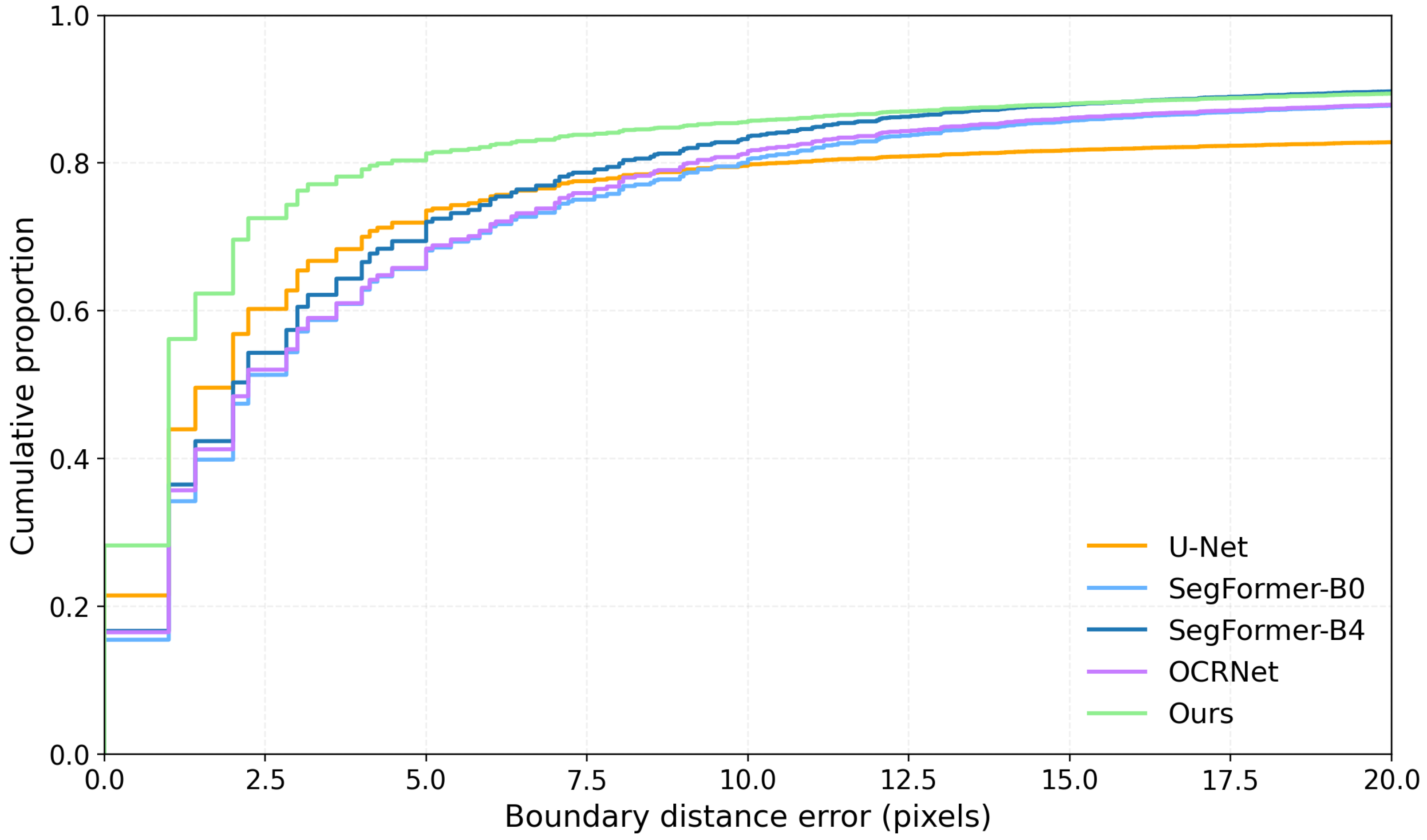
Figure 6 further illustrates the cumulative distribution of boundary distance errors across the test dataset. Compared with the baseline models, the proposed method exhibits a larger proportion of boundary samples with small localization errors, particularly in the low-error range, indicating improved geometric shoreline delineation capability under complex shoreline conditions.

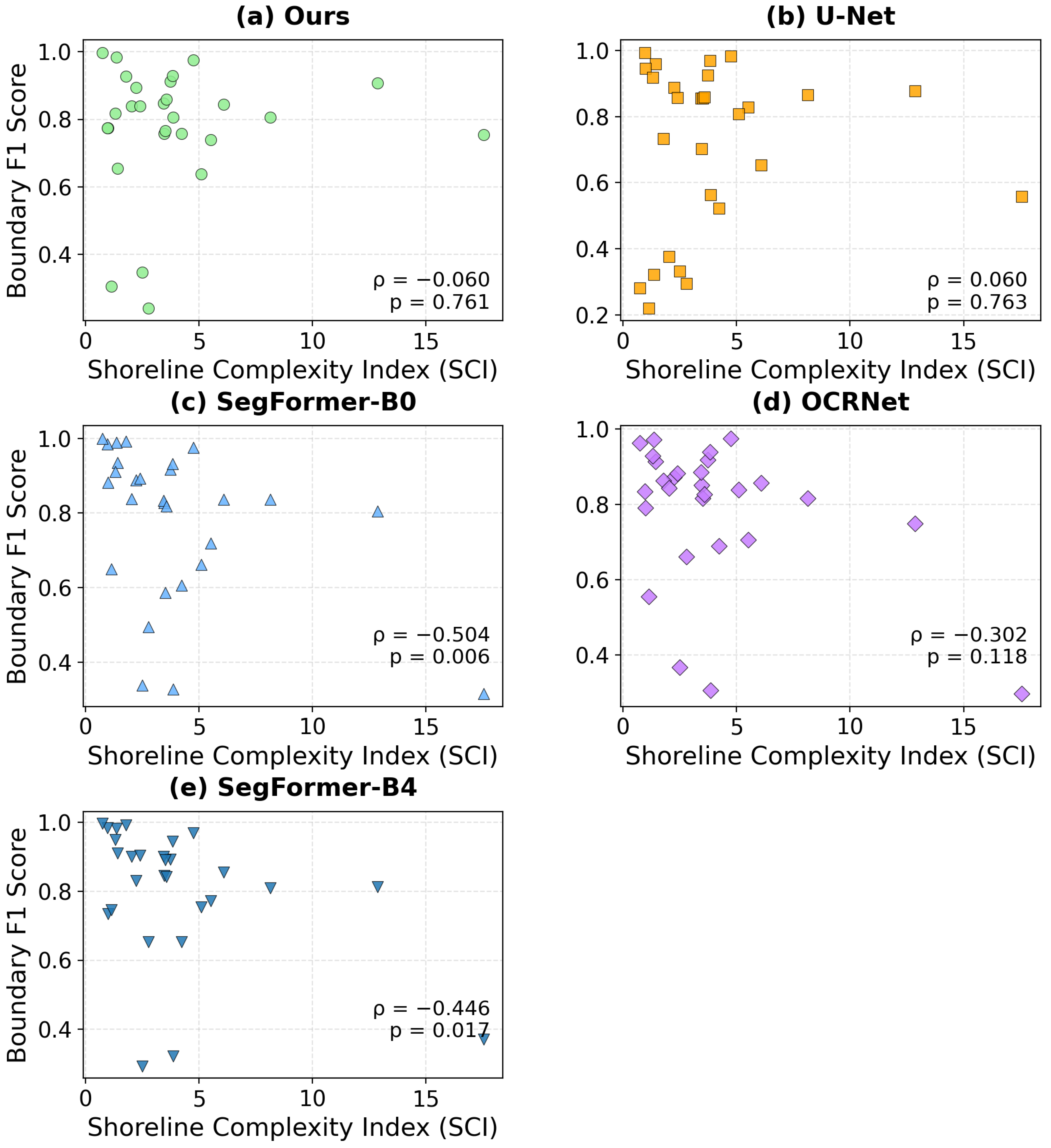
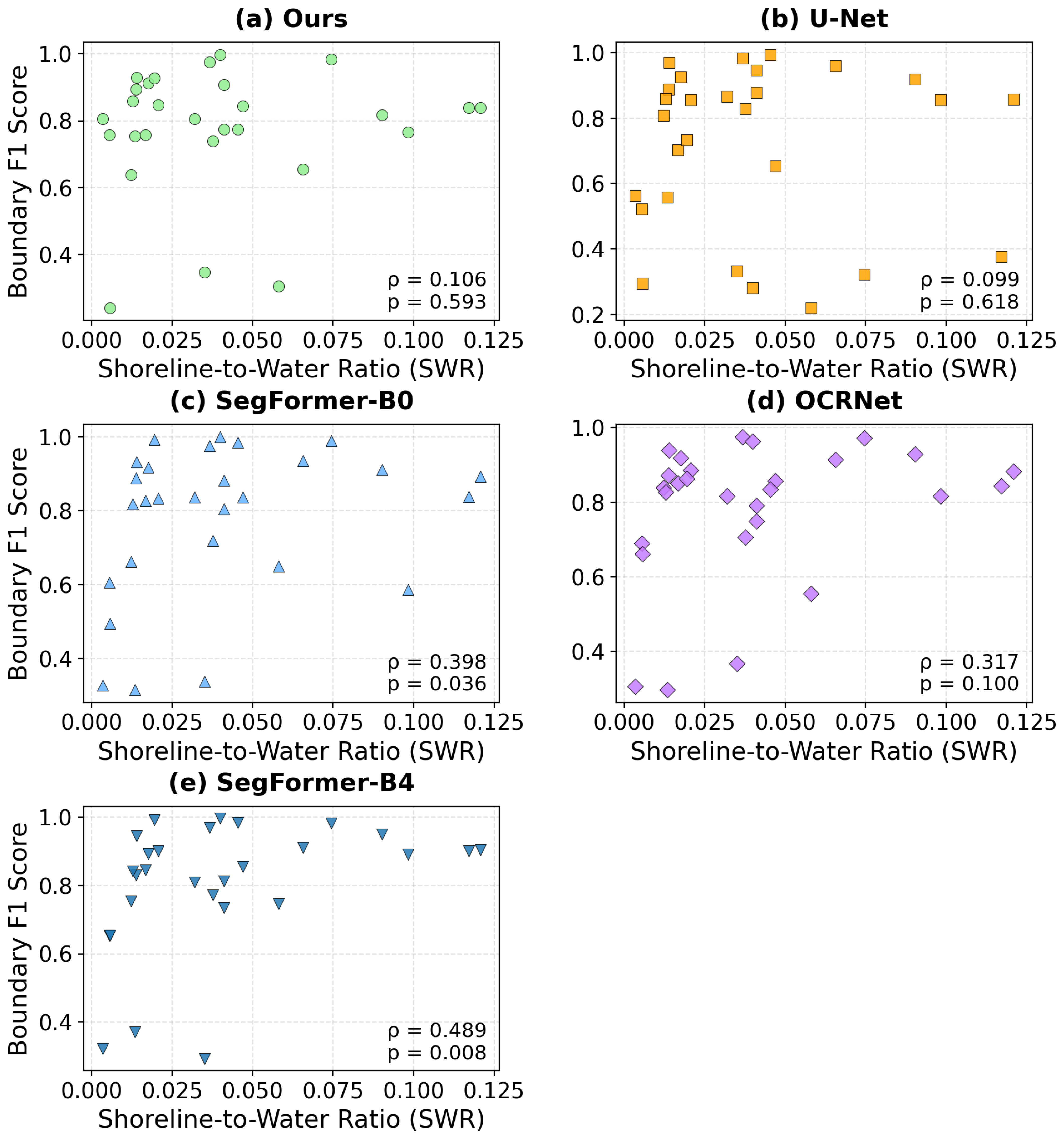
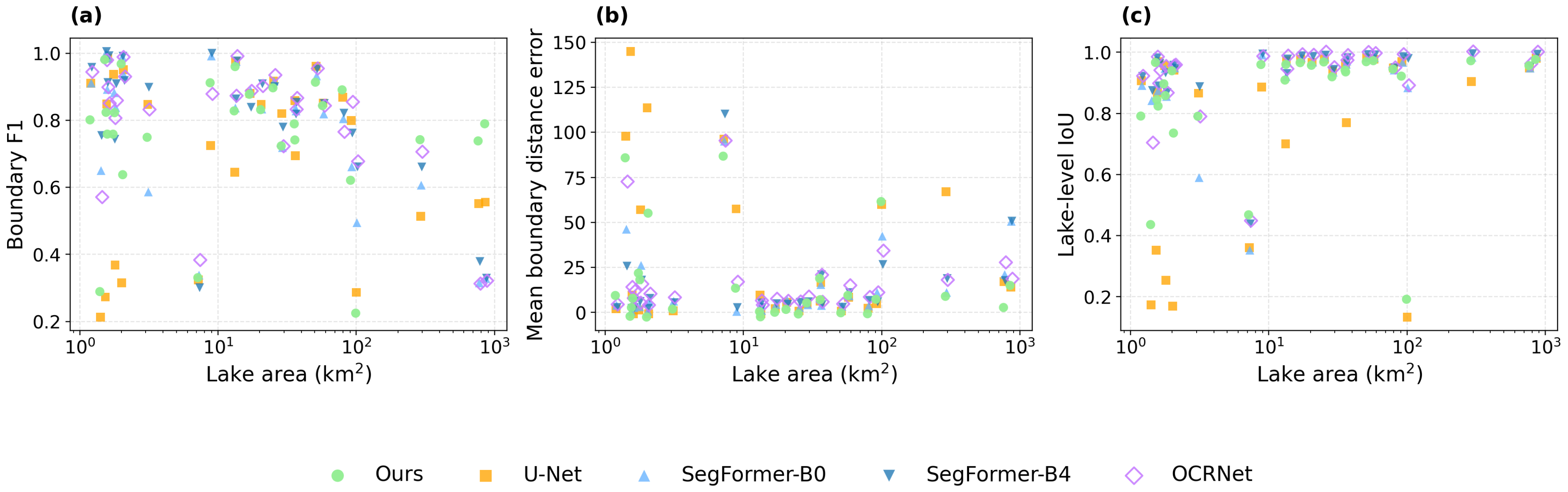
Importantly, these results reveal that models with similarly high region-overlap performance may still exhibit noticeably different geometric shoreline quality. This observation is consistent with the quantitative and qualitative analyses, highlighting that region-overlap metrics alone are insufficient for evaluating shoreline delineation quality. Per-lake statistics in Appendix B further demonstrate that high Boundary F1 scores do not necessarily correspond to low geometric boundary errors.

These observations further support the effectiveness of the proposed global–local framework in improving boundary fidelity through the integration of large-scale structural context and local boundary refinement.

5.4. Ablation Study

To evaluate the contribution of different components in the proposed framework, an ablation study was conducted using four model variants: a global-only model, a patch-only model, a model without global-to-local conditioning, and the full model. The global-only model corresponds to the global segmentation branch without the patch-level refinement stage, while the patch-only model removes the global structural guidance and directly performs local patch-based prediction. The variant without global-to-local conditioning retains the dual-branch architecture and residual refinement strategy but removes explicit global feature conditioning in the patch refinement branch.

Table 5. Ablation study evaluating the contributions of global semantic context, local refinement, and global-to-local conditioning.

Model	IoU	Dice	Lake-LevelIoU	BF1 (3-Pixel Tolerance)	Mean BDE (px)	Median BDE (px)	P90 BDE (px)
Global-only	0.923	0.960	0.809	0.621	26.66	3.61	85.62
Patch-only	0.944	0.972	0.809	0.673	29.83	1.41	89.02
w/o global-to-local conditioning	0.933	0.966	0.851	0.692	16.86	2.00	36.06
Full model	0.944	0.971	0.872	0.811	13.19	1.00	22.67

summarizes the quantitative results on the test dataset. The global-only model already achieves strong region-level segmentation performance, with an IoU of 0.923 and a Dice score of 0.960, indicating that the global branch can effectively capture the overall spatial extent of lakes. However, its boundary accuracy remains limited, with a Boundary F1 score of 0.621 and a relatively large P90 BDE of 85.62 pixels. Although the patch-only model achieves the same lake-level IoU (0.809) as the global-only model, it exhibits substantially different geometric error distributions. While local patch predictions can preserve certain fine-scale shoreline details, the absence of reliable global semantic context is associated with reduced shoreline localization stability and weaker large-scale geometric consistency. The patch-only model still achieves a relatively low median BDE (1.41 pixels), suggesting that many local shoreline fragments can be refined accurately at small spatial scales. In contrast, the much larger Mean BDE (29.83 pixels) and P90 BDE (89.02 pixels) indicate the presence of larger geometric shoreline deviations likely caused by the lack of global structural guidance. Removing the FiLM-based global-to-local conditioning and positional spatial modulation mechanisms noticeably degrades boundary-sensitive performance. Compared with the full model, the BF1 score decreases from 0.811 to 0.692, while the median BDE increases from 1.00 pixel to 2.00 pixels and the P90 BDE increases from 22.67 pixels to 36.06 pixels. These results suggest that explicit global-to-local conditioning substantially improves shoreline localization stability and geometric consistency. In contrast, the full model achieves the most balanced overall performance, achieving both strong region segmentation accuracy and the lowest boundary distance errors.

Overall, these results demonstrate that neither global-only nor patch-only modeling is sufficient on its own. Reliable shoreline delineation requires both large-scale semantic context and fine-scale local refinement, while explicit global-to-local conditioning further improves geometric boundary consistency under complex remote sensing conditions.

6. Discussion

6.1. Performance Under Different Lake Sizes

The relationship between lake size and segmentation performance provides insight into the behavior of different models. Figure 7 illustrates the variation in Boundary F1, Mean BDE, and lake-level IoU with respect to lake area for all models in the test dataset. Each point corresponds to one lake in the test dataset, and all models are evaluated on the same set of lakes to ensure a consistent comparison.

In general, region-based metrics become more stable as lake area increases. Large lakes tend to achieve consistently high lake-level IoU scores across all models because large water bodies usually exhibit continuous spatial structures and clearer spectral contrast with surrounding land surfaces, making them easier for deep learning models to recognize. In contrast, boundary-related metrics exhibit consistently larger variability across lakes of different sizes and geometric complexity. Compared with region-overlap metrics such as lake-level IoU, Mean BDE remains highly sensitive to shoreline deviations even for large lakes where overlap metrics tend to saturate. This observation suggests that strong region-overlap performance does not necessarily guarantee boundary-consistent shoreline extraction, which is consistent with previous studies showing that overlap-based metrics may fail to fully capture geometric boundary quality [36,37].

The proposed method generally produces lower geometric boundary errors across lakes of different spatial scales. In particular, the Mean BDE distribution of the proposed method remains noticeably more stable than those of U-Net, SegFormer-B0, SegFormer-B4, and OCRNet, especially under geometrically complex shoreline conditions. This improvement can be attributed to the complementary roles of global semantic understanding and local boundary refinement: the global branch provides stable large-scale structural guidance, while the patch-level refinement stage corrects fine-scale shoreline deviations. For tasks such as lake inventory construction and shoreline monitoring, accurate geometric shoreline delineation is particularly important [38,39,40]. Overall, these results further demonstrate that region-overlap metrics alone may not fully reflect shoreline quality. They also support the necessity of combining global context modeling with local boundary refinement for robust lake boundary delineation under varying spatial scales and complex alpine conditions.

To further investigate the relationship between shoreline geometry and boundary-sensitive performance, supplementary analyses based on Shoreline Complexity Index (SCI) and Shoreline-to-Water Ratio (SWR) were additionally conducted and are provided in Appendix C. The results suggest that boundary-related performance is influenced not only by lake area but also by shoreline geometric complexity and boundary fragmentation. Compared with the baseline models, the proposed method exhibits less pronounced performance degradation as SCI and SWR increase, suggesting improved robustness under geometrically complex shoreline conditions.

6.2. Differences Between Region-Based and Boundary-Based Evaluation

The experimental results reveal distinct performance characteristics among the evaluated models in terms of region-based accuracy and geometric shoreline precision. SegFormer-B4 and OCRNet achieve strong performance in region-overlap metrics, including IoU, Dice, and lake-level IoU. This observation is consistent with previous studies showing that rich semantic representations and object-level contextual modeling contribute substantially to semantic segmentation performance [22,35]. Although SegFormer-B4 provides stronger pretrained semantic features, it still exhibits noticeably weaker boundary robustness under increasing shoreline complexity compared with the proposed framework. Notably, SegFormer-B4 and the proposed framework have comparable model capacities (61.37 M vs. 62.27 M trainable parameters), suggesting that the observed boundary improvements are more closely related to the explicit boundary-sensitive global–local refinement strategy than to overall model capacity alone. These observations suggest that boundary-sensitive refinement and strong semantic representation learning are complementary. Similar findings have been reported in previous studies, where explicit boundary modeling was shown to improve geometric localization while preserving strong semantic segmentation performance [30,31].

In contrast, the proposed framework achieves the highest Boundary F1 score and the lowest Mean BDE and Median BDE. This improvement is mainly attributed to the global–local architecture, where the global branch captures large-scale spatial structure while the patch-level refinement stage explicitly corrects fine-scale shoreline deviations. Similar advantages of combining global contextual understanding with local boundary refinement have been reported in previous boundary-aware segmentation studies [30,31]. Such a design enables more stable shoreline localization, particularly in regions with fragmented boundaries, partial ice cover, and complex terrain backgrounds.

The observed differences between region-based and boundary-based metrics do not indicate a direct conflict between these objectives. Instead, they demonstrate that different models may emphasize different aspects of segmentation quality. Region-overlap metrics mainly evaluate semantic region consistency, whereas boundary-aware metrics are considerably more sensitive to geometric shoreline localization errors [36,37,41]. As shown in both the quantitative comparisons and the per-lake analyses, models with similarly high IoU scores may still exhibit noticeably different boundary quality.

For practical applications such as shoreline monitoring, hydrological analysis, and lake inventory generation, shoreline geometric accuracy is critical. The overall findings suggest that explicitly integrating large-scale semantic context with local boundary refinement provides an effective strategy for improving shoreline extraction quality under complex remote sensing conditions. Even relatively small shoreline deviations may introduce substantial uncertainty in lake area estimation, shoreline change analysis, and hydrological interpretation, particularly in studies relying on long-term monitoring of lake dynamics and associated environmental processes [4,8]. Supplementary analyses in Appendix C further demonstrate that the proposed framework maintains more stable boundary-sensitive performance under increasing shoreline geometric complexity.

6.3. Challenges and Limitations

One major challenge arises from lakes with extensive ice cover and severe spectral ambiguity. In heavily ice-covered regions, optical imagery alone may provide insufficient spectral contrast between lake ice, surrounding snow, and adjacent bright land surfaces, making reliable semantic recognition difficult [12,13]. In such cases, the primary limitation is not local boundary refinement itself but large-scale semantic discrimination under complex environmental conditions. Although the proposed framework improves shoreline localization consistency, failures can still occur when the lake extent cannot be reliably recognized from optical imagery. Another limitation is related to spatial scale variability in high-resolution remote sensing imagery. As spatial resolution increases, fixed-size local patches correspond to smaller physical regions, reducing the effective spatial context available to the model [14,15]. Consequently, the same patch size may cover an entire lake in low-resolution imagery but only a small shoreline fragment in high-resolution imagery. This inconsistency increases the difficulty of robust lake recognition across different sensors and spatial scales. Although the proposed global–local framework alleviates this issue by integrating large-scale semantic context with local boundary refinement, further improvements are still needed to better handle cross-resolution consistency and adaptive receptive field adjustment.

In addition, although several representative segmentation architectures were evaluated in this study, the current benchmark does not exhaustively cover all dedicated boundary-aware segmentation frameworks. More comprehensive comparisons with specialized boundary-refinement methods may provide additional insight into geometric shoreline delineation performance and will be explored in future work. Future work will focus on improving semantic recognition robustness and scale adaptability under complex alpine conditions. In particular, integrating stronger pretrained backbones and adaptive multi-scale refinement strategies may further improve both large-scale semantic understanding and fine-scale shoreline accuracy. In addition, more systematic analysis of patch-sampling strategies and sampling-ratio sensitivity may further improve the robustness and efficiency of the local refinement framework.

Overall, the results of this study suggest that accurate lake boundary delineation benefits from jointly modeling global semantic structure and local geometric boundary refinement under complex remote sensing conditions.

7. Conclusions

This study addresses the challenge of accurate lake boundary delineation from optical remote sensing imagery in complex high-altitude environments such as the Tibetan Plateau. We show that, despite the strong performance of modern deep learning models in region-based metrics, accurate shoreline extraction remains challenging due to the discrepancy between region-level optimization and geometric boundary precision.

To address this limitation, a global–local residual refinement framework is proposed, which decouples coarse lake recognition from fine-scale boundary correction. By integrating large-scale spatial context with patch-level residual refinement, the proposed method effectively improves shoreline delineation in environments affected by ice cover, snow, and spectrally similar backgrounds. Experimental results demonstrate that the proposed method maintains competitive region segmentation performance while enhancing geometric shoreline accuracy. In particular, the BF1 score reaches 0.811 under a 3-pixel tolerance, and the mean BDE is reduced by 19.9% compared with OCRNet, 24.5% compared with SegFormer-B4, 31.2% compared with SegFormer-B0, and 45.0% compared with U-Net. The results further show that performance differences among models become more evident in boundary-related metrics, especially for large lakes where region-based metrics tend to saturate. More importantly, this study highlights that high region-overlap scores do not necessarily reflect boundary accuracy, and that different modeling strategies may lead to distinct error patterns even when IoU values are similar. This finding emphasizes the importance of incorporating boundary-aware evaluation for applications such as lake inventory mapping and hydrological analysis.

In addition, the proposed framework demonstrates strong potential for further improvement. Although the current implementation adopts a relatively lightweight ResNet-50-based global backbone, the framework still achieves competitive overall performance. These results suggest that the proposed global–local refinement paradigm is complementary to advances in pretrained semantic representation learning, indicating strong potential for future integration with larger vision foundation models. Overall, the proposed framework demonstrates the effectiveness of jointly modeling large-scale semantic structure and fine-scale shoreline refinement for boundary-sensitive lake delineation in complex remote sensing environments.