A High-Precision Positioning Method Based on GNSS and Multi-Sensor Fusion in Urban Environments

Highlights

What are the main findings?

• A hierarchical collaborative fusion positioning framework is proposed to address GNSS signal occlusion and accuracy degradation in dense urban environments.
• A dual-domain gross error discrimination system is designed to suppress systematic and random errors simultaneously.

What are the implications of the main finding?

• The proposed method reduces the positioning RMSE by 32.4% compared with the LSTM-aided UKF baseline.
• The positioning interruption rate is reduced by 49.5%, demonstrating improved robustness in dense urban environments.

Abstract

The Global Navigation Satellite System (GNSS) provides meter-level positioning in open environments, but its accuracy degrades severely in dense urban areas due to signal blockage and multipath effects. To address this problem, this paper proposes a hierarchical collaborative fusion positioning method based on GNSS, 5G, and the Inertial Navigation System (INS) with cross-source observation quality assessment. The proposed method integrates dual-domain error suppression, adaptive-shrinkage Unscented Kalman Filter (UKF) estimation, and observation-quality-aware adaptive weighting to mitigate systematic bias, random gross errors, and observation degradation. Unlike conventional fixed-weight or single-source-quality fusion schemes, the proposed method jointly combines gross-error detection, residual-driven covariance shrinkage, and adaptive weight regulation in a unified framework. Experiments were conducted in open outdoor, semi-occluded outdoor, and fully occluded indoor scenarios. The proposed method achieved a horizontal RMSE of 1.61 m in the semi-occluded outdoor environment. Compared with the the long short-term memory (LSTM)-aided UKF baseline, the positioning RMSE was reduced by 32.4%, and the positioning interruption rate was reduced by 49.5%.

1. Introduction

The Global Navigation Satellite System (GNSS) is widely used to provide positioning, navigation, and timing (PNT) services [1,2]. However, in dense urban and indoor environments, signal blockage, multipath propagation, and reduced satellite visibility can severely degrade GNSS positioning performance. Multi-sensor fusion positioning is therefore commonly adopted to improve positioning accuracy and continuity when GNSS observations become unreliable or unavailable [3]. Reliable multi-sensor fusion positioning is essential for applications that require continuous and accurate location information, such as intelligent transportation, industrial inspection, emergency response, and indoor-outdoor navigation.

Over the years, extensive research has been conducted in various application fields, such as military and agricultural applications [4]. In integrated navigation and measurement systems, GNSS provides high-precision position and velocity information over an extended period, while the Inertial Navigation System (INS) delivers accurate attitude measurements in the short term. GNSS receivers require satellite signals to perform position measurements. In contrast, INS is an independent device for measuring velocity and attitude. Integrating GNSS and INS can achieve better performance than either system alone [5]. However, when GNSS observations are unavailable, GNSS/INS integration cannot maintain high positioning accuracy over long periods because INS errors accumulate with time. The integration of communication base stations with satellite navigation has been investigated to improve positioning in urban canyons. However, such approaches still face challenges in indoor environments [6,7,8,9]. The research by Wang Wei and Liu Zongyu focused on the integrated navigation of GNSS and INS, utilizing Kalman Filter (KF) and Extended Kalman Filter (EKF) to compensate for errors arising from information fusion [10]. Chen Zhimin and Qu Yuanxin applied the EKF algorithm to the study of GNSS/INS loose and tight coupling [11], achieving favorable system smoothing effects. To apply EKF to non-smooth systems, Chatzis proposed the discontinuous extended Kalman filter [12]. However, the use of KF or EKF is likely to cause filter divergence due to modeling errors, especially for low-quality inertial devices.

In indoor navigation and positioning, the coverage range and positioning accuracy of Bluetooth-based systems are related to the number of deployed Bluetooth modules. Generally speaking, to achieve a positioning accuracy of 1 m, the deployment interval of Bluetooth modules is approximately 1 m [13,14,15], which limits its large-scale promotion. Most existing mobile communication devices, including Wireless Local Area Network (WLAN) equipment, smartphones, and laptops, are embedded with Wi-Fi modules that can be used to construct indoor Wi-Fi positioning systems [16,17]. However, Wi-Fi positioning typically relies on a fingerprint matching method, which requires pre-establishing a fingerprint database involving significant workload, with a positioning accuracy of around 3–5 m. Optical navigation has recently emerged as a promising navigation method; however, it provides only relative position information and is highly sensitive to illumination conditions [18]. Pseudolites can be applied to both indoor and outdoor navigation and positioning, offering excellent navigation and positioning accuracy, but their positioning performance is poor in indoor–outdoor transition zones and narrow indoor corridors [19,20,21]. A single navigation source cannot address the navigation and positioning challenges in complex and variable indoor and outdoor environments.

Researchers have extensively studied multi-sensor fusion positioning methods [22]. Daiwei Li et al. proposed a two-stage adaptive multi-sensor fusion method based on ultra-wideband (UWB) and an inertial measurement unit (IMU). However, its reliance on fixed empirical thresholds may limit its adaptability to diverse environments [23]. Jin-Man Shen et al. presented a high-precision positioning method using an adaptive EKF fused with 5G and IMU, which integrates 5G angle of arrival (AOA) and IMU for single-point positioning; however, it features high computational complexity and high hardware requirements [24]. Christine Erica A. Aguilar et al. proposed a random forest-based positioning method fused with Bluetooth and millimeter-wave, but the positioning error increases with the number of targets in multi-target scenarios [25]. Andrey Fabris proposed a positioning method fusing Bluetooth AOA and received signal strength indicator (RSSI), yet the Kalman filter is based on the constant velocity motion assumption, resulting in a sharp drop in filtering performance and a significant increase in positioning error in static scenarios [26]. V. Brunacci and A. De Angelis proposed the Adaptive Tightly Coupled Extended Kalman Filter (ATCEKF) fusion scheme, which verified the compatibility and complementarity of the two technologies for the first time; nevertheless, the accuracy of the magnetic ranging system decreases significantly with increasing distance, limiting its adaptability to long-distance scenarios [27].

K. Muthineni et al. proposed a two-stage cascaded DNN fusion scheme: the first stage obtains initial positioning by combining UWB distance data with AGV historical positions, and the second stage optimizes the results by fusing driving distance data converted from IMU. However, the DNN model relies on a fixed number of input features, leading to limited real-time adaptability [28]. J. Yan et al. proposed a two-stage fusion scheme: coarse positioning fuses RSSI fingerprints of long-term evolution (LTE) and Bluetooth to achieve regional classification via support vector machine (SVM); fine positioning converts Wi-Fi signals into radio images, which are subjected to Laplacian pyramid decomposition and pixel-level fusion with camera images, followed by position regression using a convolutional neural network (CNN). Nevertheless, it has extremely time-consuming offline training and relies on massive training data, resulting in high data collection costs and poor flexibility when adapting to new environments [29]. D. Yu et al. proposed a novel neural network-based method for Wi-Fi/pedestrian dead reckoning (PDR) positioning fusion. The nonlinear mapping capability of the backpropagation (BP) neural network is utilized to correct the nonlinear approximation error of EKF, and a series of pedestrians’ historical motion states are adopted to train the long short-term memory (LSTM) for subsequent prediction. However, the method has drawbacks: model training relies on massive trajectory data, resulting in high costs for data collection and hyperparameter tuning, and the positioning error increases significantly when the smartphone is held vertically [30]. D. Feng et al. presented an adaptive IMU/UWB fusion scheme. First, SVM is used to detect line-of-sight (LOS)/non-line-of-sight (NLOS) states and the number of available base stations based on distance ratio features. The DAPA-EKF algorithm is adopted when there are 1-2 LOS base stations, while LS-AEKF, LS-VEKF, or Time Difference of Arrival (TDOA)-KF algorithms are employed when there are three or more LOS base stations. Nevertheless, it has limitations: the NLOS detection of SVM only relies on a single distance ratio feature, leading to insufficient adaptability to complex occlusion types; the algorithm performance is highly dependent on the number of LOS base stations, and robustness tends to decrease when base station signals switch frequently [31]. X. Li et al. proposed a tightly coupled (TC) precise point positioning (PPP)/INS/UWB integrated system, where a single receiver tightly fuses satellite differenced ionosphere-free (SD-IF) pseudorange and carrier phase measurements, micro-electro-mechanical system (MEMS) inertial measurements, and ultra-wideband ranging to achieve continuous and high-precision positioning across indoor and outdoor coverage areas. However, it has shortcomings: region recognition relies on pre-calibrated UWB anchor positions, resulting in insufficient adaptability in unknown environments or scenarios with moving anchors; RSSI is greatly affected by hardware performance, which may lead to accuracy deviations in the weighted model [32].

K. Muthineni et al. proposed the PosGNN graph neural network fusion scheme, which models UWB anchors and IMU data as a star graph and fuses heterogeneous data through message passing, enabling adaptive adjustment to changes in the number of input features. Yet, it has drawbacks: it requires a large amount of labeled data with LiDAR ground truth, leading to high data collection costs in industrial scenarios; it is sensitive to the geometric layout of anchors, and positioning accuracy decreases significantly when the GDOP value is too high [33]. J. Liu et al. proposed the RMCSME algorithm, which establishes a short-delay 5G Positioning Reference Signal (PRS) model within a single OFDM symbol, and dynamically adjusts the number of multipath estimation paths by combining the Recursive Maximum Correntropy Squared Error criterion and an adaptive path number management module. However, it has limitations: the positioning error in NLOS environments is not fully resolved; the threshold setting for path number management relies on empirical values, lacking an adaptive optimization mechanism [34]. Z. Ding et al. proposed the ETPFusion algorithm, which constructs an elastic topological architecture consisting of an observation guarantee fusion layer and an information probability fusion layer, fusing GNSS, 5G PRS (TOA), and 5G AOA information, and dynamically adjusting weights using entropy regularization. Nevertheless, it has shortcomings: it is highly dependent on the dense deployment of 5G base stations, and positioning performance drops sharply in areas with sparse base station coverage; the entropy regularization parameters need to be set manually based on experience, lacking an adaptive optimization mechanism [35]. B. Liu et al. proposed a tightly coupled positioning method integrating NLOS identification, UWB ranging signals, and IMU. This method predicts the distance between the base station and the terminal via the extended square root Kalman filter (ESKF), stores residuals using a sliding window, and identifies NLOS through time-series-optimized Gaussian mixture model (GMM) clustering. Only LOS signals are selected for ESKF-based positioning correction. However, excessively harsh initial positioning environments can seriously degrade NLOS identification performance [36].

Although the above studies have improved multi-sensor positioning performance from different perspectives, several limitations remain. First, most abnormal-observation detection strategies rely on single-source measurements or fixed empirical thresholds, which makes them less reliable under rapidly changing GNSS blockage and 5G NLOS conditions. Second, conventional EKF/UKF-based fusion methods usually use fixed process and measurement covariance settings, and their robustness decreases when observation residuals suddenly increase. Third, many existing weighting strategies depend on predefined or empirically tuned weights, making it difficult to achieve smooth transitions among open outdoor, semi-occluded outdoor, and fully occluded indoor environments. To address these gaps, this study develops a hierarchical collaborative fusion framework that explicitly links cross-source observation-quality assessment, residual-driven robust UKF estimation, and adaptive sensor-weight regulation.

The main innovations of this study are summarized as follows. First, a dual-domain error-suppression mechanism is proposed by combining INS bias calibration and cross-source gross-error detection. Unlike single-source outlier detection, the proposed mechanism jointly considers the Mahalanobis-distance anomaly of GNSS/5G observations and the motion-continuity constraint provided by INS, thereby reducing the influence of both systematic inertial bias and random observation gross errors. Second, a residual-driven adaptive-shrinkage UKF is developed for robust nonlinear fusion. Instead of using a fixed sigma-point covariance throughout the filtering process, the proposed method detects abnormal innovation sequences through the squared Mahalanobis distance and adaptively shrinks the sigma-point covariance, which improves the robustness of state estimation under observation mismatch and NLOS interference. Third, an observation-quality-aware adaptive weighting strategy is designed using the availability of GNSS satellites and 5G base stations. Different from fixed-weight fusion, the proposed strategy dynamically adjusts the confidence of GNSS and 5G measurements, while INS is used for state prediction and motion-continuity constraints.

The remainder of this paper is organized as follows. Section 2 describes the materials and methods, including the GNSS/5G error characteristics, the proposed hierarchical fusion framework, and the experimental setup. Section 3 presents the experimental results in open outdoor, semi-occluded outdoor, and fully occluded indoor environments. Section 4 discusses the performance improvements, robustness, and limitations of the proposed method. Section 5 concludes the paper.

2. Materials and Methods

Figure 1 illustrates the GNSS–5G positioning scenario considered in this study. The diagram shows typical signal propagation effects in urban environments, including ionospheric and tropospheric delays for GNSS signals, as well as LOS, multipath, and NLOS propagation for 5G PRS signals. Instead of presenting complete textbook derivations of GNSS and 5G positioning, this section focuses on the error components that directly affect the proposed cross-source observation-quality assessment and adaptive fusion strategy.

2.1. GNSS and 5G Error Characteristics for Fusion

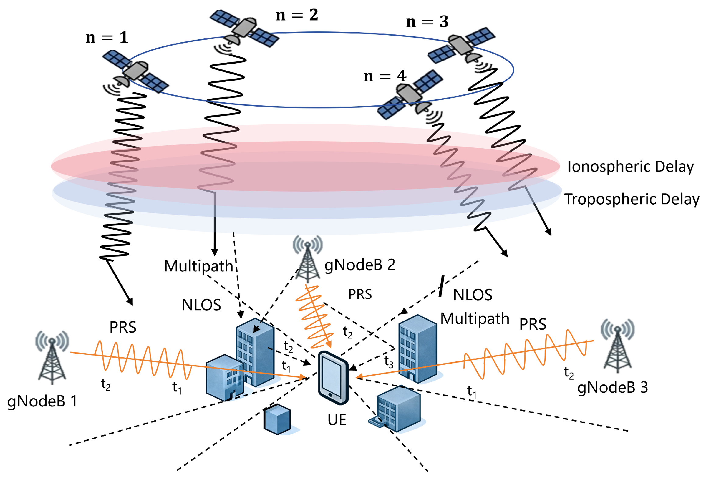
GNSS positioning estimates the receiver position from satellite observations. In open-sky environments, sufficient satellite visibility and favorable geometry usually lead to stable meter-level positioning. However, in dense urban environments, satellite blockage, multipath propagation, and reduced satellite visibility can significantly degrade the reliability of GNSS-derived position observations.

For the proposed fusion algorithm, GNSS errors are mainly considered from the perspective of observation reliability. Satellite-end errors, propagation-path errors, and receiver-end errors jointly affect the GNSS-derived position observation. Among these errors, multipath propagation and signal blockage are particularly important because they can produce abrupt position jumps and abnormal residuals. These abnormal GNSS observations are later detected using the Mahalanobis-distance criterion combined with INS-based motion-continuity constraints.

In addition, the number of visible GNSS satellites is used as a direct indicator of GNSS observation availability. A larger number of visible satellites generally improves geometric redundancy and positioning reliability, whereas a small number of satellites indicates degraded or unreliable GNSS observations. Therefore, the satellite number $N_{g,k}$ is used in the observation-quality-aware covariance-regulation strategy in Section 2.4.

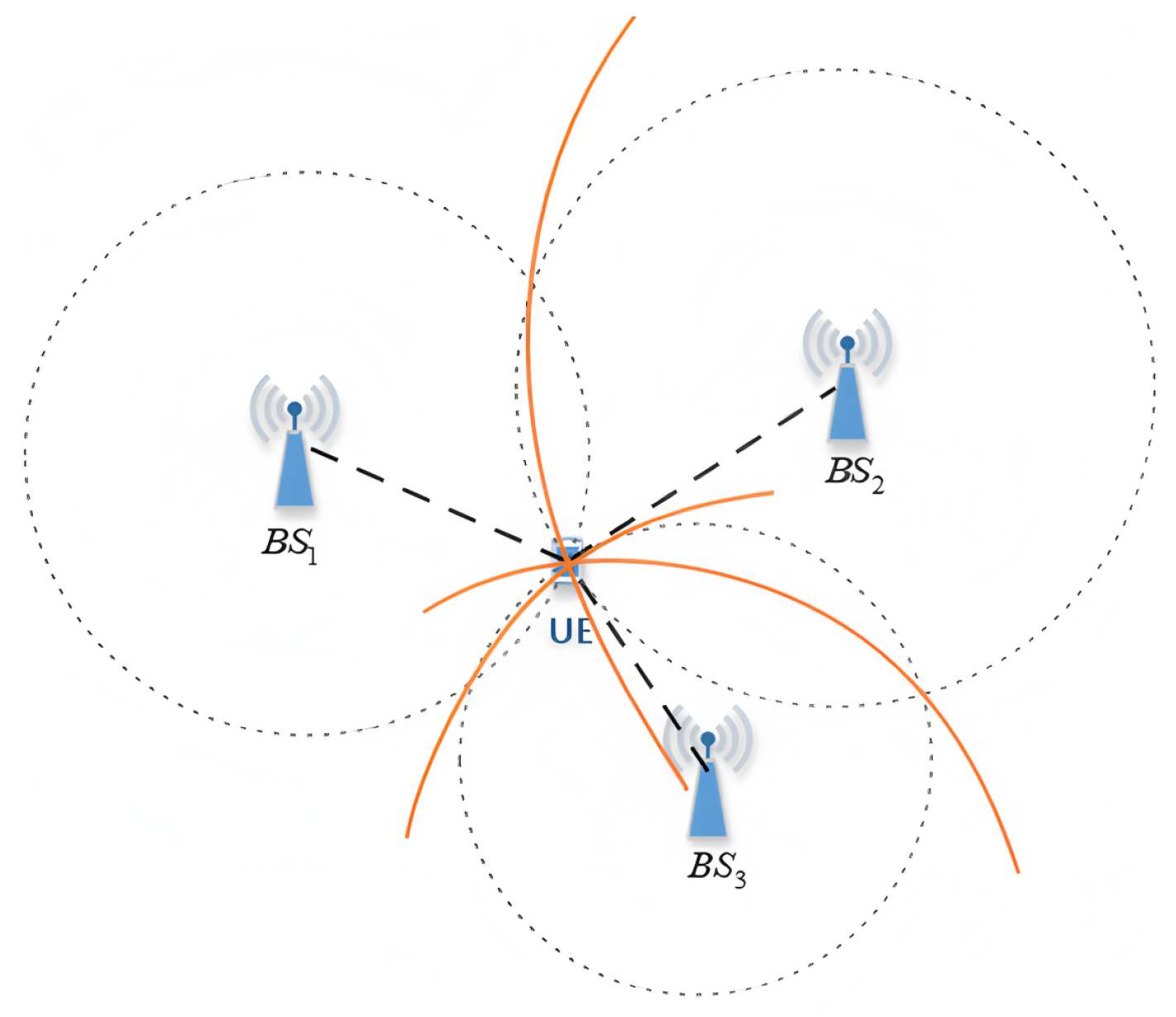
In this study, the 5G positioning subsystem provides TDOA-based position observations derived from PRS measurements. The gNodeBs transmit PRS signals, the UE measures arrival-time differences, and the LMF estimates the terminal position. The resulting 5G-derived position observation is then used as one measurement source in the proposed GNSS/5G/INS fusion framework. Figure 2 shows the schematic diagram of the TDOA positioning principle.

The reliability of 5G-derived position observations is affected by base-station availability, synchronization accuracy, NLOS propagation, multipath effects, terminal measurement noise, and base-station coordinate error. Among these factors, NLOS and multipath errors are dominant in dense urban and indoor environments because they can introduce biased or abruptly varying range-difference measurements. The total 5G observation error can be summarized as

$$\Delta {\rho }_{5\mathrm{G},k}=\Delta d_{\mathrm{sync},k}+\Delta d_{\mathrm{mp},k}+\Delta d_{\mathrm{NLOS},k}+\Delta d_{\mathrm{ue},k}+\Delta d_{\mathrm{bs},k}.$$

(1)

where $\Delta d_{\mathrm{sync},k}$ denotes the base-station synchronization error, $\Delta d_{\mathrm{mp},k}$ denotes the multipath-induced error, $\Delta d_{\mathrm{NLOS},k}$ denotes the NLOS error, $\Delta d_{\mathrm{ue},k}$ denotes the terminal measurement error, and $\Delta d_{\mathrm{bs},k}$ denotes the base-station coordinate error.

These error characteristics motivate two subsequent designs in the proposed method. First, abnormal GNSS and 5G observations are detected using statistical residual information and INS-based motion-continuity constraints. Second, the observation availability indicators $N_{g,k}$ and $N_{5,k}$ are used to dynamically regulate the relative confidence assigned to the external measurement sources, namely GNSS and 5G, in the UKF measurement update. INS is not assigned an observation-quality weight in this module; instead, it contributes through state prediction and INS-based motion-continuity constraints.

2.2. Overall Framework of the Proposed Fusion Method

This study develops a hierarchical fusion positioning framework composed of three modules: multi-sensor data preprocessing and error suppression, robust UKF-based nonlinear state estimation, and observation-quality-aware adaptive weighting. Using GNSS, 5G, and INS observations as inputs, the framework produces accurate and robust position estimates through the interaction of the three modules. First, the preprocessing layer reduces systematic sensor bias and random gross errors, thereby providing reliable observations for subsequent fusion. Second, the UKF filtering layer introduces a scenario-based state transition model and an adaptive sigma-point shrinkage mechanism, which can accurately handle the nonlinear characteristics of inertial navigation integration and sensor observation mapping, while suppressing filtering divergence caused by abnormal observations. Finally, the observation-quality-aware adaptive weighting layer dynamically regulates the effective measurement weights of GNSS and 5G based on the number of visible GNSS satellites and available 5G base stations, enabling smooth measurement-confidence transitions among open, semi-occluded, and fully occluded scenarios.

The novelty of the proposed framework lies in the closed-loop interaction among the three modules. The preprocessing module does not simply remove outliers independently; instead, it provides reliability-enhanced observations for the robust UKF. The UKF module further evaluates the innovation consistency and adaptively shrinks the sigma-point covariance when abnormal residuals occur. The weighting module then adjusts the external-observation confidence according to GNSS and 5G availability, ensuring that the final posterior estimate is obtained through quality-aware UKF measurement updating rather than a simple post-filter weighted average.

To avoid ambiguity, the proposed hierarchical fusion framework does not perform a secondary post-filter weighted average of standalone GNSS, 5G, and INS positioning results. Instead, GNSS- and 5G-derived position observations are used as measurement inputs of the UKF, while INS information is used for state prediction. The observation-quality-aware weights are introduced into the UKF by adaptively adjusting the effective measurement covariance matrices. Therefore, the final positioning output is the posterior position estimate extracted from the UKF state vector.

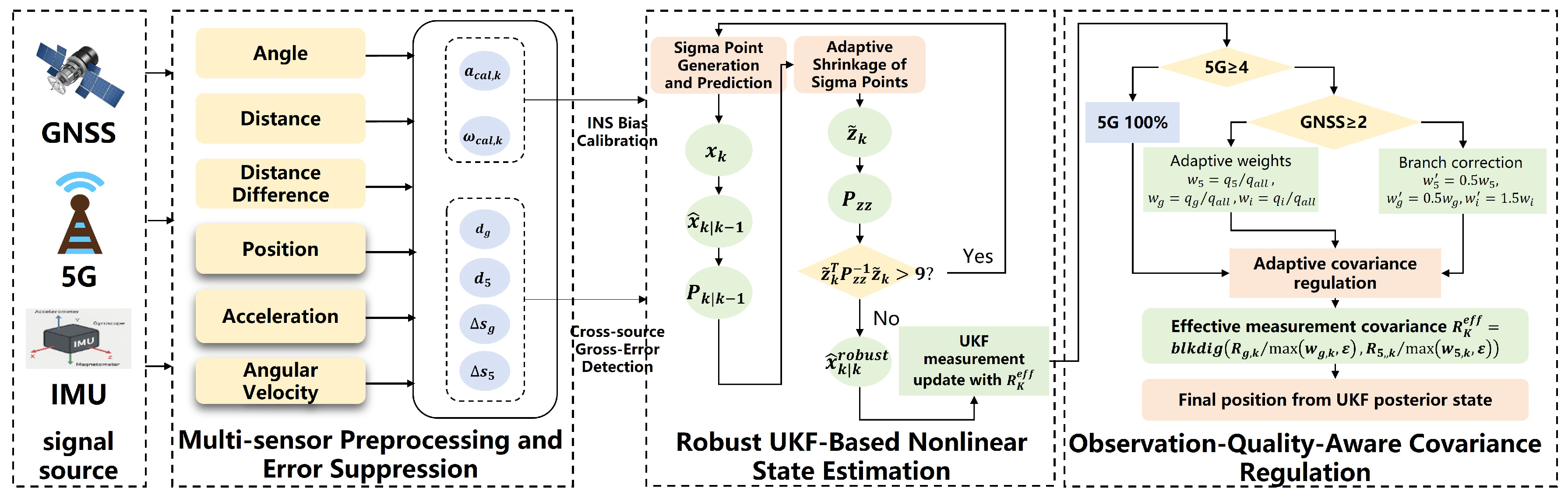
The following subsections describe the theoretical models, key equations, and implementation details of each module. Figure 3 shows the overall framework diagram of the algorithm.

The left module performs multi-sensor data preprocessing and error suppression using GNSS, 5G, and INS observations as inputs. Through real-time bias calibration and cross-source gross-error detection, this module provides reliable observations for subsequent fusion. The middle module performs robust UKF-based nonlinear state estimation using the preprocessed multi-sensor data. First, it performs sigma point generation and prediction to obtain predicted states and predicted observations. Then, an adaptive sigma-point shrinkage mechanism is introduced: by comparing the observation residuals with statistically determined chi-square thresholds, it adaptively selects either actual observations or predicted values to participate in the update process. Finally, it completes UKF state estimation, achieving accurate processing of nonlinear characteristics such as INS integration and sensor observation mapping, while suppressing filtering divergence caused by abnormal observations. The right module implements observation-quality-aware covariance regulation. Based on the numbers of available GNSS satellites and 5G base stations, this module dynamically adjusts the effective measurement confidence of GNSS and 5G. INS is not treated as an independent weighted positioning source; rather, it supports the UKF through state prediction and motion-continuity constraints.

For clarity, the GNSS-derived and 5G-derived position observations at epoch k are denoted as ${\mathbf{p}}_{g,k}$ and ${\mathbf{p}}_{5,k}$, respectively. The INS mechanization-derived position prediction is denoted as ${\mathbf{p}}_{I,k}$. It should be noted that ${\mathbf{p}}_{I,k}$ is not used as an independent post-filter positioning solution for final weighted averaging. In the proposed implementation, INS mechanization provides the state prediction and motion constraint for the UKF. The notation ${\mathbf{p}}_{I,k}$ is used only to represent the INS-predicted position component before measurement correction. The UKF state vector and its posterior estimate are denoted as ${\mathbf{x}}_k$ and ${\widehat{\mathbf{x}}}_{k|k}$, respectively. The position component extracted from the posterior state estimate is denoted as ${\widehat{\mathbf{p}}}_{k|k}$.

2.3. Dual-Domain Error Suppression

Inertial navigation was originally developed for military applications such as missiles, aircraft, and ships, utilizing inertial sensors including accelerometers and gyroscopes. Inertial sensors can be classified into navigation-grade, tactical-grade, industrial-grade, and consumer-grade sensors, with significant differences in their performance and cost. Inertial navigation uses measurements from accelerometers and gyroscopes to estimate the position, velocity, and attitude of a platform through algorithms such as INS mechanization, PDR, and motion constraints. In inertial navigation algorithms, because of inertial-sensor errors and integration errors, INS accuracy gradually degrades over time. By using self-contained inertial sensors, inertial navigation is independent of any external information and thus immune to external electromagnetic interference. It can be applied in various environments including aerial, terrestrial, and underwater scenarios, and is suitable for both vehicles and pedestrians. Inertial navigation provides position, velocity, and attitude solutions with high update rates, short-term accuracy, and good stability, but its drawback is that navigation errors accumulate over time, resulting in poor long-term accuracy.

The core principle of inertial navigation is to measure the motion states of the carrier (i.e., velocity and angular velocity) via inertial sensors (i.e., accelerometers and gyroscopes), and calculate the real-time position, velocity, and attitude of the carrier through integral operations based on Newton’s laws of motion. Essentially, it autonomously infers the motion trajectory relying solely on internal sensors without depending on external signals. The inertial navigation calculation consists of three steps: (1) attitude update, (2) velocity update, and (3) position update.

Attitude update calculates the attitude of the carrier in the navigation frame by measuring the angular velocity (unit: rad/s) of the carrier relative to the inertial frame using gyroscopes. The differential equation of the attitude angle can be obtained as follows:

$$\left\{\begin{array}{c}\dot{\varphi }=w_x+\sin \varphi \tan \theta ·w_y+\cos \varphi \tan \theta ·w_z\hfill \\ \dot{\theta }=\cos \varphi ·w_y-\sin \varphi ·w_z\hfill \\ \dot{\psi }={\displaystyle \frac{\sin \varphi }{\cos \theta }}{\omega }_y+{\displaystyle \frac{\cos \varphi }{\cos \theta }}{\omega }_z\hfill \end{array}\right.$$

(2)

where $w_x$, $w_y$, and $w_z$ are the angular velocities measured by the gyroscope in the body frame; $\dot{\varphi }$, $\dot{\theta }$, and $\dot{\psi }$ are the rates of change of the attitude angles. By integrating the above equations, the real-time attitude angles $\varphi \left(t\right)$, $\theta \left(t\right)$, and $\psi \left(t\right)$ can be obtained.

Velocity calculation involves measuring the specific force of the carrier via the accelerometer, transforming it to the navigation frame, subtracting the gravitational acceleration to derive the true acceleration, and then performing integration to calculate the velocity. The transformation of the specific force from the body frame to the navigation frame is expressed as follows:

$${\mathbf{f}}^n={\mathbf{C}}_{bn}·{\mathbf{f}}^b$$

(3)

where ${\mathbf{f}}^{\mathbf{b}}={[fx,fy,fz]}^T$ is the measured value of the accelerometer in the body frame, ${\mathbf{C}}_{\mathbf{bn}}$ is the attitude matrix, and ${\mathbf{f}}^{\mathbf{n}}$ is the specific force in the navigation frame.

Then the acceleration in the navigation frame is calculated as follows:

$${\dot{\mathbf{v}}}^{\mathbf{n}}={\mathbf{f}}^{\mathbf{n}}-{\mathbf{g}}^{\mathbf{n}}$$

(4)

where ${\mathbf{g}}^{\mathbf{n}}={\left[0,0,g\right]}^T$ denotes the gravitational acceleration in the navigation frame, and ${\dot{\mathbf{v}}}^n={\left[{\dot{v}}_E,{\dot{v}}_N,{\dot{v}}_U\right]}^{\mathrm{T}}$ represents the acceleration in the navigation frame.

Finally, the velocity is obtained by integrating the acceleration, which is expressed as follows:

$${\mathbf{v}}^n\left(t\right)={\mathbf{v}}^n\left(0\right)+{\int }_0^t{\dot{\mathbf{v}}}^n\left(\tau \right)\mathrm{d}\tau$$

(5)

where $v^n\left(0\right)$ is the initial velocity, and ${\mathbf{v}}^n\left(t\right)$ is the velocity at time $\mathbf{t}$.

Position is calculated by integrating velocity with respect to time. In the local navigation frame, the position is represented by latitude L, longitude $\lambda$, and height h, which can be obtained from the following position differential equations:

$$\left\{\begin{array}{c}\dot{L}={\displaystyle \frac{v_N}{R+h}}\hfill \\ \dot{\lambda }={\displaystyle \frac{v_E}{(R+h)\cos L}}\hfill \\ \dot{h}=v_U\hfill \end{array}\right.$$

(6)

where R is the Earth radius, and $\dot{L}$, $\dot{\lambda }$, and $\dot{h}$ are the rates of change of latitude, longitude, and height, respectively.

By integrating the above equations, the final position result can be obtained, which is expressed as follows:

$$L\left(t\right)=L\left(0\right)+{\int }_0^t\dot{L}\left(\tau \right)d\tau$$

(7)

$$\lambda \left(t\right)=\lambda \left(0\right)+{\int }_0^t\dot{\lambda }\left(\tau \right)d\tau$$

(8)

$$h\left(t\right)=h\left(0\right)+{\int }_0^t\dot{h}\left(\tau \right)d\tau$$

(9)

INS biases are systematic errors of inertial sensors. In static/low-dynamic scenarios, the true acceleration $a_{true}\approx 0$ and angular velocity ${\omega }_{true}\approx 0$ of the carrier are approximately zero, where the sensor output is approximately equal to the bias and can be estimated via statistical methods.

Static or low-dynamic states can be detected by calculating the variance of the INS acceleration data within a sliding window:

$${\sigma }_a^2={\displaystyle \frac{1}{N-1}}{\displaystyle \sum _{k=t-N+1}^t}{({\mathbf{a}}_k-\overline{\mathbf{a}})}^T({\mathbf{a}}_k-\overline{\mathbf{a}}),\overline{a}={\displaystyle \frac{1}{N}}{\displaystyle \sum _{k=t-N+1}^t}{a}_k$$

(10)

The state is determined to be static or low-dynamic when ${\sigma }_a^2<{\delta }_a$, where ${\delta }_a$ is the threshold.

The threshold ${\delta }_a$ was determined from the stationary calibration data collected before each experiment. Specifically, the variance of the accelerometer output was calculated over a stationary segment, and ${\delta }_a$ was set as

$${\delta }_a=c_a{\sigma }_{a,\mathrm{static}}^2,$$

where ${\sigma }_{a,\mathrm{static}}^2$ denotes the accelerometer variance during the stationary calibration period and $c_a$ is a safety coefficient. In this study, $c_a=2.5$ was used to avoid falsely classifying low-dynamic motion as a stationary state.

Bias estimation is implemented in static scenarios. The sensor output is expressed as ${\mathbf{a}}_k={\mathbf{b}}_a+{\mathbf{n}}_a$, where ${\mathbf{a}}_k\in {\mathbb{R}}^3$ is the accelerometer output vector, ${\mathbf{b}}_a\in {\mathbb{R}}^3$ is the accelerometer bias vector, and ${\mathbf{n}}_a$ is the accelerometer noise vector.

The accelerometer bias can be obtained by calculating the window average as follows:

$${\widehat{\mathbf{b}}}_a=\overline{\mathbf{a}}={\displaystyle \frac{1}{N}}{\displaystyle \sum _{k=t-N+1}^t}{\mathbf{a}}_k$$

(11)

Similarly, the gyroscope bias can be obtained via estimation as follows:

$${\widehat{\mathbf{b}}}_g=\overline{\mathsf{\omega }}={\displaystyle \frac{1}{N}}{\displaystyle \sum _{k=t-N+1}^t}{\mathsf{\omega }}_k$$

(12)

where ${\widehat{\mathbf{b}}}_g\in {\mathbb{R}}^3$ denotes the gyroscope bias.

Then, the calibrated INS data can be obtained as follows:

$${\mathbf{a}}_{\mathrm{cal},k}={\mathbf{a}}_k-{\widehat{\mathbf{b}}}_a$$

(13)

$${\mathsf{\omega }}_{\mathrm{cal},k}={\mathsf{\omega }}_k-{\widehat{\mathbf{b}}}_g$$

(14)

The calibration reduces systematic INS bias, which is a major source of long-term drift. The calibrated INS data are closer to the true motion state and provide more reliable inputs for subsequent UKF-based state estimation.

Gross errors refer to abnormal observations that deviate significantly from the normal observation distribution. The Mahalanobis distance quantifies the deviation between the current observation and the historical normal observation set. In addition, physical motion continuity is used as a consistency constraint: GNSS/5G observation jumps should be consistent with the INS-derived displacement.

Let the GNSS historical normal observation set be ${z_g^{\left(i\right)}}_{i=1}^M$, where M denotes the size of the historical window. The mean and covariance can be obtained, respectively, as follows:

$${\overline{\mathbf{z}}}_{g,k}={\displaystyle \frac{1}{M}}{\displaystyle \sum _{i=1}^M}{\mathbf{z}}_g^{\left(i\right)},{\mathbf{C}}_{g,k}={\displaystyle \frac{1}{M-1}}{\displaystyle \sum _{i=1}^M}\left({\mathbf{z}}_g^{\left(i\right)}-{\overline{\mathbf{z}}}_{g,k}\right){\left({\mathbf{z}}_g^{\left(i\right)}-{\overline{\mathbf{z}}}_{g,k}\right)}^T$$

(15)

By statistically analyzing the past M normal GNSS observation data, a baseline model for the normal observation state is established.

The squared Mahalanobis statistic of the current GNSS observation is expressed as

$${\mathcal{M}}_{g,k}={\tilde{\mathbf{z}}}_{g,k}^{\mathrm{T}}{\mathbf{C}}_{g,k}^{-1}{\tilde{\mathbf{z}}}_{g,k}.$$

(16)

Similarly, the squared Mahalanobis statistic for the 5G observation is

$${\mathcal{M}}_{5,k}={\tilde{\mathbf{z}}}_{5,k}^{\mathrm{T}}{\mathbf{C}}_{5,k}^{-1}{\tilde{\mathbf{z}}}_{5,k}.$$

(17)

where ${\tilde{\mathbf{z}}}_{g,k}={\mathbf{z}}_{g,k}-{\overline{\mathbf{z}}}_g$ and ${\tilde{\mathbf{z}}}_{5,k}={\mathbf{z}}_{5,k}-{\overline{\mathbf{z}}}_5$ are the residuals with respect to the historical normal baselines, and ${\mathbf{C}}_{g,k}$ and ${\mathbf{C}}_{5,k}$ denote the corresponding covariance matrices of the historical normal observation sets.

Unlike Euclidean distance, the Mahalanobis distance incorporates the covariance of the historical observation set and is therefore more appropriate for residual distributions with unequal variance and inter-dimensional correlation.

These squared Mahalanobis statistics quantify the deviation of the current GNSS and 5G observations from their historical normal baselines. They are then combined with the normal fluctuation range to identify abnormal observations.

A consistency judgment is performed on the INS motion, and the INS reckoning step size is expressed as follows:

$$\Delta {\mathbf{s}}_{I,k}={\int }_{t-\Delta t}^t{\mathbf{v}}_I\left(\tau \right)d\tau$$

(18)

where ${\mathbf{v}}_I\left(\tau \right)$ denotes the INS-derived velocity vector at time $\tau$.

The GNSS observation jump is defined as follows:

$$\Delta {\mathbf{s}}_{g,k}={\mathbf{p}}_{g,k}-{\mathbf{p}}_{g,k-1}$$

(19)

The position difference between two consecutive GNSS observations is used to represent the GNSS-derived displacement over the interval.

Similarly, the 5G observation jump is defined as

$$\Delta {\mathbf{s}}_{5,k}={\mathbf{p}}_{5,k}-{\mathbf{p}}_{5,k-1}$$

(20)

Here, ${\mathbf{z}}_{g,k}$ and ${\mathbf{z}}_{5,k}$ denote the GNSS and 5G measurement vectors; when the measurement vector is represented in position form, they correspond to ${\mathbf{p}}_{g,k}$ and ${\mathbf{p}}_{5,k}$, respectively.

Based on this displacement comparison, the consistency judgment can be obtained as follows:

$$\parallel \Delta {\mathbf{s}}_{j,k}\parallel \le \gamma \parallel \Delta {\mathbf{s}}_{I,k}\parallel ,j\in \{g,5\}.$$

(21)

where $\gamma$ is the threshold. The tolerance coefficient $\gamma$ accounts for the short-term uncertainty of INS mechanization and the possible time synchronization error between external observations and INS data. A value slightly larger than 1 allows normal dynamic motion and small INS integration errors, whereas an excessively large value may allow abnormal GNSS/5G jumps to pass the consistency test. In this study, $\gamma =1.5$ was selected based on a preliminary calibration segment. This value provides a practical tolerance for short-term INS integration errors and small time-synchronization deviations while still preventing large GNSS/5G jumps from entering the subsequent fusion process.

By comparing the moving distance derived from GNSS observations with the INS-reckoned distance, it is determined whether the GNSS observations are consistent with the INS-derived motion, thereby preventing abnormal observation jumps from entering the fusion process.

The Mahalanobis distance is adopted in this study because it accounts for the covariance structure of historical observations and provides a lightweight statistical criterion for abnormal-observation detection without requiring labeled training data. Compared with simple Euclidean-distance or fixed-threshold residual tests, it is more suitable for multi-source positioning observations whose uncertainty varies with satellite visibility, base-station availability, and environmental occlusion. Compared with learning-based outlier detectors, it has lower computational complexity and is more appropriate for real-time GNSS/5G/INS fusion scenarios with limited training data and rapidly changing observation conditions.

However, the Mahalanobis-distance criterion alone may still produce false alarms when the platform undergoes rapid motion or when short-term observation fluctuations are caused by dynamic environmental changes rather than true gross errors. Therefore, this study further introduces INS-based motion-continuity constraints to assist abnormal-observation identification. By jointly considering residual statistics and physically plausible motion continuity, the proposed method can better distinguish true GNSS/5G outliers from temporarily disturbed but still usable observations.

Therefore, in the proposed framework, the Mahalanobis-distance test serves as a computationally efficient first-stage gross-error screening tool, while INS continuity constraints and the subsequent adaptive fusion modules further improve robustness. Although other approaches, such as learning-based outlier detection or robust estimation methods, may also be applied, the Mahalanobis-distance test is selected here as a practical compromise between statistical rigor, computational efficiency, and real-time deployability.

Instead of using a fixed empirical Mahalanobis-distance threshold, the rejection threshold for the first-stage gross-error screening is determined from the chi-square distribution. For $j\in \{g,5\}$, the squared Mahalanobis statistic ${\mathcal{M}}_{j,k}$ is compared with

$$T_j^{\mathcal{M}}={\chi }_{m_j}^2(1-\alpha ),$$

(22)

where $m_j$ is the dimension of the corresponding observation vector and $\alpha$ is the significance level. In this study, $\alpha =0.01$ was used for gross-error rejection, corresponding to a 99% confidence level under the Gaussian residual assumption.

Therefore, the gross-error rejection rule is defined as

$${\mathcal{M}}_{j,k}>T_j^{\mathcal{M}}\mathrm{and}\parallel \Delta {\mathbf{s}}_{j,k}\parallel >\gamma \parallel \Delta {\mathbf{s}}_{I,k}\parallel ,j\in \{g,5\}.$$

(23)

If both conditions are satisfied, the corresponding GNSS or 5G observation ${\mathbf{z}}_{j,k}$ is rejected as a gross error before entering the UKF measurement update.

This method addresses the issue of random gross errors such as GNSS multipath interference and 5G NLOS errors, and prevents abnormal measurement vector from contaminating the UKF filtering process. In traditional filtering methods, gross errors in the input cause the state estimation to deviate drastically from the true value. Therefore, the proposed method ensures the reliability of the data source for subsequent fusion.

2.4. Adaptive-Shrinkage UKF and Quality-Aware Covariance Regulation

The UKF estimates nonlinear system states by propagating deterministically selected sigma points through the nonlinear state-transition and measurement functions. In this study, the standard UKF prediction-update structure is adopted, while robustness is enhanced through residual-driven sigma-point covariance shrinkage and quality-aware measurement covariance regulation.

The core states to be estimated by the fusion system are defined explicitly. The position, velocity, attitude angles required for positioning, as well as the key error sources of the inertial navigation system (INS) are integrated into a unified state vector. The fusion state is given by:

$${\mathbf{x}}_k={\left[{\mathbf{p}}_k^T,{\mathbf{v}}_k^T,{\varphi }_k^T,{\mathbf{b}}_{a,k}^T,{\mathbf{b}}_{g,k}^T\right]}^T$$

(24)

where ${\mathbf{p}}_k\in {\mathbb{R}}^3$ denotes the position, ${\mathbf{v}}_k\in {\mathbb{R}}^3$ denotes the velocity, ${\varphi }_k\in {\mathbb{R}}^3$ denotes the attitude-angle vector, and ${\mathbf{b}}_{a,k}\in {\mathbb{R}}^3$ and ${\mathbf{b}}_{g,k}\in {\mathbb{R}}^3$ denote the accelerometer bias and gyroscope bias, respectively.

The dynamic evolution law of the system state is described by the state transition model:

$${\mathbf{x}}_k=\mathbf{A}{\mathbf{x}}_{k-1}+\mathbf{B}{\mathbf{u}}_k+{\mathbf{w}}_{k-1}$$

(25)

where $\mathbf{A}$ is the state-transition matrix, $\mathbf{B}$ is the control-input matrix, ${\mathbf{u}}_k$ is the control-input vector, and ${\mathbf{w}}_{k-1}$ is the process-noise vector. This model quantifies the state transition from time $k-1$ to k, and the introduction of process noise reflects the uncertainty of the system dynamic model.

To address the nonlinear characteristics of the positioning system, the UKF generates $2n+1$ sigma points to approximate the Gaussian distribution of the state. Here, n denotes the dimension of the state vector. Since the proposed fusion state contains position, velocity, attitude angles, accelerometer bias, and gyroscope bias, $n=15$, and thus $2n+1=31$ sigma points are generated at each epoch. The term $2n+1$ is dimensionless because it denotes the number of deterministic sampling points rather than a physical measurement.

Based on ${\widehat{\mathbf{x}}}_{k-1|k-1}$ and ${\mathbf{P}}_{k-1|k-1}$, $2n+1$ sigma points can be generated as follows:

$$\left\{\begin{array}{c}{\mathbf{x}}_{k-1|k-1}^{\left(0\right)}={\widehat{\mathbf{x}}}_{k-1|k-1}\hfill \\ {\mathbf{x}}_{k-1|k-1}^{\left(i\right)}={\widehat{\mathbf{x}}}_{k-1|k-1}+{\left(\sqrt{(n+\lambda ){\mathbf{P}}_{k-1|k-1}}\right)}^{\left(i\right)},(i=1,2,\dots ,n)\hfill \\ {\mathbf{x}}_{k-1|k-1}^{(i+n)}={\widehat{\mathbf{x}}}_{k-1|k-1}-{\left(\sqrt{(n+\lambda ){\mathbf{P}}_{k-1|k-1}}\right)}^{\left(i\right)},(i=1,2,\dots ,n)\hfill \end{array}\right.$$

(26)

The generated sigma points are substituted into the nonlinear state equation to complete state prediction. The predicted state mean and covariance are then obtained as follows:

$${\mathbf{x}}_{k|k-1}^{\left(i\right)}=f\left({\mathbf{x}}_{k-1|k-1}^{\left(i\right)},{\mathbf{u}}_k\right),i=0,1,\dots ,2n$$

(27)

The a priori state mean is calculated as:

$${\widehat{\mathbf{x}}}_{k|k-1}={\displaystyle \sum _{i=0}^{2n}}{W}_m^{\left(i\right)}{\mathbf{x}}_{k|k-1}^{\left(i\right)}$$

(28)

The a priori covariance matrix is calculated as:

$${\mathbf{P}}_{k|k-1}={\displaystyle \sum _{i=0}^{2n}}{W}_c^{\left(i\right)}\left({\mathbf{x}}_{k|k-1}^{\left(i\right)}-{\widehat{\mathbf{x}}}_{k|k-1}\right){\left({\mathbf{x}}_{k|k-1}^{\left(i\right)}-{\widehat{\mathbf{x}}}_{k|k-1}\right)}^T+\mathbf{Q}$$

(29)

When the normalized innovation squared statistic exceeds the chi-square threshold, an observation anomaly or model mismatch is indicated.

We substitute the a priori predicted sigma points into the observation function and then obtain the theoretically expected measurement vector through weighting, i.e., the observation baseline predicted based on system dynamics. The predicted measurement vector is:

$${\widehat{\mathbf{z}}}_{k|k-1}={\displaystyle \sum _{i=0}^{2n}}{W}_m^{\left(i\right)}h\left({\mathbf{x}}_{k|k-1}^{\left(i\right)}\right).$$

(30)

where h denotes the observation function.

We subtract the predicted measurement vector from the current actual measurement vector to calculate the gap between the actual observation and the theoretical prediction. A smaller gap indicates a better match between the observation and the system dynamics; a larger gap may indicate observation anomalies.

The UKF measurement vector is constructed from the available external position observations after preprocessing and gross-error screening. When both GNSS and 5G observations are available, the measurement vector is defined as

$${\mathbf{z}}_k=\left[\begin{array}{c}{\mathbf{p}}_{g,k}\\ {\mathbf{p}}_{5,k}\end{array}\right].$$

(31)

$$\mathbf{h}\left({\mathbf{x}}_k\right)=\left[\begin{array}{c}{\mathbf{E}}_p{\mathbf{x}}_k\\ {\mathbf{E}}_p{\mathbf{x}}_k\end{array}\right],{\mathbf{E}}_p=\left[\begin{array}{cc}{\mathbf{I}}_3& {\mathbf{0}}_{3\times 12}\end{array}\right],$$

(32)

where ${\mathbf{E}}_p$ is the position extraction matrix. If either GNSS or 5G observations are unavailable or rejected by the gross-error test, the corresponding rows are removed from ${\mathbf{z}}_k$ and $\mathbf{h}\left({\mathbf{x}}_k\right)$.

Therefore, GNSS and 5G observations are incorporated as external measurement updates, whereas INS contributes to the UKF through state prediction and motion constraints rather than as an independent post-filter position solution.

The residual formula is:

$${\tilde{\mathbf{z}}}_k={\mathbf{z}}_k-{\widehat{\mathbf{z}}}_{k|k-1}$$

(33)

We calculate the uncertainty of this gap, i.e., the fluctuation range that the gap should have under normal conditions. The residual covariance is:

$${\mathbf{P}}_{zz,k}={\displaystyle \sum _{i=0}^{2n}}{W}_c^{\left(i\right)}\left({\mathbf{z}}_{k|k-1}^{\left(i\right)}-{\widehat{\mathbf{z}}}_{k|k-1}\right){\left({\mathbf{z}}_{k|k-1}^{\left(i\right)}-{\widehat{\mathbf{z}}}_{k|k-1}\right)}^T+\mathbf{R}$$

(34)

To avoid the arbitrariness of a fixed $3\sigma$ threshold, the UKF innovation consistency test is performed using the normalized innovation squared (NIS) statistic. For $j\in \{g,5\}$, the innovation vector is defined as

$${\mathbf{r}}_{j,k}={\mathbf{z}}_{j,k}-{\widehat{\mathbf{z}}}_{j,k|k-1}.$$

(35)

The NIS statistic is calculated as

$${\mathcal{N}}_{j,k}={\mathbf{r}}_{j,k}^{\mathrm{T}}{\mathbf{S}}_{j,k}^{-1}{\mathbf{r}}_{j,k},$$

(36)

where ${\mathbf{S}}_{j,k}$ denotes the innovation covariance matrix corresponding to the j-th observation source, which is obtained from the corresponding block of ${\mathbf{P}}_{zz,k}$. Under the Gaussian innovation assumption, ${\mathcal{N}}_{j,k}$ approximately follows a chi-square distribution with $m_j$ degrees of freedom. Therefore, the detection threshold is defined as

$$T_j^{\mathcal{N}}={\chi }_{m_j}^2(1-\alpha ).$$

(37)

If ${\mathcal{N}}_{j,k}>T_j^{\mathcal{N}}$, the corresponding observation is regarded as degraded and its measurement covariance is inflated before the UKF measurement update.

When an observation anomaly occurs, a shrinkage factor ${\eta }_s\in (0,1]$ is introduced to adjust the sigma-point covariance:

$${\mathbf{P}}_{k|k-1}^{\mathrm{shrink}}={\eta }_s{\mathbf{P}}_{k|k-1}.$$

Here, ${\eta }_s$ controls the conservativeness of the UKF prediction under abnormal innovations. A smaller ${\eta }_s$ reduces the influence of abnormal observations more strongly but may also weaken the filter’s responsiveness to real motion changes. In this study, ${\eta }_s=0.5$ is used as a conservative shrinkage factor. This setting reduces the influence of abnormal observations while retaining sufficient filter responsiveness to normal motion changes.

We regenerate sigma points based on the shrunk covariance and repeat the prediction and update steps to obtain the robust state estimate, i.e.,

$${\widehat{\mathbf{x}}}_{k|k}^{\mathrm{robust}}={\widehat{\mathbf{x}}}_{k|k-1}+{\mathbf{K}}_k^{\mathrm{shrink}}{\tilde{\mathbf{z}}}_k$$

(38)

where ${\mathbf{K}}_k^{\mathrm{shrink}}$ is the Kalman gain recalculated using the shrunk covariance ${\mathbf{P}}_{k|k-1}^{\mathrm{shrink}}$. This residual-driven shrinkage mechanism differs from the conventional UKF, where the sigma-point covariance is propagated using fixed noise assumptions. By adaptively reducing the predicted covariance under abnormal residuals, the proposed method limits the influence of unreliable observations on the posterior state update and improves filtering stability in NLOS or partially occluded environments.

To quantify the instantaneous reliability of the external measurement sources, the GNSS and 5G observation-quality scores are defined as

$$q_{g,k}=\min \left({\displaystyle \frac{N_{g,k}}{6}},1\right),q_{5,k}=\min \left({\displaystyle \frac{N_{5,k}}{4}},1\right),$$

where $N_{g,k}$ and $N_{5,k}$ denote the numbers of available GNSS satellites and available 5G base stations at epoch k, respectively. The threshold of six GNSS satellites is selected because at least four satellites are required for 3D positioning, while additional satellites improve geometric redundancy and observation reliability. The threshold of four 5G base stations corresponds to the minimum requirement for stable 3D TDOA positioning. Therefore, these thresholds are used to normalize the availability of GNSS and 5G observations into comparable quality scores.

It should be emphasized that the adaptive weights are not used to directly average standalone positioning results. Instead, the weights are introduced to regulate the effective measurement covariance matrices of GNSS and 5G in the UKF measurement update. In this way, external observations with higher reliability are assigned smaller equivalent covariance, while degraded observations are automatically down-weighted through covariance inflation.

After obtaining the preliminary observation quality scores, the normalized weights of GNSS and 5G are calculated as

$${\tilde{w}}_{g,k}={\displaystyle \frac{q_{g,k}}{q_{g,k}+q_{5,k}+\epsilon }},$$

(39)

$${\tilde{w}}_{5,k}={\displaystyle \frac{q_{5,k}}{q_{g,k}+q_{5,k}+\epsilon }},$$

(40)

where $q_{g,k}$ and $q_{5,k}$ denote the observation-quality scores of GNSS and 5G, respectively, and $ϵ={10}^{-6}$ is a small positive constant used only to avoid division by zero. Since $ϵ$ is several orders of magnitude smaller than the normalized quality scores, it has negligible influence when at least one external observation source is available.

To avoid abrupt changes in the measurement noise covariance, the normalized weights are smoothed as

$$w_{j,k}=\beta w_{j,k-1}+(1-\beta ){\tilde{w}}_{j,k},j\in \{g,5\}.$$

(41)

where $\beta =0.8$ is the smoothing coefficient. A larger $\beta$ produces smoother but slower weight transitions, whereas a smaller $\beta$ improves responsiveness but may introduce abrupt covariance changes. The value of $\beta =0.8$ is selected according to the sampling interval and the need to balance smooth covariance transitions with real-time responsiveness.

The smoothed weights are then used to construct the effective measurement covariance matrix:

$${\mathbf{R}}_k^{eff}=\mathrm{blkdiag}\left({\displaystyle \frac{{\mathbf{R}}_{g,k}}{\max (w_{g,k},\epsilon )}},{\displaystyle \frac{{\mathbf{R}}_{5,k}}{\max (w_{5,k},\epsilon )}}\right).$$

(42)

Therefore, the adaptive weighting mechanism affects the UKF update through the measurement covariance matrix rather than through a post-filter weighted average. The posterior state estimate is updated as

$${\widehat{\mathbf{x}}}_{k|k}={\widehat{\mathbf{x}}}_{k|k-1}+{\mathbf{K}}_k\left[{\mathbf{z}}_k-\mathbf{h}\left({\widehat{\mathbf{x}}}_{k|k-1}\right)\right],$$

(43)

where ${\mathbf{K}}_k$ is the Kalman gain computed using ${\mathbf{R}}_k^{eff}$. Since INS is used in the prediction model rather than in the external measurement vector, no INS-related block is included in ${\mathbf{R}}_k^{eff}$.

Finally, the positioning output is extracted from the posterior UKF state estimate:

$${\mathbf{p}}_{out,k}={\mathbf{E}}_p{\widehat{\mathbf{x}}}_{k|k},$$

(44)

where ${\mathbf{E}}_p$ is the selection matrix used to extract the position component. Thus, the final positioning result is generated by the UKF posterior estimate, not by directly averaging GNSS, 5G, and INS positioning results.

In this strategy, sensors with higher observation quality are assigned higher confidence during the UKF measurement update, which improves both positioning accuracy and scenario adaptability. The parameter settings used in the proposed method are summarized in

Table 1. Parameter settings of the proposed method.

Parameter	Value	Role and Selection Basis
$\alpha$	$0.01$	Chi-square gross-error detection; 99% confidence level
$\gamma$	$1.5$	INS motion-continuity tolerance; preliminary calibration
${\delta }_a$	$2.5{\sigma }_{a,\mathrm{static}}^2$	Static/low-dynamic detection; stationary INS calibration
${\eta }_s$	$0.5$	Conservative sigma-point covariance shrinkage
$N_g^{\mathrm{th}}$	6	GNSS availability normalization; 3D positioning redundancy
$N_5^{\mathrm{th}}$	4	5G availability normalization; 3D TDOA requirement
$\beta$	$0.8$	Weight smoothing; balance of smoothness and responsiveness
$\epsilon$	${10}^{-6}$	Numerical stability to avoid division by zero

.

The smoothed GNSS and 5G measurement weights in Equation (41) prevent abrupt changes in the effective measurement covariance matrix. When GNSS or 5G observations become degraded, their corresponding covariance terms are inflated, and the UKF posterior estimate relies relatively more on the INS-driven state prediction. This does not introduce a separate INS weight; rather, it reflects the prediction-update structure of the UKF.

2.5. Experimental Site, Data Collection Platform, and Evaluation Metrics

To evaluate the proposed hierarchical fusion positioning framework under different signal-obstruction conditions, real-world experiments were conducted at the Dongying Petrochemical Plant. The experimental site contains open outdoor areas, partially obstructed outdoor areas, and fully occluded indoor areas, making it suitable for evaluating the positioning performance of GNSS/5G/INS fusion in complex urban-like environments. The layout of the experimental site and the distribution of 5G base stations and reference markers are shown in Figure 4.

2.5.1. Experimental Site and Test Scenarios

Three representative test scenarios were designed.

Scenario 1 was an open outdoor environment in an unobstructed area of the plant site. In this scenario, the number of visible GNSS satellites was stable at 8–12, and the number of visible 5G base stations was 4–6.

Scenario 2 was a semi-occluded outdoor environment in a partially obstructed area of the plant site. In this scenario, the number of visible GNSS satellites fluctuated between 3 and 7, and the number of visible 5G base stations was 2–4. This scenario was designed to evaluate the robustness of the proposed method under partial GNSS blockage and 5G NLOS interference.

Scenario 3 was a fully occluded indoor environment, where GNSS signals were unavailable and the number of visible 5G base stations was 3–6. This scenario was used to verify whether the proposed method could maintain positioning continuity when GNSS observations were completely unavailable.

2.5.2. Reference Position Acquisition

To ensure the reliability of the accuracy evaluation in environments where RTK-GNSS is degraded or unavailable, different reference-position acquisition methods were adopted for different scenarios. In the open outdoor scenario, RTK-GNSS was used as the reference source because stable satellite visibility allowed continuous RTK positioning. In the semi-occluded outdoor and fully occluded indoor scenarios, a total station was used to survey physical reference markers before data collection. These markers were distributed along the test route and their coordinates were transformed into the same local coordinate frame as the positioning results.

During data collection, the terminal was placed successively at the surveyed reference markers, and positioning data were recorded at each marker. The reference position $p_{ref,n}$ used in the RMSE and MAE calculations was therefore the total-station-surveyed coordinate of the corresponding marker. In this way, the positioning errors in the semi-occluded and fully occluded indoor scenarios were evaluated using independent total-station reference points rather than RTK-GNSS results.

2.5.3. Multi-Sensor Data Collection Platform

A multi-sensor data collection system integrating GNSS, 5G, and INS was built.

• The GNSS module supports BeiDou Navigation Satellite System (BDS) B1C/B2a and Global Positioning System (GPS) L1C/L5 frequency bands, with a sampling rate of 1 Hz, and supports raw observation data output.
• The 5G module uses the ADRV9009 radio-frequency chip, (Analog Devices, Inc., Wilmington, MA, USA), supports a bandwidth of 100 MHz, and has a receiving sensitivity of −105 dBm and a noise figure of no more than 2 dB.
• The INS module has a sampling rate of 100 Hz, configurable up to 200 Hz, with an accelerometer bias of 0.005 m/s² and a gyroscope bias of 0.1°/h. It outputs raw inertial data via a Serial Peripheral Interface (SPI), integrates a one-pulse-per-second (1PPS) synchronization interface, and achieves a time synchronization accuracy of ≤1 μs.
• In the semi-occluded outdoor and fully occluded indoor scenarios, reference markers were surveyed using a CHCNAV CTS-112R4Pro total station. The instrument has an angular accuracy of ${2.0}^{″}$, a maximum reflectorless measurement range of 800 m, and a minimum distance display resolution of 0.1 mm. These specifications were used to establish high-precision reference marker coordinates for positioning-error evaluation.

2.5.4. Evaluation Metrics

To quantitatively evaluate the positioning performance, three core indicators commonly used in the positioning field are adopted, covering accuracy, robustness, and continuity:

$$\mathrm{RMSE}=\sqrt{{\displaystyle \frac{1}{N}}\sum _{n=1}^N{∥{\mathbf{p}}_{\mathrm{out},n}-{\mathbf{p}}_{\mathrm{ref},n}∥}^2}$$

(45)

$$\mathrm{MAE}={\displaystyle \frac{1}{N}}{\displaystyle \sum _{n=1}^N}∥{\mathbf{p}}_{\mathrm{out},n}-{\mathbf{p}}_{\mathrm{ref},n}∥$$

(46)

where N is the number of positioning samples, ${\mathbf{p}}_{out,n}$ is the estimated position at sample n, and ${\mathbf{p}}_{ref,n}$ is the corresponding reference position. Specifically, ${\mathbf{p}}_{ref,n}$ was obtained from RTK-GNSS in the open outdoor scenario and from total-station-surveyed physical markers in the semi-occluded outdoor and fully occluded indoor scenarios.

Robustness indicators: Include the standard deviation of positioning errors and the outlier tolerance rate, i.e., the RMSE growth ratio under abnormal observations, which reflect the algorithm’s resistance to interference.

Continuity indicators: Include the average number of positioning interruption events per trial and the interrupted-epoch rate. To avoid ambiguity, a positioning interruption event is defined as a continuous time interval during which the positioning system cannot provide a valid position solution, or the horizontal positioning error exceeds the predefined availability threshold $e_{\mathrm{th}}$. Consecutive interrupted epochs are counted as one interruption event rather than multiple independent events.

For the rth trial, the interruption indicator at epoch k is defined as

$$I_{r,k}=\left\{\begin{array}{cc}1,\hfill & \mathrm{if}\mathrm{the}\mathrm{position}\mathrm{solution}\mathrm{is}\mathrm{unavailable}\mathrm{or}\parallel {\mathbf{p}}_{out,r,k}-{\mathbf{p}}_{ref,r,k}\parallel >e_{\mathrm{th}},\hfill \\ 0,\hfill & \mathrm{otherwise}.\hfill \end{array}\right.$$

The number of interruption events in the rth trial is calculated as

$$C_r={\displaystyle \sum _{k=1}^{N_r}}\mathbb{I}\left(I_{r,k}=1\mathrm{and}(k=1\mathrm{or}{I}_{r,k-1}=0)\right),$$

where $N_r$ is the number of epochs in the rth trial. Thus, each $C_r$ is an integer, while the reported value in the tables is the average over ten trials:

$$\overline{C}={\displaystyle \frac{1}{R}}{\displaystyle \sum _{r=1}^R}{C}_r,R=10.$$

The standard deviation of interruption events across the ten trials is calculated as

$${\sigma }_C=\sqrt{{\displaystyle \frac{1}{R-1}}\sum _{r=1}^R{(C_r-\overline{C})}^2}.$$

The interrupted-epoch rate is defined as

$${\rho }_{\mathrm{int}}={\displaystyle \frac{{\sum }_{r=1}^R{\sum }_{k=1}^{N_r}{I}_{r,k}}{{\sum }_{r=1}^R{N}_r}}\times 100\%.$$

Therefore, the reported interruption count can be fractional because it represents the mean value over ten independent trials, whereas the interruption count in each individual trial remains an integer. In this study, $e_{\mathrm{th}}=5\mathrm{m}$ was used according to the positioning availability requirement.

Different experiment durations were used for different evaluation purposes. The 300 s semi-occluded outdoor experiment was used as the primary long-duration evaluation to capture intermittent GNSS blockage and dynamic 5G NLOS variations. The 100 s ablation experiment was used to compare the relative contribution of each module under the same semi-occluded outdoor condition, while the 30 s baseline comparison was used as a representative short-duration segment for comparing different filtering algorithms under identical data input. Therefore, results should be compared within the same table, where all algorithms share the same duration and data segment, rather than by directly comparing interruption counts across tables. To improve cross-duration comparability, the interrupted-epoch rate is reported together with the average number of interruption events. The fully occluded indoor trials lasted 30 s because the indoor test route was shorter and spatially constrained; the experiment was repeated ten times to ensure statistical reliability.

3. Results

3.1. Performance in the Open Outdoor Environment

Experiments were conducted in the open outdoor environment of the plant site. The experiment consisted of ten trials, and data were collected for 30 s in each trial. The results are presented in Figure 5 and

Table 2. Continuity comparison in the open outdoor environment.

Method	Interruption Events Per Trial (Mean ± SD)	Interrupted-Epoch Rate
GNSS-only	$1.1\pm 0.3$	0.33%
5G-only	$1.8\pm 0.5$	0.85%
Proposed method	$1.1\pm 0.3$	0.33%

.

Figure 5 compares the positioning performance of the GNSS-only, 5G-only, and proposed fusion methods in the open and unobstructed environment. The CDF curves show that the proposed method yields a more concentrated error distribution and smaller horizontal errors at the same cumulative probability. In the time-series plot of horizontal errors, its fluctuation amplitude is far lower than that of the GNSS-only and 5G-only schemes, indicating superior stability. The RMSE and MAE of the proposed method are 1.05 m and 0.50 m, respectively; compared with the GNSS-only scheme RMSE 1.14 m, MAE 1.01 m, the RMSE is reduced by approximately 7.9% and the MAE by approximately 50.5%. In contrast to the 5G-only scheme RMSE 1.40 m, MAE 1.22 m, the RMSE is reduced by approximately 25.0% and the MAE by approximately 59.0%. The proposed method has $1.1\pm 0.3$ interruption events per trial and an interrupted-epoch rate of 0.33%, which are consistent with those of the GNSS-only scheme. Compared with the 5G-only scheme, which has $1.8\pm 0.5$ interruption events per trial and an interrupted-epoch rate of 0.85%, the proposed method reduces the average number of interruption events by approximately 38.9% and the interrupted-epoch rate by approximately 61.2%.

3.2. Performance in the Semi-Occluded Outdoor Environment

Experiments were conducted in the semi-occluded outdoor environment of the plant site. The experiment consisted of ten trials, and data were collected for 300 s in each trial to capture intermittent signal blockage and dynamic observation changes. The results are presented in Figure 6 and

Table 3. Continuity comparison in the semi-occluded outdoor environment.

Method	Interruption Events Per Trial (Mean ± SD)	Interrupted-Epoch Rate
GNSS-only	$60.5\pm 5.2$	28.8%
5G-only	$36.6\pm 3.8$	12.6%
Proposed method	$19.6\pm 2.1$	8.1%

. This longer observation duration allows transient GNSS degradation events caused by partial blockage and multipath propagation to be observed more clearly in the time-series error curve.

Figure 6a shows two pronounced GNSS-only horizontal error peaks at approximately 50 s and 150 s. These two transient error events are mainly attributed to temporary satellite blockage and multipath propagation when the terminal passed through partially obstructed areas near plant facilities. In the semi-occluded outdoor scenario, the number of visible GNSS satellites fluctuated between three and seven, indicating unstable satellite geometry and intermittent GNSS availability. When satellite visibility temporarily decreased or multipath became stronger, the GNSS-only solution was more likely to produce abrupt horizontal error increases.

In contrast, the proposed method did not exhibit corresponding sharp error peaks at these two time instants. This is because the abnormal GNSS observations were suppressed by the cross-source gross-error detection and residual-driven UKF covariance regulation, while 5G observations and INS-driven state prediction helped maintain short-term positioning continuity. Therefore, the two GNSS-only error peaks in Figure 6a provide direct evidence that the proposed fusion method can mitigate transient GNSS degradation in semi-occluded outdoor environments.

According to Figure 6b, the proposed method achieves a horizontal RMSE of 1.54 m and a horizontal MAE of 1.36 m. Compared with the GNSS-only scheme, the RMSE and MAE are reduced by approximately 67.4% and 67.7%, respectively. Compared with the 5G-only scheme, the RMSE and MAE are reduced by approximately 45.2% and 41.1%, respectively. The proposed method has $19.6\pm 2.1$ interruption events per trial and an interrupted-epoch rate of 8.1%; compared with the GNSS-only scheme, the number of interruptions is reduced by approximately 67.6% and the interruption rate by approximately 71.9%. Relative to the 5G-only scheme, the number of interruptions is reduced by approximately 46.4% and the interruption rate by approximately 35.7%. The reduction in interruption events and interrupted-epoch rate also indicates that the proposed method is less affected by the transient GNSS degradation events observed around 50 s and 150 s in Figure 6a.

3.3. Performance in the Fully Occluded Indoor Environment

Experiments were conducted in the fully occluded indoor environment of the plant site. The experiment consisted of ten trials, and data were collected for 30 s in each trial. The results are presented in Figure 7 and

Table 4. Continuity comparison in the fully occluded indoor environment.

Method	Interruption Events Per Trial (Mean ± SD)	Interrupted-Epoch Rate
5G-only	$10.6\pm 1.1$	8.8%
Proposed method	$8.6\pm 0.9$	6.5%

.

In the fully occluded indoor environment of the plant site, GNSS signals are unavailable, leaving only 5G and INS for positioning. Figure 7 compares the positioning performance of the 5G-only scheme and the proposed method in the fully occluded indoor environment. The CDF curve of the proposed method shifts to the left, indicating smaller horizontal errors and a more concentrated error distribution. For the 5G-only scheme, the horizontal positioning RMSE and MAE are 2.49 m and 2.25 m, respectively; for the proposed fusion algorithm, the RMSE drops to 1.05 m and the MAE to 0.95 m. Compared with the 5G-only scheme, the RMSE and MAE are both reduced by approximately 57.8%. The 5G-only scheme has 10.6 interruptions and an 8.8% interruption rate, while the proposed fusion algorithm reduces the number of interruptions to 8.6 and the interruption rate to 6.5%. Relative to the 5G-only scheme, the number of interruptions is reduced by approximately 18.9%, and the interruption rate by approximately 26.1%.

3.4. Ablation Study

Experiments were conducted in the semi-occluded outdoor environment of the plant site. The ablation study used ten 100 s trials selected from the same semi-occluded outdoor test route. All ablation schemes were evaluated on the identical data segments, and therefore the results in Figure 8 and

Table 5. Continuity and error-stability comparison in the ablation experiments.

Different Algorithms	Interruption Events Per Trial (Mean ± SD)	Interrupted-Epoch Rate	Error STD (m)
Ablation 1	$10.6\pm 1.1$	5.6%	0.88
Ablation 2	$19.3\pm 1.9$	14.2%	1.25
Ablation 3	$25.8\pm 2.6$	22.8%	1.74
Complete proposed method	$6.5\pm 0.7$	2.1%	0.31

are comparable within this ablation experiment.

In this ablation experiment, the positioning performance of the complete proposed method and three ablation schemes was compared. The CDF curve of the complete proposed method is the leftmost: the cumulative probability approaches 1 when the error is less than 2 m; in contrast, Ablation 1 requires an error less than 4 m, Ablation 2 less than 6 m, and Ablation 3 less than 9 m to achieve the same cumulative probability, which demonstrates that the error distribution of the complete proposed method is more concentrated.

The horizontal RMSE and MAE of the complete proposed method are 1.68 m and 1.60 m, respectively. For Ablation 1, with an RMSE of 3.42 m and an MAE of 3.18 m, the complete proposed method reduces the RMSE by 50.9% and the MAE by 49.7%. For Ablation 2, with an RMSE of 5.97 m and an MAE of 5.76 m, the complete proposed method achieves reductions of 71.9% and 72.2% in RMSE and MAE, respectively. For Ablation 3, with an RMSE of 7.83 m and an MAE of 7.44 m, the complete proposed method reduces the RMSE and MAE by approximately 78.5% and 78.5%, respectively. The complete proposed method only has 6.5 interruptions with an interruption rate of 2.1%; compared with Ablation 1, which has an average of 10.6 interruptions per trial and a positioning interruption rate of 5.6%, the complete proposed method reduces the number of interruptions by 38.7% and the interruption rate by 62.5%. Compared with Ablation 3, which has an average of 25.8 interruptions per trial and a positioning interruption rate of 22.8%, the complete proposed method reduces the number of interruptions by 74.8% and the interruption rate by 90.8%. The RMSE curve of the complete proposed method remains consistently within the range of 1–2 m with minimal fluctuation; the fluctuation of the RMSE curves of the ablation schemes gradually increases as modules are removed. The standard deviation of the positioning error for the complete proposed method is 0.31 m, which is 64.8% lower than that of Ablation 1 and 82.2% lower than that of Ablation 3.

3.5. Comparison with Baseline Algorithms

Experiments were conducted in the semi-occluded outdoor environment of the plant site. The baseline-algorithm comparison used ten 30 s representative trials selected from the same semi-occluded outdoor test route. EKF/fixed-weight UKF, LSTM-aided UKF, and the proposed method were evaluated on the identical data segments. Therefore, the results in Figure 9 and

Table 6. Continuity and error-stability comparison of different algorithms in the semi-occluded outdoor environment.

Method	Interruption Events Per Trial (Mean ± SD)	Interrupted-Epoch Rate	Error STD (m)
EKF/fixed-weight UKF	$30.6\pm 3.2$	28.4%	1.43
LSTM-aided UKF	$24.8\pm 2.5$	18.6%	1.22
Proposed method	$18.6\pm 1.9$	9.4%	0.55

are intended for within-table algorithm comparison rather than direct comparison with the long-duration results in Figure 6 and Table 3.

By comparing the positioning performance of different algorithms with the proposed fusion algorithm in the semi-occluded outdoor environment of the plant site, it can be observed that the CDF curve of the proposed method shifts to the left, indicating a more concentrated error distribution and smaller positioning deviations. The cumulative probability approaches 1 when the error is less than 2 m, indicating a more concentrated error distribution and smaller positioning deviations in most scenarios. The error curve shows that the horizontal error fluctuation of the proposed method is significantly smaller than that of EKF/fixed-weight UKF and LSTM-aided UKF. In terms of error stability (STD), the proposed method has an error STD of 0.55 m, which is approximately 61.5% lower than that of EKF/fixed-weight UKF 1.43 m. The horizontal RMSE and MAE of EKF/fixed-weight UKF are 3.57 m and 3.01 m, respectively; those of LSTM-aided UKF are 2.38 m and 1.92 m, while the proposed method reduces the RMSE to 1.61 m and the MAE to 1.47 m. Compared with EKF/fixed-weight UKF, the RMSE is reduced by approximately 54.9% and the MAE by approximately 51.2%. The number of interruptions and interruption rate of EKF/fixed-weight UKF reach 30.6 times and 28.4%, respectively, whereas the proposed method decreases the number of interruptions to 18.6 times and the interruption rate to 9.4%. Relative to EKF/fixed-weight UKF, the number of interruptions is reduced by approximately 39.2% and the interruption rate by approximately 66.9%.

Compared with LSTM-aided UKF, the proposed method reduces the RMSE and MAE by approximately 32.4% and 23.4%, respectively. In addition, the average number of positioning interruptions and the positioning interruption rate are reduced by approximately 25.0% and 49.5%, respectively.

Experiments were conducted in the fully occluded indoor environment of the plant site. The experiment consisted of ten trials, and data were collected for 30 s in each trial. The results are presented in Figure 10 and

Table 7. Continuity and error-stability comparison in the fully occluded indoor environment.

Method	Interruption Events Per Trial (Mean ± SD)	Interrupted-Epoch Rate	Error STD (m)
EKF/fixed-weight UKF	$25.6\pm 2.6$	20.4%	1.36
LSTM-aided UKF	$19.8\pm 2.0$	12.6%	1.02
Proposed method	$10.6\pm 1.1$	5.4%	0.36

.

By comparing the positioning performance of different algorithms with the proposed fusion algorithm in the fully occluded indoor environment of the plant site, the CDF curve of the proposed method shifts to the left, indicating smaller horizontal errors. The cumulative probability approaches 1 when the horizontal error is less than 2 m, whereas the EKF/fixed-weight UKF requires an error greater than 2 m to achieve the same cumulative probability, indicating that the proposed method has a more concentrated error distribution and smaller positioning deviations in most scenarios. The error curve shows that the horizontal error fluctuation of the proposed method is significantly smaller than that of EKF/fixed-weight UKF and LSTM-aided UKF, remaining consistently within a low range.

In terms of error stability, the proposed method has a standard deviation of 0.36 m, which is approximately 73.5% lower than that of EKF/fixed-weight UKF and approximately 64.7% lower than that of LSTM-aided UKF. The horizontal RMSE and MAE of EKF/fixed-weight UKF are 3.08 m and 2.63 m, respectively; those of LSTM-aided UKF are 2.16 m and 1.81 m, while the proposed method reduces the RMSE to 1.11 m and the MAE to 0.99 m. Compared with EKF/fixed-weight UKF, the RMSE is reduced by approximately 64.0% and the MAE by approximately 62.4%. Relative to LSTM-aided UKF, the RMSE is reduced by approximately 48.6% and the MAE by approximately 45.3%. The EKF/fixed-weight UKF baseline has an average of 25.6 positioning interruptions per trial and a positioning interruption rate of 20.4%, while the LSTM-aided UKF has 19.8 interruptions per trial and an interruption rate of 12.6%. In contrast, the proposed method reduces these values to 10.6 interruptions per trial and 5.4%, respectively. Compared with EKF/fixed-weight UKF, the number of interruptions is reduced by approximately 58.6% and the interruption rate by approximately 73.5%. Relative to LSTM-aided UKF, the number of interruptions is reduced by approximately 46.5% and the interruption rate by approximately 57.1%.

4. Discussion

4.1. Interpretation of Performance Improvements Across Scenarios

In open environments, GNSS signals feature high baseline accuracy but are susceptible to slight interference, while the 5G-only scheme provides stable coverage but suffers from minor NLOS errors. By virtue of multi-sensor information complementarity, the proposed method combines the high accuracy of GNSS with the stable coverage of 5G, and simultaneously mitigates the minor errors of individual sensors through the fusion positioning method, thus achieving superior performance. The proposed fusion algorithm achieves a balance between high accuracy and high stability in open unobstructed environments, outperforming the single-sensor schemes and verifying its effectiveness in this scenario.

The semi-occluded outdoor environment is subject to both partial GNSS blockage and 5G NLOS propagation interference. The two GNSS-only error peaks around 50 s and 150 s in Figure 6a are typical transient degradation events caused by this environment. Since the GNSS-only scheme relies entirely on satellite observations, temporary blockage or multipath propagation can directly lead to abrupt horizontal error increases. The 5G-only scheme provides better continuity than GNSS-only in some obstructed intervals, but it is still affected by NLOS propagation and base-station geometry.

The proposed method suppresses these transient degradations through three mechanisms. First, cross-source gross-error detection prevents abnormal GNSS or 5G observations from directly contaminating the UKF update. Second, residual-driven covariance regulation reduces the influence of degraded observations when innovation inconsistency is detected. Third, INS-driven state prediction maintains short-term motion continuity during temporary external-observation degradation. Therefore, the proposed method achieves the lowest horizontal RMSE and MAE and significantly improves positioning continuity in the semi-occluded outdoor environment.

In the fully occluded indoor environment of the plant site, the 5G-only scheme is affected by NLOS propagation and signal blockage, leading to large positioning errors and frequent signal interruptions. The proposed fusion method combines the short-term stability of INS with the coverage capability of 5G, which helps reduce the influence of NLOS propagation and signal instability. The dynamic fusion strategy improves both positioning accuracy and continuity compared with the 5G-only scheme.

4.2. Contribution of Key Technical Modules

Ablation 1 lacks INS bias calibration and gross error elimination, where the original INS noise and observed gross errors are directly introduced into the system, leading to a decline in basic accuracy. Ablation 2 loses the capability of covariance shrinkage for abnormal observations, which enhances the interference of outliers on state estimation and results in a significant increase in error fluctuation amplitude. Ablation 3 cannot dynamically assign fusion weights according to sensor quality, thus reducing the complementary efficiency of multi-sensor information and deteriorating error stability and continuity. In contrast, the complete proposed method achieves error calibration, anomaly suppression, and dynamic fusion simultaneously through multi-sensor information collaboration, thereby maintaining high accuracy and high stability.

4.3. Comparison with Baseline Filtering Algorithms

The semi-occluded outdoor environment is subject to partial signal occlusion and NLOS propagation interference. Constrained by the linearization model assumption, EKF/fixed-weight UKF has weak resistance to gross errors and interference, resulting in large error fluctuations and frequent interruptions. Although LSTM-aided UKF achieves optimization with the assistance of deep learning, it suffers from insufficient dynamics in weight adjustment, leading to limited improvements in accuracy and stability. Through the complementary mechanism, the proposed method not only mitigates the impact of NLOS errors but also suppresses fluctuations caused by gross errors. Meanwhile, it optimizes the utilization efficiency of observation information, thus realizing synchronous improvements in accuracy, stability, and continuity.

In the fully occluded indoor environment, signal occlusion, NLOS propagation, and gross error interference constitute the core performance bottlenecks. Constrained by the linearization model assumption and fixed parameter configuration, EKF/fixed-weight UKF exhibits poor adaptability to environmental interference, leading to large error fluctuations and frequent interruptions. Although LSTM-aided UKF achieves optimization with the assistance of deep learning, it suffers from insufficient flexibility in dynamic weight adjustment, making it difficult to completely offset the interference in fully occluded indoor environments. Through the multi-sensor information fusion and complementarity mechanism, the proposed method can not only adjust the confidence of observation information in real time but also mitigate the impact of interference on positioning results. Meanwhile, it optimizes the stability of state estimation, thus realizing synchronous improvements in accuracy, stability, and continuity.

4.4. Limitations and Future Work

Although the proposed method improves positioning accuracy and continuity in open outdoor, semi-occluded outdoor, and fully occluded indoor environments, several limitations remain. First, the experiments were conducted mainly in a petrochemical plant, and further validation is required in more diverse urban canyons, underground parking lots, and large-scale indoor environments. Second, the performance of 5G TDOA positioning is still influenced by base-station geometry and deployment density. Third, although the parameter settings used in the proposed method were selected based on calibration data, geometric positioning requirements, and engineering considerations, they are still determined offline. More fully online adaptive parameter optimization should be explored in future work.

Future work will focus on sensor and scenario scalability, algorithmic lightweight deployment, and intelligent weight optimization. Multi-modal sensors such as vision and UWB can be incorporated to construct a GNSS+5G+INS+X architecture. Parallel computing and edge acceleration can be explored for embedded real-time deployment. Reinforcement learning, particle filtering, or cubature Kalman filtering may also be introduced to improve state estimation under extreme nonlinear and highly occluded conditions.

5. Conclusions

This study proposed a quality-aware hierarchical fusion positioning method for GNSS/5G/INS integration in complex urban environments. The proposed framework combines cross-source gross-error suppression, residual-driven adaptive-shrinkage UKF estimation, and observation-quality-aware covariance regulation. By jointly considering GNSS satellite availability, 5G base-station availability, INS-based motion continuity, and innovation residual consistency, the method improves the robustness of multi-sensor positioning under signal blockage, multipath interference, and NLOS propagation.

Real-world experiments were conducted in open outdoor, semi-occluded outdoor, and fully occluded indoor environments. The results demonstrate that the proposed method consistently improves positioning accuracy, robustness, and continuity compared with single-sensor schemes and baseline filtering methods. In the semi-occluded outdoor single-sensor comparison, the proposed method achieved a horizontal RMSE of 1.54 m and an MAE of 1.36 m, reducing the RMSE by 67.4% and 45.2% compared with GNSS-only and 5G-only schemes, respectively. In the semi-occluded baseline-algorithm comparison, the proposed method achieved a horizontal RMSE of 1.61 m and an MAE of 1.47 m, reducing the RMSE by 54.9% compared with EKF/fixed-weight UKF and by 32.4% compared with LSTM-aided UKF. In the fully occluded indoor environment, the proposed method achieved an RMSE of 1.11 m and an MAE of 0.99 m, while reducing the positioning interruption rate to 5.4%.

Overall, the experimental results verify that the proposed quality-aware hierarchical fusion framework can effectively suppress gross errors, alleviate NLOS-induced degradation, and improve positioning continuity across different occlusion conditions. Future work will further improve the scalability, lightweight implementation, and adaptive parameter optimization of the proposed framework for more diverse indoor–outdoor positioning applications.