Seismic Source Complexities Revealed by InSAR and Analytical Modeling: The 2025 Mw 7.1 Dingri Earthquake

Highlights

• Using InSAR data, this study reveals that the Mw 7.1 Dingri earthquake ruptured four distinct fault segments, including a listric primary fault and an antithetic fault. The activation of multiple segments highlights the complexity of rupture processes and provides new insights into fault interactions and seismic hazard in extensional tectonic regions.

What are the main findings?

• The Mw 7.1 Dingri earthquake involved a complex rupture activating four distinct fault segments, including a primary north–south listric fault and three secondary fault segments, as revealed by joint inversion of multi-sensor InSAR (Sentinel-1, ALOS-2) and GNSS observations. Coseismic slip distribution revealed predominantly normal faulting with a minor left-lateral component, while ΔCFF stress analysis supports the simultaneous activation of secondary segments during the mainshock.

What are the implications of the main findings?

• The study demonstrates the ability of InSAR to resolve complex, multi-segment earthquake ruptures, including the antithetic fault and the other two secondary fault segments.
• Understanding synchronous multi-segment activation improves seismic hazard assessment in extensional regions and highlights the importance of integrating geodetic observations, photogeological interpretation, and stress transfer analyses for detailed rupture characterization.

Abstract

This study investigates the Mw 7.1 earthquake that struck the Southern Tibetan Plateau (Xizang) on 7 January 2025, using joint Interferometric Synthetic Aperture Radar (InSAR) observations and inverse modeling to characterize the fault geometry and slip distribution. Coseismic interferograms derived from Sentinel-1 and ALOS-2 data reveal complex surface deformation patterns, indicating rupture along four distinct fault segments. This configuration provides a more detailed fault segmentation than proposed in previous studies, featuring predominantly normal faulting on a north–south-trending structure consistent with regional extensional tectonics. Integrated analysis of coseismic deformation, source modeling, and Coulomb Failure Function (ΔCFF) stress changes suggests that the three secondary fault segments were potentially activated synchronously with the mainshock, in addition to the principal rupture. The results underscore the complexity of the seismic source and document the activation of an antithetic fault segment, for which the InSAR observations provide compelling quantitative evidence.

1. Introduction

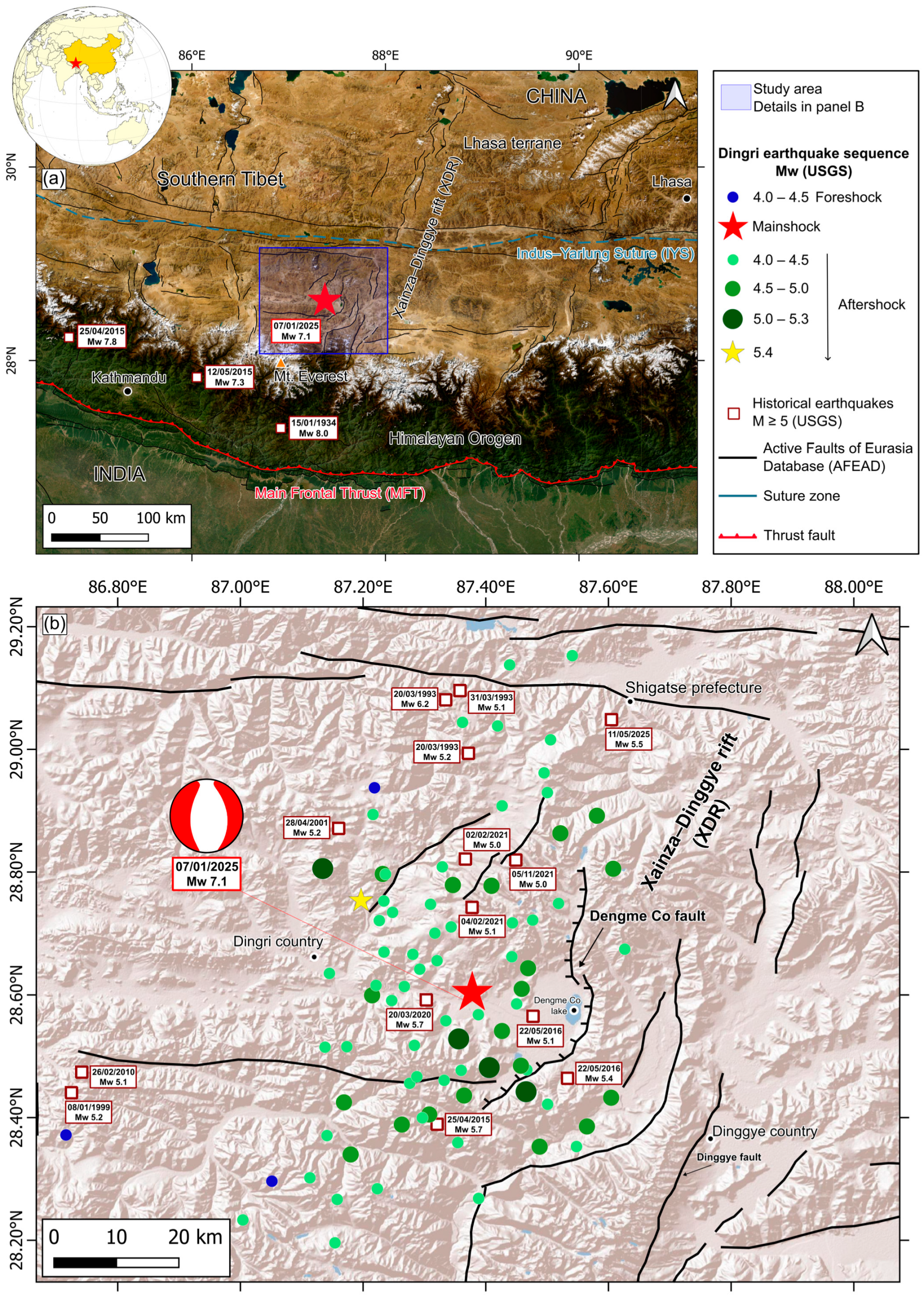
On 7 January 2025 (01:05 UTC), a Mw 7.1 earthquake struck the Southern Tibetan Plateau (Xizang) (28.573°N, 87.375°E) in the Tibet Autonomous Region of China. The event affected Dingri County, located in the southern part of the Shigatse Prefecture, reaching a maximum intensity of degree IX on the China Seismic Intensity Scale in the epicentral area (Figure 1). The earthquake resulted in at least 126 fatalities and 337 injuries, affecting approximately 60,000 people and damaging more than 27,000 buildings (about 3600 homes destroyed). The epicenter is located in the southern sector of the Tibetan Plateau, within the Lhasa Block and, specifically, in the southern portion of the north–south trending Xainza–Dinggye rift (XDR) [1].

The seismogenic fault responsible for the event is the Dengme Co Fault [1,2], a tectonic structure approximately 60 km long, characterized by a maximum slip rate of 0.5–1.0 mm/yr and associated with the system of normal faults that bounds the western margin of the Xainza–Dinggye rift (XDR) [3,4,5] (Figure 1). The focal mechanism solutions indicate that the rupture occurred along a normal fault, roughly north–south striking and dipping to the west, which propagated for about 30 s along the northern segment [1,6]. Furthermore, assuming a surface rupture zone about 25 km long, field surveys and remote-sensing data identified significant surface deformation, characterized by vertical offsets along the main fault trace, with displacements up to 3 m [2,5,7].

The mainshock, which occurred at a depth of about 10 km, was preceded by three foreshocks: two on 28 December 2024, with Mw 4.2 and 4.0 (06:05 and 7:02 UTC at a depth of 10 km) and one on 7 January 2025 (00:11 UTC at a depth of 10 km) with Mw 4.2. Furthermore, ten aftershocks with Mw > 5 have been registered in the epicentral area at a depth of about 10 km. The largest one (Mw 5.4) occurred on 7 January at 01:09 UTC, less than 30 km from the epicenter (Figure 1b).

The mainshock area is near the Indo-Eurasian plate boundary in the southern Tibetan and Himalayan regions. This area has a long history of strong earthquakes. Before this earthquake, the southern Xainza–Dinggye rift (XDR) recorded six M ≥ 5 earthquakes, including the Mw 5.7 event in 2015, two Mw 5.4 and 5.1 events in 2016, the Mw 5.7 event in 2020 and two Mw 5.0 and 5.1 events in 2021 [8] (Figure 1b). However, the Mw 7.1 Dingri earthquake on 7 January 2025, represented the culmination of the seismic sequence and the largest earthquake in southern Tibet in decades [2]. Furthermore, four months after the 2025 mainshock, a Mw 5.5 earthquake occurred about 25 km south of the Dingri epicenter [9]. In the last century, numerous high-magnitude events (>M6) occurred within 250 km of the Mw 7.1 Xizang earthquake. The most relevant ones, caused by the northward compression along thrust faults, are the M 8.0 earthquake of 15 January 1934, located about 160 km S-SE [10], and the Mw 7.8 2015 Gorkha earthquake sequence, located about 160 km to SW, which occurred on 25 April 2015, and was followed by a Mw 7.3 aftershock on 12 May 2015 [11] (Figure 1a). These latter earthquakes resulted in over 8500 fatalities, approximately 19,000 injuries, and extensive damage to public and private infrastructures, including cultural heritage sites. The relatively severe damage observed in the epicentral area is primarily attributable to structural collapses induced by strong ground shaking, which was amplified by the event’s high magnitude and very shallow hypocentral depth. Additionally, the presence of incoherent, mechanically weak lacustrine deposits in inhabited areas near active faults further amplified seismic waves, thereby increasing the destructive effects.

Previous studies carried out on the Dingri earthquake have exploited geodetic observations to derive different rupture scenarios, reflecting the inherent difficulty in characterizing the seismogenetic source. Initial analyses by [12,13] already pointed toward a complex structural framework, identifying a west-dipping primary normal fault plane coupled with a conjugate fault. Conversely, Zhao et al. [14] proposed an alternative single-plane interpretation, integrating InSAR observations with high-frequency near-field waveforms and teleseismic data to construct a three-segment fault model along the Dengme Co Fault. The hypothesis of a multi-segment involvement was also supported by [15] through the analysis of the spatial distribution of aftershock sequences. While these studies provided important insights into the understanding of the seismogenic structure, the debate between single-segment and multi-segment models persists, and the role of secondary faulting in the Dingri earthquake remains poorly constrained. The present study aims at demonstrating that the rupture was significantly more sophisticated than previously modeled. To achieve this, we combine Interferometric Synthetic Aperture Radar (InSAR) data with GNSS (Global Navigation Satellite System) observations integrated into the modeling inversion to investigate the complexity of the fault system and to constrain the geometry and slip distribution of the seismic source. Specifically, this work proposes a multi-segment rupture model over a single-segment configuration and provides robust geodetic evidence for the activation of secondary segments, including an antithetic fault. In particular, the combined dataset supports a listric geometry along the primary segment, characterized by a progressive decrease in dip with depth. Finally, the Coulomb Failure Function (ΔCFF) was derived to analyze stress transfer and accumulation on nearby active faults and to test the hypothesis of three distinct secondary segments.

Geological Setting

The southern Tibetan and Himalayan regions originated from the continental collision within a subduction context between the Indian Plate and the south margin of the Eurasian Plate about 50 million years ago (early Eocene). The N-S convergence rate is approximately 40–50 mm/yr [16]; roughly 15–22 mm/yr of this motion is accommodated by the thrust system of the Main Frontal Thrust (MFT), while the remaining deformation is heterogeneously distributed across the major north–south oriented rift systems within the plateau and along large strike–slip fault systems at its margins. This collision, the primary geodynamic driver controlling tectonic deformation, has caused crustal shortening of about 2500 km, leading to the uplift of the Himalayan Mountain range and the formation of the Qinghai–Xizang (Tibetan) Plateau, a thickening of the continental crust of about 60–70 km, and an eastward lateral translation of the Tibetan Plateau’s lithosphere along major east–west trending strike–slip faults [11] (Figure 1a).

The overall uplift of the Tibetan Plateau and the associated dynamic evolution of the landscape generated significant east–west extension (beginning in the early Miocene) and deformation within the plateau, resulting in the development of a series of large rifts composed of numerous north–south striking normal faults that bound graben or half-graben structures. The distribution of these rifts reflects the tectonic transition from the north–south compression typical of the Himalayan arc to the east–west extension observed in southern Tibet, characterized, according to previous studies, by rates of approximately 15–18 mm/y [17,18]. The structural architecture of the Xainza–Dinggye rift is influenced by the unique rheological stratification of the Southern Tibetan crust. Significant crustal thickening and a relatively shallow brittle–ductile transition [19,20] can promote the development of complex fault geometries, including depth-dependent dip variations. In particular, the N–S striking normal faults, key indicators of ongoing deformation processes, affect areas of highest seismic activity and represent the most prominent active tectonic structures of the entire Qinghai–Xizang (Tibetan) Plateau [1,9,16]. Among the numerous rift zones, the one affected by the Dingri earthquake is the Xainza–Dinggye rift (XDR), which extends at a rate of approximately 1–2 mm/yr [17,18,19] for about 350 km within the Lhasa Block (particularly in its southern sector), southward from Xainza County to Dinggye, located on the northern flank of the Himalaya, about 300 km west of Lhasa [2]. This structure cuts across more complex systems, such as the Southern Xizang Detachment System, composed of a network of low-angle strike–slip faults located in the southern part of the Qinghai–Xizang (Tibetan) Plateau, and the Indus–Yarlung Suture (IYS), which represents the collision zone between the Indian Plate and the Eurasian Plate, marking the boundary between the Lhasa Block to the north and the Himalayan range to the south. (Figure 1a). The Xainza–Dinggye Rift (XDR) system is therefore divided into three main segments (Figure 1b): the northern and southern segments are characterized by southeast-dipping normal faults, whereas the central segment comprises northwest-dipping normal faults [21]. Moreover, the Quaternary morphology of the rift is remarkable, featuring vertically displaced river terraces, alluvial fans, and moraines [2]. Specifically, in the southern part of this rift lies the Dengme Co graben, where the Dingri earthquake occurred following the activation of the Dengme Co Fault, a Holocene-active normal fault that marks the eastern boundary of the graben [4,22].

Post-earthquake field studies [2] at Dengme Co revealed coseismic vertical displacements up to 0.9 m and a long-term slip rate of 1.1 mm/yr over the past ~20 ka, implying an average recurrence interval of ~800 years. Despite its modest length (~20 km), the Dengme Co fault accommodates about 12% of southern Tibet’s total east–west extension. This highlights potential risk from other normal faults in the region (e.g., Dinggye fault), many of which lack historical earthquake records and may be approaching rupture, emphasizing the need for a thorough seismic hazard assessment of the southern Tibetan rift [2].

Figure 1. Tectonic and seismological setting of the study area. (a) Geographical setting and historical seismicity of the Xizang area, including the Indus–Yarlung Suture (IYS) and the Main Frontal Thrust (MFT). Historical seismicity (M ≥ 5.0) is indicated by white squares. The blue box outlines the area detailed in panel (b). (b) Local seismotectonic map of the Dingri region. The focal mechanism of the mainshock is shown jointly with the foreshocks (blue circles) and aftershocks (green circles), which are scaled by magnitude [23]. The active faults from the Active Faults of Eurasia Database (AFEAD) [24].

Figure 1. Tectonic and seismological setting of the study area. (a) Geographical setting and historical seismicity of the Xizang area, including the Indus–Yarlung Suture (IYS) and the Main Frontal Thrust (MFT). Historical seismicity (M ≥ 5.0) is indicated by white squares. The blue box outlines the area detailed in panel (b). (b) Local seismotectonic map of the Dingri region. The focal mechanism of the mainshock is shown jointly with the foreshocks (blue circles) and aftershocks (green circles), which are scaled by magnitude [23]. The active faults from the Active Faults of Eurasia Database (AFEAD) [24].

2. Materials and Methods

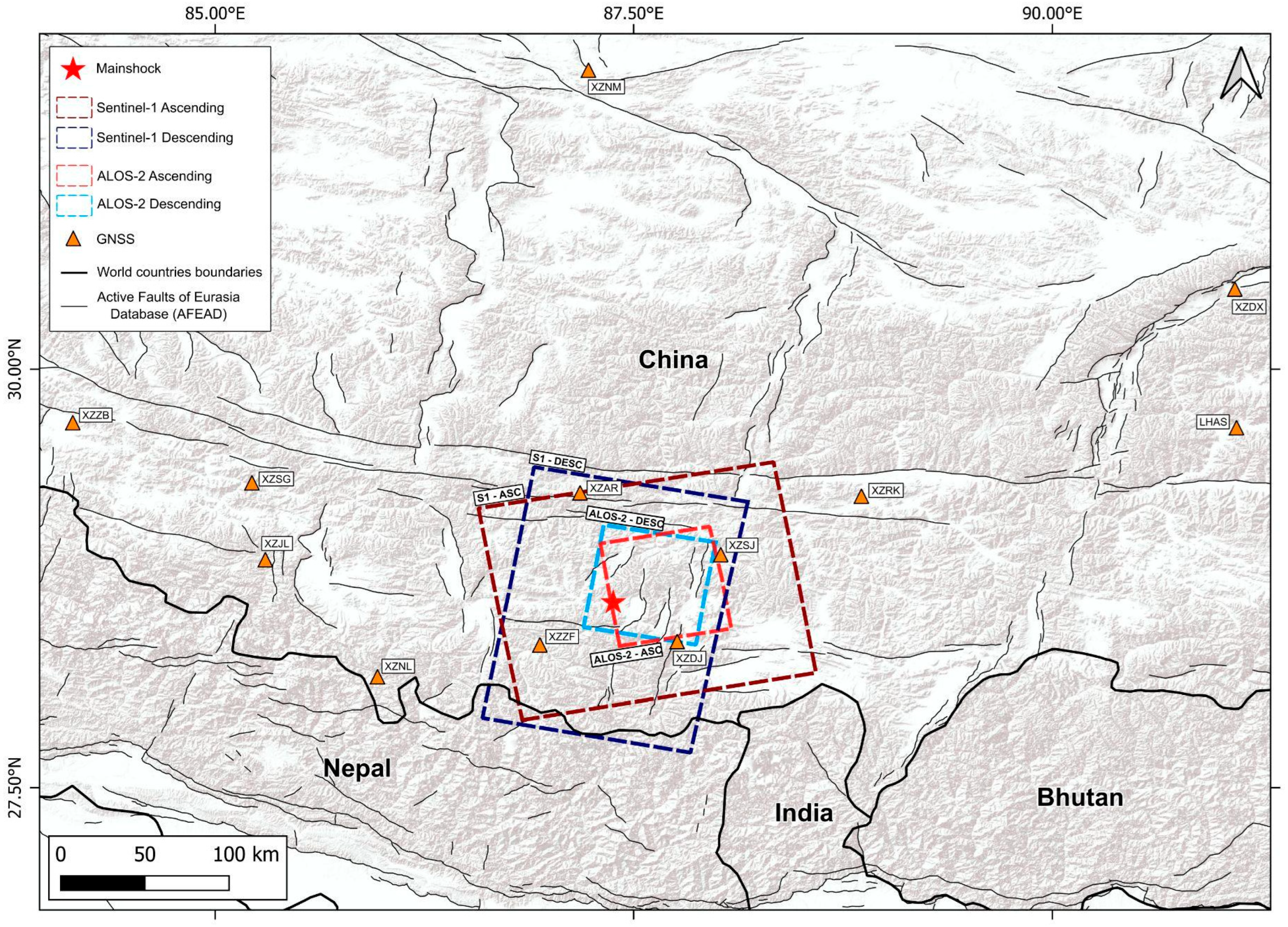
In this study, C-band Single-Look Complex (SLC) Sentinel-1 data acquired in TOPSAR mode from the European Space Agency (ESA), together with L-band ALOS-2/PALSAR-2 data acquired in Stripmap mode from the Japan Aerospace Exploration Agency (JAXA), were employed to measure the coseismic ground displacement associated with the Mw 7.1 Dingri earthquake. Notably, although L-band data may be affected by ionospheric delays, they are generally less affected by temporal and geometric decorrelation, leading to improved spatial coverage, enhanced fringe definition, and a reduced likelihood of cycle phase jumps during the phase unwrapping process. For this reason, the L-band data were incorporated into the analysis to enhance the estimation of the deformation field—particularly in the near-fault zone, where strong deformation gradients can cause significant decorrelation—and to constrain the parameters of the seismic source as well as to improve the robustness of the slip distribution retrieved during source modeling. Sentinel-1 and ALOS-2 SAR image pairs encompassing the seismic event were acquired in both ascending and descending orbits (see Figure 2 and

Table 1. Characteristics of the InSAR interferometric pairs used in this study.

Dataset	Orbit Pass	Track	Interferogram Pair	Incidence Angle (°)	Perpendicular Baseline (m)
Sentinel-1	Ascending	12	5 January 2025 17 January 2025	41	52.6
Sentinel-1	Descending	121	1 January 2025 13 January 2025	35.8	15.5
ALOS-2	Ascending	156	23 December 2024 3 February 2025	40.5	161.2
ALOS-2	Descending	47	15 October 2024 7 January 2025	40.5	68.7

) and processed using the InSAR technique [25].

The source modeling was subsequently performed by inverting the coseismic displacement fields obtained from the InSAR processing of both the Sentinel-1 and ALOS-2 datasets, jointly with the static coseismic horizontal components resulting from 12 GNSS stations within 400 km of the epicenter reported in [26] and shown in

Table 2. Observed coseismic horizontal displacements recorded by the GNSS network of the Mw 7.1 Dingri earthquake. East–West and North–South displacement components are reported with their associated uncertainties. GNSS data are sourced from [26].

Site	Longitude (°)	Latitude (°)	Epicenter Distance (km)	E-W Displacement (mm)	N-S Displacement (mm)
LHAS	91.10	29.65	377.66	2.5 ± 1.6	2.6 ± 1.4
XZAR	87.18	29.26	89.27	−8.8 ± 1.5	−0.8 ± 1.3
XZZB	84.15	29.68	345.87	−1.6 ± 1.6	1.7 ± 1.4
XZZF	86.94	28.35	52.24	−41.2 ± 1.8	−14.0 ± 1.6
XZNM	87.23	31.79	367.18	0.1 ± 1.7	1.3 ± 1.5
XZRK	88.86	29.24	160.95	10.4 ± 1.4	5.4 ± 1.2
XZDX	91.09	30.48	417.05	1.6 ± 1.6	2.0 ± 1.4
XZDJ	87.76	28.37	33.72	42.8 ± 4.1	−1.3 ± 3.3
XZJL	85.30	28.86	213.42	−5.8 ± 2.2	2.3 ± 1.9
XZNL	85.97	28.16	149.29	−10.7 ± 3.7	−0.9 ± 2.9
XZSG	85.22	29.32	234.82	−2.7 ± 2.7	2.1 ± 2.3
XZSJ	88.02	28.89	70.69	92.4 ± 3.8	25.7 ± 3.2

.

2.1. InSAR Data Analysis

InSAR provides millimetric precision in detecting ground deformation, making it a valuable tool for identifying the areas most affected by an earthquake and estimating associated surface displacements. In this study, SAR images acquired along both ascending and descending orbits were processed to quantify surface displacements caused by the Dingri earthquake in the Line of Sight (LoS) direction, defined as the line connecting the pixel on the ground to the satellite [27]. The interferograms were generated using SARscape software version 6.1 developed by sarmap SA, which is included in the ENVI package (NV5). In the first step, the 30 m ALOS World3D Digital Elevation Model released by JAXA [28] was used to assist SAR image coregistration and terrain phase elimination. The interferometric phase noise was reduced during the InSAR data processing; the multilook ratio of the interferogram was set to 4:1 and 2:4 (range:azimuth) for Sentinel-1 and ALOS-2 data, respectively. The obtained interferograms were filtered using the Goldstein filter algorithm to reduce the phase noise [29]. A window size of 64 × 64 pixels and an adaptive alpha parameter ranging from 0.3 to 2.5 were adopted, resulting in improved interferometric coherence. In fact, in order to optimize the filter performance, the alpha parameter, which characterizes the strength of the filter, is handled in an adaptive way on the basis of the local scene coherence: the lower the coherence, the stronger the filter. This filtering approach significantly improves fringe visibility and reduces the noise introduced by temporal or baseline-related decorrelation: incoherent areas are filtered more than coherent zones. This implies a signal loss minimization, while strongly reducing the level of noise. At this stage, no atmospheric delay correction was applied during the interferometric pairs generation. The following step was the phase unwrapping, where the Minimum Cost Flow was applied to remove the residual orbital phase from the interferogram using a quadratic polynomial fitting [30]. This is a robust, global optimization method for phase unwrapping, addressing the phase unwrapping problem by reformulating it as a minimum cost flow network, which effectively solves for the optimal unwrapped phase, particularly in or near highly noise-sensitive or discontinuous areas. The coherence threshold for the unwrapping operation was set to 0.3 for both the Sentinel-1 and ALOS-2 coseismic pairs production.

Finally, the ALOS World3D DEM was used to geocode both Sentinel-1 and ALOS-2 data at a spatial resolution of 15 m at the ground.

2.2. Source Modeling

To illuminate the complexity of the fault-dislocation system responsible for the observed displacement pattern, we jointly inverted InSAR and GNSS displacement data, opportunely weighted, as described later in this section. As a predictive model, we used the analytical solutions proposed by [31], which describe the surface displacement induced by a finite dislocation source in an isotropic and homogeneous medium, modified to include local topography in the calculations as described in [32].

Both the ascending and descending Sentinel-1 and ALOS-2 displacement maps were previously sampled to reduce the number of points to manage in the modeling process; sampling was performed over a regular grid with a resolution of 150 m in areas with the highest displacement rates (near field), 1000 m in regions with lower displacement rates (far field), and 5000 m at greater distances. The near-field region comprises the four aforementioned areas, each exhibiting distinct displacement patterns that we associate with four seismic fault segments. Through the sampling process, four datasets were generated, consisting of 43,771 and 43,381 points for the ascending and descending orbits of Sentinel-1, and 35,309 and 37,104 points for the ascending and descending orbits of ALOS-2, respectively.

The modeling to obtain the slip distribution follows the typical two-step approach. In the first phase, the non-linear parameters of a uniform dislocation model in an elastic half-space [31] are constrained. This inversion is applied to constrain the fault geometry under the assumption of uniform slip and is carried out using the Levenberg–Marquardt algorithm [33] to locate the global minimum, with multiple restarts incorporated to reduce the likelihood of convergence on local minima. After the best-fit parameters are obtained, their uncertainties are assessed by perturbing each dataset with spatially correlated noise and repeating the non-linear inversion as described by [34,35]. The best-fit parameters obtained through the non-linear inversion are shown in

Table 3. Best-fit values for each source model after the non-linear inversion. Their 1-sigma uncertainties are reported within brackets.

	length [km]	width [km]	depth [km]	dip [deg]	strike [deg]	east [deg]	north [deg]	rake [deg]	slip [m]
main segment (up)	20.9 (0.1)	3.4 (0.1)	−5.22 * (0.01)	70 (0.28)	184.59 (0.04)	87.5590 (0.0002)	28.7504 (0.0004)	−70.5 (0.9)	2.71 (0.03)
main segment (low)	24.7 (0.2)	11.2 (0.1)	−4.21 * (0.01)	47 (0.28)	184.59 (0.04)	87.5249 (0.0004)	28.7640 (0.0003)	−70.5 (0.9)	3.36 (0.04)
antithetic segment	10.5 (0.3)	6.5 (0.4)	−3.5 * (0.1)	50.2 (2.3)	359.7 (1.1)	87.378 (0.002)	28.748 (0.002)	−90.0 (5.5)	0.73 (0.04)
northern segment	8.5 (0.4)	5.0 (0.9)	−3.4 * (0.3)	60 (2.5)	211.6 (1.7)	87.486 (0.003)	28.928 (0.003)	−30.9 (2.5)	1.74 (0.34)
southern segment	19.2 (1.6)	6.2 (0.9)	0.9 (0.4)	53.1 (2.6)	166.4 (2.3)	87.468 (0.003)	28.535 (0.008)	−86.2 (7.6)	1.20 (0.15)

* negative values correspond to depth above the sea level.

along with their uncertainties.

The inversion process follows the approach described in Section 2 of [36] to assign the weights to the individual InSAR and GNSS datasets reported in

Table 4. Summary of selected parameters of each dataset used in the inversion: orbital direction (ascending/descending), number of inverted samples and the parameter for dataset weighting, identified through the algorithm published in [36].

Dataset	Orbit Pass	Samples (Points)	Weight
Sentinel-1	Ascending	43,771	0.020
Sentinel-1	Descending	43,381	0.028
ALOS-2	Ascending	35,309	0.007
ALOS-2	Descending	37,104	0.018
GNSS		12	0.126

. It is an iterative algorithm that exploits the properties of the chi-square statistic and converts the expansion or contraction coefficients of the nominal sigma, initially assigned to each dataset, into weights. For a detailed analytical description of the algorithm, the reader is referred to the cited literature.

Once the non-linear parameters (dimension, location, orientation, rupture mechanism and average slip) have been determined, the individual sources are extended and subdivided into 1 km patches to accommodate the slip distribution obtained through linear inversion. In this case as well, the InSAR and GNSS datasets are inverted simultaneously, adopting the weights previously determined with the non-linear inversion. During the linear inversion stage, the rake angle was fixed to the optimal value estimated for each segment during the preliminary non-linear inversion, while only the slip values were allowed to vary between patches. The inversion is performed by introducing a regularization operator to prevent unrealistic slip fluctuations, appropriately weighted by a damping factor. An additional constraint is imposed through the use of the BVLS (Bounded-Values Least Squares) algorithm, which a priori prevents negative slip values (back-slip). Further details with a formal description of the Green’s matrix setup can be found in [37]. For completeness, we note that both in the non-linear and linear inversion stages, parameters describing possible offsets and orbital ramps affecting the various InSAR datasets are jointly estimated together with the source model parameters.

2.3. Coulomb Failure Function (CFF) Analysis

Variations in static stress (ΔCFF) induced by natural events may influence the timing of subsequent earthquakes [38]. To investigate whether the main segment could have triggered the activation of the antithetic, northern, and southern segments, we calculated the static ΔCFF. Coulomb stress changes were computed according to

ΔCFF = Δτ + μ′Δσ

where μ′ = μ (1 − β) is the effective friction coefficient, μ is the coefficient of friction, and β is the Skempton parameter [39,40]. Here, Δτ denotes the shear stress change, while Δσ represents the normal stress change, taken as positive for extensional stress. An apparent friction coefficient of 0.4 was adopted. We computed the six components of the induced stress tensor and subsequently derived the corresponding changes in normal, shear, and Coulomb stress.

3. Results

3.1. InSAR Displacement Maps

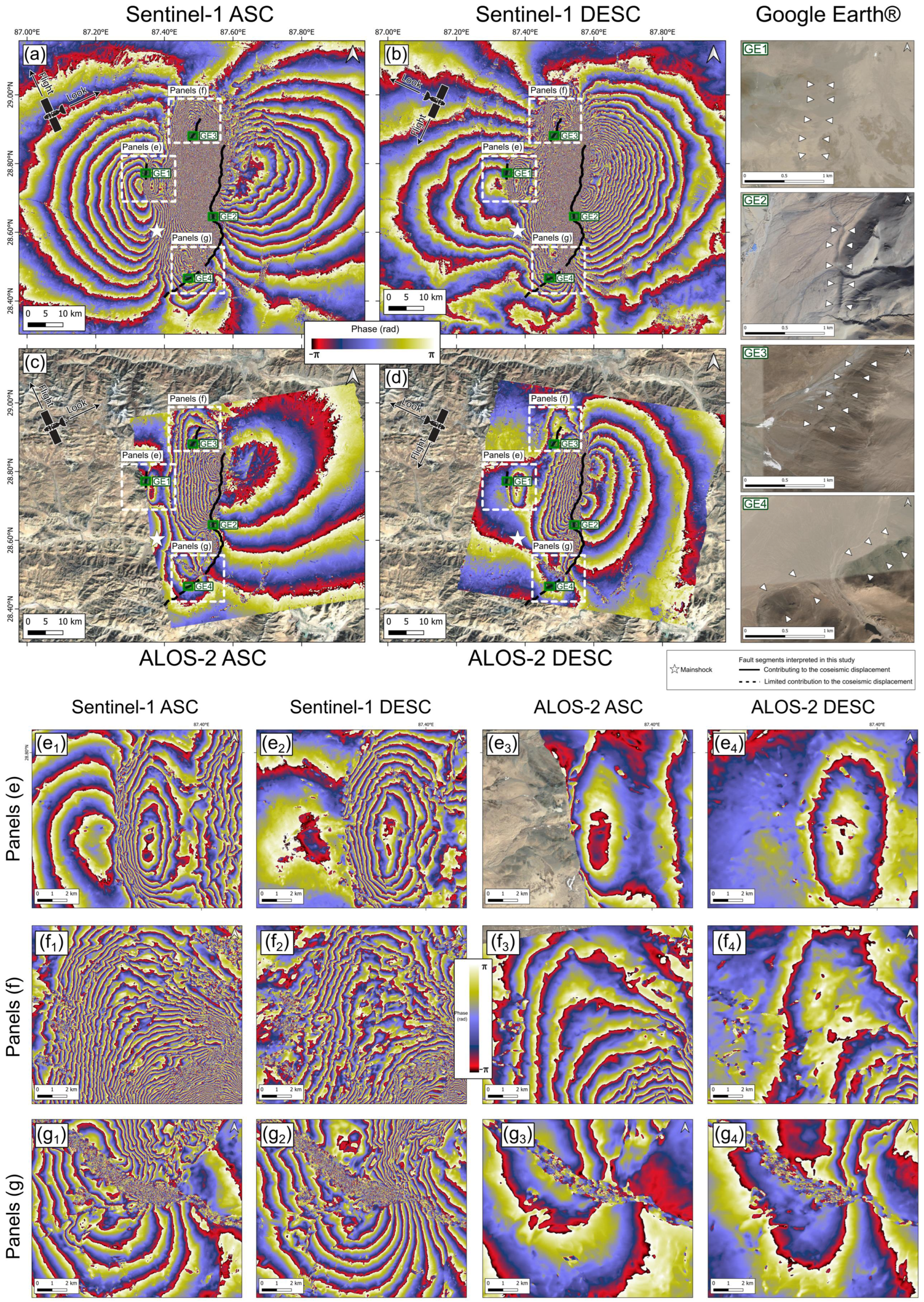
The four coseismic wrapped interferograms computed for the Sentinel-1 ascending (Figure 3a) and descending (Figure 3b) orbits, as well as for ALOS-2 ascending (Figure 3c) and descending (Figure 3d) orbits, exhibit a complex pattern characterized by four main, spatially distinct deformation areas (see zoomed panels in Figure 3). Differences in the deformation patterns are observed between the Sentinel-1 and ALOS-2 interferograms. These discrepancies can be attributed to the different radar wavelengths and acquisition characteristics of the two sensors. In particular, the L-band ALOS-2 data (λ ≈ 23 cm) generally are less affected by temporal and geometric decorrelations and phase unwrapping errors, thus enhancing the estimation of the deformation field. In contrast, the C-band Sentinel-1 data (λ ≈ 5.6 cm) are more sensitive to decorrelation effects. As a result, variations in fringe continuity and phase gradients may arise, especially in near-field areas where deformation is more localized and complex. Despite these local differences, the overall deformation patterns remain consistent between the datasets.

Among the four identified displacement patterns, the principal and largest, elongated in a north–south direction, is located in proximity to the main and well-known Dengme Co Fault. Three additional local displacement patterns of minor amplitude are identified to the west (panel e in Figure 3), north (panel f in Figure 3), and south (panel g in Figure 3) of the principal deformation area, as indicated by concentric fringe patterns. Photogeological interpretation of Google Earth digital orthophotos carried out in this study (see panels GE1–GE4 in Figure 3), combined with comparison to previously published studies [2,4,12], suggests the presence of pre-existing faults in those areas exhibiting localized deformation patterns. Possible pre-existing structures inferred in this study through photogeological analysis along the Dengme Co fault, as well as in the northern and western areas, are indicated by solid and dashed lines in Figure 3. In contrast, no clear counterpart structures for the southern deformation area are reported in the existing literature, which may indicate either the activation of previously unmapped structures or limitations in the current geological datasets. In Figure 3, the main segment mapped in this study corresponding to the Dengme Co fault is represented by a solid and dashed line, corresponding respectively to a clearly identifiable northern portion (GE2 in Figure 3) and a less distinct southern portion of the fault trace (GE4 in Figure 3), respectively. The northern portion of the main segment appears to have contributed more significantly to coseismic deformation, whereas the southern portion shows a more subdued expression. This evidence provides insight into the complexity of the fault system activated during the earthquake and suggests the possible involvement and reactivation of older tectonic structures.

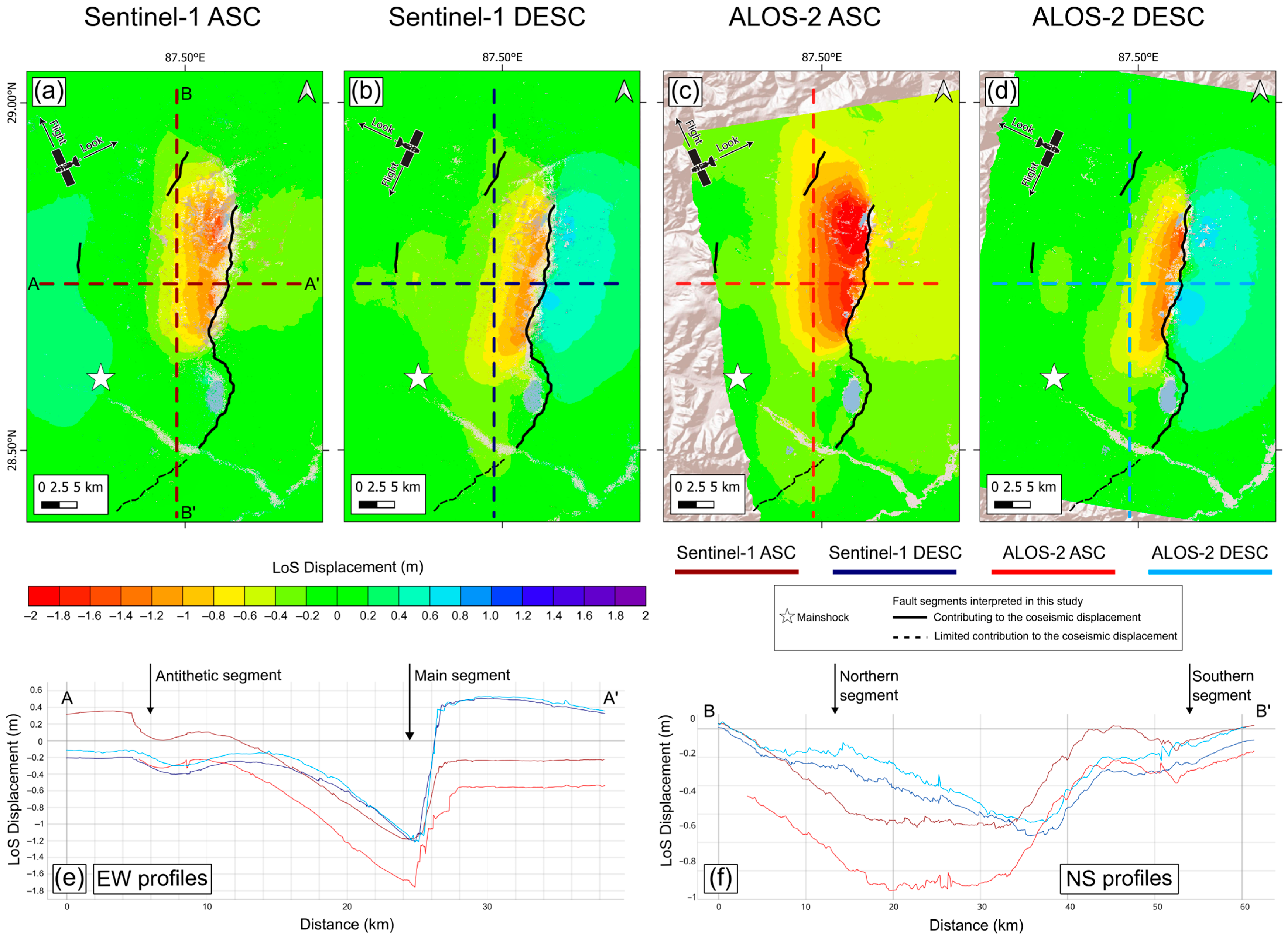
The Sentinel-1 (Figure 4a,b) and ALOS-2 (Figure 4c,d) coseismic LoS displacement maps, exhibiting values from −2 to 2 m across both ascending and descending orbits, indicate a clear pattern compatible with the dislocation of the northern portion of the main segment identified by photogeological analysis (solid black line in Figure 4a–d). This sector is characterized by a high density of fringes (Figure 3) and sharp displacement gradients, indicative of significant near-field deformation. In contrast, the southernmost portion of this main segment (dashed black line in Figure 4a–d) shows limited contribution to the observed coseismic deformation, as confirmed by patterns in the wrapped interferograms in Figure 3a–d. Secondary deformation signals are observed in correspondence with the northern, western and southern areas, although with lower amplitudes compared to the main segment. In particular, the deformation pattern identified in the western area is interpreted as an antithetic segment dipping opposite to the main fault. These features suggest the involvement of secondary structures in the rupture process, although with relatively minor displacement contributions. The coseismic deformation is further illustrated by the A–A′ and B–B′ displacement profiles shown in Figure 4. Along profile A–A′, both the main and antithetic segments exhibit consistent displacement patterns across the two satellite datasets, with displacements of up to ~0.2 m (descending) and ~0.4 m (ascending) for the antithetic segment, and up to ~1.4 m (descending) and ~1.0 m (ascending) for the main segment. Along profile B–B′, pronounced displacement is observed across the main segment (up to ~0.6 m for both orbits), accompanied by minor deformation associated with the northern and southern segments. Overall, the observed displacement field reflects a highly complex rupture geometry, likely involving the activation of at least four distinct fault segments characterized by differing lengths, orientations, and dip angles.

3.2. Source Modeling and ΔCFF Analysis

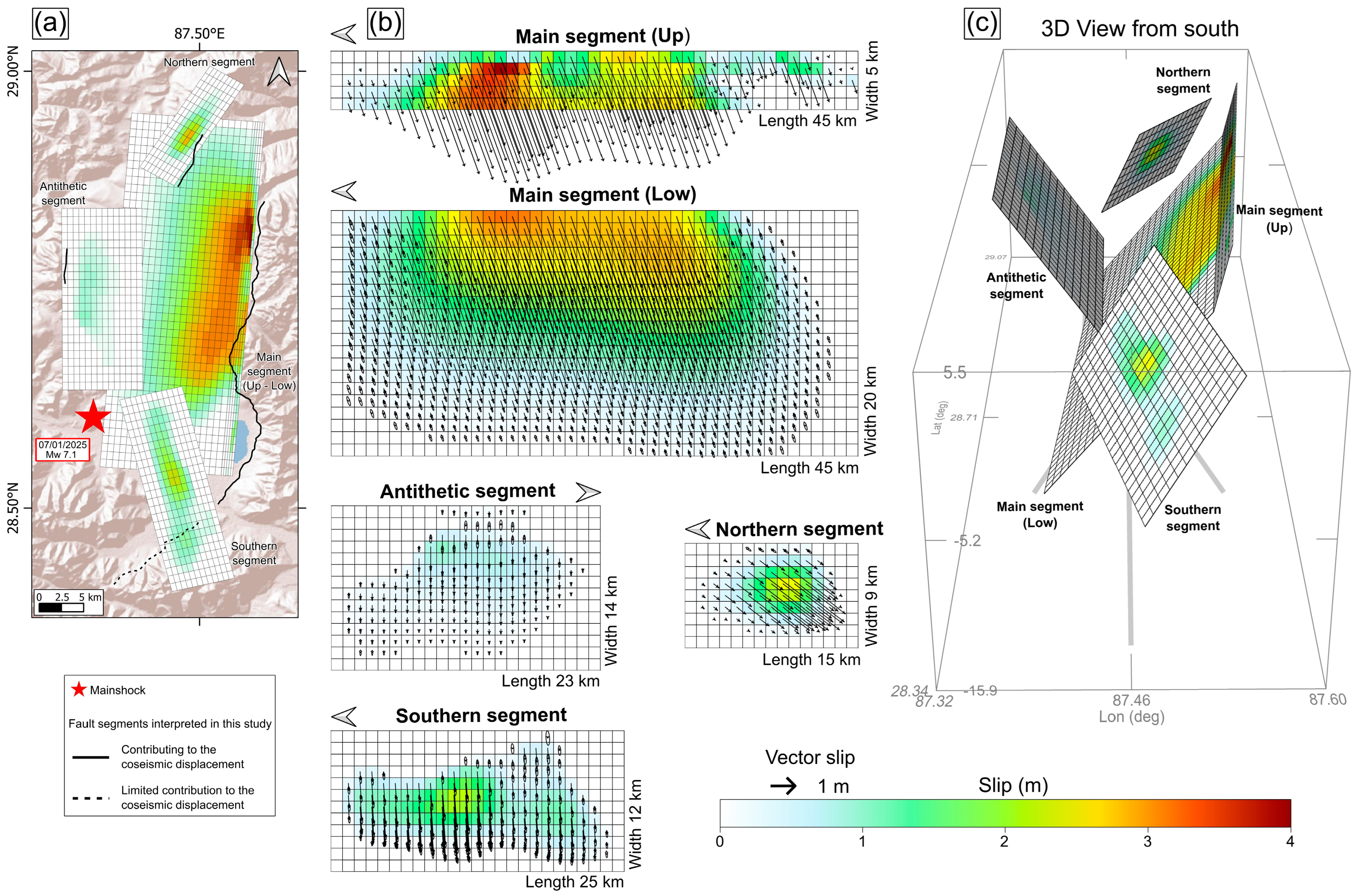
As mentioned in Section 2.2, the modeling was carried out considering the deformation patterns visible in the displacement maps (Figure 4a–d) and the GNSS coseismic horizontal displacements. The resulting model (Figure 5) consists of one primary segment (along the Dengme Co Fault) and three secondary segments. The main segment, modeled as a listric fault, is oriented approximately north–south and dipping westward (strike 185°, and a dip of 75° and 47° for upper and lower segments, respectively).

The secondary segments include an antithetic segment also oriented north–south dipping eastward (strike 359°, dip 50°), a segment located in the north of the main one (strike 212°, dip 60°), and a segment located in the south of the main one, both with an orientation close to that of the main segment (strike 166°, dip 53°).

All four segments exhibit a predominantly normal rupture mechanism (

Table 5. Main rupture parameters derived from the inversion of InSAR data for each modeled segment and the overall rupture. In the right column, the focal mechanisms corresponding to the four segments and the overall rupture are shown, indicating the presence of a non-double-couple component. In the last row, for comparison, the parameters and the focal mechanism calculated by the USGS [6] are reported.

Segment	Strike (deg)	Dip (deg)	Rake (deg)	Seismic Moment (N*m)	Magnitude (Mw)	Focal Mechanism
main	185	61 *1	−70	4.02 × 1019	7.0
antithetic	359	50	−90	1.65 × 1018	6.1
northern	212	60	−31	1.86 × 1018	6.1
southern	166	53	−86	4.93 × 1018	6.4
TOTAL (this paper)	183 *2	60 *2	−72 *2	4.76 × 1019	7.1
USGS	187	49	−78	4.75 × 1019	7.1

*¹ average of the upper and lower dip angles. *² values are weighted averages of the parameters of the segments along the Dengme Co Fault (i.e., the main and southern segments), with weights proportional to the seismic moment.

), although the variable rake slip distribution on the main segment shows a minor left-lateral component. The comparison with the focal mechanism derived from the moment tensor by USGS [6], with strike 187°, dip 49°, rake −78°, shows significant similarity with the values of the main segment modeled from the InSAR data, including the slight deviation from a purely double-couple shown in the focal mechanism (Table 5). The choice of a westward-dipping primary fault—consistent with Plane 2 of the USGS solution [6]—is constrained by joint interpretation of the observed LoS InSAR displacement field and the USGS focal mechanism, which together resolve the inherent nodal plane ambiguity of double-couple sources. This westward-dipping geometry is also structurally consistent with the regional tectonic regime of the Xainza–Dinggye rift and mapped surface traces. Furthermore, the USGS seismological data deviates from a pure double-couple solution (approximately 89%), suggesting non-coplanar rupture processes that could align with the source complexity proposed in this study.

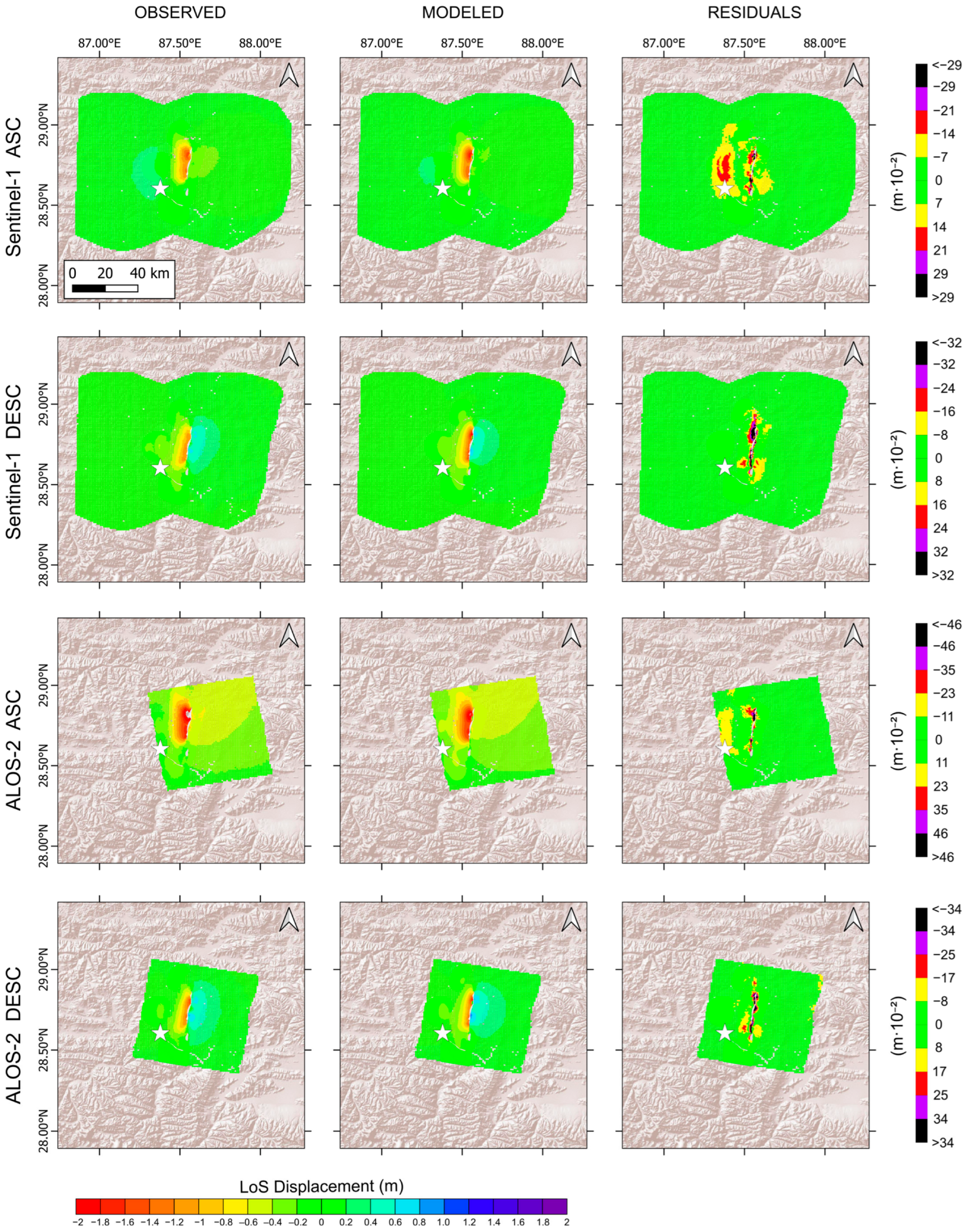
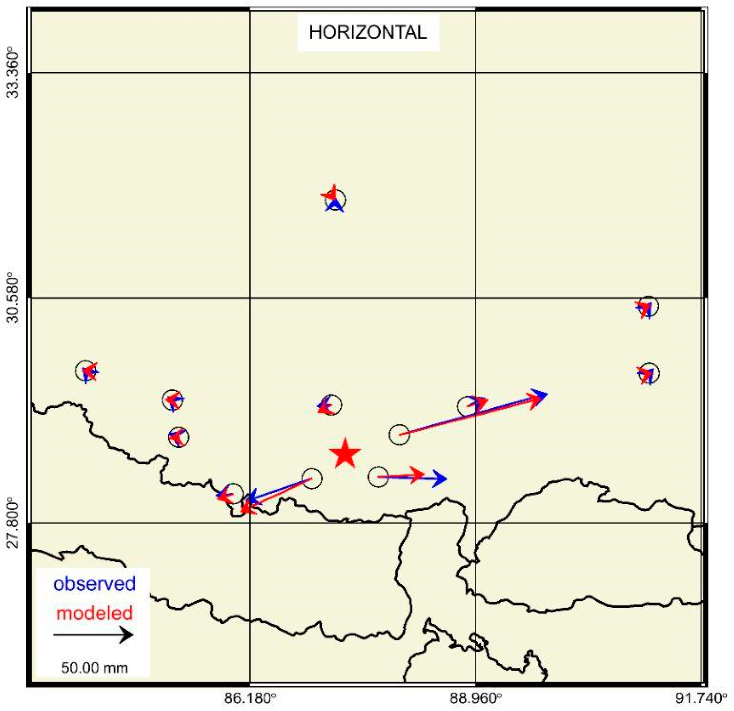
Regarding the rupture distribution, the slip on the upper portion of the main segment interests an area of approximately 45 × 5 km, with a peak of 4 m, with non-zero values reaching the local topography, whereas the lower portion of the main segment interests an area of approximately 45 × 20 km, with a peak of 3.5 m (Figure 5). A left-lateral slip component is also consistent with the slip distribution calculated by USGS through seismological inversion of P- and SH-waveforms [41]. The slip and rake values for the shallowest patches in the upper portion of the main segment may be less reliable due to high fringe density, particularly in the Sentinel-1 interferograms, which could have introduced unwrapping errors. Nevertheless, the overall uncertainty pattern indicates that the model is generally well constrained. The shape and orientation of the uncertainty ellipses in Figure 5 indicate that the model resolution is anisotropic, with greater uncertainty along specific directions. This reflects the intrinsic limitations of InSAR LoS measurements, which constrain deformation more effectively in certain geometrical directions than others. In terms of model resolution, lower uncertainties are observed in the near-field region, close to the fault trace, where deformation gradients are higher and better constrained by the InSAR and GNSS datasets. In these areas, the fault patches are more reliably resolved, resulting in a more robust estimation of slip distribution. Conversely, uncertainties tend to increase with distance from the fault and at greater depths, where the deformation signal becomes smoother and less sensitive to small-scale variations in fault geometry and slip. This reflects a common limitation in geodetic inversions. The other three segments exhibit slip that does not reach the surface, with a peak of approximately 1.1 m for the antithetic segment, 2.7 m for the northern segment, and 2.4 m for the southern segment (Figure 5). The secondary fault segments are generally characterized by relatively low and quite homogeneous uncertainties, suggesting a reasonable constraint on their slip distribution. However, the southern segment shows a moderate increase in uncertainty at depth, which may be related to the reduced sensitivity of the data to deeper slip and the lower amplitude of the deformation signal in this area. The robustness of the dislocation model obtained from the inversion of InSAR data is demonstrated by comparing the observed and modeled data (Figure 6). The modeled displacement fields reproduce the main spatial features of the observed deformation patterns for both Sentinel-1 and ALOS-2 data. In particular, the model successfully replicates the primary deformation associated with the main fault segment, as well as the secondary segments. The residual maps are generally characterized by low-amplitude, spatially scattered signals, indicating a good agreement between observations and model predictions. Residuals are slightly higher in the near-field areas, as well as in correspondence with secondary segments, suggesting minor mismatches likely related to local complexities in fault geometry and slip distribution, as well as limitations of the InSAR data, particularly in areas affected by decorrelation or strong and complex deformation gradients. In Figure 7, the observed and modeled GNSS horizontal displacements show a good overall agreement, with the model successfully replicating both the magnitude and direction of the measured vectors. This indicates that the model reproduces both the InSAR deformation field and the GNSS displacement vectors, increasing confidence in the inferred fault geometry. The generally low residuals are quantitatively confirmed by the Root Mean Square RMS values for each dataset (Table S1, Supplementary Materials) used in the linear inversion, supporting the overall quality of the model fit.

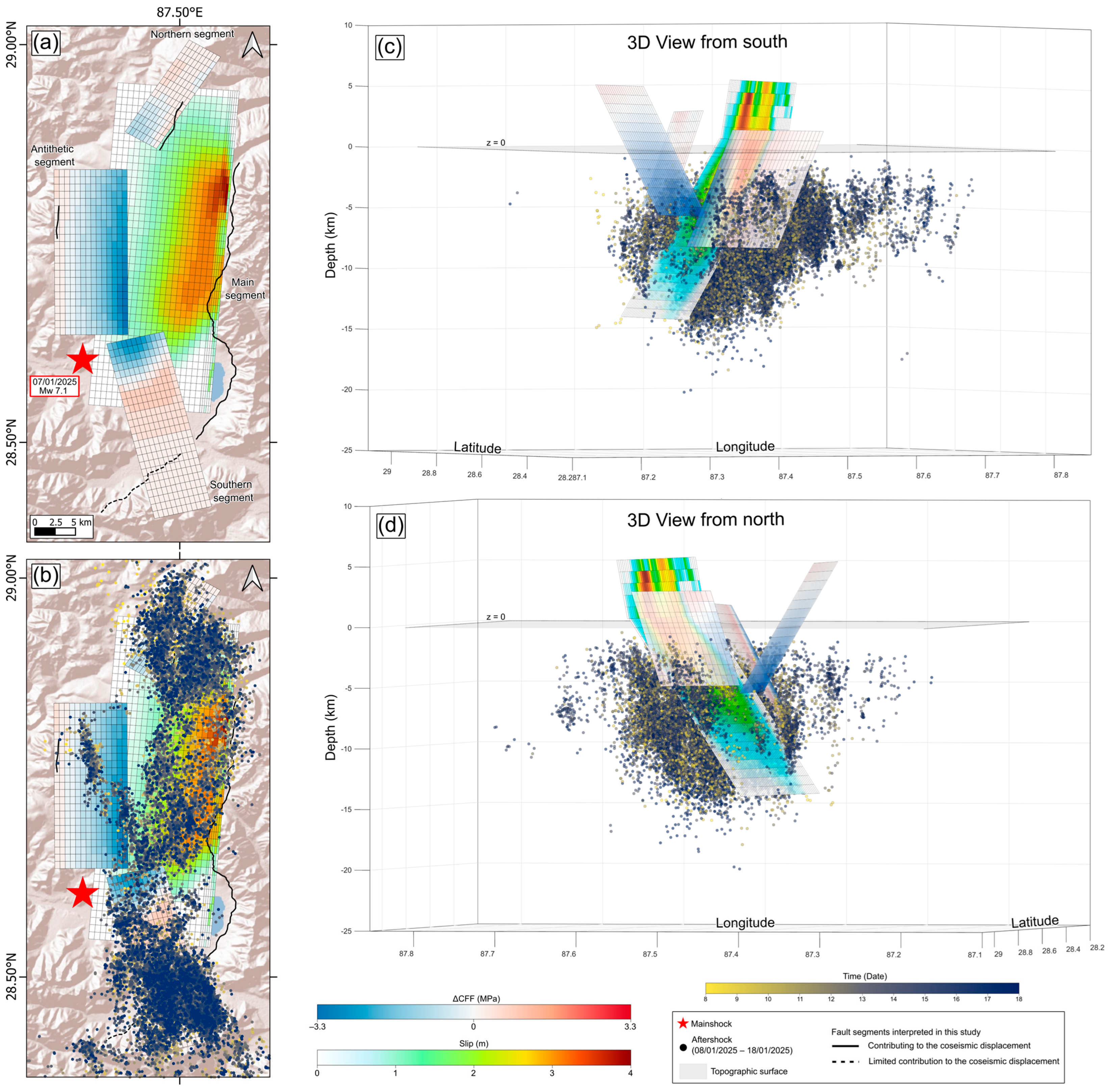
To evaluate whether the rupture of the main segment could have activated the antithetic as well as both northern and southern segments, we calculated the static stress variation (ΔCFF, Coulomb Failure Function) (Figure 8). This analysis was performed to assess whether the rupture of the main segment could have positively loaded the antithetic segment and the other two secondary segments, thus facilitating its rupture. Indeed, the ΔCFF calculation indicates that the upper part of the antithetic segment experienced a positive stress increase of approximately 0.3 MPa; the same methodology was applied to the northern and southern segments, revealing a stress increase of about 0.4 and 0.8 MPa across most of their respective areas (Figure 8a).

The spatial distribution of aftershocks collected from 8 January to 18 January by [15] shows a clear clustering along the main fault and secondary segments, with a tendency to concentrate in areas characterized by positive stress changes, especially along both northern and southern segments. This spatial correlation supports the consistency between the modeled segments, the stress changes and the observed seismicity pattern.

4. Discussion

The source modeling applied to the InSAR displacement field enables the retrieval of the geometry of the main causative faults of the coseismic deformation.

The geodetic observations (Figure 3 and Figure 4) reveal that the coseismic rupture associated with the Dingri earthquake is characterized by a high degree of structural complexity, which cannot be adequately reproduced by a single-segment planar fault model. This is evidenced by the systematic misfits observed in the residual maps (Figure S1, Supplementary Materials), particularly in areas corresponding to the secondary segments identified in this study, as well as by the higher RMS values reported in Table S1. Instead, a multi-segment fault system is required to capture the spatial variability of the deformation field. The multi-segment fault system interpretation is also consistent with [15], who identified a segmentation of aftershocks into three main clusters, supporting the presence of a structurally complex rupture. The multi-segment fault system identified in this study consists of a primary north–south-trending listric fault segment, and three secondary segments: one to the north and one to the south of the main segment, and an additional east-dipping segment located approximately 15 km to the west (Figure 4). These secondary segments play a key role in reproducing the observed spatial variability of the deformation field.

Multiple lines of evidence support the presence of these structures. In particular, the consistency of the deformation patterns observed in both Sentinel-1 and ALOS-2 datasets, despite their different radar wavelengths and sensitivity to decorrelation effects, further strengthens the interpretation that these features reflect real tectonic structures rather than artifacts related to data limitations or processing. This is further corroborated by localized fringe patterns (Figure 3), displacement gradients and profiles (Figure 4), and the spatial distribution of aftershocks. The alignment of aftershock clusters with the modeled fault segments (Figure 8) provides independent support for their involvement in the coseismic rupture process, suggesting new fault activation or reactivation of pre-existing faults within the rift system.

The analysis of static Coulomb stress changes (ΔCFF) indicates that the rupture of the main segment may have promoted failure on the adjacent secondary structures. Positive stress changes are observed on all secondary segments, suggesting that stress transfer facilitated their potential simultaneous activation. This interpretation is consistent with the spatial distribution of aftershocks, which predominantly cluster in areas of positive stress change (Figure 8). However, some events also occur in regions of negative or low stress variation, likely reflecting the structural complexity of the fault system, uncertainties in aftershock locations, and the influence of unmodeled secondary structures.

From a temporal perspective, InSAR data include 5 to 10 days of post-event deformation, during which nine events of magnitude greater than 5 occurred [42]. However, the post-seismic image of the descending ALOS-2 pair was acquired at 06:06 UTC on 7 January, just five hours after the Mw 7.1 mainshock. The descending displacement map derived from this ALOS-2 pair (Figure 3 and Figure 4) already reveals secondary deformation patterns associated with the antithetic segment as well as the northern and southern fault segments, indicating that these features developed during or immediately following the main rupture.

The seismic moment analysis of the four segments (Table 5), which together released an energy equivalent to 4.76 × 10¹⁹ Nm, further supports this observation: the antithetic segment alone released a seismic moment of 1.65 × 10¹⁸ Nm, corresponding to an M 6.1 event, significantly greater than any aftershock recorded between the mainshock and the ALOS-2 post-seismic acquisition. Similarly, the northern and southern segments released a seismic moment of 1.86 × 10¹⁸ Nm and 4.93 × 10¹⁸ Nm, respectively, equivalent to other M 6.1 and M 6.4 events, thus confirming the hypothesis that these segments almost certainly activated simultaneously with the mainshock.

Among the secondary structures, the antithetic fault segment deserves particular attention due to its clear expression in the interferometric data. It is essential to note that the presence of a source segment in an antithetic configuration does not have equally evident precedents in geodetic data from past events. In some studies, such as the 1995 Kozani–Grevena earthquake in Greece [43] or the 2016 Norcia earthquake in Italy [44], the presence of an antithetic segment was hypothesized, but without clear fringe patterns as in this case. In this latter case, the afterslip inversion model based on geodetic measurements required the activation of an antithetic fault [45]. For this reason, this circumstance warrants further investigation to corroborate the hypothesis that the antithetic segment was activated simultaneously with the mainshock, as also confirmed by the presence of morphological indicators of a fault segment compatible with the coseismic displacement field, as in Figure 3.

The multi-segment rupture model proposed in this study is consistent with the broader tectonic framework of the Southern Tibetan Plateau, where active E–W extension is accommodated by systems of interacting N–S striking normal faults within a thickened continental crust [2,46]. Elliott et al. [47] highlighting this feature of the Southern Tibetan Plateau. The involvement of conjugate multi-segment geometries in the Dingri earthquake has also been highlighted in other recent studies [12,13,19]. In this context, the InSAR observations and modeling presented in this study provide key constraints supporting multi-rupture segmentation. While normal faults in extensional settings can exhibit a range of geometries, the adoption of a listric profile in our model could provide a more physically consistent representation of the Dingri earthquake. Specifically, from a modeling perspective, the adoption of a listric geometry for the main segment is required to simultaneously reproduce both the far-field and near-field deformation patterns. A low-angle planar fault adequately fits the far-field signal (Figure S2 in the Supplementary Materials) but fails to reproduce the near-field deformation (Figure S4 in the Supplementary Materials). Conversely, a steeper-angle planar fault is needed to account for the near-field displacement, but leads to a degradation of the far-field fit. The listric geometry provides this trade-off by accommodating a progressive decrease in dip with depth (from ~70° to ~47°), consistent with extensional tectonic environments. This configuration is also compatible with the inferred shallow brittle–ductile transition in the Southern Tibetan Plateau, where fault planes tend to flatten as they approach deeper rheological discontinuities [20]. Independent geophysical observations further support this interpretation: a brittle–ductile transition zone in proximity to the main fault has been identified by [19], based on high-frequency seismic radiators and low-resistivity, low-velocity crustal anomalies (Vs < 3.2 km/s). Finally, the adoption of a listric geometry results in a measurable improvement in the model’s ability to fit the InSAR observations across all datasets, as demonstrated by the reduction in RMS values and near-field residuals compared to a planar main fault model (Table S1 and Figure S4 in the Supplementary Materials). Quantitatively, the reduction in RMS residuals from a planar to a listric main fault model ranges from 6.5% to 13.9%. Notably, the most significant improvement is observed in the ALOS-2 ascending dataset, where the RMS residual value decreases from 0.137 to 0.118 (~13.9%) and for the Sentinel-1 descending dataset, where the RMS decreases from 0.093 to 0.082 (~11.8%). More moderate but still significant improvements are obtained for Sentinel-1 ascending from 0.079 to 0.073 (~7.6%) and ALOS-2 descending from a value of 0.092 to 0.086 (~6.5%) (Table S1 in the Supplementary Materials). This differential improvement is physically consistent with the characteristics of the SAR sensors and the rupture geometry. The L-band ALOS-2 data, being less susceptible to decorrelation in areas of high displacement gradients, provides a more coherent and reliable signal in the near-field region. Consequently, the listric model is better able to reproduce these high-amplitude near-field observations. The lower percentage of improvement in the ALOS-2 descending dataset (~6.5%) suggests that, for this specific acquisition geometry, the planar approximation was already partially consistent with the LoS projection, although the listric model remains statistically superior. Overall, these results indicate that a depth-dependent dip is a necessary complexity to refinement to reduce systematic misfits and accurately reproduce the observed InSAR displacement field.

The modeled listric fault segment predicts a shallow rupture with a displacement up to 3 m (Figure 5), in agreement with the field investigations carried out by [5,7]. This consistency further supports the reliability of the proposed fault geometry and highlights the limitations of planar main fault models, which fail to reproduce both the near-field deformation and the observed surface rupture (Figure S4 in the Supplementary Materials).

As for past applications of InSAR to earthquake studies, the overall picture of coseismic displacements has contributed to accurate fault mapping and to the identification of previously recognized and unrecognized faults [48]. In this paper, the analysis of earthquake effects was conducted in a multidisciplinary and quantitative manner, leveraging state-of-the-art modeling and data interpretation techniques. In particular, through analytical modeling, stress transfer analysis, and photointerpretation, this study tests the hypothesis of the activation of three secondary segments, including an antithetic segment, during the energy release of the mainshock. Although the presence of antithetic faults is well-documented in literature and supported by seismotectonic analyses of past events, the case of the Dingri earthquake on 7 January 2025 is unique in that it demonstrates the existence and coeval (with the mainshock) activation of the antithetic segment with unprecedented clarity in the InSAR data era.

Overall, this study highlights the importance of integrating multiple geodetic and seismological datasets to constrain earthquake source models. The results provide new insights into the structural complexity of normal faulting in the Southern Tibetan Plateau, emphasizing the role of segmented and listric fault systems in accommodating crustal extension.

5. Conclusions

This study shows a refined and novel interpretation of the seismic source of the 7.1 Dingri earthquake using multi-sensor InSAR observations integrated with source inversion, stress transfer analysis, and photogeological interpretation. The results demonstrate that the observed coseismic deformation cannot be explained by a single-segment planar source, but instead requires a complex multi-segment geometry, which is consistent with the structural architecture of the Xainza–Dinggye rift.

The inverse modeling identifies a primary north–south-trending listric fault segment as the main contributor to the deformation, characterized by maximum slip values of up to approximately 4 m and shallow surface displacements of approximately 3 m. The rupture process involved the activation of three secondary segments, which are required to reproduce the displacement field: two located to the north and south of the main segment, and an east-dipping antithetic segment approximately 15 km to the west. The involvement of these secondary segments is supported by early post-event ALOS-2 observations acquired only five hours after the mainshock, inverse source modeling combined with seismic moment estimates for each segment, the Coulomb stress analysis and the spatial distribution of the aftershocks. Overall, this work demonstrates the effectiveness of an InSAR-based analysis for resolving complex rupture processes and identifying secondary segments, including an antithetic fault. The Dingri earthquake provides an evident and well-constrained example of multi-segment activation during a major normal-faulting event, with important implications for understanding fault interactions and seismic hazard in extensional tectonic settings.

References

1. Zhang, L.; Li, M.; Liu, B.; Ge, D.; Guo, Z.; Chen, Y.; Wan, X.; Wang, Y. Characterization of Co-Seismic Deformation and Geological Hazard Development of Dingri MS6.8 Earthquake in Xizang. Saf. Environ. Eng. 2025, 32, 1–13. [Google Scholar] [CrossRef]
2. Wu, K.; Chevalier, M.-L.; Pan, J.; Liu, F.; Yang, S.; Zhang, S.; Su, Q.; Li, H. Recurrence of Large Earthquakes along the Southern Xainza-Dinggye Rift and Comparison with the 7 January 2025, Mw7.1 Tingri Earthquake, Southern Tibet. Tectonophysics 2025, 910, 230827. [Google Scholar] [CrossRef]
3. An, Y.R.; Liu, Y.; Ju, H.C.; Zhang, Y.; Yu, Z.; Tang, L.; Yang, Z.; Gao, J.; Xv, L.; Li, B.; et al. Characteristics and Seismogenic Structure of the 2025 Xizang Tingri M6.8 Earthquake Sequence. Chin. J. Geophys. 2025, 68, 3713–3725. (In Chinese) [Google Scholar] [CrossRef]
4. Qiao, J.-X.; Shi, F.; Li, A.; Li, T.; Zhang, D.; Wang, X.; Gesang, D.Z.; Sun, H. Coseismic Surface Rupture of the MS6.8 Dingri Earthquake in Xizang, China, Based on GF imagery interpretation. Seismol. Geol. 2025, 47, 789. [Google Scholar] [CrossRef]
5. Xu, X.; Wang, S.; Cheng, J.; Wu, X. Shaking the Tibetan Plateau: Insights from the Mw 7.1 Dingri Earthquake and Its Implications for Active Fault Mapping and Disaster Mitigation. npj Nat. Hazards 2025, 2, 16. [Google Scholar] [CrossRef]
6. USGS. M 7.1—2025 Southern Tibetan Plateau Earthquake. Available online: https://earthquake.usgs.gov/earthquakes/eventpage/us6000pi9w/moment-tensor (accessed on 29 January 2026).
7. China Earthquake Administration. 我们在行动|地质所、四川局、西藏局联合调查团队发现定日地震的同震垂直位错量达3 m. Available online: https://mp.weixin.qq.com/s/qtB9yU9E6TlfQ4HrF5Hybw?fbclid=IwY2xjawHxy6VleHRuA2FlbQIxMAABHUdOYgqe7_OBL8rtMyQ2n5jMCqU17clFT0ex0nvadjaTabP0Cs_eHeTh8w_aem_Qt3SQrycjRENHBTY95pwPQ (accessed on 29 January 2026).
8. USGS. Latest Earthquakes. Available online: https://earthquake.usgs.gov/earthquakes/map/?extent=26.6671,83.63892&extent=30.9729,92.42798&range=search&timeZone=utc&search=%7B%22name%22:%22Search%20Results%22,%22params%22:%7B%22starttime%22:%221990-01-01%2000:00:00%22,%22endtime%22:%222025-01-30%2023:59:59%22,%22maxlatitude%22:30.06,%22minlatitude%22:27.606,%22maxlongitude%22:90.242,%22minlongitude%22:85.825,%22minmagnitude%22:5,%22orderby%22:%22time%22%7D%7D (accessed on 31 March 2026).
9. USGS. Search Earthquake Catalog. Available online: https://earthquake.usgs.gov/earthquakes/search/ (accessed on 29 January 2026).
10. Sapkota, S.N.; Bollinger, L.; Klinger, Y.; Tapponnier, P.; Gaudemer, Y.; Tiwari, D. Primary Surface Ruptures of the Great Himalayan Earthquakes in 1934 and 1255. Nat. Geosci. 2013, 6, 71–76. [Google Scholar] [CrossRef]
11. McNamara, D.E.; Yeck, W.L.; Barnhart, W.D.; Schulte-Pelkum, V.; Bergman, E.; Adhikari, L.B.; Dixit, A.; Hough, S.E.; Benz, H.M.; Earle, P.S. Source Modeling of the 2015 Mw 7.8 Nepal (Gorkha) Earthquake Sequence: Implications for Geodynamics and Earthquake Hazards. Tectonophysics 2017, 714–715, 21–30. [Google Scholar] [CrossRef]
12. Qiao, X.; Lu, Z.; Yan, S.; Shi, H.; Zhi, M.; Zhao, D. The 2025 MW7.0 Dingri Earthquake: Conjugate Normal Faulting of a Graben Structure in the Southern Xainza-Dinggye Rift. Geophys. Res. Lett. 2025, 52, e2025GL116154. [Google Scholar] [CrossRef]
13. Chen, A.; Wu, Z.; Zhang, H.; Wu, J.; Ping, Z.; Liao, J. InSAR Reveals Coseismic Deformation and Coulomb Stress Changes of the 2025 Tingri Earthquake: Implications for Regional Hazard Assessment. ISPRS Int. J. Geo-Inf. 2025, 14, 430. [Google Scholar] [CrossRef]
14. Zhao, X.; Xiao, Z.; Wang, W.; Li, J. Along-Strike Variation of the Unilateral Rupture of the 2025 Mw7.1 Dingri, Xizang Earthquake: One of the Shallowest M7+ Normal-Faulting Events on the Tibetan Plateau. Geophys. Res. Lett. 2025, 52, e2025GL119397. [Google Scholar] [CrossRef]
15. Yao, J.; Yao, D.; Chen, F.; Zhi, M.; Sun, L.; Wang, D. A Preliminary Catalog of Early Aftershocks Following the 7 January 2025 MS6.8 Dingri, Xizang Earthquake. J. Earth Sci. 2025, 36, 856–860. [Google Scholar] [CrossRef]
16. Kusky, T.M.; Meng, J. Perspectives on the M7.1 2025 Southern Tibetan Plateau (Xizang) Earthquake. J. Earth Sci. 2025, 36, 843–846. [Google Scholar] [CrossRef]
17. Chen, H.; Qu, C.; Zhao, D.; Shan, X.; Li, C.; Dal Zilio, L. Large-Scale Extensional Strain in Southern Tibet From Sentinel-1 InSAR and GNSS Data. Geophys. Res. Lett. 2024, 51, e2024GL110512. [Google Scholar] [CrossRef]
18. Wang, H.; Wright, T.J.; Liu-Zeng, J.; Peng, L. Strain Rate Distribution in South-Central Tibet From Two Decades of InSAR and GPS. Geophys. Res. Lett. 2019, 46, 5170–5179. [Google Scholar] [CrossRef]
19. Zhang, Y.; Guo, R.; Tang, X.; He, H.; Meng, L.; Li, L.; Xu, J.; Sun, H. Dual-Fault Rupture and Thermo-Mechanical Setting of the 2025 Dingri Earthquake (Southern Tibet). Seismol. Res. Lett. 2026, 97, 1–14. [Google Scholar] [CrossRef]
20. Klemperer, S.L. Crustal Flow in Tibet: Geophysical Evidence for the Physical State of Tibetan Lithosphere, and Inferred Patterns of Active Flow; Geological Society: London, UK, 2006; Volume 268, pp. 39–70. [Google Scholar] [CrossRef]
21. Zhang, H.; Nie, Z.; Yu, P.; Xiong, W.; Chen, W. Coseismic Deformation and Slip Distribution of the 2025 MW7.1 Dingri Earthquake Constrained by GNSS and InSAR Observations. Geod. Geodyn. 2026; in press. [CrossRef]
22. Zhu, J.; Zhang, B.; Yao, S.; Cai, Y. Coseismic Deformation, Fault Slip Distribution, and Stress Changes of the 2025 MS 6.8 Dingri Earthquake from Sentinel-1A InSAR Observations. Geosciences 2025, 15, 421. [Google Scholar] [CrossRef]
23. USGS. Latest Earthquakes. Available online: https://earthquake.usgs.gov/earthquakes/map/?currentFeatureId=us6000pi9w&extent=24.22693,78.58521&extent=32.8519,96.16333&range=search&timeZone=utc&search=%7B%22name%22:%22Search%20Results%22,%22params%22:%7B%22endtime%22:%222025-01-28T01:05:16.734Z%22,%22latitude%22:28.6036,%22longitude%22:87.3781,%22maxradiuskm%22:250,%22minmagnitude%22:4,%22starttime%22:%222024-12-17T01:05:16.734Z%22%7D%7D (accessed on 29 January 2026).
24. Zelenin, E.; Bachmanov, D.; Garipova, S.; Trifonov, V.; Kozhurin, A. The Active Faults of Eurasia Database (AFEAD): The Ontology and Design Behind the Continental-Scale Dataset. Earth Syst. Sci. Data 2022, 14, 4489–4503. [Google Scholar] [CrossRef]
25. Massonnet, D.; Rossi, M.; Carmona, C.; Adragna, F.; Peltzer, G.; Feigl, K.; Rabaute, T. The Displacement Field of the Landers Earthquake Mapped by Radar Interferometry. Nature 1993, 364, 138–142. [Google Scholar] [CrossRef]
26. Li, Y.; Wang, Y.; Shao, Y.; Shi, H.; Wang, T. Seismogenic Characteristics of the 2025 Dingri Ms 6.8 Earthquake: Insights from GNSS Observations. Earthq. Res. Adv. 2025, 5, 100375. [Google Scholar] [CrossRef]
27. Gabriel, A.K.; Goldstein, R.M.; Zebker, H.A. Mapping Small Elevation Changes over Large Areas: Differential Radar Interferometry. J. Geophys. Res. Solid Earth 1989, 94, 9183–9191. [Google Scholar] [CrossRef]
28. Takaku, J.; Tadono, T.; Doutsu, M.; Ohgushi, F.; Kai, H. Updates of ‘AW3D30’ alos Global Digital Surface Model with Other Open Access datasets. Int. Arch. Photogramm. Remote Sens. Spat. Inf. Sci. 2020, 43, 183–189. [Google Scholar] [CrossRef]
29. Goldstein, R.M.; Werner, C.L. Radar Interferogram Filtering for Geophysical Applications. Geophys. Res. Lett. 1998, 25, 4035–4038. [Google Scholar] [CrossRef]
30. Costantini, M. A Novel Phase Unwrapping Method Based on Network Programming. IEEE Trans. Geosci. Remote Sens. 1998, 36, 813–821. [Google Scholar] [CrossRef]
31. Okada, Y. Surface Deformation Due to Shear and Tensile Faults in a Half-Space. Bull. Seismol. Soc. Am. 1985, 75, 1135–1154. [Google Scholar] [CrossRef]
32. Williams, C.A.; Wadge, G. The Effects of Topography on Magma Chamber Deformation Models: Application to Mt. Etna and Radar Interferometry. Geophys. Res. Lett. 1998, 25, 1549–1552. [Google Scholar] [CrossRef]
33. Marquardt, D.W. An Algorithm for Least-Squares Estimation of Nonlinear Parameters. J. Soc. Ind. Appl. Math. 1963, 11, 431–441. [Google Scholar] [CrossRef]
34. Funning, G.J.; Parsons, B.; Wright, T.J.; Jackson, J.A.; Fielding, E.J. Surface Displacements and Source Parameters of the 2003 Bam (Iran) Earthquake from Envisat Advanced Synthetic Aperture Radar Imagery. J. Geophys. Res. Solid Earth 2005, 110, B09406. [Google Scholar] [CrossRef]
35. Parsons, B.; Wright, T.; Rowe, P.; Andrews, J.; Jackson, J.; Walker, R.; Khatib, M.; Talebian, M.; Bergman, E.; Engdahl, E.R. The 1994 Sefidabeh (Eastern Iran) Earthquakes Revisited: New Evidence from Satellite Radar Interferometry and Carbonate Dating about the Growth of an Active Fold above a Blind Thrust Fault. Geophys. J. Int. 2006, 164, 202–217. [Google Scholar] [CrossRef]
36. Atzori, S.; Antonioli, A.; Tolomei, C.; De Novellis, V.; De Luca, C.; Monterroso, F. InSAR Full-Resolution Analysis of the 2017–2018 M > 6 Earthquakes in Mexico. Remote Sens. Environ. 2019, 234, 111461. [Google Scholar] [CrossRef]
37. Atzori, S.; Hunstad, I.; Chini, M.; Salvi, S.; Tolomei, C.; Bignami, C.; Stramondo, S.; Trasatti, E.; Antonioli, A.; Boschi, E. Finite Fault Inversion of DInSAR Coseismic Displacement of the 2009 L’Aquila Earthquake (Central Italy). Geophys. Res. Lett. 2009, 36, L15305. [Google Scholar] [CrossRef]
38. Harris, R.A. Introduction to Special Section: Stress Triggers, Stress Shadows, and Implications for Seismic Hazard. J. Geophys. Res. Solid Earth 1998, 103, 24347–24358. [Google Scholar] [CrossRef]
39. Simpson, R.W.; Reasemberg, P.A. Earthquake-Induced Static Stress Changes on Central California Faults. In U.S. Geological Survey Professional Paper; U.S. Government Printing Office: Washington, DC, USA, 1994; Volume 1550-F, pp. F55–F89. [Google Scholar]
40. Stein, R.S.; King, G.C.P.; Lin, J. Change in Failure Stress on the Southern San Andreas Fault System Caused by the 1992 Magnitude = 7.4 Landers Earthquake. Science 1992, 258, 1328–1332. [Google Scholar] [CrossRef] [PubMed]
41. USGS. M 7.1—2025 Southern Tibetan Plateau Earthquake. Available online: https://earthquake.usgs.gov/earthquakes/eventpage/us6000pi9w/finite-fault (accessed on 29 January 2026).
42. USGS. Latest Earthquakes. Available online: https://earthquake.usgs.gov/earthquakes/map/?extent=20.71502,71.78467&extent=37.77071,106.94092&range=search&timeZone=utc&search=%7B%22name%22:%22Search%20Results%22,%22params%22:%7B%22starttime%22:%222025-01-07T01:05:20.716Z%22,%22endtime%22:%222025-01-17T23:05:16.716Z%22,%22maxlatitude%22:33.211,%22minlatitude%22:25.839,%22maxlongitude%22:93.647,%22minlongitude%22:85.078,%22minmagnitude%22:5,%22orderby%22:%22time%22%7D%7D (accessed on 30 January 2026).
43. Resor, P.G.; Pollard, D.D.; Wright, T.J.; Beroza, G.C. Integrating High-Precision Aftershock Locations and Geodetic Observations to Model Coseismic Deformation Associated with the 1995 Kozani-Grevena Earthquake, Greece. J. Geophys. Res. Solid Earth 2005, 110, B09402. [Google Scholar] [CrossRef]
44. Cheloni, D.; De Novellis, V.; Albano, M.; Antonioli, A.; Anzidei, M.; Atzori, S.; Avallone, A.; Bignami, C.; Bonano, M.; Calcaterra, S.; et al. Geodetic Model of the 2016 Central Italy Earthquake Sequence Inferred from InSAR and GPS Data. Geophys. Res. Lett. 2017, 44, 6778–6787. [Google Scholar] [CrossRef]
45. Pousse-Beltran, L.; Socquet, A.; Benedetti, L.; Doin, M.-P.; Rizza, M.; D’Agostino, N. Localized Afterslip at Geometrical Complexities Revealed by InSAR After the 2016 Central Italy Seismic Sequence. J. Geophys. Res. Solid Earth 2020, 125, e2019JB019065. [Google Scholar] [CrossRef]
46. Yang, J.; Wen, Y.; Xu, C.; Hu, Q. Complex Multifault Rupture During the 2016–2025 Dingri Earthquakes, Southern Tibetan Plateau, Unraveled by Multisource InSAR Observations. Seismol. Res. Lett. 2025, 97, 28–37. [Google Scholar] [CrossRef]
47. Elliott, J.R.; Walters, R.J.; England, P.C.; Jackson, J.A.; Li, Z.; Parsons, B. Extension on the Tibetan Plateau: Recent Normal Faulting Measured by InSAR and Body Wave Seismology. Geophys. J. Int. 2010, 183, 503–535. [Google Scholar] [CrossRef]
48. Stramondo, S.; Kyriakopoulos, C.; Bignami, C.; Chini, M.; Melini, D.; Moro, M.; Picchiani, M.; Saroli, M.; Boschi, E. Did the September 2010 (Darfield) Earthquake Trigger the February 2011 (Christchurch) Event? Sci. Rep. 2011, 1, 98. [Google Scholar] [CrossRef]
Figure 2. Spatial coverage of the geodetic datasets. The map shows the footprints of the SAR images acquired from Sentinel-1 (dark red for ascending and dark blue for descending orbits) and ALOS-2 (light red for ascending and light blue for descending orbits). Orange triangles show the location of the 12 GNSS stations used in the modeling inversion and derived from [21]. The red star indicates the mainshock, whereas the black solid lines represent the active faults from the AFEAD [24].
Remotesensing 18 01751 g002
Figure 3. Coseismic LoS wrapped InSAR interferograms and photogeological evidence. (a,b) Sentinel-1 wrapped phase maps for ascending and descending orbits. (c,d) ALOS-2 wrapped phase maps for ascending and descending orbits. Dashed white rectangles indicate the areas enlarged in panels (eg), showing zoomed views of the wrapped InSAR interferograms of the western (e1e4), northern (f1f4), and southern (g1g4) deformation sectors for the respective orbits and datasets. The white star in panels (ad) marks the epicenter of the Mw 7.1 earthquake reported by the USGS. Panels GE1GE4 delineate all the fault segments interpreted from photogeological analysis based on Google Earth imagery (this study) (continuous line = fault segments contributing to the coseismic displacements; dashed line = fault segment with a limited contribution to the coseismic displacements).
Remotesensing 18 01751 g003
Figure 4. Coseismic LoS displacement maps and cross-sections. (a,b) Sentinel-1 unwrapped interferograms from ascending and descending orbits, respectively. (c,d) ALOS-2 unwrapped interferograms from ascending and descending orbits. The (e) A-A’ and (f) B-B’ cross-sections identify the ascending and descending ground displacement profiles of both datasets. The white star marks the epicenter of the Mw 7.1 earthquake from USGS.
Remotesensing 18 01751 g004
Figure 5. Model with the slip distribution on the three segments identified through the inversion of InSAR and GNSS data. (a) 2D map view of the slip distribution for the four modeled segments. The red star indicates the mainshock epicenter. (b) 2D view of the slip distribution of each segment, in the strike/dip reference system, with associated 1-sigma uncertainties, represented by ellipses for each cell. (c) 3D view from the south.
Remotesensing 18 01751 g005
Figure 6. Comparison between observed and modeled InSAR data for the final listric fault configuration. Each row represents a different dataset: Sentinel-1 ascending and descending, and ALOS-2 ascending and descending. The columns show the observed LoS displacement (left), the modeled displacement (center), and the corresponding residuals with standard deviation (right). The white stars indicate the mainshock epicenter.
Remotesensing 18 01751 g006
Figure 7. Coseismic horizontal displacements at GNSS stations. The map compares the observed (blue arrows) and modeled (red arrows) horizontal offsets. The red star indicates the mainshock epicenter, whereas solid black lines represent the national boundaries.
Remotesensing 18 01751 g007
Figure 8. Coulomb Failure Function analysis and aftershock correlation. (a) Distribution of the stress variation distribution induced by the main listric segment on the secondary segments (i.e., the antithetic and the northern and southern segments); the stress variation is calculated in the direction of the slip vector resulting from linear inversion. For all three secondary segments, areas with positive stress (load—in red) can be identified, supporting the hypothesis that the main segment could have triggered the rupture of these segments during the mainshock, represented by the red star. (b) 2D map view showing the spatial correlation between the stress field and the aftershock sequence [15]; aftershocks are classified by time of occurrence. (c,d) 3D perspective views from the south and north, respectively, illustrating the spatial relationship between the multi-segment fault geometry and aftershocks.
Remotesensing 18 01751 g008