FY-4B/GIIRS AVP Weak-Constraint-Enhanced GNSS Water Vapor Tomography over Hong Kong

Highlights

What are the main findings?

• FY-4B/GIIRS atmospheric vertical profile (AVP) products enhanced GNSS water vapor tomography as weak constraints, increasing effective support coverage by 11.6 percentage points at 3.25 km.
• The optimal scheme (Tomo-IV) achieved relative RMSE values of 26.0% for the full altitude range and 35.6% for the middle and upper troposphere, while the regional mean RMSE improvement reached 16.96% under the GFS background field.

What are the implications of the main findings?

• This study provides a practical framework for incorporating geostationary satellite humidity-profile information into regional GNSS tomography without altering the native GNSS observation geometry.
• The results show that satellite-derived vertical humidity information can effectively supplement weakly constrained voxels in the middle and upper troposphere, which is valuable for reconstructing three-dimensional moisture structure.

Abstract

The vertical distribution of atmospheric water vapor plays a key role in the development of heavy precipitation and convective systems, yet conventional GNSS water vapor tomography remains constrained by uneven ray coverage and insufficient voxel support. To address this limitation, this study developed a three-dimensional GNSS water vapor tomography framework strengthened by weak constraints derived from the FY-4B/GIIRS atmospheric vertical profile product (AVP). Because the AVP provides vertically resolved humidity information, it has the potential to supplement the weakly constrained structure of regional GNSS tomography, particularly in the middle and upper troposphere. To evaluate the effectiveness of this strategy, four comparative experiments were designed under two background fields, with and without AVP weak constraints. The results showed that AVP-induced analysis increments and error reduction were concentrated mainly above 3 km and were more evident under the GFS background. Among the four schemes, Tomo-IV achieved the best overall performance, with relative RMSE of 26.0% for the full altitude range. Positive spatial gains were also observed in the regional ERA5-referenced evaluation under the GFS background. Unlike previous studies that incorporated FY-series satellite data primarily as geometric supplements to the GNSS observation system, the present framework introduces the FY-4B/GIIRS AVP as voxel-level weak constraints without modifying the native GNSS observation geometry, aiming to improve reconstruction stability and vertical moisture structure in the middle and upper troposphere. These results confirm the effectiveness of this strategy.

1. Introduction

Water vapor is among the most active atmospheric constituents, and its spatiotemporal distribution strongly influences cloud formation, precipitation processes, latent heat release, and the evolution of mesoscale convective systems. For heavy rainfall monitoring and forecasting, total water vapor alone is not sufficient; its vertical structure is equally important [1,2]. GNSS-based water vapor retrieval estimates atmospheric moisture from signal delays caused by the troposphere and benefits from all-weather, continuous observations [1]. Building on this principle, GNSS water vapor tomography reconstructs regional three-dimensional moisture fields from slant water vapor observations collected by multiple stations and satellites, and has already been applied in many regions [3,4]. Hong Kong is one of the most representative study areas for this research as it has a relatively dense GNSS network, while long-term radiosonde observations at King’s Park provide favorable conditions for validation [2,5,6].

However, GNSS signal ray distribution is often geometrically uneven, resulting in insufficient voxel coverage in the lower troposphere and near the boundaries of the tomographic imaging domain. Tomographic solutions are also sensitive to the background field, vertical constraints, and regularization strategy, while the consistency between different data sources and parameter settings can directly affect reconstruction quality [2,7,8]. Native GNSS observations alone are therefore often insufficient for stable and accurate recovery at all altitude levels, making external information an important source of improvement [9].

Existing studies have approached this problem along two main lines. One seeks to expand the observation system by introducing multiple GNSS constellations, virtual rays, or satellite remote-sensing data, thereby increasing the number of non-empty voxels and improving geometric coverage [10,11]. The other emphasizes background fields, boundary conditions, vertical constraints, and regularization design, aiming to improve solution stability through more suitable prior information and constraint structures [2,7,8,12]. Work in the Hong Kong region has already shown that background fields and constraint design can actually affect tomographic results, especially in the middle and upper troposphere and during severe weather [2,8]. This insight also demonstrates that multi-source enhancement need not rely solely on geometric expansion; properly screened prior information or weak constraints may also be effective.

The Fengyun-4 geostationary meteorological satellite series has opened a new avenue for regional three-dimensional water vapor analysis [13]. The GIIRS instruments onboard FY-4A and FY-4B provide atmospheric temperature and humidity profile information and therefore offer considerable potential for regional moisture sounding applications [14,15,16,17]. Research on these products has followed two related paths. One has focused on product evaluation and correction, showing that FY-4 moisture-related products can exhibit non-negligible regional and condition-dependent errors and often benefit from bias adjustment before quantitative application [14,16,18,19,20,21,22]. The other has explored their joint use with GNSS observations, indicating that GIIRS profile information and ground-based GNSS PWV are complementary in atmospheric water-vapor retrieval and fusion studies. In particular, Zhang et al. [23] integrated FY-4A data into a GNSS tropospheric tomography framework and demonstrated improvements in three-dimensional water vapor reconstruction, with gains attributed primarily to expanded geometric coverage and increased numbers of non-empty voxels. Chen et al. [24] similarly developed a tomographic approach combining GNSS observations with FY-4A products, reporting improvements also attributable mainly to the extension of the observation system. While both studies confirmed the value of geostationary infrared data for regional GNSS tomography, they were based on FY-4A rather than the newer FY-4B/GIIRS, and neither systematically examined the use of satellite humidity profiles as voxel-level weak constraints within an iterative GNSS-dominant framework. The FY-4B/GIIRS AVP, with its vertically resolved humidity information [14,15,16], is particularly well suited to supplement the mid- and upper-tropospheric coverage deficiency in regional GNSS tomography, directly targeting the altitude range where the tomographic solution is more dependent on background information and vertical constraints.

A clear gap nonetheless remains. Existing studies have demonstrated the potential of Fengyun data for improving GNSS tomography [23,24], but further investigation is still needed regarding the use of FY-4B/GIIRS atmospheric vertical profile products as weak constraints within a GNSS-dominant framework. In this study, a GNSS three-dimensional water vapor tomography framework enhanced by FY-4B/GIIRS AVP weak constraints is proposed. Unlike previous studies that incorporated FY-4A satellite data primarily as geometric supplements to the GNSS observation system [23,24], the present framework introduces the FY-4B/GIIRS AVP as voxel-level weak constraints without modifying the native GNSS observation geometry, aiming to improve the stability of the iterative reconstruction and the accuracy of the vertical moisture structure in the middle and upper troposphere. The framework is evaluated under two background fields using a four-scheme experimental design. Finally, the experimental results are presented in Section 4, followed by the discussion in Section 5 and the conclusions in Section 6.

2. Study Area and Data

2.1. Study Area and Observing Network

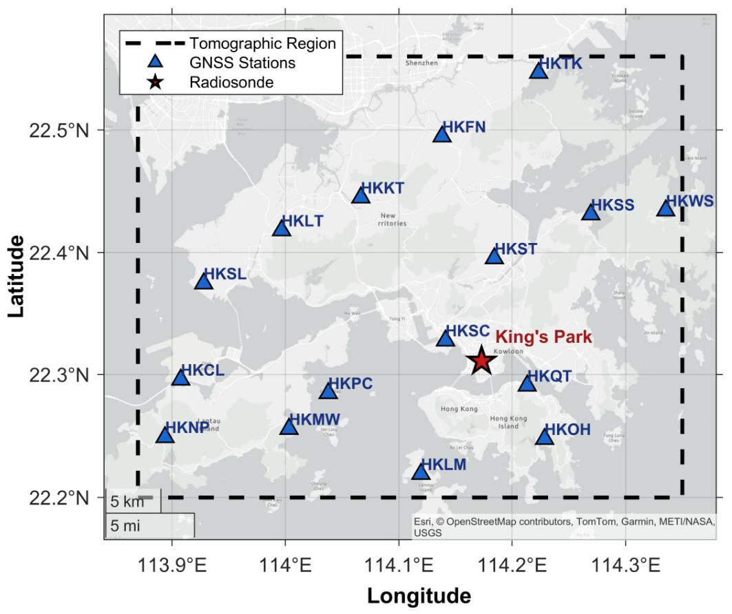
Focusing on the Hong Kong region, which features a relatively dense GNSS network and available radiosonde observations at King’s Park, this study defined the tomographic domain as 22.20–22.56°N and 113.87–114.35°E. A total of 16 GNSS stations were used, and the King’s Park radiosonde station served as the reference site for vertical profile validation. The study area, GNSS station distribution, and the location of the radiosonde station are shown in Figure 1.

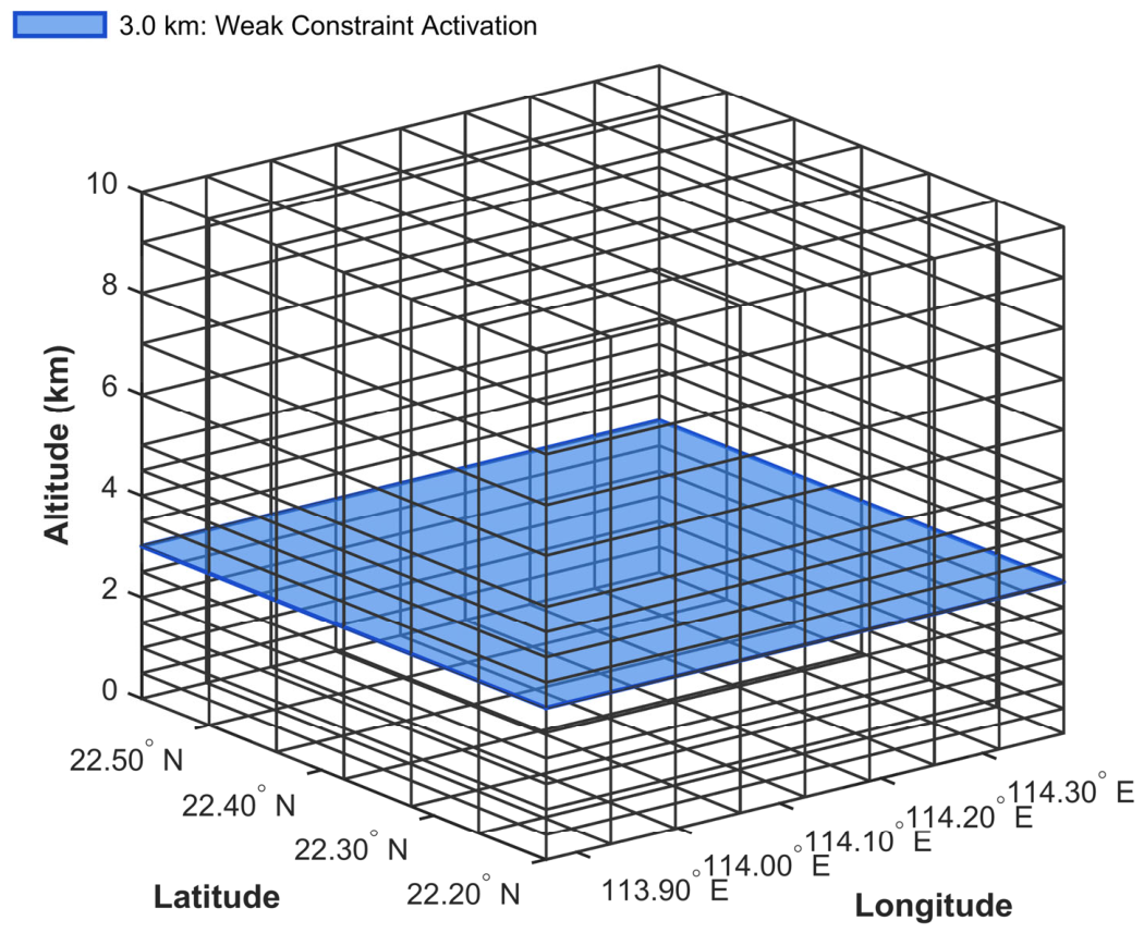
The tomographic space was discretized using a non-uniform three-dimensional voxel grid. The horizontal domain was divided into 6 × 8 grid cells, and the vertical direction was divided into 15 layers. Among them, 10 layers were arranged below 5 km and 5 layers were arranged above 5 km, so that rapid water vapor variation in the lower troposphere could be represented more effectively. The horizontal and vertical grid structures are illustrated in Figure 2.

2.2. Datasets

2.2.1. GNSS Observations

The temporal resolution of the raw GNSS observations was 30 s, and multi-GNSS data from GPS, GLONASS, Galileo, and BDS were processed using the PRIDE PPP-AR software (Wuhan University, Wuhan, China; available online: https://github.com/PrideLab/PRIDE-PPPAR, accessed on 25 May 2026) [25,26]. The zenith wet delay (ZWD) at each epoch was obtained directly from the PPP solution, in which the residual wet tropospheric delay was estimated as an unknown tropospheric parameter during PPP processing. The detailed PPP processing strategy adopted in this study, based on which the ZWD was derived, is summarized in

Table 1. Summary of the main GNSS data processing strategy.

Parameter	Strategies
Satellite systems	GPS, GLONASS, Galileo, BDS
Raw sampling interval	30 s
Positioning mode	Kinematic
Observation cut-off angle	10°
Ionospheric delay	Dual-frequency ionosphere-free combination
Tropospheric mapping function	GMF
Zenith hydrostatic delay	Saastamoinen
Zenith wet delay	Random-walk process

.

2.2.2. FY-4B/GIIRS AVP

The satellite data used in this study were the FY-4B/GIIRS Level-2 atmospheric vertical profile product (AVP). Retrieved from the Geostationary Interferometric Infrared Sounder onboard FY-4B, this product provides atmospheric profile information including temperature, humidity, and geopotential height. Previous studies have shown that the FY-4B/GIIRS AVP has a nadir spatial resolution of about 12 km, a temporal resolution of about 2 h, and 101 pressure levels in the vertical direction, covering the range from about 1000 to 0.005 hPa. The product also includes quality flags [18,22].

2.2.3. Background and Reference Data

Two types of background fields were used in this study. One was the three-day radiosonde-mean background field, constructed from a sliding average of radiosonde profiles during the 72 h preceding each target tomographic epoch. This background was intended to represent the local short-term statistical state without introducing future information. The other was the operational GFS background field, which provided a numerical-model background with stronger spatial continuity. Radiosonde profiles from King’s Park were used as the vertical reference for validation, and ERA5 three-dimensional reanalysis data were used to evaluate the spatial distribution of the tomographic results [27].

3. Methodology

3.1. GNSS Water Vapor Tomography Framework

In this study, the zenith wet delay (ZWD) at each epoch was obtained directly from the PPP solution as described in Section 2.2.1. After ZWD was derived, it was mapped to the signal propagation direction using the satellite elevation angle, azimuth angle, and wet gradient terms, and the SWD was calculated as

$$\mathrm{S}\mathrm{W}\mathrm{D}={\mathrm{M}}_{\mathrm{w}}\left(\mathrm{e}\right)\cdot \mathrm{Z}\mathrm{W}\mathrm{D}+{\mathrm{M}}_{\mathsf{\Delta }}\left(\mathrm{e}\right)\cdot \left({\mathrm{G}}_{\mathrm{N}}^{\mathrm{w}}\cos \mathrm{A}+{\mathrm{G}}_{\mathrm{E}}^{\mathrm{w}}\sin \mathrm{A}\right)$$

(1)

where ${\mathrm{M}}_{\mathrm{w}}\left(\mathrm{e}\right)$ is the wet mapping function, for which GMF was adopted in this study; ${\mathrm{M}}_{\mathsf{\Delta }}\left(\mathrm{e}\right)$ is the gradient mapping function; ${\mathrm{G}}_{\mathrm{N}}^{\mathrm{w}}$ and ${\mathrm{G}}_{\mathrm{E}}^{\mathrm{w}}$ denote the northward and eastward wet delay gradients, respectively; and $\mathrm{e}$ and $\mathrm{A}$ are the satellite elevation angle and azimuth angle. This procedure is consistent with the standard workflow used in previous GNSS water vapor tomography studies [1,4,8,10].

After SWD was obtained, it was converted into SWV using the conversion coefficient $\mathsf{\Pi }$, which is related to the weighted mean temperature ${\mathrm{T}}_{\mathrm{m}}$:

$$\mathrm{S}\mathrm{W}\mathrm{V}=\mathsf{\Pi }\cdot \mathrm{S}\mathrm{W}\mathrm{D}$$

(2)

The SWV values derived in this way were finally used as the tomographic observations for the GNSS-dominant three-dimensional water vapor reconstruction. At each tomographic epoch, the GNSS observation matrix $\mathrm{A}$ was constructed according to the visible satellites and station coordinates. For each valid signal, the tomographic equation was built from the intersection length of the signal within the three-dimensional voxel space. Only valid rays that completely passed through the tomographic domain were retained, namely signals that crossed both the lower and upper boundaries of the region. The tomographic observation equation can therefore be written as

$$\mathrm{A}\mathrm{x}=\mathrm{d}$$

(3)

where $\mathrm{x}$ is the voxel water vapor density vector to be estimated, and $\mathrm{d}$ is the column vector composed of all valid SWV observations at the corresponding epoch. This modeling strategy is consistent with previous regional tomography methods based on SWV [8,28].

3.2. FY-4B/GIIRS AVP Weak-Constraint Construction

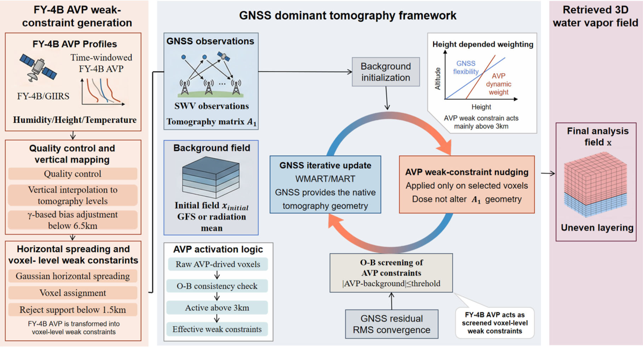
To incorporate the AVP into the tomographic inversion in a stable and controlled manner, the satellite information was not introduced as additional rays or additional observation equations. Instead, it was converted into voxel-level weak constraints, as illustrated in Figure 3. Prior to vertical interpolation, the quality flags provided with the FY-4B/GIIRS Level-2 AVP were applied to exclude retrievals flagged as cloud-contaminated or otherwise unreliable, providing a first-order screening of cloud-affected profiles.

For each target epoch, a matching time window was first defined. In the 00 UTC tomography, the AVP closest to the target time was selected within the 23:00–01:00 window; for the 12 UTC tomography, the nearest profile was selected within the 11:00–13:00 window. This step was intended to maximize temporal consistency with the tomographic epoch rather than to average several satellite scenes. Given the approximately 2 h temporal resolution of the product, selecting the nearest observation within a matching window was consistent with the actual processing strategy adopted here [16,29].

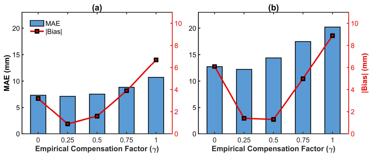
After quality control, the humidity profiles were vertically interpolated from the native pressure levels to the tomographic layers. Because FY-4 moisture-related products can exhibit non-negligible systematic biases and condition-dependent errors, especially in humid environments, a layer-wise compensation strategy was introduced before the AVP was used as a weak constraint [16,18,29]. In Figure 4, the Bias and MAE used to determine γ were computed from differences between AVP-integrated PWV and reference PWV, and are therefore expressed in millimeters. This step was intended to determine the most suitable correction strength rather than to assess water vapor density error in the three-dimensional tomographic field.

Following vertical correction, the satellite pixels were mapped to neighboring voxels with a horizontal Gaussian kernel. The maximum spreading radius was set to 15 km and the Gaussian parameter to 8 km, allowing information from an individual pixel to spread to nearby voxels and thereby reducing the discreteness associated with direct assignment. To match the native spatial resolution of the FY-4B/GIIRS sensor, which is approximately 12 km at nadir [19], the standard deviation of the horizontal Gaussian kernel was empirically set to 8 km, with a maximum spreading radius of 15 km.

Before introducing FY-4B/GIIRS AVP weak constraints, a background-consistency screening step was applied using the background field as the initial analysis field ${\mathrm{x}}_{\mathrm{i}\mathrm{n}\mathrm{i}\mathrm{t}\mathrm{i}\mathrm{a}\mathrm{l}}$. Only those AVP voxel constraints whose difference from the background field satisfied the following threshold were retained:

$$\left|b_{\mathrm{A}\mathrm{V}\mathrm{P}}-x_{\mathrm{i}\mathrm{n}\mathrm{i}\mathrm{t}\mathrm{i}\mathrm{a}\mathrm{l}}\right|\le 1.5 \mathrm{g} {\mathrm{m}}^{-3}$$

(4)

where $b_{\mathrm{A}\mathrm{V}\mathrm{P}}$ denotes the voxel constraint value provided by FY-4B/GIIRS AVP. Through this step, only AVP voxels that were reasonably consistent with the background field were allowed to enter the subsequent weak-constraint update. The 1.5 g/m³ threshold was used here as a practical Observation-minus-Background (O-B) screening criterion to reduce the influence of severe outliers caused by residual cloud contamination or infrared retrieval failures while retaining valid mid-level moisture increments. Its adoption was also consistent with previous validation studies showing that FY-4A/FY-4B GIIRS retrieval performance degrades markedly in the lower troposphere and under cloud-affected conditions [18,30,31,32].

Furthermore, previous operational evaluations and validation studies have shown that FY-4A/FY-4B GIIRS profile retrievals are less reliable in the lower troposphere, where retrieval uncertainty is more strongly affected by surface emissivity, boundary-layer clouds, and the limited vertical discrimination of low-level infrared channels [18,22,30,32,33]. Together with the already strong native GNSS constraints in the lower troposphere, these considerations motivated the activation of AVP weak constraints only above 3.0 km in the present study. This threshold was intended to limit the influence of less reliable near-surface retrievals and to focus the AVP weak constraints on the relatively more stable mid-to-upper troposphere. After these preprocessing steps, the satellite profiles were transformed into a voxel-level weak-constraint field containing the locations of valid constrained voxels, the corresponding constraint values, and the voxel-level weighting factors.

3.3. Model Implementation

The background field was used as the initial analysis field. On this basis, the tomographic solution was obtained within a GNSS-dominant framework enhanced by weak constraints from the AVP. GNSS updates followed a smooth multiplicative iterative strategy based on the multiplicative algebraic reconstruction technique (MART) and its weighted form, weighted MART (WMART). For each valid GNSS ray, the voxel state was updated according to the ratio between observed and simulated SWV. Specifically, the WMART update for voxel k with respect to ray i follows the standard multiplicative form:

$$x_k^{(n+1)}=x_k^{\left(n\right)}\cdot {\left({\displaystyle \frac{y_i}{{\widehat{y}}_i^{\left(n\right)}}}\right)}^{{\lambda }_k\cdot {\displaystyle \frac{a_{ik}}{{‖A_i‖}^2}}}$$

(5)

where ${\widehat{y}}_i^{\left(n\right)}={\sum }_k{a}_{ik}{x}_k^{\left(n\right)}$ is the simulated SWV at iteration $n,y_i$ is the observed SWV, $a_{ik}$ is the intersection length of ray i through voxel k, $\Vert A_i{\Vert }^2={\sum }_k{a}_{ik}^2$ is the squared norm of the i-th row of the observation matrix, and ${\lambda }_k$ is a relaxation parameter.

To limit update amplitude and avoid excessive compression of water vapor in the lower troposphere, a relaxation factor that increased linearly with height was introduced, rising from about 0.1 near the surface to 1.0 near 10 km.

This height-dependent relaxation is implemented by defining ${\lambda }_k$ as:

$${\lambda }_k=\max \left(0.1, \min \left(1.0, 0.1+0.9\cdot {\displaystyle \frac{h_k}{10.0}}\right)\right)$$

(6)

where $h_k$ is the altitude of voxel k in kilometres, and the resulting relaxation factor ${\lambda }_k$ is bounded between 0.1 and 1.0. This strategy preserved relatively conservative updates at low levels while allowing greater flexibility aloft, consistent with previous studies on constraint optimization in water vapor tomography [2,34].

For the AVP component, strong constraints were not imposed on all voxels. Instead, multiplicative nudging was applied only to voxels that had passed the background-consistency screening.

The AVP nudging update for a screened voxel k takes a multiplicative form analogous to MART:

$$x_k^{(n+1)}=x_k^{\left(n\right)}\cdot {\left({\displaystyle \frac{b_k^{\mathrm{A}\mathrm{V}\mathrm{P}}}{x_k^{\left(n\right)}}}\right)}^{w_k^{\mathrm{A}\mathrm{V}\mathrm{P}}}$$

(7)

where $b_k^{\mathrm{A}\mathrm{V}\mathrm{P}}$ is the voxel-level AVP constraint value, the ratio $b_k^{\mathrm{A}\mathrm{V}\mathrm{P}}/x_k^{\left(n\right)}$ is constrained to $[0.9, 1.1]$ to prevent excessive forcing, and the effective AVP weight $w_k^{\mathrm{A}\mathrm{V}\mathrm{P}}$ is defined as:

$$w_k^{\mathrm{A}\mathrm{V}\mathrm{P}}=w_{\mathrm{a}\mathrm{l}\mathrm{t}}\left(h_k\right)\cdot {\alpha }_k$$

(8)

Here ${\alpha }_k$ is the voxel-level weighting factor determined by the horizontal Gaussian spreading, and $w_{\mathrm{a}\mathrm{l}\mathrm{t}}\left(h_k\right)$ is the altitude-dependent dynamic weight:

$$w_{\mathrm{a}\mathrm{l}\mathrm{t}}(h_k)=\left\{\begin{array}{c}0,h_k<3.0 \mathrm{km}\\ 0.05\times {\displaystyle \frac{h_k-3.0}{10.0-3.0}},3.0 \mathrm{km}\le h_k\le 10.0 \mathrm{km}\end{array}\right.$$

(9)

The basic weight increased linearly between 3 and 10 km, reaching a maximum of 0.05. In MART-based tomographic inversions, the relaxation factor must be strictly constrained to maintain mathematical stability [9]. This conservative maximum weight was adopted to preserve the GNSS-dominant character of the framework and to avoid excessive forcing from the AVP component. It ensures that the AVP provides only soft nudging rather than overwhelming the high-precision native GNSS ray geometry [3,9]. The effective weight assigned to each constrained voxel was determined jointly by the altitude-dependent dynamic weight and the voxel-level weighting factor. In practice, the AVP therefore acted mainly as a weak constraint for the middle and upper troposphere rather than as a source of strong direct forcing at lower levels.

A maximum of 100 iterations was allowed for each epoch. The convergence criterion was defined by the change in GNSS observation residuals between successive iterations. Once the number of iterations exceeded 15 and the residual change between two successive iterations fell below a prescribed tolerance of ${10}^{-5}$, the current epoch was considered to have reached stable convergence. The final outputs included the three-dimensional voxel water vapor density field, the GNSS observation matrix, the residual convergence sequence, and the background initial field.

3.4. Evaluation Metrics

The tomographic results were evaluated from four aspects, namely absolute accuracy, layer-wise accuracy, temporal stability, and spatial improvement. For radiosonde profile validation, Bias, mean absolute error (MAE), root mean square error (RMSE), and relative RMSE were used to describe the error level of different schemes. Let ${\mathrm{x}}_{\mathrm{i}}^{\mathrm{t}\mathrm{o}\mathrm{m}\mathrm{o}}$ and ${\mathrm{x}}_{\mathrm{i}}^{\mathrm{r}\mathrm{s}}$ denote the water vapor density values from tomography and radiosonde observations, respectively, and let $\mathrm{N}$ be the total number of matched sample points. The statistical metrics were defined as

$$\mathrm{B}\mathrm{i}\mathrm{a}\mathrm{s}={\displaystyle \frac{1}{\mathrm{N}}}{\displaystyle {\sum }_{\mathrm{i}=1}^{\mathrm{N}}}\left({\mathrm{x}}_{\mathrm{i}}^{\mathrm{t}\mathrm{o}\mathrm{m}\mathrm{o}}-{\mathrm{x}}_{\mathrm{i}}^{\mathrm{r}\mathrm{s}}\right)$$

(10)

$$\mathrm{M}\mathrm{A}\mathrm{E}={\displaystyle \frac{1}{\mathrm{N}}}{\displaystyle {\sum }_{\mathrm{i}=1}^{\mathrm{N}}}\left|{\mathrm{x}}_{\mathrm{i}}^{\mathrm{t}\mathrm{o}\mathrm{m}\mathrm{o}}-{\mathrm{x}}_{\mathrm{i}}^{\mathrm{r}\mathrm{s}}\right|$$

(11)

$$\mathrm{R}\mathrm{M}\mathrm{S}\mathrm{E}=\sqrt{{\displaystyle \frac{1}{\mathrm{N}}}{\displaystyle {\sum }_{\mathrm{i}=1}^{\mathrm{N}}}{\left({\mathrm{x}}_{\mathrm{i}}^{\mathrm{t}\mathrm{o}\mathrm{m}\mathrm{o}}-{\mathrm{x}}_{\mathrm{i}}^{\mathrm{r}\mathrm{s}}\right)}^2}$$

(12)

$$\mathrm{r}\mathrm{e}\mathrm{l}\mathrm{a}\mathrm{t}\mathrm{i}\mathrm{v}\mathrm{e}\hspace{0.25em}\mathrm{R}\mathrm{M}\mathrm{S}\mathrm{E}={\displaystyle \frac{\mathrm{R}\mathrm{M}\mathrm{S}\mathrm{E}}{\overline{{\mathrm{x}}^{\mathrm{r}\mathrm{s}}}}}\times 100\mathrm{\%}$$

(13)

where $\overline{{\mathrm{x}}^{\mathrm{r}\mathrm{s}}}$ is the mean radiosonde water vapor density of the corresponding matched samples.

RMSE was calculated in two ways:

The first is the global point-wise RMSE, denoted ${\mathrm{R}\mathrm{M}\mathrm{S}\mathrm{E}}_{\mathrm{g}\mathrm{l}\mathrm{o}\mathrm{b}\mathrm{a}\mathrm{l}}$ which pools all matched sample points across all vertical layers into a single calculation:

$${\mathrm{R}\mathrm{M}\mathrm{S}\mathrm{E}}_{\mathrm{g}\mathrm{l}\mathrm{o}\mathrm{b}\mathrm{a}\mathrm{l}}=\sqrt{{\displaystyle \frac{1}{N}}{\sum }_{i=1}^N{\left(x_i^{\mathrm{t}\mathrm{o}\mathrm{m}\mathrm{o}}-x_i^{\mathrm{r}\mathrm{s}}\right)}^2}$$

(14)

where $N$ is the total number of matched points across all layers and all epochs. This metric reflects the overall absolute error of the tomographic field as a whole.

The second is the layer-averaged RMSE, denoted ${\mathrm{R}\mathrm{M}\mathrm{S}\mathrm{E}}_{\mathrm{l}\mathrm{a}\mathrm{y}\mathrm{e}\mathrm{r}-\mathrm{a}\mathrm{v}\mathrm{g}}$, which is obtained by first computing RMSE independently within each vertical layer and then averaging the per-layer values across all layers:

$${\mathrm{R}\mathrm{M}\mathrm{S}\mathrm{E}}_{\mathrm{l}\mathrm{a}\mathrm{y}\mathrm{e}\mathrm{r}-\mathrm{a}\mathrm{v}\mathrm{g}}={\displaystyle \frac{1}{L}}{\sum }_{k=1}^L\sqrt{{\displaystyle \frac{1}{n_k}}{\sum }_{j=1}^{n_k}{\left(x_{k,j}^{\mathrm{t}\mathrm{o}\mathrm{m}\mathrm{o}}-x_{k,j}^{\mathrm{r}\mathrm{s}}\right)}^2}$$

(15)

where $L$ is the number of vertical layers and $n_k$ is the number of matched samples in the $k$-th layer. Because each layer contributes equally to the average regardless of its sample size, this metric places greater emphasis on the vertical structure of the error than ${\mathrm{R}\mathrm{M}\mathrm{S}\mathrm{E}}_{\mathrm{g}\mathrm{l}\mathrm{o}\mathrm{b}\mathrm{a}\mathrm{l}}$ does. These two statistics are not numerically equivalent because they follow different aggregation paths, but they represent overall absolute error and average vertical-structure error, respectively.

4. Experiments and Results

4.1. Experimental Design

To systematically evaluate the effects of FY-4B/GIIRS AVP weak constraints and background-field type on the tomographic results, four comparative experiments were designed:

Tomo-I: Three-day radiosonde-mean background field, without AVP.

Tomo-II: Three-day radiosonde-mean background field, with AVP weak constraints.

Tomo-III: GFS background field, without AVP.

Tomo-IV: GFS background field, with AVP weak constraints.

This design forms a two-factor experimental framework, namely background-field type and whether AVP weak constraints are introduced. It allows the contribution of the background field itself and the additional contribution of FY-4B/GIIRS AVP to be evaluated separately.

4.2. Bias Correction of FY-4B/GIIRS AVP and Determination of the Compensation Factor

Before introducing FY-4B/GIIRS AVP into the tomographic inversion, its systematic error during the study period was first evaluated, and the compensation factor used in this study was then determined. Figure 4 shows the variations in Bias and MAE under different values of $\mathsf{\gamma }$. Here, the reference PWV was obtained by vertically integrating the specific humidity from the King’s Park radiosonde profiles over the tomographic altitude range of 0–10 km. The Bias and MAE reported here were calculated from the differences between PWV integrated from FY-4B/GIIRS AVP and the reference PWV, and are therefore expressed in millimeters.

Figure 4 shows that the uncorrected AVP ($\mathsf{\gamma }=0$) exhibited clear systematic dry biases of −3.34 mm and −6.20 mm at 12 UTC and 00 UTC, respectively. As $\mathsf{\gamma }$ increased, the absolute value of Bias gradually decreased, whereas MAE first decreased and then increased. When $\mathsf{\gamma }=0.25$, the Bias at 12 UTC and 00 UTC improved to −0.89 mm and −1.42 mm, respectively, while the MAE decreased to 7.10 mm and 12.21 mm, giving the best balance among the tested values.

Accordingly, $\mathsf{\gamma } = 0.25$ was selected as the final compensation factor for the AVP, and it was applied to the layer-wise correction below 10 km.

4.3. Effect of FY-4B/GIIRS AVP Weak Constraints on Effective Support Coverage

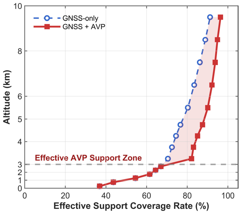
As shown in Figure 5, the support enhancement introduced by the AVP shows a clear height dependence. Below 3 km, the two curves almost overlap, indicating that the lower levels are still mainly controlled by the native GNSS constraints. Between 3 and 5 km, the increase in coverage becomes most evident and reaches a maximum at 3.25 km, where the coverage rises from 70.5% to 82.1%, corresponding to an increase of 11.6 percentage points. At higher levels, although the GNSS-only coverage is already relatively high, the AVP still provides a positive additional contribution. For example, at 9.5 km, the coverage further increases from 91.2% to 96.4%.

These results show that the AVP provides additional effective support mainly in the middle and upper troposphere.

4.4. AVP-Induced Analysis Increments and Layer-Wise Error Improvement

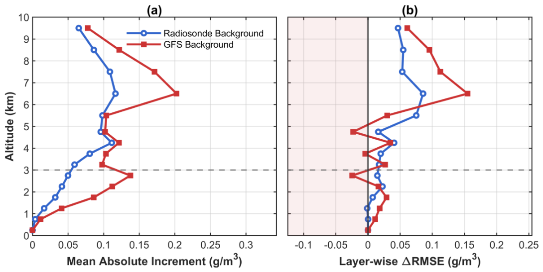
To clarify how the weak constraints affected the vertical structure of the analysis field, layer-wise mean absolute increments between analyses with and without the AVP were compared with layer-wise ΔRMSE. The former identifies the altitude levels at which the satellite profiles produced the main adjustments, while the latter shows whether those adjustments were accompanied by error reduction.

Figure 6a shows that the influence of the AVP was concentrated mainly above 3 km, with the clearest effect appearing in the middle and upper troposphere. Under the GFS background, the analysis increment reached a maximum of 0.202 $\mathrm{g}/{\mathrm{m}}^3$ at 6.50 km, while the corresponding $\mathsf{\Delta }\mathrm{R}\mathrm{M}\mathrm{S}\mathrm{E}$ at the same level reached +0.155 $\mathrm{g}/{\mathrm{m}}^3$. Under the radiosonde background, the improvement at this level was about +0.086 $\mathrm{g}/{\mathrm{m}}^3$. These results show that the AVP-induced correction and the associated error reduction were more evident under the GFS background.

The peak in effective support coverage occurred at 3.25 km, whereas the peak in analysis increment appeared at 6.50 km. This indicates that the altitude of maximum added support was not identical to the altitude of maximum analysis response. The physical mechanisms underlying this height-dependent response are discussed further in Section 5.2.

Small but non-zero increments were also found in the lower troposphere. Although the weak constraints were activated mainly above 3 km, a limited response was still observed below this level. The principal benefit, however, remained concentrated in the middle and upper troposphere.

4.5. Vertical Accuracy Comparison Among the Four Tomographic Schemes

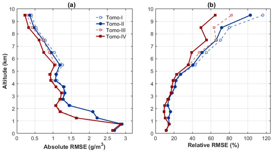
The absolute error characteristics of the four schemes in terms of overall vertical structure were further compared using the layer-wise RMSE and relative RMSE profiles shown in Figure 7.

Based on the radiosonde-referenced vertical statistics, the background-field type appears to be the primary factor controlling the absolute accuracy of the tomographic results, while the AVP provides additional improvement on this basis. Over the full altitude range (0–10 km), the absolute RMSE values of Tomo-I, Tomo-II, Tomo-III, and Tomo-IV are 1.43, 1.40, 1.22, and 1.18 $\mathrm{g}/{\mathrm{m}}^3$, respectively, and the corresponding relative RMSE values are 36.0%, 33.6%, 29.5%, and 26.0%. Among the four schemes, Tomo-IV achieves the best performance in both indices.

A more detailed layer-wise comparison further shows that the improvement is limited in the lower troposphere, whereas it is more evident in the middle and upper troposphere. In the middle and upper levels, the absolute RMSE values of the four schemes are 0.98, 0.94, 0.84, and 0.79 $\mathrm{g}/{\mathrm{m}}^3$, respectively, while the corresponding relative RMSE values are 50.5%, 46.6%, 41.4%, and 35.6%. Compared with Tomo-I, Tomo-IV reduces the relative RMSE in the middle and upper troposphere by 14.9 percentage points. Even when compared with the GFS-only scheme Tomo-III, Tomo-IV still provides an additional reduction of 5.8 percentage points.

These results show that the GFS background field provides the main improvement in the radiosonde-referenced vertical evaluation, while the AVP weak constraints provide an additional gain, especially in the middle and upper troposphere. The larger gain observed under the GFS background is discussed further in Section 5.3.

4.6. Point-to-Point Consistency with Radiosonde Observations

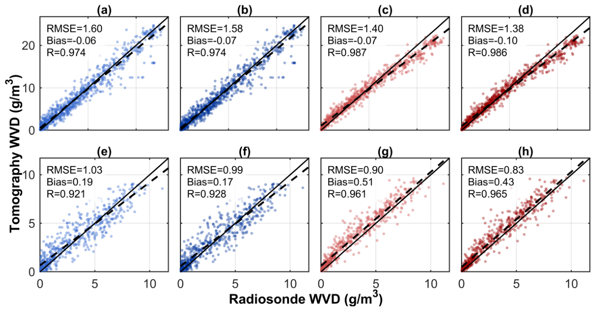
To evaluate the overall agreement between the four schemes and the radiosonde profiles, all matched sample pairs across all epochs during the study period (August 2024, 62 epochs in total) and all matched vertical layers within the 0–10 km range were pooled to generate point-to-point density scatterplots (N = 930 per scheme). A separate set of scatterplots was generated using only the layers above 3 km (N = 558 per scheme) to highlight the performance in the middle and upper troposphere, as shown in Figure 8.

Over the full altitude range, the global point-wise RMSE values of Tomo-I, Tomo-II, Tomo-III, and Tomo-IV are 1.60, 1.58, 1.40, and 1.38 $\mathrm{g}/{\mathrm{m}}^3$, respectively, indicating that the schemes using the GFS background are generally closer to the radiosonde observations. When only the middle and upper troposphere is considered, the RMSE values decrease to 1.03, 0.99, 0.90, and 0.83 $\mathrm{g}/{\mathrm{m}}^3$, respectively. Among them, Tomo-IV gives the lowest RMSE, while the correlation coefficient increases to 0.965.

These results show better point-to-point agreement with the radiosonde observations after introducing FY-4B/GIIRS AVP weak constraints, particularly in the middle and upper troposphere.

4.7. Temporal Stability of the Additional Benefit from FY-4B/GIIRS AVP

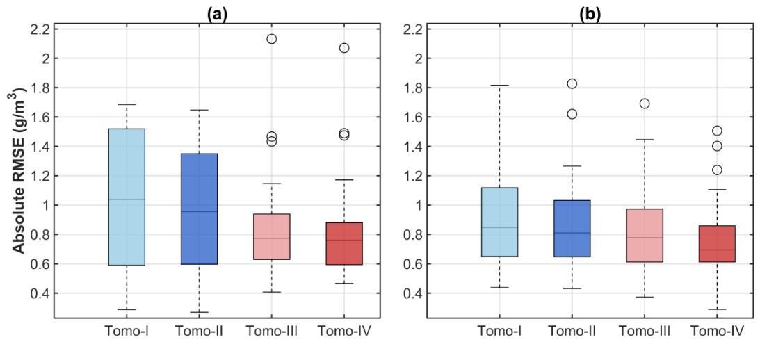
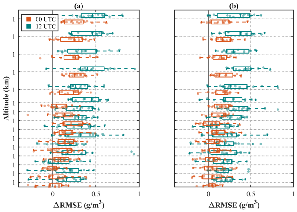
To evaluate the temporal stability of the AVP weak constraints, the epoch-by-epoch RMSE distributions at 00 UTC and 12 UTC were analyzed (Figure 9), and the variation in the AVP-induced error improvement at the epoch scale was further examined using the $\mathsf{\Delta }\mathrm{RMSE}$ distributions (Figure 10).

The boxplots show that the absolute RMSE distributions under the GFS background are generally lower than those under the radiosonde-mean background. Under the same background-field condition, the box positions usually shift slightly downward after FY-4B/GIIRS AVP is introduced, indicating that FY-4B/GIIRS AVP provides relatively stable additional benefits at the epoch scale. In particular, at 12 UTC, Tomo-IV reaches a mean error of 0.755 $\mathrm{g}/{\mathrm{m}}^3$, together with the smallest standard deviation of 0.281, which indicates a favorable combination of accuracy and stability.

The distribution of $\mathsf{\Delta }\mathrm{R}\mathrm{M}\mathrm{S}\mathrm{E}$ further shows that positive values dominate, which indicates that the improvement brought by the AVP is not controlled by a few extreme cases but is present in a considerable number of epochs. In addition, the $\mathsf{\Delta }\mathrm{RMSE}$ distribution at 12 UTC is generally better than that at 00 UTC, suggesting that the AVP weak constraints tended to be more effective in the 12 UTC epochs examined here. Although the boxplot distributions and the dominance of positive $\mathsf{\Delta }\mathrm{R}\mathrm{M}\mathrm{S}\mathrm{E}$ values suggest a consistent improvement across most epochs, formal significance testing was not performed in this study.

4.8. Typical Radiosonde Profile Cases Under Clear-Sky and Rainfall Conditions

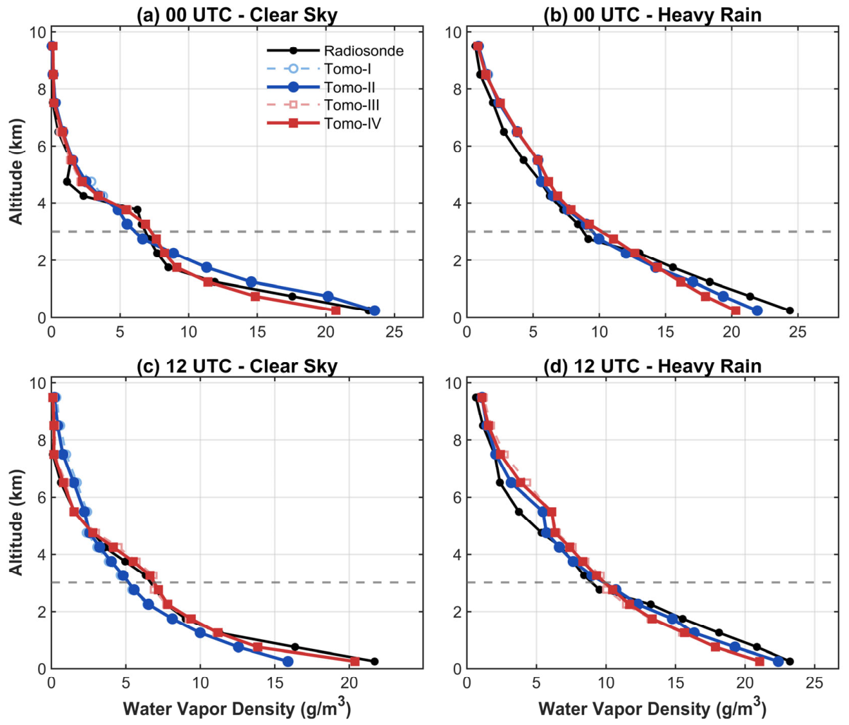
To further illustrate the role of the AVP weak constraints under different weather conditions, two clear-sky cases and two heavy-rainfall cases were selected, and the profiles from the four schemes were compared with the radiosonde observations in Figure 11. The case selection was based on the daily weather records of the Hong Kong Observatory and the completeness of the radiosonde data. The two heavy-rainfall cases (18 and 19 August 2024) were chosen from a multi-day persistent rainstorm episode and represent the most convectively active conditions within the study period, while the two clear-sky cases were selected from days recorded as fine weather with no rainfall. All four selected epochs have complete King’s Park radiosonde profiles available for validation.

The case analysis shows that, in both the clear-sky and the heavy-rainfall cases, the profiles from the AVP-constrained schemes (Tomo-II and Tomo-IV) were generally closer to the radiosonde observations than their no-AVP counterparts (Tomo-I and Tomo-III), particularly in the middle and upper troposphere above 3 km. The adjustments introduced by the AVP weak constraints consistently acted to reduce the deviation between the analysis profiles and the radiosonde reference. In the heavy-rainfall cases, where the moisture field was more convectively disturbed, the AVP weak constraints removed up to 19.0–23.5% of the background error in the affected mid- and upper-tropospheric layers, indicating that the additional benefit of the AVP remained effective even under intense rainfall conditions. These case comparisons show that the improvement introduced by the AVP weak constraints was not restricted to a particular weather type, but was present under both clear-sky and heavy-rainfall conditions.

To further assess the performance of the AVP weak constraints under heavy-rainfall conditions, all 12 epochs during the persistent rainstorm episode of 15–20 August 2024 were examined, and the layer-wise RMSE above 3 km was computed for each epoch with and without the AVP. After the AVP weak constraints were introduced, the RMSE above 3 km did not increase in any of the 12 epochs. About two-thirds of the epochs showed a positive improvement, while the remaining epochs showed essentially unchanged results, mainly because the strict quality-flag and O-B screening removed cloud-contaminated AVP retrievals during the most intense rainfall periods. Under the GFS background, the mean $\mathsf{\Delta }\mathrm{R}\mathrm{M}\mathrm{S}\mathrm{E}$ during this episode was +0.038 g/m³. Although this analysis covers only a single multi-day rainstorm episode and the sample is therefore limited, the results suggest that the AVP weak constraints did not degrade the tomographic accuracy under heavy-rainfall conditions and still provided a positive contribution in most cases.

4.9. Spatial Evaluation of the Four Tomographic Schemes

In addition to vertical profile validation, ERA5 three-dimensional reanalysis data were used to evaluate the spatial distribution of the tomographic results. Radiosonde observations provide only single-column validation, whereas ERA5 offers a continuous three-dimensional reference field. It can therefore be used to describe the overall spatial error distribution of different tomographic schemes within the study region.

ERA5-based evaluation thus serves as a spatial complement to the single-station radiosonde validation, allowing the overall spatial error distribution of the tomographic field to be described beyond the King’s Park column.

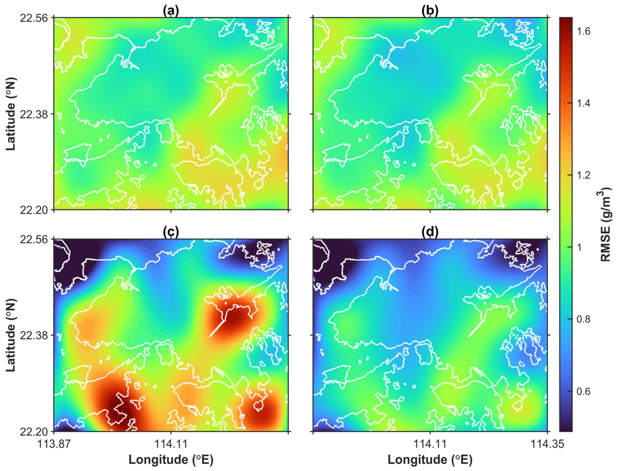
Figure 12 shows that spatial performance did not improve monotonically when the radiosonde-mean background was replaced by GFS. Although Tomo-IV achieved the lowest spatial RMSE, Tomo-III was slightly worse than Tomo-I in terms of ERA5-referenced spatial mean RMSE.

From the regional mean statistics, the spatial mean RMSE values of Tomo-I and Tomo-II under the radiosonde-mean background are 0.937 $\hspace{0.17em}\mathrm{g}/{\mathrm{m}}^3$ and 0.912 $\hspace{0.17em}\mathrm{g}/{\mathrm{m}}^3$, respectively. Under the GFS background, the corresponding spatial mean RMSE values of Tomo-III and Tomo-IV are 0.996 $\hspace{0.17em}\mathrm{g}/{\mathrm{m}}^3$ and 0.827 $\hspace{0.17em}\mathrm{g}/{\mathrm{m}}^3$, respectively. These results indicate that FY-4B/GIIRS AVP weak constraints provide positive gains under both types of background fields, while the absolute improvement is more pronounced under the GFS background.

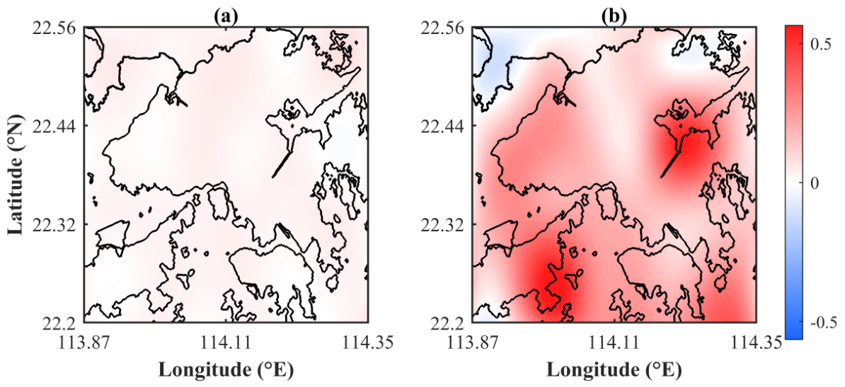
To show the spatial benefit brought by the AVP weak constraints more directly, the spatial distribution of $\mathsf{\Delta }\mathrm{R}\mathrm{M}\mathrm{S}\mathrm{E}$ before and after the introduction of AVP was further calculated, where positive values indicate a reduction in error after AVP is introduced.

As shown in Figure 13, the spatial benefit of the AVP weak constraints is not limited to only a few local grids. Positive gains are found over most parts of the study region. Under the radiosonde-mean background, the upgrade from Tomo-I to Tomo-II leads to a spatial mean RMSE improvement of 0.024 $\hspace{0.17em}\mathrm{g}/{\mathrm{m}}^3$, corresponding to a relative improvement of 2.60%. At the same time, the proportion of grids showing positive improvement reaches 97.9%. Under the GFS background, the upgrade from Tomo-III to Tomo-IV increases the spatial mean RMSE improvement to 0.169 $\hspace{0.17em}\mathrm{g}/{\mathrm{m}}^3$, corresponding to a relative improvement of 16.96%, while the proportion of grids with positive improvement is 93.8%.

These results show that the AVP weak constraints provide positive spatial gains under both background fields, with larger improvement under the GFS background.

5. Discussion

5.1. Methodological Role of FY-4B/GIIRS AVP

The methodological role of the AVP in this study was clearly defined. It did not enter the tomography as an additional ray, nor was it inserted into the GNSS observation matrix. Instead, the satellite profiles provided screened weak constraints for voxels in the middle and upper troposphere. The resulting gain was therefore expressed not as a modification of native GNSS geometry, but as stronger effective support within the analysis space and improved vertical structure aloft.

This distinguishes the present work from earlier studies that combined FY-4A data with GNSS tomography, where the reported improvement was commonly interpreted in terms of observation-system expansion, increased numbers of non-empty voxels, and better geometric coverage [23,24]. The present strategy followed a different logic. Its aim was not to expand the geometry, but to improve analysis stability and the quality of the reconstructed vertical structure. In that sense, it remained conceptually close to earlier studies on constraint optimization and background-field enhancement in regional GNSS tomography [2,23,35,36,37,38,39].

5.2. Dominance of the Improvement in the Mid- and Upper Troposphere

The gains associated with the AVP were concentrated mainly above 3 km and were most evident between 5 and 8 km, a pattern consistent with both the algorithm design and the characteristics of the data.

Part of the explanation lies in the design of the weak constraints themselves. In this study, they were activated only above 3.0 km, and their dynamic weight increased with height. The middle and upper troposphere therefore became the natural region of influence. Native GNSS constraints also tend to be stronger in the lower troposphere, whereas the layers aloft depend more heavily on the background field and smoothing constraints, making them more responsive to external information [9,34].

The nature of the satellite profiles offers a second explanation. The AVP contains vertically resolved structural information rather than only column-integrated moisture, making it more suitable for supplementing middle- and upper-level structure than for replacing the dominant role of GNSS near the surface. Previous studies of FY-4A and FY-4B water vapor products have likewise shown that products carrying vertical profile information tend to be more valuable aloft, while the near-surface layer is more strongly influenced by retrieval uncertainty and surface conditions [14,18,19,22,30,32,40].

The peak of effective support coverage appeared at 3.25 km, while the peak of the analysis increment appeared at 6.50 km. This difference indicates that the altitude of maximum added support was not identical to the altitude of maximum reconstruction response. At 6.50 km, the lower background water vapor density makes a given correction more pronounced in relative terms. More importantly, the larger altitude-dependent weak-constraint weight and the relatively higher reliability of FY-4B/GIIRS retrievals in the mid-troposphere [18,22,30,32] jointly make the reconstruction more responsive to AVP information at this level.

5.3. Dependence on Background Fields

The four experimental schemes made it possible to separate the effect of the background field from the additional contribution of the satellite profiles. The comparison showed that the background field itself remained the primary factor controlling overall accuracy, while the AVP provided further correction on top of that baseline.

The radiosonde-referenced vertical statistics and the ERA5-referenced spatial evaluation showed a partially divergent pattern. For a region such as Hong Kong, where moisture varies rapidly and land–sea contrast is strong, a background field with stronger spatial continuity is more likely to provide a reasonable initial state. Although the GFS background alone (Tomo-III) clearly outperformed the radiosonde-mean background (Tomo-I) in the vertical point-to-point comparisons at King’s Park, its spatial mean RMSE against ERA5 (0.996 $\mathrm{g}/{\mathrm{m}}^3$) was higher than that of Tomo-I (0.937 $\mathrm{g}/{\mathrm{m}}^3$). This spatial mismatch is physically reasonable given that GFS contains richer mesoscale spatial detail than the smoothed radiosonde-mean background, leading to larger differences when compared against ERA5 [27]. However, the introduction of AVP weak constraints (Tomo-IV) markedly reduced this spatial error to 0.827 $\mathrm{g}/{\mathrm{m}}^3$. This suggests that the AVP weak constraints helped reduce part of the spatial structural mismatch associated with the GFS background and improved the ERA5-referenced regional reconstruction in the present experimental setting. Earlier studies have reached similar conclusions, emphasizing that the temporal and spatial continuity of the background field, together with its vertical structural quality, can significantly affect regional tomography [35,41].

A stronger background did not diminish the value of the satellite profiles. Under the GFS background, the AVP still produced clear additional gains in the middle and upper troposphere, with even larger improvements at some levels and in some regions. A plausible explanation is that the higher-quality background made the background-consistency screening more selective, allowing more reliable and more compatible constrained voxels to remain. Fewer constraints, when better placed, could therefore yield more efficient correction. A further mechanism contributing to this difference lies in the O-B screening step itself. A statistical analysis of the O-B distributions across all available epochs in August 2024 shows that the mean O-B value under the GFS background is 0.908 g/m³, compared with 1.116 g/m³ under the radiosonde-mean background, a difference of 0.209 g/m³. This indicates that the GFS background is systematically more consistent with the FY-4B/GIIRS AVP, which can be attributed to the stronger spatial continuity and dynamical structure of GFS—including its horizontal wind, temperature, and moisture fields—that better captures the mesoscale moisture gradients driven by the land–sea contrast characteristic of the Hong Kong region [27]. As a result, the O-B screening admits a higher proportion of valid AVP voxels under the GFS background (80.3% on average) than under the radiosonde-mean background (73.7%), and the epoch-to-epoch variability of the admission rate is also smaller (standard deviation of 12.8% versus 20.5%). This background-dependent screening efficiency provides an additional explanation for the larger AVP-induced improvement observed under the GFS background, beyond the difference in initial field quality alone.

The results thus suggest not that a stronger background weakens the contribution of the AVP, but that the background field defines the baseline quality of the tomographic analysis, while the satellite profiles provide a targeted supplement aloft under the present experimental setting.

5.4. Time Dependence and Weather Dependence

Both the temporal stability analysis and the typical case analysis showed that the weak constraints tended to produce more evident gains at 12 UTC than at 00 UTC. These features suggest that the effect of the AVP weak constraints was not temporally fixed, but depended to some extent on the moisture structure of the selected cases.

A possible explanation is that, in the selected summer cases, the vertical structure of moisture was more variable at 12 UTC, making inter-scheme differences easier to detect. This interpretation is consistent with previous studies in the Hong Kong region [6,22,42], but it should still be regarded as an inference rather than a direct demonstration of this study.

The case studies also showed that the improvement introduced by the AVP weak constraints was present under markedly different weather conditions. Both the clear-sky and the heavy-rainfall cases showed reduced deviation from the radiosonde profiles in the middle and upper troposphere after the AVP was introduced. This indicates that the benefit of the weak constraints was not confined to a specific weather regime, although the magnitude of the adjustment varied from case to case.

5.5. Limitations

Although the results generally support the positive contribution of the weak constraints, several limitations remain. The experiment covered only August 2024, and the study area was limited to Hong Kong. In addition, vertical validation relied primarily on the King’s Park radiosonde station, while the spatial evaluation used ERA5 as a reanalysis reference rather than the true atmospheric state. Several key parameters in the present framework, including the compensation factor, the background-consistency screening threshold, the 3.0 km activation threshold, the weak-constraint weight, and the Gaussian spreading parameters, also retain an empirical character. Cloud contamination was controlled through the official AVP quality flags and the subsequent O-B consistency screening, but an independent quantitative assessment of cloud-dependent retrieval errors was not performed in this study.

The 3.0 km activation threshold and the Gaussian kernel parameters were determined based on the documented retrieval characteristics of FY-4B/GIIRS [14,16,19] and the native GNSS coverage transition discussed in Section 3.2. The O-B screening threshold of 1.5 g/m³ was selected based on a joint sensitivity analysis of the AVP voxel retention rate and the resulting tomographic RMSE under varying threshold values. The results are summarized in

Table 2. Sensitivity of the O-B screening threshold to the retention rate of valid AVP constraint voxels and tomographic RMSE, evaluated under two background fields.

O-B Threshold (g/m3)	GFS Retention (%)	RS-Mean Retention (%)	Tomo-II ΔRMSE (g/m3)	Tomo-IV ΔRMSE (g/m3)
0.5	45.5	38.0	+0.010	+0.018
1.0	66.2	60.4	+0.009	+0.012
1.5 (adopted)	80.3	73.7	0 (ref)	0 (ref)
2.0	88.9	81.8	+0.003	+0.004
3.0	96.1	93.6	+0.003	+0.010

. At thresholds of 0.5 and 1.0 g/m³, the retention rates drop to 45.5% and 66.2% under the GFS background respectively, and the tomographic RMSE increases by up to 0.018 g/m³ relative to the 1.5 g/m³ baseline, indicating that overly strict screening discards valid mid-level moisture increments. At thresholds of 2.0 and 3.0 g/m³, the retention rates exceed 88%, but the tomographic RMSE also increases slightly, suggesting that the additional voxels admitted at these thresholds introduce noise into the weak-constraint update. The threshold of 1.5 g/m³ minimizes the tomographic RMSE under both Tomo-II and Tomo-IV and was therefore adopted as the practical optimum.

Furthermore, the spread in the epoch-by-epoch ΔRMSE distributions indicates that the benefit of the AVP weak constraints is not uniform across all cases, and its statistical significance warrants further evaluation over longer observational periods. The present results should therefore be interpreted as a demonstration of the framework’s potential under summer monsoon conditions rather than as a comprehensive assessment of its performance across all seasons and weather regimes.

Finally, a direct quantitative comparison with other published GNSS tomography models was not performed in this study, as differences in study region, network density, data sources, and background-field type make such comparisons difficult to interpret. Nevertheless, the accuracy levels achieved by the proposed framework are broadly consistent with those reported in representative regional GNSS tomography studies. Full-column radiosonde-referenced RMSE values in the range of approximately 1.1–1.8 g/m³ have been reported in previous tomography studies over Hong Kong and nearby regions under various background-field configurations [2,8,10,23,24], and the present Tomo-IV result of 1.18 g/m³ is within this range. It should be noted that the Tomo-I and Tomo-III schemes in this study themselves correspond to traditional GNSS-only tomography under two different background fields, so the comparison among the four schemes already provides a direct assessment against the conventional approach. On this basis, the main advantage of the proposed framework lies in its targeted improvement in the middle and upper troposphere, achieved without modifying the native GNSS observation geometry.

6. Conclusions

This study developed a FY-4B/GIIRS AVP weak-constraint-enhanced GNSS three-dimensional water vapor tomography framework. The AVP information was first preprocessed and evaluated, and was then incorporated into the tomographic reconstruction as weak constraints. On this basis, a comparative framework under two background fields was established to assess the contribution of FY-4B/GIIRS AVP to regional GNSS water vapor tomography.

The results showed that the uncorrected AVP exhibited a clear systematic dry bias, and a compensation factor of $\mathsf{\gamma }=0.25$ was selected to achieve the best balance between Bias and MAE. After AVP weak constraints were introduced, analysis increments and error reduction were concentrated mainly above 3 km and were more evident under the GFS background. Among the four schemes, Tomo-IV achieved the best overall performance, with the largest improvement (35.6% relative RMSE) concentrated in the middle and upper troposphere. In the spatial evaluation, the introduction of AVP under the GFS background produced a regional mean RMSE improvement of 16.96%.

Overall, the results demonstrate that FY-4B/GIIRS AVP can effectively enhance GNSS water vapor tomography as a weak constraint. Its main contribution lies in providing additional effective support and improving the reconstructed vertical moisture structure, especially in the middle and upper troposphere, without altering the native GNSS observation geometry. Although the present results are encouraging, further validation under different seasons, regions, and weather conditions is still needed to assess the broader applicability of this strategy.

More broadly, the weak-constraint strategy proposed here is relatively simple to implement and potentially compatible with near-real-time GNSS processing pipelines, suggesting a viable pathway toward improved near-real-time three-dimensional water vapor monitoring in support of severe-weather monitoring and forecasting applications in regions with dense GNSS coverage. Future work will prioritize multi-season validation, extension to other regions with FY-4B coverage, and systematic evaluation of the key empirical parameters under varying atmospheric and seasonal conditions.

References

1. Bevis, M.; Businger, S.; Herring, T.A.; Rocken, C.; Anthes, R.A.; Ware, R.H. GPS meteorology: Remote sensing of atmospheric water vapor using the global positioning system. J. Geophys. Res. Atmos. 1992, 97, 15787–15801. [Google Scholar] [CrossRef]
2. Bevis, M.; Businger, S.; Chiswell, S.; Herring, T.A.; Anthes, R.A.; Rocken, C.; Ware, R.H. GPS meteorology: Mapping zenith wet delays onto precipitable water. J. Appl. Meteorol. Climatol. 1994, 33, 379–386. [Google Scholar] [CrossRef]
3. Bender, M.; Raabe, A. Preconditions to ground based GPS water vapour tomography. Ann. Geophys. 2007, 25, 1727–1734. [Google Scholar] [CrossRef]
4. Perler, D.; Geiger, A.; Hurter, F. 4D GPS water vapor tomography: New parameterized approaches. J. Geod. 2011, 85, 539–550. [Google Scholar] [CrossRef]
5. Rocken, C.; Van Hove, T.; Ware, R. Near real-time GPS sensing of atmospheric water vapor. Geophys. Res. Lett. 1997, 24, 3221–3224. [Google Scholar] [CrossRef]
6. Qiu, H.; Yin, W.; Zhou, C.; Tian, Y.; Kong, J.; Chen, H.; Liu, P.; Yao, Y. Spatiotemporal analysis of GNSS-derived water vapor variations and moisture convergence mechanism during extreme rainfall events: A Hong Kong case study. IEEE J. Sel. Top. Appl. Earth Obs. Remote Sens. 2025, 18, 23061–23071. [Google Scholar] [CrossRef]
7. Manning, T.; Zhang, K.; Rohm, W.; Choy, S.; Hurter, F. Detecting severe weather in Australia using GPS tomography. J. Glob. Position. Syst. 2012, 11, 58–70. [Google Scholar] [CrossRef]
8. Chen, B.; Liu, Z. Voxel-optimized regional water vapor tomography and comparison with radiosonde and numerical weather model. J. Geod. 2014, 88, 691–703. [Google Scholar] [CrossRef]
9. Yang, F.; Hao, R.; Wang, H.; Wang, L.; Li, Z.; Zheng, J.; Wang, Y.; Chen, R. An optimal method for GNSS water vapor tomography based on parameter adaptation. GPS Solut. 2025, 30, 40. [Google Scholar] [CrossRef]
10. Xia, P.; Ye, S.; Jiang, P.; Pan, L.; Guo, M. Assessing water vapor tomography in Hong Kong with improved vertical and horizontal constraints. Ann. Geophys. 2018, 36, 969–978. [Google Scholar] [CrossRef]
11. Zhao, Q.; Yao, Y.; Yao, W. Troposphere water vapour tomography: A horizontal parameterised approach. Remote Sens. 2018, 10, 1241. [Google Scholar] [CrossRef]
12. Zhao, Q.; Yao, Y.; Cao, X.; Zhou, F.; Xia, P. An optimal tropospheric tomography method based on the multi-GNSS observations. Remote Sens. 2018, 10, 234. [Google Scholar] [CrossRef]
13. Yang, J.; Zhang, Z.; Wei, C.; Lu, F.; Guo, Q. Introducing the new generation of Chinese geostationary weather satellites, Fengyun-4. Bull. Am. Meteorol. Soc. 2017, 98, 1637–1658. [Google Scholar] [CrossRef]
14. Chen, F.; Li, H.; He, Q.; Tu, M.; Wang, X.; Zhou, Y. Accuracy evaluation of FY-4B GIIRS temperature and relative humidity profile products. Adv. Space Res. 2025, 75, 5283–5296. [Google Scholar] [CrossRef]
15. Zhang, X.; Wang, Y.; Gong, Q.; Wang, Y.; Shi, Y.; Li, L.; Li, G. Evaluation of FY-4A/4B GIIRS atmospheric temperature profile products using radiosonde observations through a per-level collocation method. J. Meteorol. Res. 2025, 39, 1652–1668. [Google Scholar] [CrossRef]
16. Zhu, Z.; Gu, J.; Yuan, F.; Shi, C. Quality assessment of operational Fengyun-4B/GIIRS atmospheric temperature and humidity profile products. Remote Sens. 2025, 17, 1353. [Google Scholar] [CrossRef]
17. Cai, X.; Bao, Y.; Petropoulos, G.P.; Lu, F.; Lu, Q.; Zhu, L.; Wu, Y. Temperature and humidity profile retrieval from FY4-GIIRS hyperspectral data using artificial neural networks. Remote Sens. 2020, 12, 1872. [Google Scholar] [CrossRef]
18. Chen, X.; Yang, Y.; Liu, W.; Tang, C.; Ling, C.; Huang, L.; Xie, S.; Liu, L. Evaluation and adjustment of precipitable water vapor products from FY-4A using radiosonde and GNSS data from China. Atmosphere 2025, 16, 99. [Google Scholar] [CrossRef]
19. Yang, F.; Sun, Y.; Yang, Y.; Li, X.; An, X.; Meng, X.; Wang, Y. Retrieval and assessment of the refined layer precipitable water vapor based on FY-4B/GIIRS. Atmos. Res. 2026, 336, 108863. [Google Scholar] [CrossRef]
20. Yang, W.; Chen, Y.; Bai, W.; Sun, X.; Zheng, H.; Qin, L. Evaluation of temperature and humidity profiles retrieved from Fengyun-4B and implications for typhoon assimilation and forecasting. Remote Sens. 2023, 15, 5339. [Google Scholar] [CrossRef]
21. Du, M.; Liang, H.; Wu, C.; Cao, Y.; Guo, W.; Tang, Y.; Yue, C. An application study of merging GNSS/PWV and FY-4A/GIIRS water vapor profiles. Acta Meteorol. Sin. 2022, 80, 940–952. (In Chinese) [Google Scholar] [CrossRef]
22. Jiang, P.; Liu, R.; Huo, Y.; Wu, Y.; Ye, S.; Wang, S.; Mu, X.; Zhu, L. Retrieving the atmospheric water vapor profile combining FY-4A/GIIRS and ground-based GNSS PWV in Hong Kong region. IEEE Trans. Geosci. Remote Sens. 2025, 63, 4100809. [Google Scholar] [CrossRef]
23. Zhang, M.; Zhang, K.; Wu, S.; Shi, J.; Li, L.; Wu, H.; Liu, S. A new method for tropospheric tomography using GNSS and Fengyun-4A data. Atmos. Res. 2022, 280, 106460. [Google Scholar] [CrossRef]
24. Chen, B.; Tan, J.; Wang, W.; Dai, W.; Ao, M.; Chen, C. Tomographic reconstruction of water vapor density fields from the integration of GNSS observations and Fengyun-4A products. IEEE Trans. Geosci. Remote Sens. 2023, 61, 4100712. [Google Scholar] [CrossRef]
25. Bender, M.; Stosius, R.; Zus, F.; Dick, G.; Wickert, J.; Raabe, A. GNSS water vapour tomography—Expected improvements by combining GPS, GLONASS and Galileo observations. Adv. Space Res. 2011, 47, 886–897. [Google Scholar] [CrossRef]
26. Geng, J.; Chen, X.; Pan, Y.; Mao, S.; Li, C.; Zhou, J.; Zhang, K. PRIDE PPP-AR: An open-source software for GPS PPP ambiguity resolution. GPS Solut. 2019, 23, 91. [Google Scholar] [CrossRef]
27. Hersbach, H.; Bell, B.; Berrisford, P.; Hirahara, S.; Horányi, A.; Muñoz-Sabater, J.; Nicolas, J.; Peubey, C.; Radu, R.; Schepers, D.; et al. The ERA5 global reanalysis. Q. J. R. Meteorol. Soc. 2020, 146, 1999–2049. [Google Scholar] [CrossRef]
28. Liu, S.; Zhang, K.; Wu, S.; Zhang, M.; Zhu, D.; Zhang, W.; Hu, A.; Shi, Z.; Shi, J.; Li, L.; et al. An improved GNSS tropospheric tomographic model with an extended region and combining virtual signals. Atmos. Res. 2023, 287, 106703. [Google Scholar] [CrossRef]
29. Wang, Y.; Wu, X.; Zhang, H.; Ren, H.-L.; Yang, K. Evaluation of Fengyun-4B satellite temperature profile products using radiosonde observations and ERA5 reanalysis over eastern Tibetan Plateau. Remote Sens. 2024, 16, 4155. [Google Scholar] [CrossRef]
30. Du, M.; Cui, L.; Lu, F.; Peng, J.; Shi, J.; Liu, D.; Fan, H. Quality evaluation of FY-4A/GIIRS atmospheric temperature profile products. J. Infrared Millim. Waves 2023, 42, 399–409. (In Chinese) [Google Scholar]
31. Guo, Q.; Wen, R.; Wang, X. Cloud detection technique research for geosynchronous interferometric infrared sounder (GIIRS) on FY-4A platform. J. Infrared Millim. Waves 2020, 39, 760. [Google Scholar] [CrossRef]
32. Jin, Z.; Yu, Z.; Hao, S.; Zhang, H.; Lu, Z.; Zhang, S. Validation and correction of FY-4B/GIIRS temperature and humidity profiles based on radiosonde observations. J. Appl. Meteorol. Sci. 2024, 35, 538–550. (In Chinese) [Google Scholar] [CrossRef]
33. Deng, C.; Di, D.; Li, J. The effect of surface observations on enhancing the GIIRS thermodynamic profile retrieval. Remote Sens. 2024, 16, 4634. [Google Scholar] [CrossRef]
34. Wan, M.; Zhang, K.; Wu, S.; Sun, P.; Li, L. Development of a new vertical water vapor model for GNSS water vapor tomography. Remote Sens. 2022, 14, 5656. [Google Scholar] [CrossRef]
35. Yang, F.; Wang, J.; Wang, H.; Gong, X.; Wang, L.; Huang, B. Assessment of the water vapor tomography based on four navigation satellite systems and their various combinations. Remote Sens. 2022, 14, 3552. [Google Scholar] [CrossRef]
36. Tong, L.; Zhang, K.; Li, H.; Wang, X.; Ding, N.; Shi, J.; Zhu, D.; Wu, S. An investigation of near real-time water vapor tomography modeling using multi-source data. Atmosphere 2022, 13, 752. [Google Scholar] [CrossRef]
37. Miranda, P.; Mateus, P. Improved GNSS water vapor tomography with modified mapping functions. Geophys. Res. Lett. 2022, 49, e2022GL100140. [Google Scholar] [CrossRef]
38. Ding, N.; Tan, X.; Liu, X.; He, Z.; Zhang, Y.; Wang, Y.; Zhang, S.; Holden, L.; Zhang, K. Adaptive voxel-based model for the dynamic determination of tomographic region. Remote Sens. 2023, 15, 492. [Google Scholar] [CrossRef]
39. Long, A.; Ye, S.; Xia, P. An improved GNSS remote sensing technique for 3D distribution of tropospheric water vapor. Meteorol. Appl. 2023, 30, e2136. [Google Scholar] [CrossRef]
40. Gao, Y.; Lin, J.; Han, J.; Luo, T.; Zhou, M.; Jiang, Z. An elevation-coupled multivariate regression model for GNSS-based FY-4A precipitable water vapor. Remote Sens. 2025, 17, 2371. [Google Scholar] [CrossRef]
41. Saxena, S.; Dwivedi, R. GNSS ground-based tomography: State-of-the-art and technological challenges. Int. J. Remote Sens. 2023, 44, 5313–5343. [Google Scholar] [CrossRef]
42. Zhao, Q.; Ma, X.; Yao, Y. Preliminary result of capturing the signature of heavy rainfall events using the 2-d-/4-d water vapour information derived from GNSS measurement in Hong Kong. Adv. Space Res. 2020, 66, 1537–1550. [Google Scholar] [CrossRef]
Figure 1. Distribution of the study area, GNSS stations, and the King’s Park radiosonde station in Hong Kong.
Remotesensing 18 01717 g001
Figure 2. Schematic diagram of the horizontal grid division and vertical layering structure of the tomographic region in Hong Kong.
Remotesensing 18 01717 g002
Figure 3. Flowchart of the FY-4B/GIIRS AVP weak-constraint-enhanced GNSS three-dimensional water vapor tomography method.
Remotesensing 18 01717 g003
Figure 4. Sensitivity analysis of the compensation factor γ for FY-4B/GIIRS AVP. (a) Results at 12 UTC; (b) results at 00 UTC. The left axis represents MAE, and the right axis represents Bias. Different curves correspond to different statistical indicators.
Remotesensing 18 01717 g004
Figure 5. Comparison of effective support coverage at different altitude levels. The blue line represents the coverage provided only by the native GNSS effective support, while the red line represents the coverage after incorporating valid AVP weak constraints into the GNSS framework. The dashed line indicates the 3 km altitude threshold.
Remotesensing 18 01717 g005
Figure 6. Layer-wise analysis increments caused by the AVP weak constraints and the corresponding layer-wise Δ RMSE . (a) Layer-wise mean absolute increments between the analysis fields with and without AVP; (b) layer-wise Δ R M S E , where positive values indicate error reduction after introducing AVP. The dashed line indicates the 3 km altitude threshold.
Remotesensing 18 01717 g006
Figure 7. Vertical profiles of layer-wise RMSE and relative RMSE for the four tomographic schemes. (a) Layer-wise RMSE; (b) layer-wise relative RMSE. The four curves correspond to Tomo-I, Tomo-II, Tomo-III, and Tomo-IV, respectively.
Remotesensing 18 01717 g007
Figure 8. Point-to-point density scatterplots between the four tomographic schemes and radiosonde observations. Upper panels (full altitude range, 0–10 km, N = 930): (a) Tomo-I; (b) Tomo-II; (c) Tomo-III; (d) Tomo-IV. Lower panels (above 3 km only, N = 558): (e) Tomo-I; (f) Tomo-II; (g) Tomo-III; (h) Tomo-IV. The diagonal line indicates the 1:1 reference, and key statistical indicators are provided in each panel.
Remotesensing 18 01717 g008
Figure 9. Boxplots of epoch-by-epoch absolute RMSE distributions for the four tomographic schemes at (a) 00 UTC and (b) 12 UTC.
Remotesensing 18 01717 g009
Figure 10. Boxplots of epoch-by-epoch Δ R M S E induced by the AVP under different background fields. (a) Improvement from Tomo-I to Tomo-II; (b) improvement from Tomo-III to Tomo-IV. Orange and cyan represent 00 UTC and 12 UTC, respectively. Positive values indicate error reduction after FY-4B/GIIRS AVP is introduced.
Remotesensing 18 01717 g010
Figure 11. Comparison of water vapor density profiles at four typical epochs under clear-sky and heavy-rainfall conditions. (a) Clear-sky case, 04 August 2024 00 UTC; (b) Heavy-rainfall case, 19 August 2024 00 UTC; (c) Clear-sky case, 03 August 2024 12 UTC; (d) Heavy-rainfall case, 18 August 2024 12 UTC. Each panel shows the radiosonde profile together with the corresponding profiles from the four tomographic schemes. The dashed line indicates the 3 km altitude threshold.
Remotesensing 18 01717 g011
Figure 12. Spatial distribution of RMSE for the four tomographic schemes relative to ERA5. (a) Tomo-I; (b) Tomo-II; (c) Tomo-III; (d) Tomo-IV.
Remotesensing 18 01717 g012
Figure 13. Spatial distribution of Δ R M S E induced by the AVP weak constraints. (a) Improvement from Tomo-I to Tomo-II; (b) improvement from Tomo-III to Tomo-IV. Positive values indicate error reduction after FY-4B/GIIRS AVP is introduced.
Remotesensing 18 01717 g013