


Highlights
What are the main findings?
- Classification of publicly available aerial imagery using readily available classification methods can accurately assess current and historic habitat conditions that are relevant to restoration planning.
- Long-term change analyses of northeast Florida coastal wetlands reveal an extensive, rapid degradation of coastal wetland plant cover to unvegetated mudflats, while short-term analyses show a rapid degradation of cordgrass and its replacement by mangrove species.
What are the implications of the main findings?
- Coupling invested actor input and remote sensing analysis can generate insights into coastal wetland changes that are useful to decisions about where to prioritize coastal wetland habitat restoration.
- Transferable workflows that facilitate and improve restoration planning are becoming essential as coastal communities become increasingly reliant on the ecosystem services of coastal wetlands that are in a state of decline.
Abstract
Due to multiple anthropogenic drivers, coastal wetlands have lost roughly 50% of their historical coverage, and deterioration is accelerating with rising sea levels. Thin-layer placement (TLP), the spreading of sediment dredged from nearby water bodies across existing wetlands or shallow mudflats to raise surface elevation, has emerged as a viable approach to sustain and restore these habitats. Strategies for the prioritization of site selection and design elements for TLP interventions remain unclear; a gap that must be closed to coordinate dredging with wetland restoration efficiently, given time, financial, and sediment constraints. Here, we present a transferable workflow to plan TLP projects, including systematic assessment of restoration needs, development of sediment application options, and prioritization of project sites that leverage publicly available remote-sensing data products and stakeholder input. We demonstrate its applicability in a rapidly deteriorating salt marsh–mangrove co-dominated system on the Atlantic coast of Florida. Guided by stakeholder priorities for storm-surge mitigation and habitat improvement, we tracked long-term (1952–2023) changes in vegetated wetland coverage to quantify loss trends and establish historic habitat borders as restoration targets. We then summarized short-term (2010–2023) habitat-mosaic shifts to resolve plant-species composition changes. In our focal system, long-term analyses revealed hotspots (zones 1 and 7) of >35% vegetation loss, while short-term analyses showed a 180% mangrove expansion and cordgrass degradation across all zones, suggesting a nuanced, tailored approach to sediment application. Taken together, this workflow provides a data-driven, stakeholder-informed process for TLP site prioritization to restore threatened wetlands, bolster coastal resilience, and maximize stakeholder benefits in our demonstration system in northeast Florida and, more broadly, to other dynamic coastlines.
1. Introduction
Coastal wetlands, including salt marshes and mangrove forests, form the critical intertidal bridge between terrestrial and marine environments along low-energy shorelines worldwide [1,2,3]. They play a pivotal role in sequestering carbon, attenuating storm surge and waves, filtering excess nutrient runoff, and shielding marine communities from eutrophication [4,5,6,7,8,9,10]. Despite providing a suite of valuable ecosystem services, worldwide coastal wetland coverage has declined by approximately 50% since 1700, in large part due to land use change and coastal eutrophication [11,12]. Furthermore, modern decreases in fluvial sediment loads deprive coastal wetlands of the sediment necessary for vertical accretion to offset subsidence, leading to areas of wetland ‘drowning’ [13,14,15]. Combined with wave-driven lateral erosion, these processes transform coastal wetlands from contiguous vegetated systems into fragmented mosaics of vegetated and unvegetated habitats [16]. Once unvegetated, natural revegetation is highly unlikely due to feedbacks between elevation loss, sediment erosion, and plant persistence [17].
Across the globe, the loss of these valuable habitats is a cause for concern for natural resource managers and coastal communities exploring various approaches to sustain and restore coastal wetlands. One approach that is gaining attention and traction in recent years is thin-layer placement (TLP), which involves the beneficial reuse of dredged material. In TLP, dredged sediments are spread across the surface of salt marshes and intertidal or shallow subtidal mud flats to increase their surface elevation [18]. By increasing elevation, TLP can promote the revegetation of previously drowned wetlands, reconnect fragmented patches of vegetation, and enhance the persistence of remaining wetland area in the face of relative sea-level rise [18,19,20,21].
In the US, the United States Army Corps of Engineers is the primary agency guiding and conducting dredging activities, and they have recently committed to doubling their beneficial use of dredged sediment, including TLP, to 70% by 2030. This commitment has the potential to dramatically increase the demand for TLP applications and the restoration of degraded wetlands at meaningful scales. Currently, however, no systematic framework exists for TLP project planning, which is constrained by the need to integrate funding, regulations, construction considerations, and stakeholder support into site selection and project design, leaving practitioners without a standardized basis for parametrizing and prioritizing restoration interventions [22]. There is a need to develop an efficient, replicable workflow that can be easily employed by restoration practitioners to understand site conditions to help prioritize restoration activities [22,23,24].
Remote sensing (RS) data can establish restoration benchmarks and track wetland change to inform coastal management decisions on the suitability, ecological impacts, and habitat benefits of TLP applications [25]. Though typically used for post-restoration monitoring, RS has recently expanded its application to also include identifying and prioritizing areas for other restoration techniques [26,27,28]. Given coastal wetland changes that warrant restoration may occur over decadal scales, incorporating the oldest available RS data can inform restoration targets by capturing conditions of relatively intact ecosystems prior to widespread human-driven degradation and fragmentation [22,23,29,30,31]. Many long-term RS datasets, however, are constrained by sensor limitations that restrict analytical resolution and yield coarse landscape characterizations. Modern high-resolution imagery may lack the historic depth to comprehensively track elapsed changes, but it can resolve fine-scale ecological patterns relevant to restoration success, such as shifts in dominant species coverage and trends in recent rates of change. Such details are frequently critical in planning [32,33,34] and help assess patterns of decline or potential restoration benefits in terms of ecosystem-service provisioning for coastal wetlands [32,35,36,37].
While long- and short-term RS analyses can reveal key attributes of the pace and pattern of wetland change, determining which metrics are most relevant for prioritizing TLP applications requires input from a diversity of invested actors. We herein define such ‘invested actors’ as individuals and entities with a stake in wetland restoration planning, and may include local community members, researchers, regulators, engineers, navigation and natural resource management agencies, and dredge operations, depending on the region of focus for the prioritization [38]. The inclusion of these invested actors in the interpretation of wetland changes is essential for ensuring restoration projects and the major resource investments required to deliver them are guided by a comprehensive knowledge base to meet local community needs. A variety of perspectives and expertise can help to identify risk, ensure regulatory compliance, and increase public acceptance; all vital to ensure a smooth project timeline and long-term sustainability of the project.
The objective of this study is to produce a replicable multi-scale workflow for evaluating the siting of TLP applications in coastal wetlands that considers both long-term coastal wetland areal change and shorter-term wetland composition change guided by invested actors. We base our approach on the premise that the long-term (i.e., multi-decadal) changes will provide an appropriate restoration benchmark, track general ecological trends in the area, and identify the relative suitability of these coastal wetlands for TLP restoration. Likewise, we evaluate short-term, contemporary shifts in the wetland habitat mosaic to provide essential insights into patterns of species distribution and abundance to assess the potential ecological impacts of a TLP application. To guide the interpretation of these data to prioritize sites for TLP, we solicited input from invested actors to understand their design criteria, priorities, and concerns for TLP restoration and to help focus the remote sensing analysis on habitat attributes of interest. Our workflow uses commonly available datasets and analytical toolboxes to ensure broader adaptability, and we demonstrate its utility through a case study in a coastal region experiencing both regular navigation-associated dredging activities and significant coastal wetland loss: St. Augustine, Florida. This study uniquely illustrates how to incorporate analytical results by providing specific recommendations for restoration planning at our study site.
2. Materials and Methods
2.1. Study Site
The study area comprises ~200 ha (hectares) of coastal wetland habitat, centrally located within the city of St. Augustine and St. Johns County in northeast Florida, USA (Figure 1a). A rapid increase in population from 125,000 to 275,000 over the last 20 years is reflected in local land use changes, where agriculture and undeveloped lands have been converted into urban commercial and residential development that directly influences the hydrologic, sediment, and nutrient inputs into the downstream coastal wetlands [39,40,41]. The City of St. Augustine’s critical infrastructure and residential areas also rely on these wetlands for storm protection and shoreline stability (Figure 1b).
Figure 1.
(a) Location of the study site in St. Augustine, Florida; (b) Study zones 1−8 shown in yellow are based on a proposed restoration project, where each zone represents a potential pilot restoration section, and adjacent upland land uses are specified with gray boxes and arrows (Photo credit: NAIP); (c) Drone photo facing North capturing zones 6, 5, and 4 (front to back; Photo credit: Orlando Cordero).
The study area straddles the Intracoastal Waterway (ICW), a heavily trafficked navigation route dredged approximately every five years near the study site [42]. Dredged sediment not suitable for beach nourishment is currently transported to disposal areas > 10 km away, but could serve as a sediment source for future, local TLP projects [43].
The high marsh is characterized by black needle rush (Juncus roemerianus), while the low marsh is dominated by cordgrass (Spartina alterniflora) with isolated patches of saltwort (Batis maritima) [44]. Infrequent freeze events have allowed black (Avicennia Germinans), red (Rhizophora mangle), and white (Laguncularia racemosa) mangroves to replace stands of cordgrass in recent decades [45,46]. Local spring tidal range is approximately 1.5 m, and salinity ranges from 0 to 35 ppt [47,48]. Regional coastal wetland accretion rates are insufficient to offset local sea level rise (SLR) of 4.66 mm/yr, placing many wetlands at risk of future loss [47].
Given regional wetlands’ high rates of relative sea level rise, insufficient salt marsh accretion rates, frequent dredging, and urban development encroaching on coastal wetlands, there is growing local interest in TLP as a restoration strategy [47], reflected in a National Fish and Wildlife Foundation (NFWF) National Coastal Resilience Fund grant to design and permit a ~180 ha TLP project, the first of its kind in the region. Initial planning divided the area into eight project planning zones (13 to 48 ha each) to serve as manageable pilot areas and provide a spatial framework for comparing habitat change to support pilot-scale TLP planning (Figure 1b,c).
2.2. Invested Actor Engagement and Survey
Invested actors played a vital role in guiding habitat change analyses and contributing knowledge to inform zone prioritization for restoration. For our study site, we identified 38 individuals from private, academic, government, and non-government organizations. We hosted a series of engagements, including a kick-off workshop, an 18-question Qualtrics survey, and a follow-up workshop to discuss responses, refine priorities, and identify pressing concerns. The survey assessed each participant’s professional background, familiarity with TLP, and concerns about potential project impacts, and the workshop further explored survey responses in an open discussion format (see Supplementary Materials for survey questions). Invested actor survey responses were evaluated using a quasi-quantitative approach in which specific aspects of habitat degradation, ecosystem service provisioning, and upland storm protection were ranked by priority. These rankings served as qualitative guidance rather than formal decision weights and were further refined during the follow-up workshop to identify the most pressing management concerns. The resulting priorities directly informed the selection of remote sensing metrics and the framing of the habitat change analysis, specifically the emphasis on long-term vegetation loss, landscape fragmentation, and short-term shifts in dominant species composition as indicators of restoration need.
2.3. Image Classification
Remote sensing analyses were conducted using a hierarchical approach to quantify multi-decadal coastal wetland change and target areas in need of TLP restoration. The first approach assessed long-term change (1952 to 2023) by classifying historical and modern aerial imagery into two classes (base schema): vegetated and non-vegetated. The second approach examined short-term change (2010 to 2023) in recent aerial imagery using a more detailed classification (expanded schema): water, mudflat, sand, mangrove, cordgrass, sparse cordgrass, Batis, and Juncus. Additional details on data and methods are provided in the following subsections.
2.3.1. Remote Sensing Data Sources
To evaluate long-term changes, we sourced publicly available imagery from 1952, 1980, and 2023. The 1952 and 1980 black and white aerial photographs (original nine-by-nine-inch contact print images scanned at a resolution of 30 and 90 cm, respectively) were captured by the United States Department of Agriculture (USDA), Washington, DC USA, and acquired from the University of Florida’s, Gainesville, FL USA digital collections. To assess short-term changes, we used publicly available NAIP aerial imagery from USGS Earth Explorer, Reston, VI USA, captured in October 2010 and January 2023. The images’ spatial resolutions were 100 and 30 cm, respectively, and were taken with a 4-band CNIR sensor. The 2023 imagery was also used as the final time point in the long-term change analysis.
Distortions within 1952 and 1980 imagery required a 3rd order polynomial transformation [49,50] to be georeferenced to the 2010 NAIP. All images were then clipped to the eight TLP zones to exclude river channels, human-made infrastructure, and upland vegetated areas. Before imagery classification, all images were resampled to a 1 m resolution. All image processing, classification, and change analyses were performed using ArcGIS Pro 3.2.0.
2.3.2. Ground Truthing
Ground truth data were collected to inform training sample selection and accuracy assessment of the classified images. In 2023, approximately 160 quadrats (0.25 m2) were surveyed along five transects of intertidal vegetation on the west bank of the ICW and in key vegetation transition areas, recording species percent cover and location (see Supplementary Materials). These ground truth data served as a reference during training object selection and accuracy assessment of the 2023 classified imagery. Higher resolution drone imagery and Florida Department of Transportation (FDOT) imagery acquired at similar times as NAIP acquisitions were referenced to further corroborate 2023 vegetation coverage and to inform training sample selection and accuracy assessment for the 2010 imagery, where direct ground truth was unavailable. Florida Fish and Wildlife Conservation Commission habitat cover maps [51,52] were consulted to corroborate class assignments during training sample identification for both years.
2.3.3. Imagery Classification Methods
All images were processed using an object-oriented approach that segmented each image into distinct objects based on spectral and spatial characteristics, with selected objects serving as training samples. Contemporary NAIP imagery (2010 and 2023) was segmented automatically with no post corrections, while the 1952 and 1980 images were segmented and then manually corrected to address errors from limited spectral resolution. We selected 100 to 750 training objects per class, evenly distributed throughout the study area, which overlapped with ground truth points. These objects trained a Support Vector Machine (SVM) classifier to generate thematic land cover images according to base and expanded classification schemes. SVM is a supervised machine learning algorithm that was chosen for its effectiveness at separating distinct land cover types [53,54].
Two distinct classification schemas were created: (1) a base schema for long-term comparison and (2) an expanded schema for detailed contemporary analysis. The base schema classified the 1952, 1980, and 2023 imagery into vegetated and non-vegetated. For the 2023 imagery, the Normalized Difference Vegetation Index (NDVI) was calculated to create a binary mask to improve the accuracy of the boundary between vegetated and non-vegetated areas (due to red and near-infrared spectral bands) prior to the SVM classification.
For the expanded schema, the separation of vegetated and non-vegetated classes for 2010 and 2023 NAIP imagery was established using an empirically derived threshold of approximately −0.05 based on the lowest mean NDVI value of the vegetation polygons. While healthy, continuous vegetation typically yields positive NDVI values (>0.1), this study area includes highly sparse and discontinuous vegetation distributions. In these sparsely vegetated zones, the spectral signature is subject to mixed pixel effect, where the background substrate (e.g., highly moist soil) dampens the vegetation signals, resulting in low NDVI values. To prevent the omission of these sparse vegetation communities, we evaluated the NDVI values of our classified sparse vegetation polygons. We identified −0.05 as the lowest limit that still accurately captured vegetated presence against the dominant background signal. Rather than using a literature-based threshold, which would have misclassified these sparse areas as non-vegetated, we utilized this empirically derived threshold tailored to the localized environment.
Masks were then generated for each group to focus the SVM classifier on the relevant spectral features for each class. The expanded schema specifically included non-vegetated classes (water, mudflat, and sand/shell) and vegetated classes (mangrove, cordgrass, sparse cordgrass, Batis, and Juncus). Monospecific cordgrass areas with less than 50% vegetation cover were designated as “sparse cordgrass”, while those with 50% cover or greater were classified as “cordgrass” [55]. This distinction improved classification accuracy, as sparse stands exhibited a unique spectral signature, and helped identify degraded habitats that may function differently from dense stands. Areas of mixed species assemblages identified during ground truthing were classified according to the dominant cover type. Because of the high resolution of the NAIP imagery (2010–2023) and the granularity of some land cover types, the SVM classifier used the segmented objects mentioned above as units for classification, rather than classifying each pixel individually, and then passed a majority filter to reduce noise in the classified images.
The 2023 expanded classification was reclassified to the base schema to enable direct comparison with the 1952 and 1980 base classifications. To account for varying tidal stages across the 2010 and 2023 imagery, the mud, sand, and water classes were merged into a single unvegetated class while retaining the expanded vegetation classes, as their coverage assessments were not affected by tidal differences.
2.4. Accuracy Assessment
To evaluate the accuracy of the base and expanded classifications, we randomly generated 200 and 500 accuracy assessment points, respectively, using a stratified random point distribution [56]. These points were labeled by their habitat class through visual examination of NAIP imagery, ancillary aerial imagery, and ground-truth surveys, with the 2023 field-collected quadrat data serving as the primary reference where spatially relevant. We then compared the predicted classification of the points to our own interpretations for each habitat map using a confusion matrix to determine the overall user’s (precision) and producer’s (recall) accuracy of the classified images. The confusion matrix also yielded a kappa statistic, which accounts for the probability of agreement by chance while evaluating the agreement of the classified image and the true vegetation coverage [49,57].
2.5. Change Detection
To quantify the extent of area changes between classified images, we performed change detection using the categorical change tool in ArcGIS Pro. Change was assessed between the first and final timepoints and between each successive timepoint for both the base and expanded schemas over the full study area and then separately for each zone.
2.6. Landscape Fragmentation
To quantify landscape fragmentation, we analyzed the base schema classifications (1952, 1980, and 2023) using FRAGSTATS 4.2.598, an open-access software designed to analyze thematic raster data and quantify landscape structure by producing compositional and spatial metrics on remotely sensed, geospatial data [33,58,59,60]. This approach provides insight into habitat structure and ecosystem function. Specifically, FRAGSTATS was used to determine three spatial metrics. Total core area (TCA) represents the interior portion of each patch inset two meters from the edge, capturing marsh habitat less affected by edge disturbances such as wave erosion. When analyzed alongside total vegetated coverage, TCA indicates the proportion of the landscape that is stable and less fragmented [61]. Weighted mean patch area (WMA) is a patch-size average weighted so that larger patches contribute more to the mean. Weighted Euclidean nearest-neighbor distance (ENN) measures the shortest straight-line distance between a focal patch center and its nearest neighbor of the same class, serving as an indicator of landscape connectivity. The expanded schema was omitted from this analysis, given the complexity of interpreting multi-class fragmentation results.
3. Results
3.1. Invested Actor Engagement and Survey Results
Key responses from the invested actor survey and workshops are summarized in Table 1 (see Supplementary Materials for detailed results). In total, 18 of the 38 participants reported moderate familiarity with TLP, while 15 reported being very or extremely familiar. Most respondents had no experience planning (58%), implementing (76%), or monitoring (71%) TLP projects. Participants broadly prioritized wetland habitat enhancement and flood mitigation as the primary project goals and considered TLP intervention urgent or very urgent (37 of 38 respondents). Should there be no management interventions, invested actors perceived wetland habitat provisioning as being at the greatest risk to degradation, followed by loss of flood mitigation, water filtration, and blue carbon sequestration. Primary concerns of TLP impacts centered on oyster and benthic organism mortality from sediment smothering, marsh platform degradation, and water quality reduction. When selecting appropriate zones for TLP, most participants chose zones 1, 8, or 7, while 11 were unsure. Responses to which habitat change characteristics and adjacent land use types to prioritize can be found in Table 1.
Table 1.
Invested actor responses to prompts on priorities regarding various TLP project aspects. Column 1 represents the highest priority, and column 3 the lowest.
In a follow-up workshop, participants reiterated the need to prioritize flood mitigation and habitat improvement while expressing their concerns for oyster burial and providing solutions to mitigate lateral erosion of coastal wetlands (e.g., living shorelines and breakwaters). Additionally, participants expressed concern that the unintended consequences of the restoration project could further deteriorate the wetland habitat, and they suggested that the project team focus initially on a pilot-scale project, recommending a pilot with a small geospatial footprint, a particularly thin layer of sediment applied, and/or selection of a location far away from critical infrastructure. The perspective of several participants was that such a pilot could further enhance understanding of TLP effects in the region prior to large-scale TLP implementation. Overall, the invested actors communicated enthusiasm towards the project but were concerned about the unintended consequences of TLP on coastal wetlands.
3.2. Coastal Wetland Areal Change
3.2.1. Base Schema Classification
Base schema classification of 1952, 1980, and 2023 images yielded thematic rasters with high overall accuracies (98, 99, and 98%) and kappa values (0.94, 0.97, and 0.95). User and producer accuracies were consistently 95% or higher across years and classes (See Supplemental Information). Areas of sparse vegetation transitioning into unvegetated mud were difficult to classify initially and required confirmation of correct classification through manual interpretation and references to comparable imagery.
Our analysis determined that the total vegetation cover in the study area was 126.9, 119.0, and 100.6 ha in 1952, 1980, and 2023, respectively (Table 2). The distribution of vegetation, however, was uneven among zones throughout the study period, where zones 6 and 8 make up ~50% of vegetated coverage for the entire 8-zone study area, while zones 2 and 3 account for <10%. The wetland vegetation was typically continuous or formed large patches bordering upland landscapes that become increasingly segmented by tidal creeks and mudflats towards lower elevations adjacent to the Matanzas and San Sebastian Rivers (Figure 1 and Figure 2b).
Table 2.
Summary of long-term change analyses. The area column refers to the total footprint of the zone in ha; 1952, 1980, and 2023 columns refer to the corresponding area of vegetation cover in each year, expressed in ha; and the change rate columns are expressed in m2/yr. Values in the ‘Total’ row reflect values for the entire 8-zone study site.
Figure 2.
Classification of (a) 1952 imagery and (b) 1952 habitat change by 2023. Numbers 1−8 (a) indicate study zones.
3.2.2. Base Schema Habitat Change and Fragmentation Analysis
Although localized vegetation gains occurred, widespread losses resulted in an overall reduction in vegetated cover across the study period (Figure 2b). The rate of vegetation loss accelerated after 1980, and the landscape became increasingly fragmented, as evidenced by reductions in TCA and increases in ENN (Table 2 and Table 3).
Table 3.
FRAGSTATS outputs for WMA (weighted mean patch area) in ha, TCA (total core area) in ha, and ENN (weighted Euclidean nearest-neighbor distance) in m of each zone in 1952, 1980, and 2023.
Vegetation loss varied markedly among zones from 1952 to 2023 (Table 2). Zone 7 experienced the greatest net and proportional decline (6.34 ha, 47.32%), driven primarily by conversion of interior marsh to mudflat, leaving a largely unvegetated basin with narrow vegetated margins along tidal creeks, and accompanied by extensive fragmentation (Table 3). Zone 6 exhibited substantial loss (5.98 ha, 22.09%) and fragmentation largely associated with shoreline erosion along the Matanzas River and expansion of tidal channels. Zone 1 also saw considerable loss (4.62 ha, 35.48%) but retained large interior vegetation patches, reflected in moderate TCA values (Table 3). In contrast, zone 8 showed relatively minor loss over the study period (0.62 ha, 1.67), increasing in vegetation cover until 1980, then decreasing, and retaining the highest area of vegetation of all zones. Vegetation in this zone remained comparatively intact and less fragmented, with new vegetated cover forming along an interior bend of the San Sebastian River. Zones 2, 4, and 5 experienced moderate losses (2.67, 1.96, and 2.36 ha, respectively) concentrated along the Matanzas River shoreline, while zone 3 showed comparatively limited change, reflecting its historically low and fragmented vegetated cover. Canal excavation between 1952 and 1980 accounts for much of the vegetation loss in zone 3.
3.3. Wetland Composition Change
3.3.1. Expanded Schema Habitat Classification
Species-level classification revealed a landscape dominated by cordgrass with pockets of mangroves and high marsh species (Batis and Juncus spp.). Classification performance was strong across both years, with overall accuracies of 94% and 92% and kappa values of 0.91 and 0.87, respectively, indicating reliable model performance. Misclassifications were consistent across timepoints and largely reflected spectral overlapping with cordgrass. Batis had comparatively low accuracy due to frequent intermixing with cordgrass and variable spectral signatures across timepoints. Tree shadows along upland edges caused misclassification of adjacent Juncus, which were manually corrected. These high accuracies indicate that the SVM object-oriented approach is sufficient for classifying dominant vegetation and supporting TLP planning. See Supplemental Information for detailed accuracy assessments.
3.3.2. Expanded Schema Change Analysis
The following subsections focus on changes in cordgrass, mangroves, Batis, and Juncus between 2010 and 2023. Non-vegetated class dynamics are addressed in the context of vegetation change but are not examined in detail as they fall outside the primary research objectives.
Cordgrass Change Analysis
Cordgrass was the dominant vegetated class across the study area in both years, occurring in elevations from tidal channel margins to upland development boundaries, but declined substantially between 2010 and 2023, falling from 73.87 to 57.51 ha (Table 4, Figure 3). Losses were distributed unevenly across zones, with the greatest declines in zones 5 and 8 and modest gains in zones 2 and 3, which had the lowest cordgrass coverage in 2010 (Table 4). The dominant transition pathway was conversion from cordgrass to sparse cordgrass (16.80 ha) largely in zones 5 and 8, followed by direct loss to unvegetated cover, concentrated primarily in zones 6 and 8 (Table 5). These losses were supplemented by a 13.07 ha conversion from other classes, including unvegetated, to cordgrass.
Table 4.
Area (ha) of classes in 2010 and 2023 by zone.
Figure 3.
Habitat classifications (a,c) from 2010 and (b,d) 2010 to 2023 class changes for zones (a,b) 7 and 8 and zones (c,d) 4, 5 and 6 to highlight representative areas of marsh change. Full site images’ detail was too fine to be interpretable. ‘Marsh Gain’ includes changes from unvegetated to cordgrass, sparse cordgrass, Batis, and Juncus. ‘Mangrove Gain’ includes all class changes to mangrove. ‘Vegetation Loss’ includes all vegetated classes converted to unvegetated. See Supplementary Materials for full study site classifications.
Table 5.
Area (ha) of class transitions between 2010 and 2023 by zone.
Sparse cordgrass increased in net cover and as a proportion of total cordgrass-related over the same period (23.41 to 29.63 ha and 24.1 to 34.0%, respectively), largely from dense cordgrass conversion in zones 5 and 8. Despite this net increase, sparse cordgrass experienced substantial loss to unvegetated cover, primarily in zones 6 and 8 (Table 4 and Table 5). It is notable, however, that the 4.77 ha of sparse cordgrass converted to cordgrass, indicating that cordgrass’s degradation is not a unidirectional conversion.
Mangrove Change Analysis
Mangroves expanded substantially from 3.20 ha in 2010 to 9.28 ha in 2023, representing a 190% increase and the second largest net gain among vegetated classes (Table 4, Figure 4). Expansion occurred across all zones, with the largest increases in zones 4 and 6, largely by replacement of cordgrass (Table 5). New patches emerged along smaller tidal creeks by 2023, extending beyond the spoil islands and upland marsh transitions where mangroves were concentrated in 2010 (Figure 3). Mangrove loss was minimal (1.55 ha) and mostly through conversion back to cordgrass (Table 5). Of the main vegetation classes (e.g., mangrove, cordgrass, and sparse cordgrass), mangrove experienced the lowest conversion to unvegetated coverage at 0.37 ha, which was largely located on spoil islands in zones 4 and 8.
Figure 4.
Sankey diagram of change in cover of vegetation class from 2010 (on left) to 2023 (on right) in ha. The Batis and Juncus classes are combined into a single class.
Batis and Juncus Change Analysis
Like trends in other vegetated classes, Batis and Juncus both declined over the study period, with losses driven primarily by cordgrass encroachment and little direct conversion to unvegetated cover (Table 4). In the study area, Batis and Juncus occur largely at the border wetland and upland habitats, and so would not be directly impacted by TLP restoration; therefore, further details of the change analysis results are provided in the Supplemental Information.
4. Discussion
In this study, we successfully tracked landscape changes and established restoration benchmarks for coastal wetland planning through a scalable, publicly available remote sensing framework driven by invested actor input. Long-term analyses revealed dramatic, spatially heterogeneous vegetation loss from 1952 to 2023, while short-term analyses documented a widespread transition from healthy cordgrass to unvegetated mudflat, degraded, sparse cordgrass, or expanding mangrove cover between 2010 and 2023. These details provide essential context for habitat restoration and inform permitting discussions to support TLP project planning. Restoration practitioners, in coordination with regulatory agencies, can use the results produced through such a workflow to make informed decisions about where and how intensively to intervene with TLP to coincide with invested actor priorities.
4.1. Invested Actor Engagement and Feedback
Engagement of invested actors through a co-production process can provide valuable information and is incorporated into many restoration guidelines as a critical first step in a project [23]. Our survey reached a range of invested actors whose organizational roles help to bring diverse views into the TLP prioritization process [62]. Despite different backgrounds, participants converged on prioritizations of sites that offer infrastructure protection over residential or commercial properties and sites whose restoration will maximize healthy habitat coverage. Clarification and gap identification of priorities via workshops proved critical to refine invested actor feedback. Benthic habitat (i.e., oyster reef) burial emerged as a concern but was not included in this analysis due to the nuanced data capture and processing approaches needed for accurate quantification not readily available to restoration practitioners [63,64].
Through the survey and workshop, stakeholders collectively identified two ecosystem services of concern: wildlife habitat and storm surge mitigation, similar to other wetland restoration projects, where ecosystem services that balance ecological integrity with coastal protection are frequently prioritized [65]. To support these priorities, we assessed two relevant measures in our remote sensing analysis workflow: land loss (as a proxy for shoreline vulnerability and reduced capacity for storm surge protection) and species turnover (to understand biological trends and potential TLP impacts) [66,67]. Land loss, specifically at the land–water interface, directly compromises the capacity of coastal wetlands to attenuate wave energies and buffer storm surges [68]. Concurrently, shifts in dominant vegetation coverage can indicate shifts in environmental gradients and the provisioning of other ecosystem services, providing crucial insight into how specific wetlands may react to TLP restoration [69,70]. We strongly recommend that others focused on prioritizing sites for TLP applications similarly use multiple instruments (e.g., a survey followed by a workshop) to gather refined input from invested actors to support knowledge exchange and build trust in the TLP siting decisions that are ultimately made.
4.2. Imagery and Analysis
The classification workflow we employed illustrates how commonly available data and standardized methods can inform coastal wetland restoration planning. Sourcing historic aerial imagery can be challenging because of sporadic data collection across time and space, a lack of centralized storage for digitized versions, and variable image quality. However, as our 1952 and 1980 imagery was obtained from a University of Florida digitized archive, other land-grant institutions in the United States may maintain similar historic imagery databases, such as the Georgia Aerial Photography Collection at the University of Georgia. The 1952 imagery starkly contrasted vegetated marsh with unvegetated mudflats, enabling efficient automated segmentation and classification. The 1980 imagery required more intensive processing due to noise from cloud shadows and surface water reflectance. Still, our hybrid segmentation approach, coupling manual and automated methods, efficiently produced polygons comparable to fully manual efforts but with greater ease and accuracy [71,72].
Conversely, NAIP imagery, i.e., the 2010–2023 images, is freely available for all 50 states starting in the early 2000s, with a 2 to 4 year acquisition cadence and 0.3 to 2 m resolution, allowing for fine-scale assessment of landscape change [73,74]. The SVM classification algorithm we employed produced a classified image with high accuracy of over 91%, well above the ‘rule of thumb’ minimum accuracy for landscape remote sensing of 85% [75]. These high accuracies, despite NAIP’s limited spectral resolution, reflect the spectral distinctiveness of the classified species. Identifying spectrally distinct mangroves within a salt marsh, for example, is easily achievable with NAIP imagery, though distinguishing among mangrove species requires higher spectral resolution.
4.3. Limitations to Imagery and Analysis
Several inherent uncertainties and limitations arise from differences in imagery quality, spectral resolution, and classification approach across the historical and contemporary datasets used in this study, and we therefore interpret the findings presented here with appropriate caution.
The historical (1952 and 1980) and modern (2010 and 2023) imagery differ in quality, spectral resolution, and classification approach. Due to the limited spectral information and image quality of historical imagery, classification of the 1952 and 1980 images relied partially on human interpretation, introducing greater uncertainty and inconsistency than the SVM algorithmic classification applied to NAIP imagery. Furthermore, ground-truthing of historical imagery was not possible given the absence of ancillary validation data, precluding formal accuracy assessment of these classified rasters. These uncertainties in historical classifications can propagate into change analyses that pair them with the more rigorously classified contemporary imagery [76].
Tidal inundation during image capture is also a universal challenge in coastal wetland habitat mapping, as inundated vegetation masks spectral signatures and complicates classification [77]. This was the basis for excluding a 2007 image in which vegetation was completely submerged. The 2010 imagery that was included in his study was captured during a rising tide that inundated and partially submerged low marsh vegetation, particularly sparse cordgrass, highlighting a source of uncertainty that is reflected in a lower producer accuracy (Table S2) for sparse cordgrass and indicates a reduced ability to correctly identify sparse cordgrass patches under partial inundation conditions [49].
Additionally, though these analyses provide key insights into habitat degradation and provide clean datasets useful to future investigations, they do not resolve the causes of change, a key component to restoration planning. Further, the landscape cover metrics and their changes over time serve strictly as proxies for estimating shifts in ecosystem service provisioning, based on established relationships between wetland vegetation cover and ecosystem function. Direct quantification of ecosystem service change would require dedicated field experiments and monitoring programs beyond the scope of this study.
4.4. Patterns of Land Loss Across Zones
The dramatic, 26.6 ha (21%) reduction in vegetated land coverage from 1952 to 2023, along with its increased fragmentation, reflected in the decrease of total core area (TCA) and the increase of Euclidean nearest neighbor distance (ENN) across the site, has allowed us to confidently diagnose this wetland system as one in a state of decline. These changes, however, were not distributed equally within the study area, with specific hotspots of loss or resiliency in zones.
The change analysis identifies zone 7 as the most degraded, having the largest total and proportional vegetation loss, followed by zones 1 and 6. Zone 6’s relatively low proportional loss reflects its larger total wetland area. Fragmentation statistics provide more context for the vegetation loss, showing that wetland vegetation has become increasingly fragmented through the reduction in patch size, core area, and connectivity. These changes suggest a likely decline in ecosystem services since 1952, as the ability of a marsh to attenuate waves and stabilize shorelines is dependent on contiguous, healthy marshes, and whose degradation and fragmentation increases upland infrastructure vulnerability to storms and erosion while also promoting further vegetation erosion [32,36,68]. The marsh fragmentation also suggests potential changes in local ecological communities by increasing invertebrate vulnerability to nekton predators and decreasing bird species richness, both likely driven by the expansion of edge habitat [37,78,79]. Because unvegetated mudflats typically occur at lower elevations than the surrounding marsh platform, natural revegetation is limited by inundation stress on marsh plants [17]. TLP addresses this constraint directly by raising surface elevation through sediment addition, bringing mudflats within the elevation range suitable for vegetation establishment. Where surviving marsh patches remain, they can serve as sources of clonal expansion and seed dispersal into the newly nourished substrate [21,23]. Zones with significant loss and fragmentation, such as zones 7, 1, and 6, serve as prime candidates for TLP intervention, forming contiguous platforms to recover vegetated areas, restore marsh continuity, and recover associated ecosystem services.
Through the long-term base schema analysis, the inclusion of multiple timepoints revealed trends that would be overlooked using only two timepoints. For instance, the rate of vegetation loss accelerated across most of the study areas after 1980, indicating an increased stress on the system or activation of feedbacks between mechanisms of loss, suggesting an increasing urgency for TLP restoration. Zone 8, interestingly, gained vegetation cover between 1952 and 1980 before tipping into a declining trend, suggesting TLP may be warranted for trend reversal even in zones without large, outright habitat losses [80].
Another key finding of our change analysis is that assessment of the current vegetation coverage is not indicative of the historical footprint (Figure 2) and should not be solely relied on for restoration planning. Contemporary views of zone 3, for instance, reveal a highly degraded 2.89 ha marsh similar in appearance to zone 7. However, a 1952 view reveals that zone 3 has only lost 1.81 hectares, the least among all zones, and the majority of which was from the excavation of a canal. This zone’s limited loss of vegetated wetlands, consistent patchiness over the years, and the potential smothering of benthic habitats within the intertidal mudflats make the justification of TLP restoration difficult from an ecological and cost–benefit perspective [23]. Together, this historical analysis establishes quantitative restoration benchmarks for vegetation coverage and tracking the loss of vegetation and fragmentation to 2023, which is likely coupled with an associated loss of ecosystem services, establishing a geographically tailored restoration need.
4.5. Wetland Composition Change
Tracking dominant vegetation species from 2010 to 2023 revealed a dynamic mosaic that included a predictable, stepwise degradation of cordgrass, from thick to sparse to unvegetated mudflat, and a spatially constrained replacement by mangroves. Like the long-term trends in vegetated coverage, species composition changes vary considerably among zones in the study area and have significant implications for TLP restoration siting.
Cordgrass’s potential to provision ecosystem services, such as storm protection and estuarine habitat, was proxied by its 13-year, 6.52 ha conversion to mudflats and 16.8 ha degradation to sparse cordgrass, largely in zones 5 and 8. Vegetation density non-linearly regulates a marsh’s ability to buffer storm impacts, primarily through wave dissipation, with very sparse densities providing little to no benefit [81]. Additionally, marsh periwinkle, Littoraria irrorata, densities are shown to decrease in sparse cordgrass stands, potentially impacting broader marsh trophic networks [37]. Cordgrass thinning can function as a feedback loop where increased inundation time and salinity stress cause a reduction in above and belowground biomass, driving decreases in elevation and more subsequent inundation time and salinity stress [82,83]. In such cases, TLP via high-pressure pumps has the potential to be highly advantageous for restoration, as a minimal layer of sediment (~3 cm) is needed to raise surface elevation sufficiently for infilling through vegetative regrowth, while minimally damaging existing plants and rapidly increasing their biomass in less than 12 months [21].
Though less common, cordgrass thinning is not irreversible, as shown by zone 8’s natural 1.58 ha conversion back to denser cordgrass, and restoration intervention through TLP could achieve meaningful revegetation by accelerating regrowth.
Rapid mangrove expansion in zones 4 and 6 reflects ongoing tropicalization and poleward range expansion in the region [45,47]. This expansion, largely through the replacement of cordgrass, can dramatically shift the wetland ecosystem services and have implications for restoration. The intertidal food base from cordgrass switching to the less bioavailable mangrove detritus, coupled with the differing structural complexity of the plants, will likely shift community assemblages, though it is yet to be determined how productivity will change as well [70]. Studies indicate that key taxa of high recreational value, including game fish and avian species associated with salt marsh, may shift habitat use patterns as mangrove-associated species expand alongside mangroves [46,84].
Mangrove presence and encroachment on cordgrass provide a point of contention and consideration for habitat managers considering TLP restoration. Drivers of cordgrass degradation may not influence mangroves equally, as mangrove root morphology enables increased sedimentation compared to cordgrass, potentially matching or exceeding local SLR rates [69]. Further, their roots and pneumatophores form a strong, interconnected web more resistant to lateral erosion than cordgrass, potentially making a mangrove wetland more resilient to the high boat wake climate of the study site [85,86]. Mangroves are also more effective at mitigating storm impacts because of their robust above-ground vegetation and thick wood stems [85]. These characteristics may dissuade restoration practitioners from considering TLP in a mangrove-dominated landscape, as mangroves are also less tolerant to burial than cordgrass, especially at depths common in TLP [87,88].
4.6. Translating Invested Actor Guidance and Habitat Change Analysis into TLP Siting Recommendations
Translating our results into TLP recommendations demonstrates how this workflow can support initial project design. Though this analysis does not incorporate other landscape characteristics necessary for TLP design, such as elevation, hydrodynamics, and sediment suitability, the study area’s spatially distinct vegetation loss and species transitions establish a clear justification for restorative action and serve to provide preliminary planning guidance for a spatially tailored approach to TLP. We therefore categorize and provide site recommendations for three broad TLP intervention levels: heavy, moderate, and light, reflecting zones’ restoration needs (Table 6). These categories differ in the proposed thickness of added sediment to counteract the scale and nature of wetland conversion that has been observed. Framing recommendations this way is intended to provide a straightforward means of matching restoration strategies to landscape conditions.
Table 6.
Broad description of TLP approaches and their impacts on wetland habitats.
Zone 7 is a suitable candidate for ‘heavy’ restoration. From 1952 to 2023, this zone lost both the largest total area and the highest proportion of vegetated cover, leaving a landscape dominated by unvegetated mudflats interspersed with patches of cordgrass and mangroves. Successful TLP would bring ~8 ha of unvegetated mudflats to a tidal position suitable for plant growth and nourish 1.57 ha of sparse cordgrass. Current cordgrass patches can serve as a colonization source of the nourished mudflats, but planting still may be required in central locations far from Spartina sources. Mangroves’ death will be a concern for restoration practitioners, given their susceptibility to sedimentation, should preservation of mangroves become a restoration priority. A restored zone 7 is strategically located to buffer storm impacts to the State Road 312 Bridge and a St. Johns County park, and could provide over 15 ha of healthy intertidal wetlands habitat for estuarine species.
Zone 1 emerges as a viable candidate for ‘moderate’ sediment application. The zone has experienced the second greatest proportional vegetation loss among all study zones since 1952, but remains primarily vegetated. Much of the sparse cordgrass in this zone either converted to unvegetated coverage or into non-sparse cordgrass, revealing a dynamic relationship between these cordgrass classes that may be pushed in favor of healthy cordgrass with TLP intervention. The 5.27 and 2.02 ha of cordgrass and sparse cordgrass, respectively, are regularly interspersed throughout the zone and can function as a source of colonizing cordgrass post-TLP, minimizing the need for vegetative plantings. Mangrove mortality is a lesser concern than in zone 7, as zone 1 supports less than half the total mangrove coverage of zone 7 in 2023. The combination of higher residual vegetation cover and lower mangrove abundance suggests that floral recovery following TLP will likely be more rapid than that of zone 7, with less of a sediment input required, assuming similar basin topography. This zone serves as a buffer habitat for the adjacent State Road 312 Bridge, Flagler Hospital, and other healthcare-associated properties that were prioritized by stakeholders.
Zone 8’s large expanse of sparse cordgrass and small unvegetated areas can benefit from a ‘light’ TLP approach, primarily through sparse cordgrass nourishment. Despite the recent initiation of a decline in vegetated coverage in 1980, and the relatively little lost as of 2023, the large area of sparse cordgrass (13.98 ha) and recent conversion of sparse cordgrass to the unvegetated class from 2010 to 2023 (2.51 ha), the highest of any zone, signal that without any intervention, zone 8 may be on the brink of catastrophic habitat loss. TLP here can mitigate these losses, efficiently restoring large areas of marshes, and would likely revegetate quickly from the minimally buried vegetation without the need for supplemental planting, minimizing the ecosystem service provisioning lag between TLP and recolonization. Zone 8 surrounds a city park and wastewater treatment plant, two areas which our survey revealed are of high investment concern.
An additional, though initially unanticipated recommendation, is for no or minimal TLP intervention in zone 3. Although contemporary views would suggest a highly degraded marsh, the small, fragmented vegetation islands of zone 3 were classified in 1952 imagery and have persisted until 2023. Aside from the canal cut between 1952 and 2023, there is minimal loss of vegetated area, and bands of gain along the marsh bordering the upland riverbank. The persistent unvegetated mudflats of zone 3 suggest these mudflats could serve as habitat for oysters, whose protection is a key priority of stakeholders, and TLP burial would likely require mitigation that would expand project costs and permitting.
Other zones in the study area are deferred as later priorities for various reasons. Zone 2, like zone 3, has been consistently unvegetated since 1952, suggesting potentially extensive oyster reefs within the mudflats, but does border University of St. Augustine for Health Sciences (USAHS) and Flagler Hospital. Its strategic location warrens shoreline protection, but the zone’s history and oyster presence may make other restoration approaches more appropriate. Vegetation loss in zones 4 and 5 was relatively moderate compared to other zones and primarily in the marsh margins on the banks of the Matanzas River. This indicates habitat loss may be driven more by wave-driven erosion along the bank rather than elevational loss in the marsh interior, suggesting that structures to reduce wave energy are a potentially better-suited solution than TLP. Zone 6, despite having extensive wetland loss, still comprises large, vegetated areas and borders residential neighborhoods, and so is deemed a lower priority for invested actors. Additionally, the rapid expansion of mangroves in zones 4 and 6 warrants a deeper investigation into the effects of mangrove expansion before an appropriate restoration recommendation can be made.
4.7. Integrated Workflow
Overall, this work serves as a case study for a workflow to evaluate sites for restoration potential (Figure 5), illustrating how proactive invested actor input can drive habitat assessments using publicly available data and algorithms that provide robust datasets that inform habitat restoration.
Figure 5.
Workflow that couples invested actor input with geospatial analysis to provide TLP recommendations. Italicized text indicates examples specific to this study and will change depending on site and invested actor priorities.
5. Conclusions
This study quantified long- and short-term coastal wetland change in northeast Florida and integrated iterative invested actor engagement to provide TLP practitioners with actionable restoration guidance to support initial project design. By relying on publicly available imagery and standardized classification methods, the workflow offers a transferable template for evaluating site histories and habitat suitability without requiring specialized data acquisition. This study revealed that, alone, a geospatial analysis or invested actor engagement would be insufficient for effective TLP planning in this study area. Remote sensing provided a quantitative context for wetland habitat trajectories, while invested actor feedback directed the analysis toward priorities unique to local needs. Additionally, time series analyses are critical in dynamic environments undergoing tropicalization, where transitions in dominant vegetation, such as the rapid expansion of mangroves replacing cordgrass in our study site, have major implications for habitat trajectories and restoration design. Future efforts should apply this workflow across diverse wetland contexts, leveraging advancements in classification algorithms and other public imagery sources with invested actor engagement to further strengthen this framework as a practical tool for coastal restoration.
Supplementary Materials
The following supporting information can be downloaded at: https://www.mdpi.com/article/10.3390/rs18111716/s1, Figure S1. Black and white aerial imagery of the study site taken in 1952; Figure S2. Black and white aerial imagery of the study site taken in 1980; Figure S3. Classification of 1980 aerial imagery; Figure S4. NAIP aerial imagery of the study site taken in 2023; Figure S5. Base classification of 2023 aerial imagery; Figure S6. Expanded classification of 2023 aerial imagery; Figure S7. NAIP aerial imagery of the study site taken in 2010; Figure S8. Expanded classification of 2010 aerial imagery; Figure S9. Equations for overall, users’, and producers’ accuracies; Table S1. Accuracies for 1952, 1980, and 2023 base classifications; Table S2. Accuracies for 2010 and 2023 expanded classifications; Table S3. Class transitions from 1952 to 2023; Table S4. Class transitions from 2010 to 2023; Figure S10. Class changes from 2010 to 2023; Figure S11. Distribution of ground truthing points; Supplement S1. Default Report on Stakeholder Survey.
Author Contributions
Conceptualization, A.T.H. and C.A.; methodology, A.T.H., O.C. and C.S.; software, A.T.H.; validation, A.T.H. and O.C.; formal analysis, A.T.H. and O.C.; investigation, A.T.H., C.S. and O.C.; resources, A.T.H.; data curation, A.T.H. and O.C.; writing—original draft preparation, A.T.H.; writing—review and editing, A.T.H., A.H.A., O.C., C.S. and C.A.; visualization, A.T.H.; supervision, A.H.A. and C.A.; project administration, C.A. and A.H.A.; funding acquisition, C.A. and A.H.A. All authors have read and agreed to the published version of the manuscript.
Funding
This research was funded by the National Science Foundation Graduate Research Fellowship Program (grant #DGE-2236414) and the U.S. Army Corps of Engineers (USACE) Engineering With Nature® Initiative (Grant #W912HZ-21-2-0035). Any opinions, findings, and conclusions or recommendations expressed in this material are those of the authors and do not necessarily reflect the views of the National Science Foundation.
Data Availability Statement
The raw data supporting the conclusions of this article will be made available by the authors on request.
Acknowledgments
The authors are very thankful to J.B. Miller, who directed them to the 1952 and 1980 aerial imagery, provided useful site information, and facilitated invested actor engagement. The authors are also thankful to Britney Hay for collecting ground truth data.
Conflicts of Interest
Author Christine Angelini was employed by the company AECOM Technical Services, Inc. The remaining authors declare that the research was conducted in the absence of any commercial or financial relationships that could be construed as a potential conflict of interest.
References
- Varnell, L. A Geomorphological Model of Intertidal Cove Marshes with Application to Wetlands Management. Ecol. Eng. 2003, 19, 339–347. [Google Scholar] [CrossRef] [Scilit]
- Cowardin, L.M.; Carter, V.; Golet, F.C.; LaRoe, E.T. Classification of Wetlands and Deepwater Habitats of the United States; U.S. Department of the Interior, Fish and Wildlife Service: Washington, DC, USA, 1979.
- Brinson, M.M. A Hydrogeomorphic Classification for Wetlands; US Army Corps of Engineers: Washington, DC, USA, 1993. [Google Scholar]
- Mcleod, E.; Chmura, G.L.; Bouillon, S.; Salm, R.; Björk, M.; Duarte, C.M.; Lovelock, C.E.; Schlesinger, W.H.; Silliman, B.R. A Blueprint for Blue Carbon: Toward an Improved Understanding of the Role of Vegetated Coastal Habitats in Sequestering CO2. Front. Ecol. Environ. 2011, 9, 552–560. [Google Scholar] [CrossRef] [Scilit]
- Chmura, G.L.; Anisfeld, S.C.; Cahoon, D.R.; Lynch, J.C. Global Carbon Sequestration in Tidal, Saline Wetland Soils. Glob. Biogeochem. Cycles 2003, 17, 1111. [Google Scholar] [CrossRef] [Scilit]
- Nelson, J.L.; Zavaleta, E.S. Salt Marsh as a Coastal Filter for the Oceans: Changes in Function with Experimental Increases in Nitrogen Loading and Sea-Level Rise. PLoS ONE 2012, 7, e38558. [Google Scholar] [CrossRef] [Scilit]
- Brin, L.; Valiela, I.; Goehringer, D.; Howes, B. Nitrogen Interception and Export by Experimental Salt Marsh Plots Exposed to Chronic Nutrient Addition. Mar. Ecol. Prog. Ser. 2010, 400, 3–17. [Google Scholar] [CrossRef] [Scilit]
- Lin, B.B.; Dushoff, J. Mangrove Filtration of Anthropogenic Nutrients in the Rio Coco Solo, Panama. Manag. Environ. Qual. Int. J. 2004, 15, 131–142. [Google Scholar] [CrossRef] [Scilit]
- Möller, I.; Kudella, M.; Rupprecht, F.; Spencer, T.; Paul, M.; Van Wesenbeeck, B.K.; Wolters, G.; Jensen, K.; Bouma, T.J.; Miranda-Lange, M.; et al. Wave Attenuation over Coastal Salt Marshes under Storm Surge Conditions. Nat. Geosci. 2014, 7, 727–731. [Google Scholar] [CrossRef] [Scilit]
- Horstman, E.M.; Dohmen-Janssen, C.M.; Narra, P.M.F.; Van Den Berg, N.J.F.; Siemerink, M.; Hulscher, S.J.M.H. Wave Attenuation in Mangroves: A Quantitative Approach to Field Observations. Coast. Eng. 2014, 94, 47–62. [Google Scholar] [CrossRef] [Scilit]
- Faulkner, S. Urbanization Impacts on the Structure and Function of Forested Wetlands. Urban Ecosyst. 2004, 7, 89–106. [Google Scholar] [CrossRef] [Scilit]
- Gedan, K.B.; Silliman, B.R.; Bertness, M.D. Centuries of Human-Driven Change in Salt Marsh Ecosystems. Annu. Rev. Mar. Sci. 2009, 1, 117–141. [Google Scholar] [CrossRef] [Scilit] [PubMed]
- Ensign, S.H.; Halls, J.N.; Peck, E.K. Watershed Sediment Cannot Offset Sea Level Rise in Most US Tidal Wetlands. Science 2023, 382, 1191–1195. [Google Scholar] [CrossRef] [Scilit] [PubMed]
- Vörösmarty, C.J.; Meybeck, M.; Fekete, B.; Sharma, K.; Green, P.; Syvitski, J.P.M. Anthropogenic Sediment Retention: Major Global Impact from Registered River Impoundments. Glob. Planet. Change 2003, 39, 169–190. [Google Scholar] [CrossRef] [Scilit]
- Syvitski, J.P.M.; Milliman, J.D. Geology, Geography, and Humans Battle for Dominance over the Delivery of Fluvial Sediment to the Coastal Ocean. J. Geol. 2007, 115, 1–19. [Google Scholar] [CrossRef] [Scilit]
- Koppel, J.V.D.; Wal, D.V.D.; Bakker, J.P.; Herman, P.M. Self-Organization and Vegetation Collapse in Salt Marsh Ecosystems. Am. Nat. 2005, 165, E1–E12. [Google Scholar] [CrossRef] [Scilit] [PubMed]
- Zhu, Z.; Van Belzen, J.; Zhu, Q.; Van De Koppel, J.; Bouma, T.J. Vegetation Recovery on Neighboring Tidal Flats Forms an Achilles’ Heel of Saltmarsh Resilience to Sea Level Rise. Limnol. Oceanogr. 2020, 65, 51–62. [Google Scholar] [CrossRef] [Scilit]
- Berkowitz, J.; Piercy, C.; Welp, T.; VanZomeren, C. Thin Layer Placement: Technical Definition for U.S. Army Corps of Engineers Applications; Engineer Research and Development Center (U.S.): Vicksburg, MS, USA, 2019. [Google Scholar]
- Davis, J.; Currin, C.; Mushegian, N. Effective Use of Thin Layer Sediment Application in Spartina Alterniflora Marshes Is Guided by Elevation-Biomass Relationship. Ecol. Eng. 2022, 177, 106566. [Google Scholar] [CrossRef] [Scilit]
- Raposa, K.B.; Woolfolk, A.; Endris, C.A.; Fountain, M.C.; Moore, G.; Tyrrell, M.; Swerida, R.; Lerberg, S.; Puckett, B.J.; Ferner, M.C.; et al. Evaluating Thin-Layer Sediment Placement as a Tool for Enhancing Tidal Marsh Resilience: A Coordinated Experiment Across Eight US National Estuarine Research Reserves. Estuaries Coasts 2023, 46, 595–615. [Google Scholar] [CrossRef] [Scilit]
- Ford, M.A.; Cahoon, D.R.; Lynch, J.C. Restoring Marsh Elevation in a Rapidly Subsiding Salt Marsh by Thin-Layer Deposition of Dredged Material. Ecol. Eng. 1999, 12, 189–205. [Google Scholar] [CrossRef] [Scilit]
- Van Zomeren, C.; Acevedo-Mackey, D. Maintaining Salt Marshes in the Face of Sea Level Rise—Review of Literature and Techniques; U.S. Army Engineer Research and Development Center: Vicksburg, MS, USA, 2019. [Google Scholar]
- Piercy, C.; Welp, T.; Mohan, R. Guidelines for How to Approach Thin Layer Placement Projects; U.S. Army Engineer Research and Development Center: Vicksburg, MS, USA, 2023. [Google Scholar]
- Widis, D.C.; BenDor, T.K.; Deegan, M. Prioritizing Wetland Restoration Sites: A Review and Application to a Large-Scale Coastal Restoration Program. Ecol. Restor. 2015, 33, 358–377. [Google Scholar] [CrossRef] [Scilit]
- Phinn, S.R.; Mouwerik, D.V. Remotely Sensed Estimates of Vegetation Structural Characteristics in Restored Wetlands, Southern California. Photogramm. Eng. Remote Sens. 1999, 65, 485–493. [Google Scholar]
- White, D.; Fennessy, S. Modeling the Suitability of Wetland Restoration Potential at the Watershed Scale. Ecol. Eng. 2005, 24, 359–377. [Google Scholar] [CrossRef] [Scilit]
- Uuemaa, E.; Hughes, A.O.; Tanner, C.C. Identifying Feasible Locations for Wetland Creation or Restoration in Catchments by Suitability Modelling Using Light Detection and Ranging (LiDAR) Digital Elevation Model (DEM). Water 2018, 10, 464. [Google Scholar] [CrossRef] [Scilit]
- O’Neill, M.P.; Schmidt, J.C.; Dobrowolski, J.P.; Hawkins, C.P.; Neale, C.M.U. Identifying Sites for Riparian Wetland Restoration: Application of a Model to the Upper Arkansas River Basin. Restor. Ecol. 1997, 5, 85–102. [Google Scholar] [CrossRef] [Scilit]
- Myszewski, M.; Alber, M. Use of Thin Layer Placement of Dredged Material for Salt Marsh Restoration; Georgia Coastal Research Council, University of Georgia: Athens, GA, USA, 2017; p. 45. [Google Scholar]
- Burns, C.J.; Alber, M.; Alexander, C.R. Historical Changes in the Vegetated Area of Salt Marshes. Estuaries Coasts 2021, 44, 162–177. [Google Scholar] [CrossRef] [Scilit]
- Bromberg, K.D.; Bertness, M.D. Reconstructing New England Salt Marsh Losses Using Historical Maps. Estuaries 2005, 28, 823–832. [Google Scholar] [CrossRef] [Scilit]
- Lam, N.S.-N.; Cheng, W.; Zou, L.; Cai, H. Effects of Landscape Fragmentation on Land Loss. Remote Sens. Environ. 2018, 209, 253–262. [Google Scholar] [CrossRef] [Scilit]
- Kupfer, J.A. Landscape Ecology and Biogeography: Rethinking Landscape Metrics in a Post-FRAGSTATS Landscape. Prog. Phys. Geogr. Earth Environ. 2012, 36, 400–420. [Google Scholar] [CrossRef] [Scilit]
- McGarigal, K. FRAGSTATS: Spatial Pattern Analysis Program for Quantifying Landscape Structure; U.S. Department of Agriculture, Forest Service, Pacific Northwest Research Station: Corvallis, OR, USA, 1995.
- Bakr, N.; Weindorf, D.C.; Bahnassy, M.H.; Marei, S.M.; El-Badawi, M.M. Monitoring Land Cover Changes in a Newly Reclaimed Area of Egypt Using Multi-Temporal Landsat Data. Appl. Geogr. 2010, 30, 592–605. [Google Scholar] [CrossRef] [Scilit]
- Leonardi, N.; Carnacina, I.; Donatelli, C.; Ganju, N.K.; Plater, A.J.; Schuerch, M.; Temmerman, S. Dynamic Interactions between Coastal Storms and Salt Marshes: A Review. Geomorphology 2018, 301, 92–107. [Google Scholar] [CrossRef] [Scilit]
- Long, W.C.; Burke, R.P. Habitat Size, Flora, and Fauna: Interactions in a Tidal Saltwater Marsh. J. Exp. Mar. Biol. Ecol. 2007, 353, 80–88. [Google Scholar] [CrossRef] [Scilit]
- Collier, Z.A.; Bates, M.E.; Wood, M.D.; Linkov, I. Stakeholder Engagement in Dredged Material Management Decisions. Sci. Total Environ. 2014, 496, 248–256. [Google Scholar] [CrossRef] [Scilit]
- Ross, C.W.; Grunwald, S.; Myers, D.B.; Xiong, X. Land Use, Land Use Change and Soil Carbon Sequestration in the St. Johns River Basin, Florida, USA. Geoderma Reg. 2016, 7, 19–28. [Google Scholar] [CrossRef] [Scilit]
- Camacho-Valdez, V.; Ruiz-Luna, A.; Ghermandi, A.; Berlanga-Robles, C.A.; Nunes, P.A.L.D. Effects of Land Use Changes on the Ecosystem Service Values of Coastal Wetlands. Environ. Manag. 2014, 54, 852–864. [Google Scholar] [CrossRef] [Scilit] [PubMed]
- Forstall, R.L. Population of States and Counties of the United States: 1790 to 1990; U.S Bureau of the Census: Washington, DC, USA, 1996; ISBN 0-934213-48-8.
- Abescassis, D.A. Regional Sediment Management Opportunities Within the Intracoastal Waterway (IWW) Dredging Program in the State of Florida; U.S. Army Engineer Research and Development Center: Vicksburg, MS, USA, 2005. [Google Scholar]
- Schropp, S.J.; Brownell, L.S.; Scarborough, J.W.; Taylor, R.B. Long-Range Dredged Material Management Plan Update for the Intracoastal Waterway; Taylor Engineering: St. Johns County, FL, USA, 2017. [Google Scholar]
- Frazel, D.W. Site Profile of the Guana Tolomato Matanzas National Estuarine Research Reserve; Frazel, Inc.: Ponte Vedra, FL, USA, 2009; p. 151. [Google Scholar]
- Saintilan, N.; Wilson, N.C.; Rogers, K.; Rajkaran, A.; Krauss, K.W. Mangrove Expansion and Salt Marsh Decline at Mangrove Poleward Limits. Glob. Change Biol. 2014, 20, 147–157. [Google Scholar] [CrossRef] [Scilit] [PubMed]
- Osland, M.J.; Hughes, A.R.; Armitage, A.R.; Scyphers, S.B.; Cebrian, J.; Swinea, S.H.; Shepard, C.C.; Allen, M.S.; Feher, L.C.; Nelson, J.A.; et al. The Impacts of Mangrove Range Expansion on Wetland Ecosystem Services in the Southeastern United States: Current Understanding, Knowledge Gaps, and Emerging Research Needs. Glob. Change Biol. 2022, 28, 3163–3187. [Google Scholar] [CrossRef] [Scilit]
- Dix, N.; Brockmeyer, R.; Chapman, S.; Angelini, C.; Kidd, S.; Eastman, S.; Radabaugh, K.R. Northeast Florida. In Coastal Habitat Integrated Mapping and Monitoring Program; Florida Fish and Wildlife Conservation Commission: St. Petersburg, FL, USA, 2021. [Google Scholar]
- Dix, N.G.; Phlips, E.J.; Gleeson, R.A. Water Quality Changes in the Guana Tolomato Matanzas National Estuarine Research Reserve, Florida, Associated with Four Tropical Storms. J. Coast. Res. 2008, 10055, 26–37. [Google Scholar] [CrossRef] [Scilit]
- Barsi, Á.; Kugler, Z.; László, I.; Szabó, G.; Abdulmutalib, H.M. Accuracy dimensions in remote sensing. Int. Arch. Photogramm. Remote Sens. Spat. Inf. Sci. 2018, XLII-3, 61–67. [Google Scholar] [CrossRef] [Scilit]
- Hughes, M.L.; McDowell, P.F.; Marcus, W.A. Accuracy Assessment of Georectified Aerial Photographs: Implications for Measuring Lateral Channel Movement in a GIS. Geomorphology 2006, 74, 1–16. [Google Scholar] [CrossRef] [Scilit]
- Florida Fish and Wildlife Conservation Commission (FWC); Fish and Wildlife Research Institute (FWRI). Salt Marshes in Florida; FWC: Tallahassee, FL, USA, 2015. [Google Scholar]
- Florida Fish and Wildlife Conservation Commission (FWC); Fish and Wildlife Research Institute (FWRI). Mangrove Habitat in Florida; FWC: Tallahassee, FL, USA, 2015. [Google Scholar]
- Mountrakis, G.; Im, J.; Ogole, C. Support Vector Machines in Remote Sensing: A Review. ISPRS J. Photogramm. Remote Sens. 2011, 66, 247–259. [Google Scholar] [CrossRef] [Scilit]
- Cervantes, J.; Garcia-Lamont, F.; Rodríguez-Mazahua, L.; Lopez, A. A Comprehensive Survey on Support Vector Machine Classification: Applications, Challenges and Trends. Neurocomputing 2020, 408, 189–215. [Google Scholar] [CrossRef] [Scilit]
- Ballanti, L.; Byrd, K.; Woo, I.; Ellings, C. Remote Sensing for Wetland Mapping and Historical Change Detection at the Nisqually River Delta. Sustainability 2017, 9, 1919. [Google Scholar] [CrossRef] [Scilit]
- Van Genderen, J.L.; Lock, B.F.; Vass, P.A. Remote Sensing: Statistical Testing of Thematic Map Accuracy. Remote Sens. Environ. 1978, 7, 3–14. [Google Scholar] [CrossRef] [Scilit]
- Gonzalez-Perez, A.; Abd-Elrahman, A.; Wilkinson, B.; Johnson, D.J.; Carthy, R.R. Deep and Machine Learning Image Classification of Coastal Wetlands Using Unpiloted Aircraft System Multispectral Images and Lidar Datasets. Remote Sens. 2022, 14, 3937. [Google Scholar] [CrossRef] [Scilit]
- McGarigal, K. FRAGSTATS Help; University of Massachusetts: Amherst, MA, USA, 2015; p. 182. [Google Scholar]
- Angelini, C.; Silliman, B.R. Patch Size-Dependent Community Recovery after Massive Disturbance. Ecology 2012, 93, 101–110. [Google Scholar] [CrossRef] [Scilit]
- Armitage, A.R.; Weaver, C.A.; Kominoski, J.S.; Pennings, S.C. Resistance to Hurricane Effects Varies Among Wetland Vegetation Types in the Marsh–Mangrove Ecotone. Estuaries Coasts 2020, 43, 960–970. [Google Scholar] [CrossRef] [Scilit]
- Evans, B.R.; Möller, I.; Spencer, T. Topological and Morphological Controls on Morphodynamics of Salt Marsh Interiors. J. Mar. Sci. Eng. 2021, 9, 311. [Google Scholar] [CrossRef] [Scilit]
- Millard, A.; Hale, R.L.; Burnham, M. Diverse Stakeholders Navigate Divergent Perspectives on Stream Restoration Success in Western Rangelands. Restor. Ecol. 2023, 31, e13820. [Google Scholar] [CrossRef] [Scilit]
- Ridge, J.T.; Gray, P.C.; Windle, A.E.; Johnston, D.W. Deep Learning for Coastal Resource Conservation: Automating Detection of Shellfish Reefs. Remote Sens. Ecol. Conserv. 2020, 6, 431–440. [Google Scholar] [CrossRef] [Scilit]
- Le Bris, A.; Rosa, P.; Lerouxel, A.; Cognie, B.; Gernez, P.; Launeau, P.; Robin, M.; Barillé, L. Hyperspectral Remote Sensing of Wild Oyster Reefs. Estuar. Coast. Shelf Sci. 2016, 172, 1–12. [Google Scholar] [CrossRef] [Scilit]
- De Groot, R.S.; Alkemade, R.; Braat, L.; Hein, L.; Willemen, L. Challenges in Integrating the Concept of Ecosystem Services and Values in Landscape Planning, Management and Decision Making. Ecol. Complex. 2010, 7, 260–272. [Google Scholar] [CrossRef] [Scilit]
- Couvillion, B.R.; Beck, H.; Schoolmaster, D.; Fischer, M. Land Area Change in Coastal Louisiana (1932 to 2016); U.S. Geological Survey Scientific Investigations Map 3381: Reston, VA, USA, 2017; p. 16.
- Kirwan, M.L.; Guntenspergen, G.R. Feedbacks between Inundation, Root Production, and Shoot Growth in a Rapidly Submerging Brackish Marsh. J. Ecol. 2012, 100, 764–770. [Google Scholar] [CrossRef] [Scilit]
- Shepard, C.C.; Crain, C.M.; Beck, M.W. The Protective Role of Coastal Marshes: A Systematic Review and Meta-Analysis. PLoS ONE 2011, 6, e27374. [Google Scholar] [CrossRef] [Scilit]
- Comeaux, R.S.; Allison, M.A.; Bianchi, T.S. Mangrove Expansion in the Gulf of Mexico with Climate Change: Implications for Wetland Health and Resistance to Rising Sea Levels. Estuar. Coast. Shelf Sci. 2012, 96, 81–95. [Google Scholar] [CrossRef] [Scilit]
- Harris, J.M.; James, W.R.; Lesser, J.S.; Doerr, J.C.; Nelson, J.A. Foundation Species Shift Alters the Energetic Landscape of Marsh Nekton. Estuaries Coasts 2021, 44, 1671–1680. [Google Scholar] [CrossRef] [Scilit]
- Morgan, J.L.; Gergel, S.E.; Coops, N.C. Aerial Photography: A Rapidly Evolving Tool for Ecological Management. BioScience 2010, 60, 47–59. [Google Scholar] [CrossRef] [Scilit]
- Morgan, J.L.; Gergel, S.E. Automated Analysis of Aerial Photographs and Potential for Historic Forest Mapping. Can. J. For. Res. 2013, 43, 699–710. [Google Scholar] [CrossRef] [Scilit]
- Reif, M.K.; Theel, H.J. Remote Sensing for Restoration Ecology: Application for Restoring Degraded, Damaged, Transformed, or Destroyed Ecosystems. Integr. Environ. Assess. Manag. 2017, 13, 614–630. [Google Scholar] [CrossRef] [Scilit]
- Maxwell, A.E.; Warner, T.A.; Vanderbilt, B.C.; Ramezan, C.A. Land Cover Classification and Feature Extraction from National Agriculture Imagery Program (NAIP) Orthoimagery: A Review. Photogramm. Eng. Remote Sens. 2017, 83, 737–747. [Google Scholar] [CrossRef] [Scilit]
- Comber, A.; Fisher, P.; Brunsdon, C.; Khmag, A. Spatial Analysis of Remote Sensing Image Classification Accuracy. Remote Sens. Environ. 2012, 127, 237–246. [Google Scholar] [CrossRef] [Scilit]
- Pontius, R.; Lippitt, C. Can Error Explain Map Differences Over Time? Cartogr. Geogr. Inf. Sci. 2006, 33, 159–171. [Google Scholar] [CrossRef] [Scilit]
- Finkbeiner, M.; Stevenson, B.; Seaman, R. Guidance for Benthic Habitat Mapping: An Aerial Photographic Approach; NOAA: Charleston, SC, USA, 2001.
- Gregory Shriver, W.; Hodgman, T.P.; Gibbs, J.P.; Vickery, P.D. Landscape Context Influences Salt Marsh Bird Diversity and Area Requirements in New England. Biol. Conserv. 2004, 119, 545–553. [Google Scholar] [CrossRef] [Scilit]
- Lewis, D.B.; Eby, L.A. Spatially Heterogeneous Refugia and Predation Risk in Intertidal Salt Marshes. OIKOS 2002, 96, 119–129. [Google Scholar] [CrossRef] [Scilit]
- Van Zomeren, C.; Piercy, C. Thin Layer Placement of Sediments for Restoring Ecological Function to Submerging Salt Marshes: A Quantitative Review of Scientific Literature; U.S. Army Engineer Research and Development Center: Vicksburg, MS, USA, 2020. [Google Scholar]
- Anderson, M.E.; Smith, J.M. Wave Attenuation by Flexible, Idealized Salt Marsh Vegetation. Coast. Eng. 2014, 83, 82–92. [Google Scholar] [CrossRef] [Scilit]
- DeLaune, R.D.; Nyman, J.A.; Patrick, W.H., Jr. Peat Collapse, Ponding and Wetland Loss in a Rapidly Submerging Coastal Marsh. J. Coast. Res. 1994, 10, 1021–1030. [Google Scholar]
- Linthurst, R.A.; Seneca, E.D. The Effects of Standing Water and Drainage Potential on the Spartina Alterniflora-Substrate Complex in a North Carolina Salt Marsh. Estuar. Coast. Mar. Sci. 1980, 11, 41–52. [Google Scholar] [CrossRef] [Scilit]
- Smee, D.L.; Sanchez, J.A.; Diskin, M.; Trettin, C. Mangrove Expansion into Salt Marshes Alters Associated Faunal Communities. Estuar. Coast. Shelf Sci. 2017, 187, 306–313. [Google Scholar] [CrossRef] [Scilit]
- Pennings, S.C.; Glazner, R.M.; Hughes, Z.J.; Kominoski, J.S.; Armitage, A.R. Effects of Mangrove Cover on Coastal Erosion during a Hurricane in Texas, USA. Ecology 2021, 102, e03309. [Google Scholar] [CrossRef] [Scilit]
- Safak, I.; Angelini, C.; Norby, P.L.; Dix, N.; Roddenberry, A.; Herbert, D.; Astrom, E.; Sheremet, A. Wave Transmission through Living Shoreline Breakwalls. Cont. Shelf Res. 2020, 211, 104268. [Google Scholar] [CrossRef] [Scilit]
- Ellison, J.C. Impacts of Sediment Burial on Mangroves. Mar. Pollut. Bull. 1999, 37, 420–426. [Google Scholar] [CrossRef] [Scilit]
- Hay, B.; Hymel, A.; Morton, J.P.; Schneider, M.; Angelini, C.; Perkey, D.W.; Powell, K.T.; Yarnall, A.H.; Altieri, A.H. Sediment Addition at the Saltmarsh–Mangrove Ecotone Shifts Species Dominance with Implications for Restoration. J. Appl. Ecol. 2026, 63, e70301. [Google Scholar] [CrossRef] [Scilit]
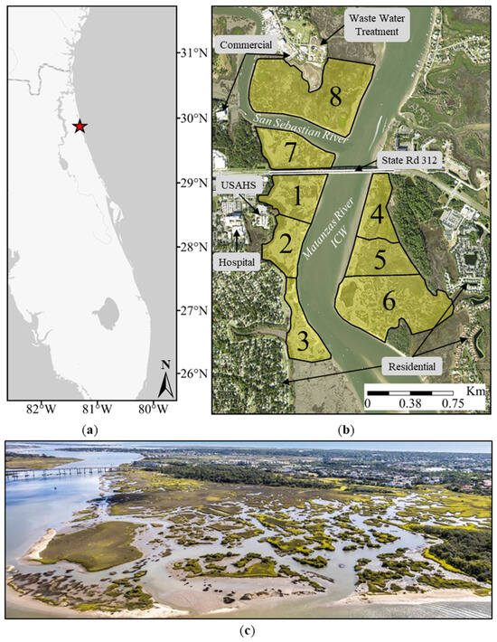
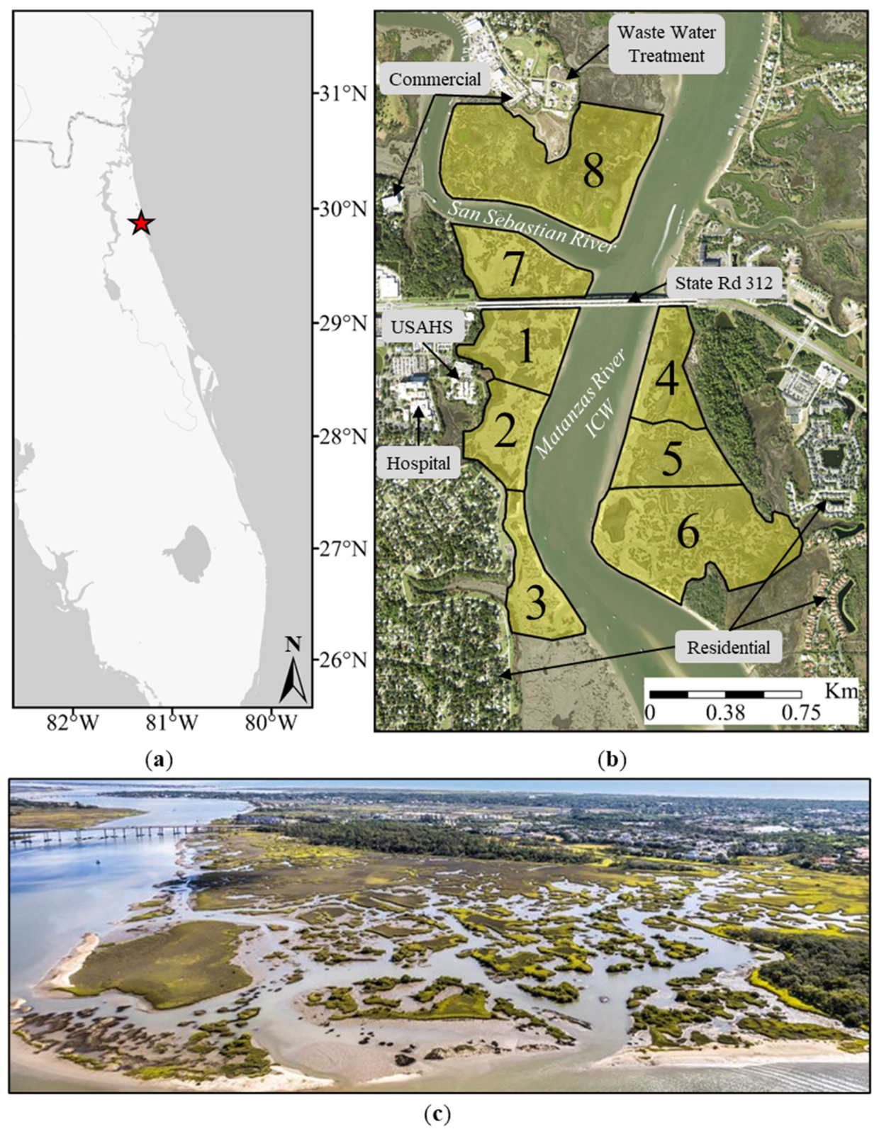
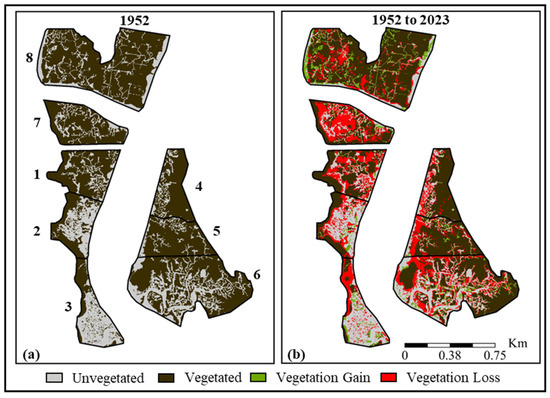
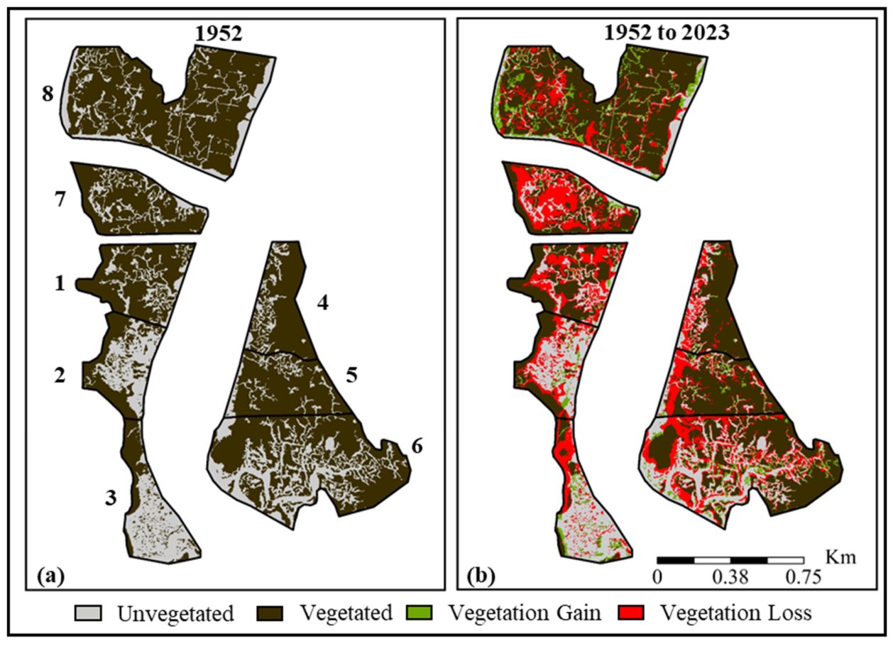
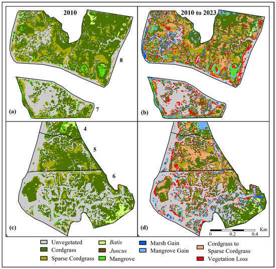
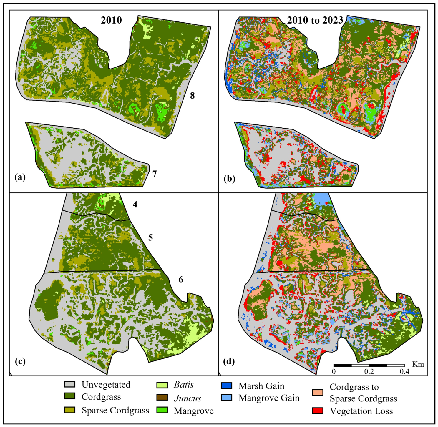
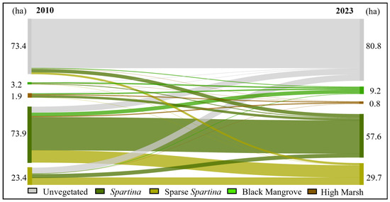
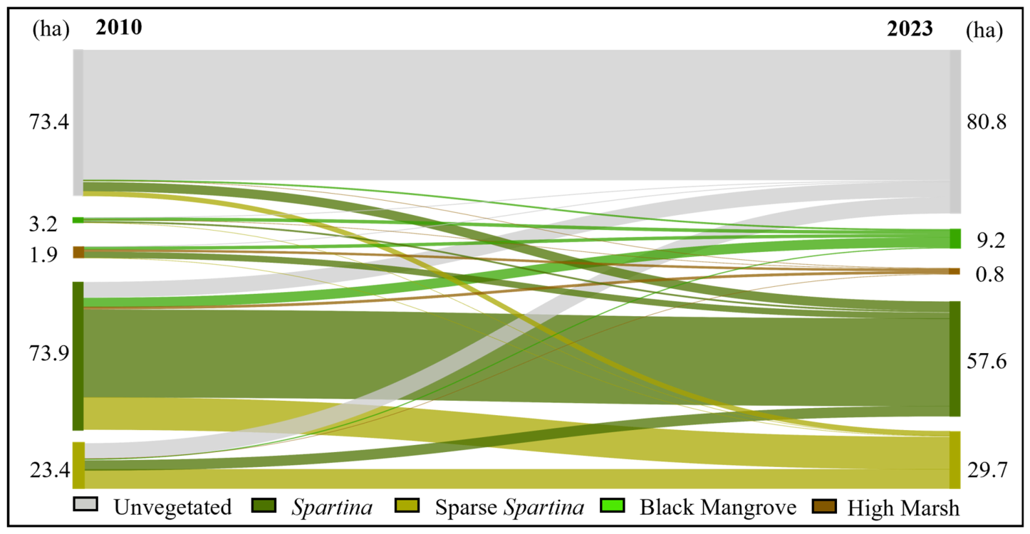
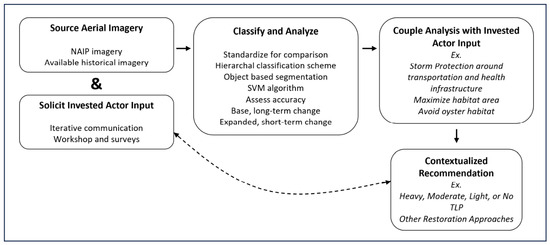
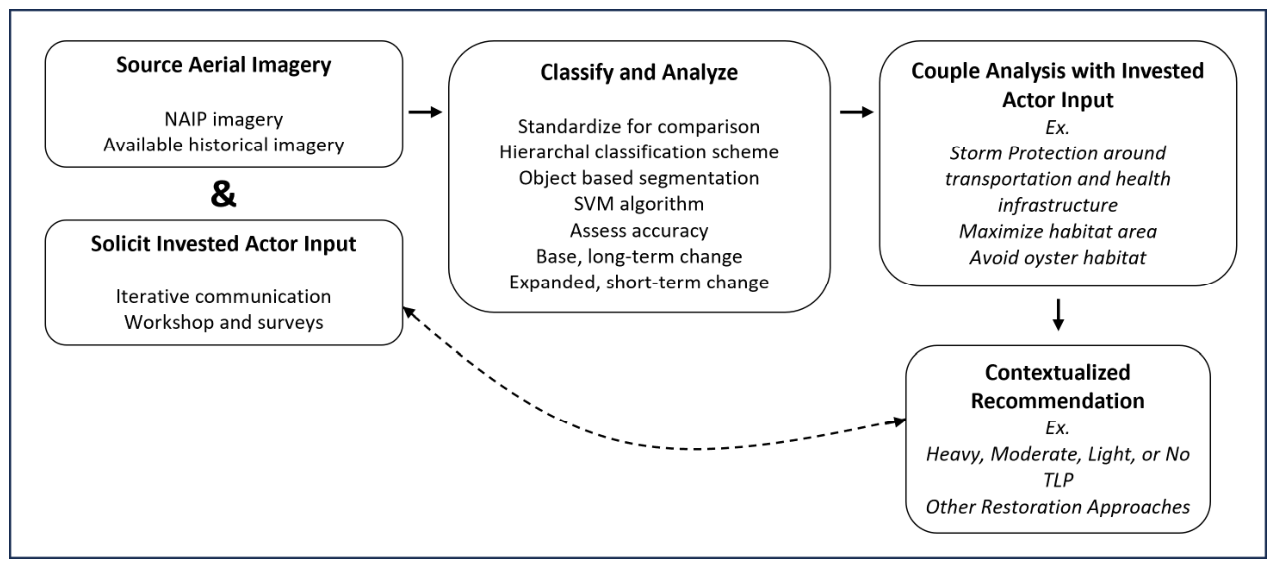

Disclaimer/Publisher’s Note: The statements, opinions and data contained in all publications are solely those of the individual author(s) and contributor(s) and not of MDPI and/or the editor(s). MDPI and/or the editor(s) disclaim responsibility for any injury to people or property resulting from any ideas, methods, instructions or products referred to in the content. |
© 2026 by the authors. Licensee MDPI, Basel, Switzerland. This article is an open access article distributed under the terms and conditions of the Creative Commons Attribution (CC BY) license.