Meteorology-Conditioned High-Resolution Vegetation Forecasting: A Hierarchical Multi-Modal Fusion Network

Highlights

What are the main findings?

• The conditioned reconstruction strategy effectively resolves the resolution mismatch between high-resolution vegetation imagery and coarse meteorological data in mountainous terrain.
• Spectral analysis confirms that the dual-stream encoder autonomously delegates high-frequency spatial reconstruction to NDVI and low-frequency modulation to meteorology.

What are the implications of the main findings?

• Decoupling spatial learning from environmental forcing provides an effective paradigm for fusing multi-resolution remote sensing and climate data.
• The framework supports high-resolution ecological monitoring in topographically complex regions for proactive environmental management.

Abstract

Predicting high-resolution Normalized Difference Vegetation Index (NDVI) in mountainous ecosystems is challenging due to topographic complexity and climate heterogeneity. Existing methods often struggle to balance fine-grained spatial patterns with multi-scale meteorological drivers. This paper introduces the Hierarchical Multi-Modal Fusion Network (HMMFN), which employs a conditioned reconstruction strategy to decouple spatial learning from environmental forcing. The architecture utilizes a dual-stream encoder to process NDVI imagery and meteorological data in parallel. A Transformer module captures long-term temporal dependencies, while a multi-level fusion decoder integrates climate semantics with local vegetation details. The model is optimized using a hybrid loss function that combines Mean Squared Error and Structural Similarity Index Measure to ensure both numerical precision and spatial fidelity. Evaluated in the Liupan Mountains, HMMFN consistently outperforms baseline models across multiple lead times. For prediction horizons ranging from one to five months, the model maintains high accuracy with $R^2$ values between 0.9123 (1-month horizon) and 0.8195 (5-month horizon), achieving a 10.1% and 3.6% reduction in RMSE compared to the optimal baseline model, respectively. These results demonstrate that HMMFN effectively preserves fine-scale spatial structures while maintaining accurate temporal trends across various time steps.

1. Introduction

Vegetation serves as a foundational component of terrestrial ecosystems, critically influencing the global carbon cycle, hydrological balance, and biodiversity [1]. Amidst escalating global climate change, monitoring vegetation dynamics has become a vital indicator of ecosystem health and resilience [2]. The Normalized Difference Vegetation Index (NDVI), derived from satellite remote sensing, provides a robust measure of vegetation density and photosynthetic activity. Its extensive spatial coverage and long-term availability have made it an indispensable tool for applications ranging from agricultural productivity assessment and drought monitoring to ecosystem service evaluation [3,4]. Consequently, the accurate prediction of future NDVI is paramount for proactive environmental management and ecological security assessment.

Recent advancements in artificial intelligence have substantially advanced vegetation dynamics modeling [5,6]. While machine learning models like Random Forest (RF) [7] have shown promise, deep learning architectures such as Convolutional Neural Networks (CNNs) [8] and Long Short-Term Memory (LSTM) networks [9,10,11] have demonstrated notable efficacy. Furthermore, emerging paradigms like QCL-LNF [12] and Reservoir Computing [13] demonstrate the increasing complexity of predictive models. These models are effective at capturing the complex, non-linear relationships between vegetation and climatic drivers [14] and integrating multi-source data to improve predictive accuracy [15]. Most recently, studies in leading journals have highlighted a growing trend toward using advanced multi-modal frameworks to forecast vegetation states under environmental forcing, employing techniques such as transformer-based architectures and spatio-temporal AI approaches [16,17]. However, significant challenges persist, particularly in regions with complex topography and high spatial heterogeneity, such as mountainous ecosystems.

Existing methodologies often face a critical trade-off between temporal depth and spatial fidelity. Models such as LSTMs and Transformers [18,19,20] effectively capture temporal dependencies but frequently require vectorizing spatial information. This process often results in the loss of fine-grained spatial patterns and textures [21]. Conversely, CNN-based approaches are proficient at extracting hierarchical spatial features but may struggle to model long-range temporal dependencies effectively. A further challenge lies in fusing multi-modal data with disparate resolutions. While recent research aims to synthesize cloud-free high-resolution imagery using fusion techniques [17], frameworks that fuse high-resolution NDVI and coarse-resolution meteorological data at early stages often suffer from feature interference or lack mechanisms to adaptively weight distinct information streams [22]. This limitation frequently leads to predictions that, while numerically accurate, exhibit spatial blurring and fail to resolve the boundaries of vegetation patches, hindering local-scale ecological analysis [23]. This highlights the critical necessity for a novel framework capable of decoupling spatial detail retention from temporal trend modeling.

To address these limitations, this paper introduces the Hierarchical Multi-Modal Fusion Network (HMMFN), a novel deep learning framework specifically designed for high-fidelity, long-term NDVI prediction. Our approach moves beyond traditional spatiotemporal fusion, which aims to fill data gaps, and instead focuses on the multi-modal fusion of heterogeneous data: high-resolution vegetation history and coarse-resolution meteorological drivers. This positions HMMFN for crucial application scenarios, including forecasting ecosystem responses to future climate change scenarios and reconstructing historical vegetation dynamics where optical records are missing.

Our study focuses on the Liupan Mountains region, a critical ecological barrier and water source in northwest China. By leveraging historical meteorological patterns to drive future vegetation state forecasting, HMMFN establishes a new paradigm for integrating multi-source data with disparate resolutions. Crucially, the model relies on historical NDVI inputs to provide fine-grained spatial templates (texture and boundaries), while meteorological data provide the temporal forcing signals. The key contributions of HMMFN are the following:

• Decoupled Multi-Scale Feature Extraction: A dual-stream CNN encoder independently processes NDVI and meteorological data. It handles the significant resolution difference through hierarchical feature extraction, ensuring that high-frequency spatial details are preserved from the NDVI stream while meteorological trends are incorporated at appropriate semantic levels.
• Long-Term Temporal Modeling: A Transformer module is employed to effectively capture long-range temporal dependencies and complex lagged responses between climatic factors and vegetation dynamics within annual vegetation cycles, leveraging a 22-year training dataset.
• Hierarchical Multi-Modal Fusion: A multi-level fusion decoder integrates deep temporal context with shallow, high-resolution spatial details. This design ensures that global meteorological trends effectively guide local vegetation reconstruction without blurring essential spatial features.

2. Study Area and Data

2.1. Overview of the Study Area

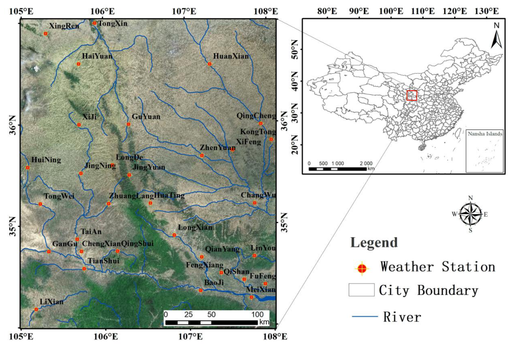
The Liupan Mountains region [24,25], situated at the intersection of Ningxia, Gansu, and Shaanxi provinces, serves as a vital ecological barrier in northwestern China. Geographically, it forms the northern extension of the Qinling Mountains and acts as a natural watershed dividing the Loess Plateau into the Longdong and Longxi regions. The terrain exhibits a narrow north–south orientation with a distinct stepped mountain–hilly landscape, ranging in elevation from 1295 m to 2942 m. Climatically, the region is situated in a critical transitional zone between semi-humid and semi-arid climates, characterized by high sensitivity to environmental forcing and a rich vertical vegetation spectrum, ranging from deciduous broad-leaved forests to subalpine meadows. This complex landscape, combined with significant topographic variability, makes the Liupan Mountains highly representative for studying vegetation–meteorology responses and evaluating the resilience of the northwest ecological barrier. It presents a representative yet challenging environment for testing the robustness of vegetation forecasting models under climatic stress. Importantly, the region is supported by a dense network of high-quality meteorological stations, which provides a unique capacity for the precise verification and calibration of gridded climatic data, a prerequisite for training high-fidelity deep learning frameworks that is often not met in other geographic areas. This study focuses on the core region within coordinates 105°00′–108°00′E and 34°00′–37°00′N, as illustrated in Figure 1.

2.2. Data Sources and Preprocessing

2.2.1. Remote Sensing Data

The NDVI data for this study were sourced from the NASA MOD13Q1 product (https://ladsweb.modaps.eosdis.nasa.gov, 26 January 2026), providing a 22-year time series from January 2001 to December 2022. This product features a 16-day temporal frequency and a 250 m spatial resolution. As an analysis-ready dataset, it has undergone rigorous radiometric calibration and atmospheric correction, making it a widely validated product for monitoring vegetation dynamics [26,27]. Raw data were first reprojected to the WGS84 coordinate system and standardized using the MODIS Reprojection Tools [28]. Subsequently, to mitigate the effects of residual cloud cover and atmospheric noise, this study adopted the Maximum Value Composite (MVC) method [29] to synthesize monthly NDVI from the 16-day MODIS product. The process involves pixel-wise selection of the highest NDVI value within a given month to minimize the influence of transient atmospheric interference. The monthly synthesis is defined as follows:

$$NDV{I}_{month}(i,j)=max\{NDV{I}_1(i,j),NDV{I}_2(i,j),\dots ,NDV{I}_n(i,j)\}$$

(1)

where $NDV{I}_{month}(i,j)$ represents the synthesized NDVI for pixel $(i,j)$, and n denotes the number of 16-day observations within that month (typically $n=2$). Furthermore, a reliability-based filtering was applied prior to synthesis: pixels flagged as “cloud” or “high aerosol” in the MOD13Q1 pixel reliability layer were assigned a zero weight and excluded from the composite. This process, adhering to NASA’s official quality control standards, yielded a total of 505 valid 16-day composites, which were subsequently aggregated into 264 monthly NDVI maps via the MVC method described above.

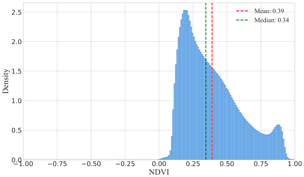
The statistical distribution of NDVI values, calculated from all monthly observations across the entire 2001–2022 dataset (including training, validation, and testing splits), is right-skewed, as shown in Figure 2. The probability density peaks at lower NDVI values, with a mean of 0.39 and a median of 0.34. This distribution characterizes the overall vegetation status of the study area, indicating that coverage is generally moderate, with most NDVI values remaining above 0.

2.2.2. Meteorological Data and Validation

Given the sparse distribution of meteorological stations within the complex terrain of the Liupan Mountains, relying on point-based observations would fail to capture the continuous spatial variation in climate. Therefore, this study utilizes the CN05.1 [30,31] monthly gridded dataset for temperature and precipitation, which has a spatial resolution of 0.25° × 0.25° [32]. This dataset is generated by interpolating data from over 2400 ground stations across China using a thin plate spline method and has been rigorously validated, showing high accuracy and strong correlation with observed measurements [33]. The data spans the same period as the NDVI data (2001–2022).

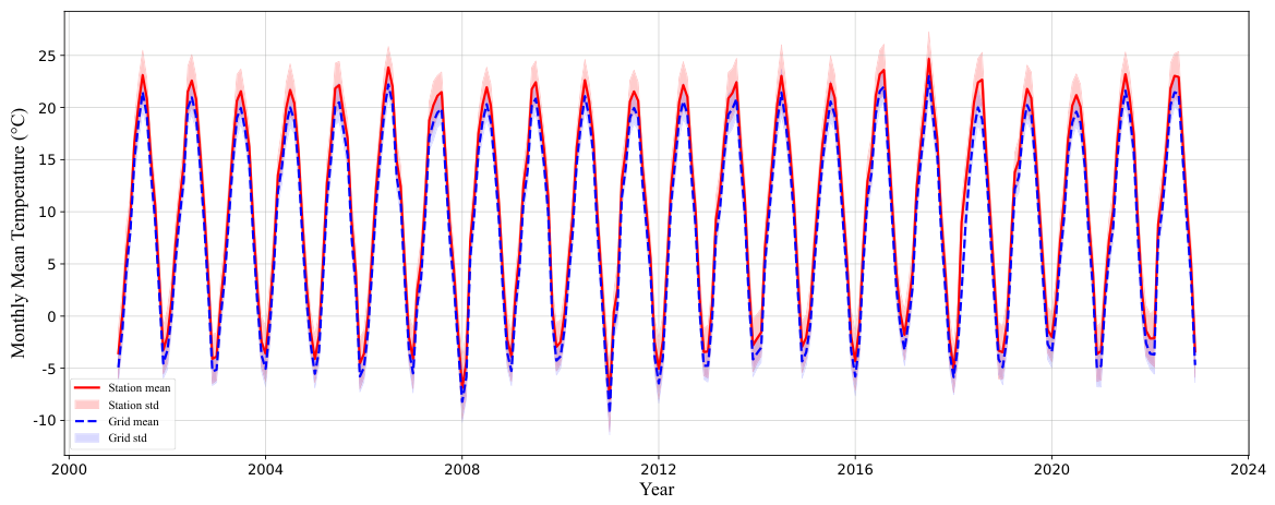
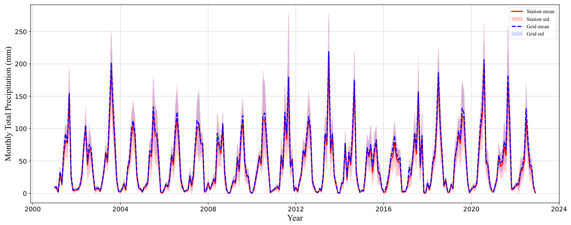
To confirm the dataset’s reliability for our specific region, we compared the gridded data with monthly observations from 32 local ground stations (whose spatial distribution is illustrated in Figure 1). As illustrated in Figure 3 and Figure 4, the validation was performed by comparing the regional mean and standard deviation of the gridded values (sampled at station locations) against the actual station observations. The results demonstrate high consistency and temporal synchronization (blue dashed lines vs. red lines), accurately capturing both the seasonal cycles and inter-annual variability of temperature and precipitation. Despite minor biases arising from the scale difference between point measurements and grid averages, the overall temporal trends are highly synchronized. This high degree of consistency validates the suitability of the CN05.1 dataset as a climatic driver for our predictive model.

2.3. Data Alignment and Multi-Resolution Strategy

A central challenge in this study is the significant resolution discrepancy between the meteorological drivers (∼25 km) and the target NDVI data (250 m). We address this mismatch through a conditioned reconstruction strategy implemented via a dual-stream architecture. First, coarse meteorological grids are resampled to the 250 m NDVI grid using bilinear interpolation to establish pixel-level alignment. This preprocessing step does not synthesize new high-frequency information but provides a spatially registered conditioning field.

The dual-stream encoder then serves as the core feature adaptation mechanism: the NDVI stream extracts and preserves high-resolution spatial templates (textures and boundaries), while the meteorological stream captures broad environmental trends. During the hierarchical fusion process, the model treats the upsampled meteorological data as a conditional forcing signal that modulates the temporal evolution of the spatial patterns derived from historical NDVI. This approach ensures that the resolution limitations of the climate input do not degrade the final spatial fidelity of the vegetation forecast.

3. Methodology

To accurately predict vegetation NDVI dynamics in the complex environment of the Liupan Mountains region, this study proposes a Hierarchical Multi-Modal Fusion Network (HMMFN). The fundamental design philosophy of HMMFN is to address the scale mismatch between drivers and targets by decoupling the learning of spatial patterns (from high-resolution NDVI) and environmental forcing (from coarse-resolution meteorology).

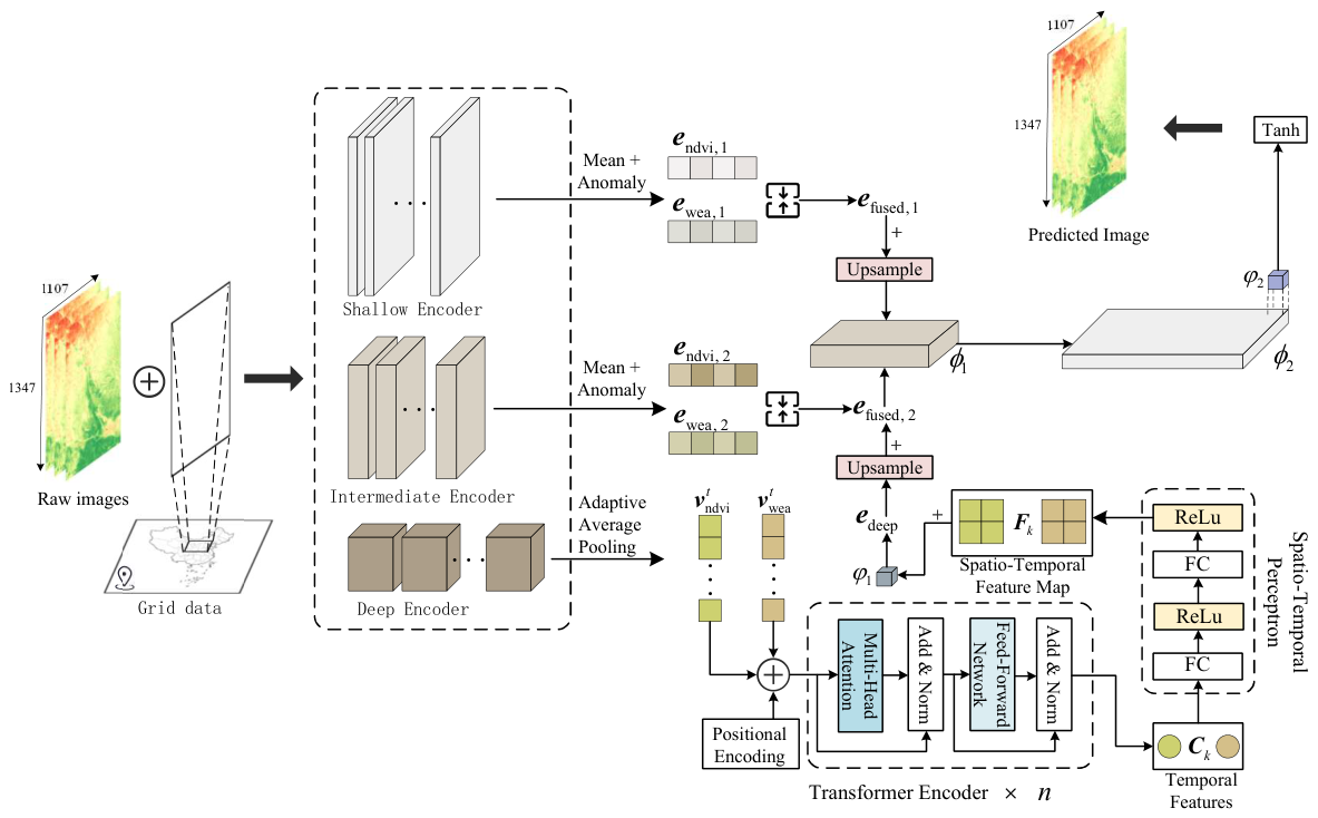
As illustrated in Figure 5, the architecture comprises three integrated components: a Dual-Stream Spatial Feature Encoder, a Transformer-based Temporal Dynamic Modeling module, and a Multi-Level Multi-Modal Fusion Decoder. The model accepts two concurrent time series as input: the NDVI satellite image sequence ${\mathbf{X}}_{\mathrm{ndvi}}\in {\mathbb{R}}^{T\times 1\times H\times W}$ and the corresponding multi-channel meteorological grid data ${\mathbf{X}}_{\mathrm{wea}}\in {\mathbb{R}}^{T\times C\times H\times W}$. Here, T denotes the sequence length, while C, H, and W represent the channels, height, and width, respectively. The objective is to predict the future high-resolution NDVI distribution map $\widehat{\mathbf{Y}}\in {\mathbb{R}}^{1\times H\times W}$ based on the historical evolution over T time steps.

3.1. Dual-Stream Spatial Feature Encoder

To address the significant differences in physical meaning and spatial resolution between NDVI images and meteorological data, an early fusion approach could lead to feature interference and loss of information. Therefore, HMMFN employs a dual-stream design with two independent but structurally identical spatial encoders to process the NDVI and meteorological data separately.

Each encoder consists of three stages designed to extract a hierarchy of spatial features. The NDVI branch uses a single-channel input, while the meteorological branch uses two channels (temperature and precipitation anomalies). In implementation, the encoder adopts three convolutional blocks with a base width of 4 channels. The first block applies a $3\times 3$ convolution with stride 1 and padding 1 to preserve the original spatial resolution while extracting shallow texture features. The second and third blocks use $3\times 3$ convolutions with stride 2 and padding 1 to perform progressive downsampling and expand the channel dimension from $4\to 8\to 16$. Each block is followed by a ReLU activation and batch normalization. For an input sequence of modality $k\in \left\{\mathrm{ndvi},\mathrm{wea}\right\}$, a sample at time step t, denoted as ${\mathbf{x}}_k^t$, is processed by the encoder ${\epsilon }_k$ to yield a set of multi-level feature maps:

$$({\mathbf{e}}_{k,1}^t,{\mathbf{e}}_{k,2}^t,{\mathbf{e}}_{k,3}^t)={\epsilon }_k\left({\mathbf{x}}_k^t\right)$$

(2)

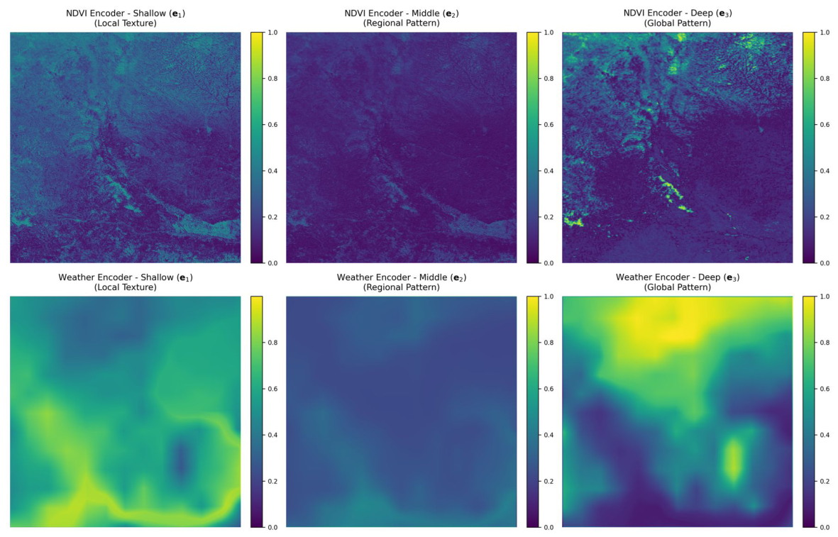
where ${\mathbf{e}}_{k,i}^t$ represents the feature map at level $i\in \{1,2,3\}$. This hierarchical extraction is pivotal for separating information scales. As visualized in Figure 6, the learned representations exhibit distinct semantic roles: the meteorological stream features primarily encode regional gradients and environmental trends. In contrast, the NDVI stream features preserve high-frequency details. Specifically, shallow features ${\mathbf{e}}_{k,1}$ capture local textures and sharp boundaries; intermediate features ${\mathbf{e}}_{k,2}$ represent meso-scale topographic patterns, such as ridges and valleys; and deep features ${\mathbf{e}}_{k,3}$ encapsulate macro-scale geospatial trends. This separation ensures that the high-resolution spatial template is preserved for the decoding phase.

3.2. Temporal Dynamic Dependency Modeling

Vegetation response to climate is non-instantaneous, often exhibiting time lags and cumulative effects [34,35]. To capture these long-term dependencies over the 22-year study period, we employ a Transformer-based temporal encoding module.

First, the deep feature maps ${\mathbf{e}}_{k,3}^t$, which contain the most abstract semantic information, are spatially compressed via global adaptive average pooling to form feature vectors ${\mathbf{v}}_k^t$:

$${\mathbf{v}}_k^t=\mathrm{AdaptiveAvgPool}\left({\mathbf{e}}_{k,3}^t\right)\in {\mathbb{R}}^{C_3}$$

(3)

This transforms the input into a sequence $S_k=[{\mathbf{v}}_k^1,{\mathbf{v}}_k^2,...,{\mathbf{v}}_k^T]\in {\mathbb{R}}^{T\times C_3}$. Since the self-attention mechanism does not inherently encode sequence order, we incorporate sinusoidal positional encoding to preserve temporal information. The positional encoding $\mathrm{PE}\in {\mathbb{R}}^{T\times C_3}$ is defined as:

$$\begin{array}{cc}\hfill & {\mathrm{PE}}_{(pos,2i)}=sin\left(pos/{10000}^{2i/C_3}\right)\hfill \\ \hfill & {\mathrm{PE}}_{(pos,2i+1)}=cos\left(pos/{10000}^{2i/C_3}\right)\hfill \end{array}$$

(4)

where $pos\in [1,T]$ denotes the discrete temporal position in the sequence, $i\in [0,C_3/2-1]$ is the dimension index, and $C_3$ represents the embedding dimension of the deep spatial features. The final input to the Transformer encoder is $S_k^{\prime }=S_k+\mathrm{PE}$.

The sequence $S_k^{\prime }$ is then processed by a multi-head self-attention Transformer encoder. For each attention head, the input sequence is linearly projected into Query ($\mathbf{Q}$), Key ($\mathbf{K}$), and Value ($\mathbf{V}$) matrices:   

$$\mathbf{Q}=S_k^{\prime }{\mathbf{W}}_Q,\mathbf{K}=S_k^{\prime }{\mathbf{W}}_K,\mathbf{V}=S_k^{\prime }{\mathbf{W}}_V$$

(5)

where ${\mathbf{W}}_Q,{\mathbf{W}}_K,{\mathbf{W}}_V\in {\mathbb{R}}^{C_3\times d_k}$ are learnable weight matrices. The self-attention mechanism dynamically computes the correlation between all time steps, allowing the model to weigh the influence of historical climate events on the current vegetation state:

$$\mathrm{Attention}(\mathbf{Q},\mathbf{K},\mathbf{V})=\mathrm{softmax}\left({\displaystyle \frac{\mathbf{Q}{\mathbf{K}}^{\mathrm{T}}}{\sqrt{d_k}}}\right)\mathbf{V}$$

(6)

where $d_k=C_3/h$ represents the dimensionality of the key vectors (with h being the number of attention heads), acting as a scaling factor to prevent the dot product from growing too large and pushing the softmax function into regions with extremely small gradients. The Transformer encoder is configured with $h=4$ attention heads, $L=4$ encoder layers, and a feed-forward dimension of $d_{ff}=64$ ($4\times d$). The input sequence length is $T=12$ months, selected to cover a complete annual vegetation cycle. Fixed sinusoidal positional encoding with a maximum length of 5000 is applied to preserve temporal order without introducing additional learnable parameters. The multi-head outputs are then aggregated along the temporal dimension using mean pooling to produce a final context vector $C_k\in {\mathbb{R}}^{C_3}$, which encapsulates the global temporal dynamics of modality k:

$$C_k={\displaystyle \frac{1}{T}}{\displaystyle \sum _{t=1}^T}\mathrm{TransformerEncoder}{\left(S_k^{\prime }\right)}^t$$

(7)

The hierarchical architecture decouples semantic scales: deep features (${\mathbf{e}}_{k,3}$) capture macro-scale trends and environmental forcing, making spatial compression semantically appropriate, while fine-grained spatial information is preserved through shallow skip connections (${\mathbf{e}}_{k,1}$, ${\mathbf{e}}_{k,2}$). Unlike ViT-based video models that preserve spatial dimensions through spatio-temporal tokens, our pixel-level regression at 337 × 277 resolution would require over 1.1 million tokens per sequence ($O\left(N^2\right)$ complexity), which is computationally infeasible. Empirically, the ablation study in Section 4.4 confirms that replacing the Transformer with temporal average pooling increases the 5-month RMSE by 25.7% and reduces ${\mathrm{R}}^2$ by 11.3%, validating the effectiveness of the compressed temporal representation.

3.3. Hierarchical Multi-Modal Fusion and Decoding

The reconstruction core of HMMFN resides in its decoder, which implements a conditioned reconstruction strategy. Moving beyond simple feature upsampling, the decoder synthesizes global temporal context derived from meteorological data and NDVI history with local spatial details preserved by the NDVI encoder. This integration is facilitated by a multi-level adaptive fusion mechanism embedded within a U-Net-inspired [36] architecture.

3.3.1. Multi-Level Adaptive Fusion

Fusion is performed at multiple semantic levels to ensure that coarse climatic drivers effectively modulate fine-scale vegetation patterns without degrading spatial fidelity. At the deepest level ($i=3$), we synthesize the global trend. The temporal context vectors $C_k$ are projected back to the spatial domain via a Multi-Layer Perceptron (MLP) that maps the temporal features to spatial feature maps:

$${\mathbf{F}}_k=\mathrm{MLP}\left(C_k\right)=\mathrm{ReLU}\left({\mathbf{W}}_2·\mathrm{ReLU}({\mathbf{W}}_1{C}_k+b_1)+b_2\right)\in {\mathbb{R}}^{C_3\times H_3\times W_3}$$

(8)

where ${\mathbf{W}}_1,{\mathbf{W}}_2$ are learnable weight matrices and $b_1,b_2$ are bias terms. This operation broadcasts the global temporal information onto a spatial canvas. The resulting spatio-temporal feature maps from both modalities are then concatenated along the channel dimension and fused through a $1\times 1$ convolution ${\phi }_1$ to form the deep base feature:

$${\mathbf{e}}_{\mathrm{deep}}={\phi }_1({\mathbf{F}}_{\mathrm{ndvi}}\oplus {\mathbf{F}}_{\mathrm{wea}})$$

(9)

where ⊕ denotes channel-wise concatenation. This late-fusion approach ensures that the global environmental forcing signal is established before spatial reconstruction begins.

For the shallower levels $i\in \{1,2\}$, we employ an Adaptive Fusion Block to bridge the gap between historical templates and future predictions. First, an adaptive temporal compression mechanism calculates a representative feature map ${\tilde{\mathbf{e}}}_{k,i}$ by blending the long-term historical mean with the most recent observation, controlled by a learnable scalar parameter ${\lambda }_{st}$ initialized to 0.5:

$${\tilde{\mathbf{e}}}_{k,i}={\lambda }_{st}·\left({\displaystyle \frac{1}{T}}{\displaystyle \sum _{t=1}^T}{\mathbf{e}}_{k,i}^t\right)+(1-{\lambda }_{st})·{\mathbf{e}}_{k,i}^T$$

(10)

This allows the model to dynamically balance the static background landscape (mean) against recent changes (current state).

Subsequently, a cross-modal spatial fusion mechanism integrates these features. For each level i, a learnable scalar weight $w_i$ (initialized to 0.5) determines the fusion ratio through a sigmoid activation:

$${\mathbf{e}}_{\mathrm{fused},i}=\sigma \left(w_i\right)·{\tilde{\mathbf{e}}}_{\mathrm{ndvi},i}+(1-\sigma \left(w_i\right))·{\tilde{\mathbf{e}}}_{\mathrm{wea},i}$$

(11)

where $\sigma (·)=1/(1+e^{-x})$ is the sigmoid function that constrains the weight to the interval $(0,1)$. The gating mechanism integrates high-resolution NDVI textures with meteorological signals. This allows climate data to serve as a condition for modulating regional vegetation patterns during reconstruction.

3.3.2. Decoding and Reconstruction

The final prediction map is progressively reconstructed by upsampling the deep semantic features and concatenating them with the fused skip connections. Starting from ${\mathbf{e}}_{\mathrm{deep}}$, the decoder integrates meso-scale (${\mathbf{e}}_{\mathrm{fused},2}$) and fine-scale (${\mathbf{e}}_{\mathrm{fused},1}$) information through a U-Net-inspired architecture:

$$\begin{array}{cc}\hfill & {\mathbf{d}}_1={\varphi }_1\left({\mathrm{Up}}_1\left({\mathbf{e}}_{\mathrm{deep}}\right)\oplus {\mathbf{e}}_{\mathrm{fused},2}\right)\hfill \\ \hfill & {\mathbf{d}}_2={\varphi }_2\left({\mathrm{Up}}_2\left({\mathbf{d}}_1\right)\oplus {\mathbf{e}}_{\mathrm{fused},1}\right)\hfill \\ \hfill & \mathbf{o}={\phi }_2\left({\mathbf{d}}_2\right)\hfill \end{array}$$

(12)

where ${\mathrm{Up}}_1(·)$ and ${\mathrm{Up}}_2(·)$ denote transposed convolution operations with stride 2 for upsampling, followed by bilinear interpolation for size alignment when necessary. The functions ${\varphi }_1(·)$ and ${\varphi }_2(·)$ are $3\times 3$ convolutional layers with ReLU activation that fuse the upsampled features with the corresponding skip connections via channel-wise concatenation ⊕. Finally, ${\phi }_2(·)$ is a $1\times 1$ convolution that produces the single-channel output. The final output $\mathbf{o}$ is passed through a hyperbolic tangent activation $tanh(·)$ to constrain predictions to the valid NDVI range $[-1,1]$:

$$\widehat{\mathbf{Y}}=tanh\left(\mathbf{o}\right)$$

(13)

3.4. Hybrid Loss Function

To address the common issue of spatial blurring in regression tasks, we optimize HMMFN using a hybrid loss function that balances numerical precision with structural fidelity. The pixel-wise accuracy is enforced by the Mean Squared Error (MSE):

$${\mathcal{L}}_{\mathrm{MSE}}={\displaystyle \frac{1}{HW}}\sum _{h,w}{\left({\widehat{\mathbf{Y}}}_{h,w}-{\mathbf{Y}}_{h,w}\right)}^2$$

(14)

where $\mathbf{Y}$ and $\widehat{\mathbf{Y}}$ denote the ground truth and predicted NDVI maps, respectively, and H, W represent the height and width dimensions. However, compared to standard regression objectives that treat pixels independently and often yield smooth, blurry textures, the Structural Similarity Index Measure (SSIM) explicitly penalizes degradations in local luminance, contrast, and spatial structure. Therefore, we adopt a hybrid of MSE and SSIM to balance numerical precision with structural fidelity:

$$\mathrm{SSIM}(\mathbf{Y},\widehat{\mathbf{Y}})={\displaystyle \frac{(2{\mu }_Y{\mu }_{\widehat{Y}}+C_1)(2{\sigma }_{Y\widehat{Y}}+C_2)}{({\mu }_Y^2+{\mu }_{\widehat{Y}}^2+C_1)({\sigma }_Y^2+{\sigma }_{\widehat{Y}}^2+C_2)}}$$

(15)

where ${\mu }_Y$ and ${\mu }_{\widehat{Y}}$ represent the mean values, ${\sigma }_Y^2$ and ${\sigma }_{\widehat{Y}}^2$ denote the variances, ${\sigma }_{Y\widehat{Y}}$ is the covariance, and $C_1$, $C_2$ are small constants for numerical stability. The total objective function combines both terms:

$$\mathcal{L}={\mathcal{L}}_{\mathrm{MSE}}+\alpha (1-\mathrm{SSIM}(\mathbf{Y},\widehat{\mathbf{Y}}))$$

(16)

where $\alpha$ is a hyperparameter set to 1.0 based on sensitivity analysis. Pure MSE focuses on pixel-wise convergence but fails to penalize degradation of local spatial correlation, often yielding blurry predictions. The SSIM term explicitly preserves structural integrity by penalizing losses in local luminance, contrast, and spatial structure. This hybrid approach balances numerical precision with spatial fidelity, as validated by the ablation study (Section 4.4), where removing SSIM causes SSIM scores to drop by up to 16.2% at the 5-month horizon.

4. Experiments

4.1. Experimental Setup

Baseline models. To rigorously evaluate the performance of HMMFN, we benchmark it against five baseline deep learning models designed for spatio-temporal prediction. To ensure a fair comparison, all baselines receive a unified 3-channel input formed by concatenating single-channel NDVI with two-channel meteorological anomalies along the channel dimension. This early fusion approach allows each model to learn cross-modal interactions through its subsequent convolutional or recurrent layers.

• MM-CNN: A baseline 3D CNN architecture that processes the stacked historical NDVI and meteorological frames to extract joint spatio-temporal features.
• MM-BiRNN: A sequence-to-sequence model that processes flattened multi-modal spatial features through RNN cells to model temporal dynamics.
• MM-LSTM [9]: An advanced recurrent model using Long Short-Term Memory cells to mitigate the vanishing gradient problem and capture longer-term temporal dependencies.
• GWConvLSTM [14]: A geographically weighted ConvLSTM that couples spatial weights with recurrent units via the Hadamard product. It utilizes a spatiotemporal memory flow to dynamically capture local spatial autocorrelation and neighboring contributions during the forecasting process.
• TSD-CNN-LSTM [10]: A hybrid framework that integrates Time Series Decomposition (TSD) with a CNN-LSTM architecture. It decomposes complex NDVI signals into sub-series to better capture the nonlinear responses of vegetation growth to multiple climatic drivers, such as temperature and precipitation.

Evaluation metrics. Model performance was assessed using three standard metrics: Root Mean Square Error (RMSE), Mean Absolute Error (MAE), and the Coefficient of Determination (${\mathrm{R}}^2$).

$$\begin{array}{cc}\hfill & \mathrm{RMSE}=\sqrt{{\displaystyle \frac{1}{n}}\sum _{i=1}^n{(y_i-{\widehat{y}}_i)}^2}\hfill \end{array}$$

(17)

$$\begin{array}{cc}\hfill & \mathrm{MAE}={\displaystyle \frac{1}{n}}{\displaystyle \sum _{i=1}^n}\mid y_i-{\widehat{y}}_i\mid \hfill \end{array}$$

(18)

$$\begin{array}{cc}\hfill & R^2=1-{\displaystyle \frac{{\sum }_{i=1}^n{(y_i-{\widehat{y}}_i)}^2}{{\sum }_{i=1}^n{(y_i-\overline{y})}^2}}\hfill \end{array}$$

(19)

Here, $y_i$ is the ground truth value, ${\widehat{y}}_i$ is the predicted value, $\overline{y}$ is the mean of the ground truth values, and n is the total number of pixels in the test set.

Implementation Details. All models were trained for 100 epochs with the Adam optimizer at an initial learning rate of ${10}^{-3}$ and a weight decay of ${10}^{-5}$. A hybrid MSE-SSIM loss function with data_range $=2.0$ was applied. Learning rate scheduling used ReduceLROnPlateau with a reduction factor of 0.5 and a patience of 10 epochs, combined with gradient clipping at max_norm $=1.0$ and mixed-precision training. All models were implemented in PyTorch 2.0 and trained on an NVIDIA A30 GPU with identical data loading pipelines and evaluation protocols. The base channel multiplier and the number of Transformer layers were both set to 4 based on sensitivity analysis, which indicated that these values balance model capacity with the available training sample size.

Monthly meteorological anomalies were computed by subtracting climatological monthly averages derived from the full 2001–2022 record. This approach follows standard climatological practices in which the baseline represents a stable physical characteristic of the region. Although the test period contributes to these full-period climatological means, the resulting anomaly differences compared to a training-period-only baseline are negligible, with temperature differences of approximately 0.05 °C, indicating no meaningful information leakage. The dataset was chronologically partitioned into training, validation, and independent test sets at an 8:1:1 ratio. The independent test set covers the period from November 2020 to December 2022, providing 26 months of evaluation data. Temporal samples were generated using a 12-month sliding window to predict NDVI at 1-, 3-, and 5-month lead times.

4.2. Quantitative Performance Comparison

We first evaluated the multi-step prediction performance (1, 3, and 5-month horizons) of HMMFN against all baselines. The aggregated quantitative results, presented in

Table 1. Multi-step prediction results on independent test set.

Model	1 Month			3 Months			5 Months
	RMSE	MAE	${\mathbf{R}}^{\mathbf{2}}$	RMSE	MAE	${\mathbf{R}}^{\mathbf{2}}$	RMSE	MAE	${\mathbf{R}}^{\mathbf{2}}$
MM-CNN	0.0898	0.0637	0.8290	0.1291	0.1006	0.6525	0.1640	0.1250	0.4388
MM-BiRNN	0.0985	0.0771	0.7942	0.1229	0.0940	0.6798	0.1563	0.1228	0.4816
MM-LSTM	0.1080	0.0808	0.7527	0.1176	0.0846	0.7067	0.1556	0.1139	0.4946
GWConvLSTM	0.0835	0.0592	0.8520	0.0908	0.0660	0.8280	0.0999	0.0778	0.7881
TSD-CNN-LSTM	0.0715	0.0503	0.8916	0.0898	0.0665	0.8318	0.0956	0.0705	0.8062
HMMFN (Ours)	0.0643 *	0.0455 *	0.9123 *	0.0816 *	0.0560 *	0.8612 *	0.0922 *	0.0671 *	0.8195 *
Improvement (%)	10.07%	9.54%	2.32%	9.13%	15.15%	3.53%	3.56%	4.82%	1.65%

Note: Best results are in bold, second-best in underlined. Improvement (%) is calculated relative to the next-best baseline: $(M_{\mathrm{baseline}}-M_{\mathrm{HMMFN}})/M_{\mathrm{baseline}}\times 100\%$ for RMSE and MAE, and the relative increase for ${\mathrm{R}}^2$. Asterisks denote statistical significance of HMMFN’s improvements over the next-best baseline (* $p<0.01$).

, show that HMMFN achieves higher accuracy than all baseline models across all prediction horizons.

For short-term (1-month) forecasting, HMMFN achieves the lowest RMSE (0.0643) and MAE (0.0455) and the highest ${\mathrm{R}}^2$ (0.9123). It reduces RMSE by approximately 10% compared to the next-best model, TSD-CNN-LSTM. This result suggests that the dual-stream encoder contributes to preserving fine-grained spatial details.

As the prediction horizon extends to 3 and 5 months, all models exhibit a natural decline in performance due to accumulating uncertainty. However, HMMFN demonstrates sustained performance. At the 5-month horizon, where simpler models like MM-CNN and MM-BiRNN experience a severe performance drop, HMMFN maintains a significantly lower RMSE of 0.0922 and a strong ${\mathrm{R}}^2$ of 0.8195. This sustained performance indicates that the Transformer module contributes to capturing long-term temporal dependencies, while the multi-level fusion mechanism helps stabilize predictions over extended horizons.

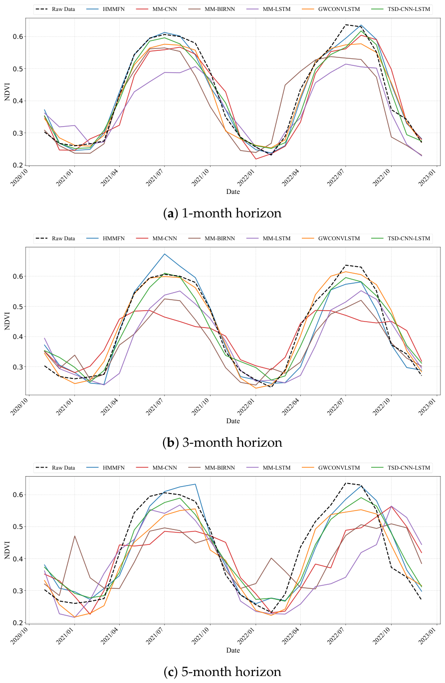
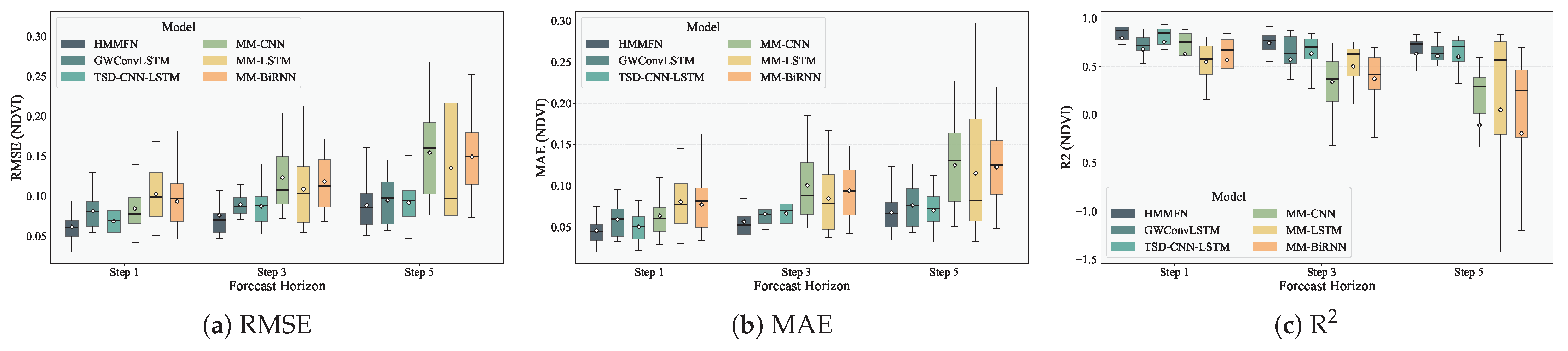
To further analyze these aggregate scores, Figure 7 and Figure 8 present the pixel-level distribution of model performance at each prediction horizon. In Figure 7, HMMFN’s predictions cluster more tightly around the 1:1 line, indicating lower variance and fewer extreme errors. Figure 8 shows that HMMFN yields narrower interquartile ranges along with lower mean and median values for both RMSE and MAE, suggesting relatively stable predictions across diverse spatial and temporal conditions. Paired Wilcoxon signed-rank tests on per-month metrics were performed to assess statistical significance. The 10.01% and 3.56% RMSE improvements at the 1-month and 5-month horizons, respectively, are statistically significant ($p<0.01$), indicating that the observed gains are unlikely to be attributable to random variation.

4.3. Visual and Spatial Fidelity Analysis

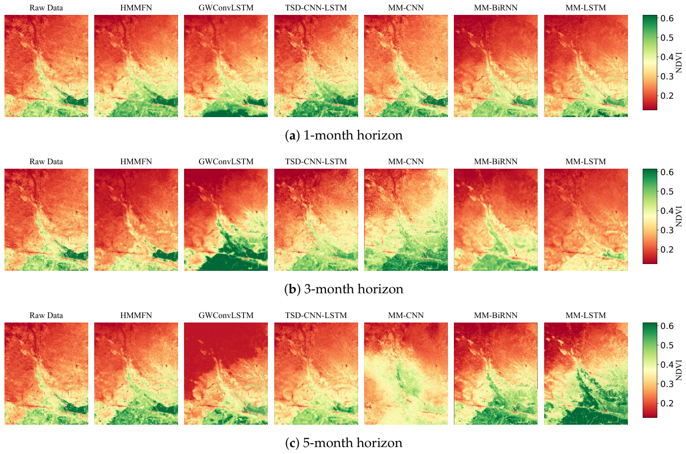
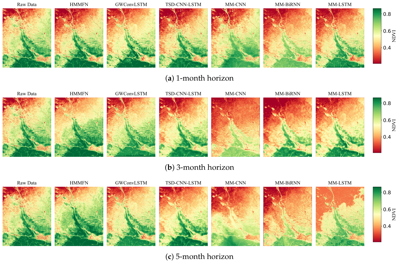
The quantitative performance of HMMFN is visually corroborated by its ability to preserve spatial structure and detail. We analyzed prediction maps for representative months in spring and autumn, as shown in Figure 9 and Figure 10, respectively.

Across all horizons, HMMFN produces predictions that are visually coherent with the ground truth. The model preserves the boundaries of high-vegetation areas along mountain ridges and retains textures in transition zones. The baseline models show different types of degradation: MM-CNN predictions tend to be overly smooth, MM-BiRNN and MM-LSTM struggle to reconstruct sharp spatial gradients due to their flattened sequence processing, and GWConvLSTM shows notable degradation at longer prediction horizons. At the 5-month lead time, baseline models exhibit increased spatial blurring, while HMMFN retains relatively stable spatial coherence.

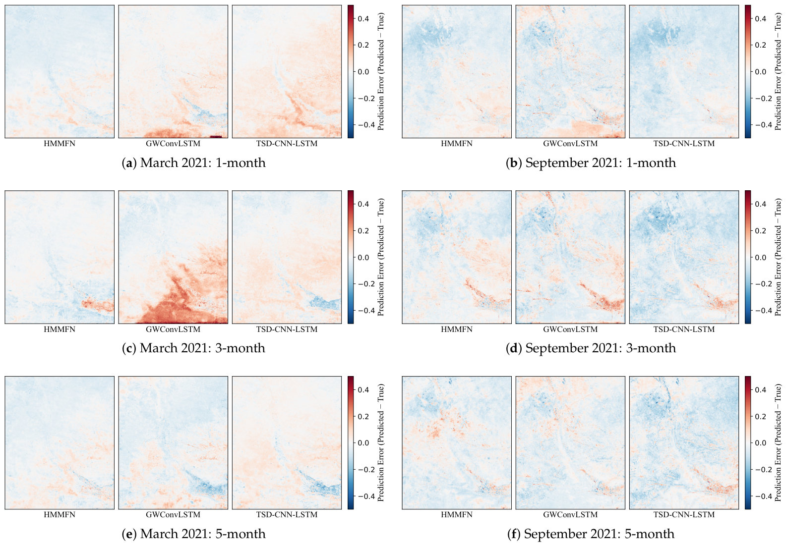
The spatial error maps in Figure 11 further reinforce this analysis. HMMFN displays a relatively uniform error distribution with minimal spatial bias. In contrast, baseline models show region-dependent biases: MM-CNN tends to overestimate NDVI in high-vegetation zones, while MM-BiRNN and MM-LSTM often underestimate it in high-altitude areas. These results suggest that the hierarchical fusion architecture contributes to reducing spatial bias across the diverse topography and climate of the Liupan Mountains.

4.4. Ablation Studies

To evaluate the contribution of each key architectural component of HMMFN, we conducted an ablation study. The results are summarized in

Table 2. Ablation study of model components across multiple time steps.

Model Variant	1 Month			3 Months			5 Months
	RMSE	${\mathbf{R}}^{\mathbf{2}}$	SSIM	RMSE	${\mathbf{R}}^{\mathbf{2}}$	SSIM	RMSE	${\mathbf{R}}^{\mathbf{2}}$	SSIM
w/o Meteorology	0.0785	0.8652	0.8541	0.1050	0.7814	0.7956	0.1254	0.6573	0.7254
w/o Transformer	0.0721	0.8845	0.8923	0.0956	0.8121	0.8317	0.1159	0.7267	0.7824
w/o SSIM Loss	0.0718	0.8751	0.8525	0.0943	0.8257	0.8016	0.1052	0.7938	0.7186
w/o Shallow Fusion	0.0682	0.9015	0.8856	0.0853	0.8547	0.8425	0.0961	0.8052	0.8178
w/o Deep Fusion	0.0754	0.8760	0.8623	0.0983	0.8075	0.8039	0.1156	0.7092	0.7563
w/o NDVI	0.0931	0.7873	0.7885	0.1170	0.6850	0.7498	0.1338	0.6029	0.6920
HMMFN	0.0643	0.9123	0.9180	0.0816	0.8612	0.8852	0.0922	0.8195	0.8574

.

(1) Impact of Meteorological Data (w/o Meteorology): Removing the meteorological input stream resulted in notable performance degradation across all metrics. The 1-month RMSE increased by approximately 22.1% from 0.0643 to 0.0785, while the ${\mathrm{R}}^2$ declined from 0.9123 to 0.8652. This deterioration indicates that, despite their coarse resolution, meteorological variables provide driving information for vegetation dynamics that is not readily captured by historical NDVI sequences alone.

(2) Impact of Temporal Modeling (w/o Transformer): Replacing the Transformer module with temporal average pooling led to a marked performance decline, particularly at longer prediction horizons. The 5-month RMSE increased by 25.7% from 0.0922 to 0.1159, and the ${\mathrm{R}}^2$ declined from 0.8195 to 0.7267. This suggests that explicitly modeling long-term temporal dependencies is important for capturing the lagged responses of vegetation to climatic factors.

(3) Impact of Structural Loss (w/o SSIM Loss): To evaluate the contribution of the structural loss, we trained the model using only MSE loss. This ablation resulted in a significant degradation in structural similarity, with the 1-month SSIM score decreasing from 0.9180 to 0.8525, representing a 7.1% relative decline. The performance gap widens as the prediction horizon extends. At 5 months, the SSIM drops from 0.8574 to 0.7186, a 16.2% decline. This marked reduction indicates that the hybrid loss function plays an important role in mitigating spatial blurring and preserving the structural fidelity of the predictions.

(4) Validation of Hierarchical Fusion (w/o Shallow/Deep Fusion): To validate the necessity of our multi-level fusion design, we conducted two ablations by removing specific fusion pathways while keeping all other components intact. For shallow-level fusion, we removed the fused skip connections $e_{\mathrm{fused},1}$ and $e_{\mathrm{fused},2}$, which combine temporally compressed NDVI and meteorological features. This ablation caused a notable decline in structural similarity: the 1-month SSIM decreased from 0.9180 to 0.8856, a 3.5% drop, and the degradation became more pronounced at longer horizons. These results suggest that shallow-level features contribute to preserving high-frequency spatial details such as textures and boundaries, which support structural integrity. For deep-level fusion, we removed the ${\mathbf{e}}_{\mathrm{deep}}$ feature that integrates temporally aggregated NDVI and meteorological semantics. This ablation primarily affected numerical accuracy: the 1-month RMSE increased from 0.0643 to 0.0754, a 17.3% rise, while the ${\mathrm{R}}^2$ declined from 0.9123 to 0.8760. This suggests that deep features enriched with long-term temporal context contribute to capturing macro-scale geospatial trends relevant to numerical regression accuracy.

(5) Impact of NDVI Spatial Input (w/o NDVI): Removing the NDVI encoder entirely, so that the model relies solely on meteorological data to reconstruct vegetation patterns, resulted in the most severe degradation among all variants. The 1-month RMSE increased by 44.8% from 0.0643 to 0.0931, while the SSIM dropped from 0.9180 to 0.7885, indicating substantial loss of spatial structure. This degradation worsens at longer horizons, with the 5-month ${\mathrm{R}}^2$ declining from 0.8195 to 0.6029. As further confirmed by the spectral analysis in Section 4.7, this condition produces a pronounced decline in high-frequency energy, demonstrating that coarse meteorological data alone is insufficient for synthesizing fine-grained spatial patterns.

To assess the sensitivity of model performance to hyperparameter settings, we evaluated the loss function weight $\alpha$, the base channel multiplier, and the number of Transformer layers, as shown in

Table 3. Sensitivity analysis of hyperparameters and model configurations.

Parameter	Value	1 Month		3 Months		5 Months
		RMSE	${\mathbf{R}}^{\mathbf{2}}$	RMSE	${\mathbf{R}}^{\mathbf{2}}$	RMSE	${\mathbf{R}}^{\mathbf{2}}$
Loss Weight $\alpha$	0.0	0.0718	0.8751	0.0943	0.8257	0.1052	0.7938
	0.5	0.0671	0.8989	0.0855	0.8506	0.0963	0.8112
	1.0	0.0643	0.9123	0.0816	0.8612	0.0922	0.8195
	2.0	0.0658	0.9071	0.0849	0.8489	0.0985	0.8036
Base Channels	2	0.0745	0.8682	0.0958	0.8142	0.1095	0.7618
	4	0.0643	0.9123	0.0816	0.8612	0.0922	0.8195
	8	0.0638	0.9141	0.0825	0.8596	0.0948	0.8132
Transformer Layers	1	0.0702	0.8815	0.0905	0.8332	0.1038	0.7765
	2	0.0671	0.8982	0.0862	0.8485	0.0985	0.7968
	4	0.0643	0.9123	0.0816	0.8612	0.0922	0.8195
	8	0.0665	0.9042	0.0868	0.8425	0.1012	0.7832

Note: Bold values indicate the optimal configuration for each hyperparameter.

. The value $\alpha =1.0$ provides a reasonable balance between numerical precision and structural fidelity: at $\alpha =0$, SSIM decreases from 0.9180 to 0.8525, whereas larger values tend to improve structural similarity at the expense of numerical accuracy. For model capacity, a base multiplier of 4 was found to be the most effective, as larger models exhibit diminishing returns and eventual performance degradation likely due to the limited training sample size. Similarly, a 4-layer Transformer was sufficient to model the multi-scale lagged responses of vegetation to climate without over-fitting.

The complementary nature of the dual-stream design is further examined through spectral pathway analysis and learned fusion weight analysis in Section 4.7, where the results indicate that the two streams operate in distinct frequency domains.

4.5. Spatio-Temporal Correlation Analysis

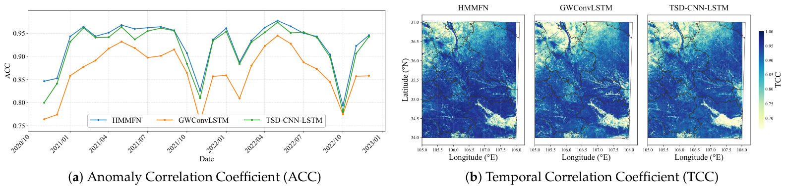
To evaluate HMMFN’s spatio-temporal prediction dynamics, we analyzed the Anomaly Correlation Coefficient (ACC) [37] and Temporal Correlation Coefficient (TCC) [38]. ACC quantifies how accurately the model predicts the spatial pattern of deviations from climatological mean at each time point, while TCC measures the pixel-wise temporal correlation between predicted and observed NDVI sequences throughout the test period.

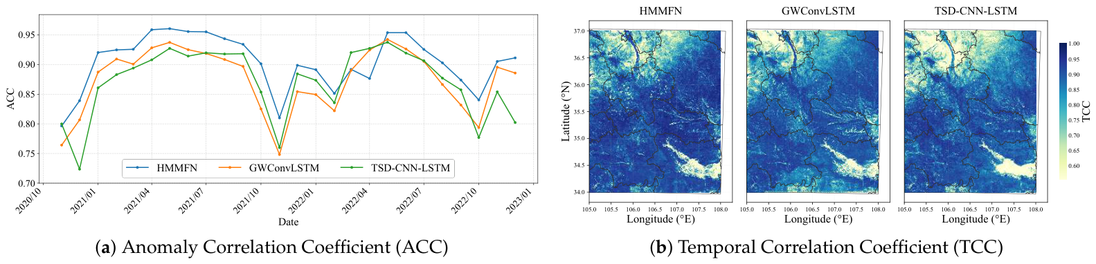
The temporal variations in the ACC for different prediction horizons are illustrated in Figure 12, Figure 13 and Figure 14. HMMFN maintains higher ACC than TSD-CNN-LSTM and GWConvLSTM across all lead times. For the 1-month prediction horizon shown in Figure 12, HMMFN achieves an average ACC of 0.89 and reaches values above 0.95 during the peak growing season. The ACC curves exhibit a clear seasonal periodicity that aligns with the vegetation cycle of the Liupan Mountain region, with higher values observed from May to September.

A significant decrease in predictive accuracy is observed for all models during November of each year. This phenomenon is primarily attributed to the rapid phenological transition in the high-altitude areas of Ningxia. During this period, the vegetation enters a stage of accelerated senescence, which is often accompanied by the onset of snow cover. These environmental factors cause abrupt and non-linear shifts in NDVI values, increasing the difficulty of accurate anomaly capture. HMMFN degrades less during these intervals compared to the baseline models. This advantage suggests that the integration of meteorological variables helps the model track the thermal and hydrological drivers associated with these rapid phenological changes.

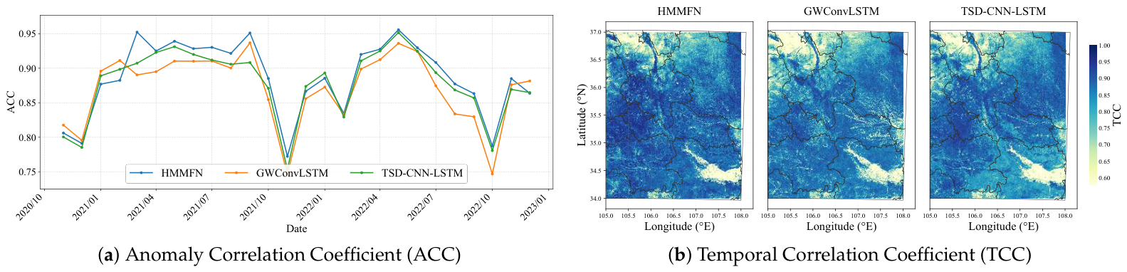
As the prediction horizon extends to 3 months and 5 months, as shown in Figure 13 and Figure 14, all models experience a decline in ACC due to the accumulation of recursive uncertainties and error propagation. Despite this degradation, HMMFN maintains a more stable performance profile than the competing methods. The model effectively preserves the seasonal trajectory even at longer lead times. This sustained accuracy suggests that incorporating climatic forcing enables the model to anticipate seasonal anomalies more effectively than approaches that rely exclusively on historical NDVI patterns.

The spatial heterogeneity of the TCC is presented in the right panels of Figure 12, Figure 13 and Figure 14. For the 1-month prediction horizon, HMMFN shows high TCC values in the center-left portion of the study area. This region corresponds to surfaces where NDVI values remain consistently near zero, suggesting that the model effectively tracks stable land cover signals with minimal temporal variance. A distinct latitudinal gradient is observed in the background NDVI characteristics, with negative NDVI values prevailing in the northern regions and positive values concentrated in the south. HMMFN maintains high predictive accuracy across these diverse ecological zones. In the northern arid and semi-arid sections, the model captures the suppressed vegetation signals. In the southern regions characterized by higher biomass, the model follows the more pronounced seasonal cycles. Compared to the baseline models, TSD-CNN-LSTM and GWConvLSTM show a higher frequency of light-colored patches, particularly in the transitional zones between different NDVI regimes. This indicates that HMMFN reconciles the different temporal dynamics of the arid north and the more vegetated south more effectively.

As the prediction horizon increases to 3 and 5 months, as shown in Figure 13 and Figure 14, the TCC values for all models experience a spatial degradation. The high-correlation zone in the center-left remains the most resilient feature across all lead times. However, HMMFN exhibits a significantly slower rate of accuracy decline in the southern positive-NDVI regions compared to the baselines. This suggests that the integration of meteorological forcing provides essential guidance for predicting vegetation anomalies in areas with high seasonal productivity, even as recursive uncertainties accumulate over longer horizons. The average ACC and TCC values across all models and horizons are summarized in

Table 4. Average ACC and TCC across prediction horizons.

Horizon	Metric	GWConvLSTM	TSD-CNN-LSTM	HMMFN
1-Month	ACC	0.8328	0.8715	0.8942
	TCC	0.8410	0.8842	0.9125
3-Month	ACC	0.8045	0.8310	0.8654
	TCC	0.7915	0.8425	0.8812
5-Month	ACC	0.7712	0.8025	0.8412
	TCC	0.7628	0.8115	0.8540

.

4.6. Computational Efficiency Analysis

Beyond prediction accuracy, computational efficiency is a fundamental requirement for the implementation of deep learning models within operational forecasting frameworks.

Table 5. Computational efficiency comparison of different models for NDVI prediction.

Model	Convergence	Single-Epoch	GPU Memory
	Epochs	Time (s)	Usage (GiB)
MM-CNN	23	31.7	3.2
MM-BiRNN	51	46.2	4.8
MM-LSTM	39	47.8	5.5
GWConvLSTM	57	53.8	9.6
TSD-CNN-LSTM	48	61.4	8.5
HMMFN	61	42.5	8.7

provides a detailed comparison of training convergence characteristics, single-epoch execution durations, and GPU memory utilization for HMMFN and the baseline models. All experiments were performed on a standardized hardware platform equipped with an NVIDIA A30 GPU and an Intel Xeon Silver 4314 CPU. The same training datasets and hyperparameter optimization protocols were applied across all models.

The results indicate that HMMFN achieves a favorable balance between model complexity and execution speed. Among the evaluated architectures, MM-CNN exhibits the lowest computational requirements, involving only 23 convergence epochs and a 3.2 GiB memory footprint. However, this efficiency is associated with a simplified structure that may limit the capacity to capture complex spatiotemporal dependencies. Standard recurrent models, including MM-BiRNN and MM-LSTM, require moderate resources with single-epoch times ranging from 46.2 to 47.8 s and memory usage between 4.8 and 5.5 GiB.

The advanced spatiotemporal baselines, GWConvLSTM and TSD-CNN-LSTM, demonstrate significantly higher computational demands. TSD-CNN-LSTM records the longest single-epoch duration at 61.4 s, while GWConvLSTM reaches the highest peak GPU memory utilization at 9.6 GiB. In contrast, although HMMFN requires 61 epochs to converge, it maintains a relatively high execution efficiency with a single-epoch time of 42.5 s. This is faster than TSD-CNN-LSTM and GWConvLSTM, despite the increased architectural depth of HMMFN. Furthermore, the memory utilization of HMMFN remains at 8.7 GiB, which is approximately 9.4% lower than that of GWConvLSTM.

The efficiency of HMMFN is primarily attributed to its decoupled dual-stream architecture and the integration of parallelized temporal processing modules. Unlike the sequential recurrent operations inherent in GWConvLSTM and TSD-CNN-LSTM, the Transformer-based components within HMMFN leverage the parallel processing capabilities of the A30 GPU more effectively. Additionally, the hierarchical fusion strategy minimizes parameter entanglement by processing meteorological and vegetation signals independently before integration, thereby accelerating the training process [39].

4.7. Information Flow and Diagnostic Analysis

To clarify the internal information flow mechanism and address how high-frequency spatial patterns are preserved while meteorological forcing modulates temporal evolution, we conducted spectral diagnostic analysis on the pathway ablation conditions reported in Table 2. The spectral analysis was performed on a representative subset of the test data to enable 2D Power Spectral Density (PSD) visualization.

4.7.1. Resampling Accuracy Assessment

We first evaluated the fidelity of the bilinear resampling of the CN05.1 meteorological data by comparing the upsampled grids to historical station-based patterns. During the growing season, the resampled temperature exhibited an RMSE of 1.04–1.08 °C with moderate spatial correlation ($r\approx 0.50$–$0.61$), indicating that macroscopic temperature gradients are effectively preserved. During winter, the temperature RMSE increases to approximately 2.33 °C due to terrain-induced microclimates and snow-cover interference. However, for precipitation, the spatial correlation dropped significantly ($r\approx 0.1$–$0.4$) with an RMSE of 16.22–36.28 mm, reflecting the inherent difficulty of capturing fine-scale convective and orographic rainfall patterns within a 25 km grid. These results confirm that the resampling step alone cannot resolve fine-scale meteorological heterogeneity.

However, it is important to emphasize that bilinear resampling serves purely as a dimensional alignment preprocessing step, not as the mechanism for handling the resolution mismatch. The core adaptation is performed by the subsequent dual-stream encoder, which independently extracts high-resolution spatial templates from the NDVI stream and low-frequency environmental trends from the meteorological stream, preventing artificial spatial patterns from propagating into the final prediction. The ablation and spectral analyses below further demonstrate that the network autonomously delegates high-frequency reconstruction to the NDVI stream while restricting resampled meteorological data to deep, low-frequency pathways.

4.7.2. Spectral Pathway Analysis

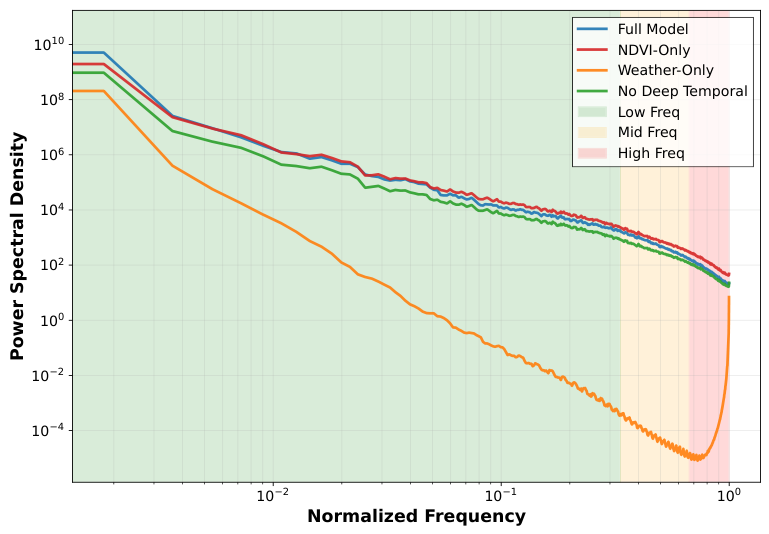
To complement the quantitative ablation results in Table 2 with spectral insights, we analyzed the power spectral density (PSD) of predictions under representative pathway conditions, as shown in Figure 15. The Full Model maintains balanced energy distribution across frequency bands. Removing the meteorological stream (w/o Meteorology) leads to elevated mid-to-high frequency energy, as the model over-replicates historical NDVI patterns without climatic modulation. Conversely, removing the NDVI stream entirely (w/o NDVI) causes a pronounced decline in high-frequency energy, with levels dropping by more than three orders of magnitude in the high-frequency band (>${10}^{-2}$). This confirms that coarse meteorological data alone cannot synthesize fine-grained spatial patterns, supporting the use of NDVI skip connections for spatial fidelity. The w/o Deep Fusion condition preserves spectral shape but loses temporal coherence, suggesting that the deep temporal fusion pathway contributes to time-consistent predictions rather than spatial detail.

Analysis of the trainable fusion gates reveals that at the shallowest level ($e_1$), the model autonomously assigns 62.9% weight to the NDVI stream and 37.1% to the meteorological stream. At the intermediate level ($e_2$), this ratio becomes more balanced (55.8% vs. 44.2%). The temporal aggregation weights are nearly equal (Mean 50.4% vs. Last 49.6%), indicating the model leverages both long-term trends and short-term variations. This hierarchical weighting pattern is consistent with the conditioned reconstruction mechanism, where NDVI contributes more to spatial structure at shallow layers while meteorology’s contribution increases at deeper semantic levels where temporal forcing is integrated.

4.7.3. Pipeline Spectrum Tracing

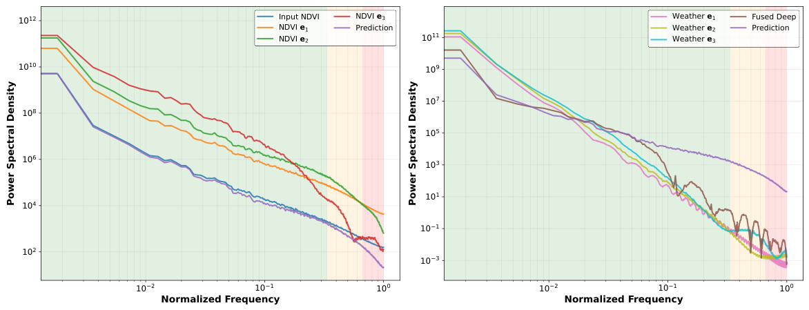
To visualize how spatial energy propagates through the network hierarchy, we tracked the spectral characteristics at each processing stage. Figure 16 presents dual-path spectral evolution.

The input NDVI contains rich high-frequency energy. After passing through the encoder stages (${\mathbf{e}}_1\to {\mathbf{e}}_2\to {\mathbf{e}}_3$), high-frequency energy progressively attenuates due to spatial downsampling. However, the final prediction recovers partial high-frequency energy through skip connections from shallow fused features ($e_{\mathrm{fused},1}$ and $e_{\mathrm{fused},2}$), indicating that the NDVI encoder transmits spatial details to the decoder via these shortcut pathways.

The meteorological encoder stages exhibit rapidly decaying energy with increasing frequency. The Fused Deep representation maintains high energy in the low-frequency band (<${10}^{-1}$) but is substantially lower than the NDVI pathway in the high-frequency band. This suggests that the meteorological pathway primarily contributes low-frequency global trends rather than high-frequency spatial details.

5. Discussion

5.1. Interpretation of Spatiotemporal Mechanisms

The experimental results indicate that HMMFN achieves higher precision in long-term NDVI prediction compared to baseline models. This performance is attributed to the synergistic integration of three mechanisms: (1) meteorological conditioning providing macro-scale temporal drivers; (2) hierarchical fusion balancing regional trends with fine-grained spatial details; and (3) Transformer-based modeling capturing non-linear vegetation-climate lags [40]. As demonstrated by the spectral analysis in Section 4.7, the architecture autonomously delegates high-frequency spatial reconstruction to the NDVI stream at shallow layers while restricting the meteorological pathway to low-frequency temporal modulation. This decoupled processing paradigm has notable implications for vegetation modeling in mountainous ecosystems: it enables the model to maintain the spatial heterogeneity of vegetation patches driven by topographic microclimates, while simultaneously capturing the broader climatic forcing that governs phenological cycles. Such a separation is particularly valuable when meteorological forcing resolution is insufficient to resolve terrain-induced variability—a common constraint in many mountainous regions [23].

5.2. Addressing Scale Mismatch and Heterogeneity

A primary data constraint involves the resolution discrepancy between meteorological drivers (∼25 km) and target NDVI (250 m). Bilinear resampling assumes sub-grid homogeneity, which may omit fine-scale variability driven by topographic effects such as lapse rates and aspect-induced microclimates in the Liupan Mountains. While the dual-stream design mitigates spatial blurring by utilizing high-resolution NDVI skip-connections, localized meteorological events remain partially unrepresented in the forcing signal. Future research could integrate high-resolution digital elevation models (DEM) to derive topographic features as additional conditioning inputs or leverage statistical downscaling techniques to introduce terrain-aware meteorological variability into the coarse-resolution forcing data.

5.3. Error Distribution and Accumulation Mechanisms

Our experimental analysis reveals distinct error distribution rules across different seasons, vegetation types, and prediction durations, highlighting the underlying mechanisms of the model’s performance boundaries.

The predictive performance of HMMFN exhibits seasonal fluctuations that are closely coupled with the fidelity of meteorological drivers and regional phenology. As established in our resampling accuracy analysis in Section 4.7.1, meteorological drivers—particularly temperature—suffer from higher RMSE (∼2.33 °C) during winter due to complex terrain-induced microclimates and snow-cover interference. This data limitation directly propagates to NDVI prediction, where we observe a corresponding accuracy dip in November and December. During these months, the rapid transition of vegetation to senescence, combined with the onset of high-altitude snow, introduces non-linear shifts in the NDVI signal that are difficult to capture through climatic conditioning alone.

In contrast, the model achieves its highest fidelity during the peak growing season (May to September). This period is characterized by high spatial correlation ($r>0.60$) in temperature drivers and robust vegetation-climate responses. Geographically, the southern regions of the Liupan Mountains, which feature high biomass and distinct seasonal cycles, show lower relative errors compared to the northern sparse-vegetation zones. In these arid and semi-arid sections, the dominance of soil background reflectance lowers the signal-to-noise ratio of NDVI observations, making the predictions more susceptible to residual atmospheric noise and background soil moisture fluctuations.

As the prediction lead time extends from 1 to 5 months, error accumulation is driven by two primary mechanisms: recursive uncertainty propagation and low-frequency spectral dominance. In the Transformer module, the attention mechanism must weigh historical observations that are increasingly distant from the target month, weakening the direct causal linkage and leading to a higher variance in the temporal embedding. Simultaneously, while the model’s reliance on high-frequency historical NDVI skip connections remains stable, the precision of the meteorological “modulator” decreases. Since meteorological forcing primarily drives the low-frequency trends (macro-vigor), any variance in the climatic signal compounds over time, leading to a gradual loss of precision in the regional biomass trend while the spatial texture remains relatively sharp. HMMFN mitigates these effects more effectively than baselines by using the conditioned reconstruction strategy to decouple static spatial templates from dynamic temporal forcing, preventing the spatial blurring that typically accompanies recursive error propagation.

5.4. Uncertainty Analysis and Generalization

Diagnostic analysis identifies specific scenarios where prediction uncertainty increases. In high-altitude areas during late autumn (November), snow cover interference can depress NDVI values, introducing signal shifts that are difficult to distinguish from biological senescence within a climate-driven framework. Furthermore, in sparse vegetation zones, soil background interference reduces the signal-to-noise ratio, making the NDVI more sensitive to moisture fluctuations and sun-sensor geometry. Integrating multi-spectral snow indices and soil-adjusted vegetation indices could enhance model robustness in these marginal ecological zones. Additionally, while HMMFN was calibrated using the dense observation network in the Liupan Mountains, its cross-regional generalization requires further empirical verification across diverse climatic regimes and terrains. Although the current model produces deterministic point predictions, incorporating probabilistic frameworks to quantify prediction intervals would enhance its utility for risk-aware applications. The primary challenge lies in the limited training sample size ($N\approx 240$), which makes reliable probabilistic calibration difficult.

6. Conclusions

This study developed the Hierarchical Multi-Modal Fusion Network (HMMFN) for high-resolution NDVI forecasting in mountainous ecosystems. By adopting a conditioned reconstruction strategy, the framework decouples the preservation of fine-scale spatial structure from the integration of coarse-resolution meteorological forcing. Specifically, the dual-stream encoder extracts spatial templates from historical NDVI and environmental signals from meteorological inputs, the Transformer captures long-range temporal dependencies, and the hierarchical fusion decoder reconstructs predictions while maintaining local texture and boundary information.

Experiments in the Liupan Mountains demonstrate that HMMFN consistently outperforms competing baselines across multiple lead times. For prediction horizons from 1 to 5 months, the model maintains strong predictive skill, with $R^2$ values ranging from 0.9123 to 0.8195, while reducing RMSE by 10.01% and 3.56% relative to the best baseline at the 1-month and 5-month horizons, respectively. Ablation and spectral analyses further confirm that meteorological inputs primarily contribute temporal forcing, whereas NDVI pathways are essential for preserving high-frequency spatial details, validating the effectiveness of the proposed hierarchical fusion mechanism.

Despite these encouraging results, prediction accuracy remains constrained by the fidelity of coarse meteorological drivers, especially under winter microclimates and complex precipitation heterogeneity in mountainous terrain. Future work will therefore focus on integrating higher-resolution or terrain-aware meteorological inputs, improving robustness under extreme weather conditions, and evaluating the transferability of the framework across broader ecological regions.

References

1. Xu, L.; Cai, R.; Yu, H.; Du, W.; Chen, Z.; Chen, N. Monthly NDVI Prediction Using Spatial Autocorrelation and Nonlocal Attention Networks. IEEE J. Sel. Top. Appl. Earth Obs. Remote Sens. 2024, 17, 3425–3437. [Google Scholar] [CrossRef]
2. Han, Z.; Li, F.; Zhao, Y.; Liu, C. Investigation into Groundwater Level Prediction within a Deep Learning Framework: Incorporating the Spatial Dynamics of Adjacent Wells. J. Hydrol. 2025, 657, 133097. [Google Scholar] [CrossRef]
3. Mukherjee, J.; Dell’Acqua, F. Influence of Vegetation Features on Corn Yields Estimation Using Different Machine Learning Techniques: A Case Study. In Proceedings of the 2024 IEEE India Geoscience and Remote Sensing Symposium (InGARSS); IEEE: New York, NY, USA, 2024; pp. 1–4. [Google Scholar] [CrossRef]
4. Xu, Q.; Xiao, C.; Zhao, L.; Xing, T.; Wang, L.; Du, Z.; Chen, D.; Liu, P.; Yan, F.; Liu, J.; et al. Diversity of Primary Vegetation Species of Lake Shore Impacts Largely Carbon Emissions in Thermokarst Lakes on the Qinghai-Tibet Plateau. Water Res. 2025, 272, 122946. [Google Scholar] [CrossRef]
5. Prasetya, N.R.; Putra, A.N.; Rayes, M.L.; Utami, S.R. Enhancing Soil Total Nitrogen Prediction in Rice Fields Using Advanced Geo-AI Integration of Remote Sensing Data and Environmental Covariates. Smart Agric. Technol. 2025, 10, 100741. [Google Scholar] [CrossRef]
6. Noa-Yarasca, E.; Osorio Leyton, J.M.; Angerer, J.P. Extending Multi-Output Methods for Long-Term Aboveground Biomass Time Series Forecasting Using Convolutional Neural Networks. Mach. Learn. Knowl. Extr. 2024, 6, 1633–1652. [Google Scholar] [CrossRef]
7. Fu, Y.; Li, R.; Zhu, Z.; Xue, Y.; Ding, H.; Wang, X.; Na, J.; Xia, W. SCARF: A New Algorithm for Continuous Prediction of Biomass Dynamics Using Machine Learning and Landsat Time Series. Remote Sens. Environ. 2024, 314, 114348. [Google Scholar] [CrossRef]
8. Marjani, M.; Mahdianpari, M.; Mohammadimanesh, F. CNN-BiLSTM: A Novel Deep Learning Model for Near-Real-Time Daily Wildfire Spread Prediction. Remote Sens. 2024, 16, 1467. [Google Scholar] [CrossRef]
9. Guo, Y.; Zhang, L.; He, Y.; Cao, S.; Li, H.; Ran, L.; Ding, Y.; Filonchyk, M. LSTM Time Series NDVI Prediction Method Incorporating Climate Elements: A Case Study of Yellow River Basin, China. J. Hydrol. 2024, 629, 130518. [Google Scholar] [CrossRef]
10. Gao, P.; Du, W.; Lei, Q.; Li, J.; Zhang, S.; Li, N. NDVI Forecasting Model Based on the Combination of Time Series Decomposition and CNN–LSTM. Water Resour. Manag. 2023, 37, 1481–1497. [Google Scholar] [CrossRef]
11. Wang, W.; Hu, P.; Yang, Z.; Wang, J.; Zhao, J.; Zeng, Q.; Liu, H.; Yang, Q. Prediction of NDVI Dynamics under Different Ecological Water Supplementation Scenarios Based on a Long Short-Term Memory Network in the Zhalong Wetland, China. J. Hydrol. 2022, 608, 127626. [Google Scholar] [CrossRef]
12. Sun, J.; Shen, J.; Li, H.; Wang, H.; Ren, A.; Zhou, X.; Yong, B. QCL-LNF: A Spatiotemporal Quantum CNN-LSTM Model for Long-Term NDVI Forecasting. IEEE Trans. Geosci. Remote Sens. 2025, 63, 4416914. [Google Scholar] [CrossRef]
13. Olamofe, J.; Ray, R.; Dong, X.; Qian, L. Normalized Difference Vegetation Index Prediction Using Reservoir Computing and Pretrained Language Models. Artif. Intell. Agric. 2025, 15, 116–129. [Google Scholar] [CrossRef]
14. Cai, R.; Xu, L.; Lv, Y.; Wu, T.; Li, X.; Pan, Z.; Yu, H.; Du, W.; Chen, N. Geographically Weighted Convolutional Long Short-Term Memory Neural Networks: A Geospatial Deep Learning Model for Monthly NDVI Prediction. IEEE Trans. Geosci. Remote Sens. 2024, 62, 4415712. [Google Scholar] [CrossRef]
15. Sagan, V.; Maimaitijiang, M.; Bhadra, S.; Maimaitiyiming, M.; Brown, D.R.; Sidike, P.; Fritschi, F.B. Field-Scale Crop Yield Prediction Using Multi-Temporal WorldView-3 and PlanetScope Satellite Data and Deep Learning. ISPRS J. Photogramm. Remote Sens. 2021, 174, 265–281. [Google Scholar] [CrossRef]
16. Farbo, A.; Sarvia, F.; De Petris, S.; Basile, V.; Borgogno-Mondino, E. Forecasting Corn NDVI through AI-based Approaches Using Sentinel 2 Image Time Series. ISPRS J. Photogramm. Remote Sens. 2024, 211, 244–261. [Google Scholar] [CrossRef]
17. Qin, P.; Huang, H.; Chen, P.; Tang, H.; Wang, J.; Chen, S. Reconstructing NDVI Time Series in Cloud-Prone Regions: A Fusion-and-Fit Approach with Deep Learning Residual Constraint. ISPRS J. Photogramm. Remote Sens. 2024, 218, 170–186. [Google Scholar] [CrossRef]
18. Cheng, Y.; Wang, W.; Ren, Z.; Zhao, Y.; Liao, Y.; Ge, Y.; Wang, J.; He, J.; Gu, Y.; Wang, Y.; et al. Multi-Scale Feature Fusion and Transformer Network for Urban Green Space Segmentation from High-Resolution Remote Sensing Images. Int. J. Appl. Earth Obs. Geoinf. 2023, 124, 103514. [Google Scholar] [CrossRef]
19. Hou, H.; Li, R.; Zheng, H.; Tong, C.; Wang, J.; Lu, H.; Wang, G.; Qin, Z.; Wang, W. Regional NDVI Attribution Analysis and Trend Prediction Based on the Informer Model: A Case Study of the Maowusu Sandland. Agronomy 2023, 13, 2882. [Google Scholar] [CrossRef]
20. Benson, V.; Robin, C.; Requena-Mesa, C.; Alonso, L.; Carvalhais, N.; Cortes, J.; Gao, Z.; Linscheid, N.; Weynants, M.; Reichstein, M. Multi-Modal Learning for Geospatial Vegetation Forecasting. In Proceedings of the 2024 IEEE/CVF Conference on Computer Vision and Pattern Recognition (CVPR), Seattle, WA, USA, 16–22 June 2024; IEEE: New York, NY, USA, 2024; pp. 27788–27799. [Google Scholar] [CrossRef]
21. Cui, C.; Zhang, W.; Hong, Z.; Meng, L. Forecasting NDVI in Multiple Complex Areas Using Neural Network Techniques Combined Feature Engineering. Int. J. Digit. Earth 2020, 13, 1733–1749. [Google Scholar] [CrossRef]
22. Wang, Y.; Zhang, N.; Chen, M.; Zhao, Y.; Guo, F.; Huang, J.; Peng, D.; Wang, X. Prediction and Spatiotemporal Dynamics of Vegetation Index Based on Deep Learning and Environmental Factors in the Yangtze River Basin. Forests 2025, 16, 460. [Google Scholar] [CrossRef]
23. Maselli, F.; Chiesi, M.; Pieri, M. A New Method to Enhance the Spatial Features of Multitemporal NDVI Image Series. IEEE Trans. Geosci. Remote Sens. 2019, 57, 4967–4979. [Google Scholar] [CrossRef]
24. Lin, T.; Shu, Z.; Deng, P.; Tian, L.; Sun, Y.; Jia, L.; Cao, N.; Bai, H. Vertical Distribution of Different Phase Particles in Summer Topographic Clouds over Liupan Mountain. Phys. Chem. Earth Parts A/B/C 2026, 142, 104212. [Google Scholar] [CrossRef]
25. Li, Y.; Zhang, S.; Liu, D.; Zhang, T.; Zhang, Z.; Zhao, J.; Zhang, B.; Cao, S.; Xu, X.; Yao, Q.; et al. Migration of Wheat Stripe Rust from the Primary Oversummering Region to Neighboring Regions in China. Commun. Biol. 2025, 8, 350. [Google Scholar] [CrossRef] [PubMed]
26. Jiang, W.; Yuan, L.; Wang, W.; Cao, R.; Zhang, Y.; Shen, W. Spatio-Temporal Analysis of Vegetation Variation in the Yellow River Basin. Ecol. Indic. 2015, 51, 117–126. [Google Scholar] [CrossRef]
27. Jia, Z.; Zhang, Z.; Cheng, Y.; Buhebaoyin; Borjigin, S.; Quan, Z. Grassland Biomass Spatiotemporal Patterns and Response to Climate Change in Eastern Inner Mongolia Based on XGBoost Model Estimates. Ecol. Indic. 2024, 158, 111554. [Google Scholar] [CrossRef]
28. Htway, N.N.; Thin, L.M. Prediction of Land Surface Temperature in Dry Zone, Myanmar Using MODIS Derived NDVI and LST. In Proceedings of the 2024 IEEE Conference on Computer Applications (ICCA); IEEE: New York, NY, USA, 2024; pp. 1–6. [Google Scholar] [CrossRef]
29. Ramirez-Gonzalez, D.A.; Chokmani, K.; Cambouris, A.N.; D’Souza, M.L. Delineation of Management Zones Based on the Agricultural Potential Concept for Potato Production Using Optical Satellite Images. Remote Sens. 2025, 17, 3709. [Google Scholar] [CrossRef]
30. Yang, C.; Li, X.; Zhang, X.; Wu, J.; Li, L. Evaluation and comparison of separated precipitation types from multi-sources data in the Chinese Tianshan mountainous region. J. Mt. Sci. 2025, 22, 489–504. [Google Scholar] [CrossRef]
31. Hu, Y.; Li, H.; Zhang, C.; Shen, D.; Xu, B.; Chen, M.; Chu, W.; Li, R. Exploring Diverse Modeling Schemes for Runoff Prediction: An Application to 544 Basins in China. EGUsphere 2025, 2025, 1–51. [Google Scholar] [CrossRef]
32. Wu, J.; Gao, X.; Giorgi, F.; Chen, D. Changes of Effective Temperature and Cold/Hot Days in Late Decades over China Based on a High Resolution Gridded Observation Dataset. Int. J. Climatol. 2017, 37, 788–800. [Google Scholar] [CrossRef]
33. Zhu, Y.Y.; Yang, S. Evaluation of CMIP6 for Historical Temperature and Precipitation over the Tibetan Plateau and Its Comparison with CMIP5. Adv. Clim. Chang. Res. 2020, 11, 239–251. [Google Scholar] [CrossRef]
34. Huang, M.; Lu, R.; Zhang, Z.; Zhou, Y.; Li, P.; Du, P.; Zhao, T.; Xiao, S. Fine-scale analysis of the cumulative and time-lagged effects of drought on vegetation in the Ili River Basin, Central Asia. J. Environ. Manag. 2025, 392, 126670. [Google Scholar] [CrossRef] [PubMed]
35. Wang, C.; Chen, J.; Lee, S.C.; Xiong, L.; Su, T.; Lin, Q.; Xu, C.Y. Response and recovery times of vegetation productivity under drought stress: Dominant factors and relationships. J. Hydrol. 2025, 655, 132945. [Google Scholar] [CrossRef]
36. Lin, N.; Quan, H.; He, J.; Li, S.; Xiao, M.; Wang, B.; Chen, T.; Dai, X.; Pan, J.; Li, N. Urban vegetation extraction from high-resolution remote sensing imagery on SD-UNet and vegetation spectral features. Remote Sens. 2023, 15, 4488. [Google Scholar] [CrossRef]
37. Wang, T.; Ma, S.; Zhu, C. Distinct response of summer rainfall anomalies over East Asia to the interannual variability of the annual cycle of East Asian summer monsoon. J. Clim. 2026, 39, 1279–1294. [Google Scholar] [CrossRef]
38. Dastigerdi, M.; Nadi, M.; Mashhadi, B.S.; Serrano-Notivoli, R. Analyzing vegetation dynamics and climate variability in the western Caspian ecosystem using MODIS NDVI time series data. Geosyst. Geoenviron. 2026, 100491. [Google Scholar] [CrossRef]
39. Lykhovyd, P.; Lavrenko, S.; Lavrenko, N.; Revto, O.; Maliarchuk, A.; Maliarchuk, V. Comparative Performance of ANN Predicting Soybean Yields from NDVI: Execution Time and CPU Usage in C and Python. In Proceedings of the 2025 15th International Conference on Advanced Computer Information Technologies (ACIT); IEEE: New York, NY, USA, 2025; pp. 902–905. [Google Scholar] [CrossRef]
40. Blanc-Betes, E.; Welker, J.M.; Gomez-Casanovas, N.; DeLucia, E.H.; Peñuelas, J.; de Oliveira, E.D.; Gonzalez-Meler, M.A. Strong Legacies of Emerging Trends in Winter Precipitation on the Carbon-Climate Feedback from Arctic Tundra. Sci. Total Environ. 2025, 962, 178246. [Google Scholar] [CrossRef]
Figure 1. Location of the Liupan Mountains region, showing its geographical context and the distribution of surrounding weather stations.
Remotesensing 18 01684 g001
Figure 2. Probability distribution of MODIS NDVI data (2001–2022) for the Liupan Mountains region, computed from all monthly observations in the complete dataset. The distribution reflects the area’s predominantly moderate vegetation cover.
Remotesensing 18 01684 g002
Figure 3. Comparison of monthly mean temperature between the CN05.1 gridded dataset and ground station observations. The strong alignment in seasonality and trends confirms the gridded data’s validity.
Remotesensing 18 01684 g003
Figure 4. Comparison of monthly mean precipitation between the CN05.1 gridded dataset and ground station observations. The consistency in capturing seasonal peaks and variability supports its use as a model driver.
Remotesensing 18 01684 g004
Figure 5. The overall architecture of the Hierarchical Multi-Modal Fusion Network (HMMFN), illustrating the dual-stream encoding, temporal dependency modeling, and multi-level fusion decoding process.
Remotesensing 18 01684 g005
Figure 6. Visualization of learned feature representations from the dual-stream encoder. The top row shows NDVI features, and the bottom row shows meteorological features. Columns correspond to shallow ( e 1 , Local Texture), intermediate ( e 2 , Regional Pattern), and deep ( e 3 , Global Pattern) levels, confirming the hierarchical extraction of geographically meaningful patterns.
Remotesensing 18 01684 g006
Figure 7. Pixel-level performance comparison across all models at different prediction horizons. Metrics are computed by flattening predicted and ground truth NDVI images and calculating RMSE, MAE, and R 2 for each test sample.
Remotesensing 18 01684 g007
Figure 8. Distribution of prediction errors across all test samples for different models. The box plots show the median (center line), average (diamond shape) and interquartile range (box) for each evaluation metric.
Remotesensing 18 01684 g008
Figure 9. Visual comparison of model predictions for March 2021 across different prediction horizons.
Remotesensing 18 01684 g009
Figure 10. Visual comparison of model predictions for September 2021 across different prediction horizons.
Remotesensing 18 01684 g010
Figure 11. Spatial error distribution of model predictions across different dates and prediction horizons. Red areas indicate overestimation, blue areas indicate underestimation, and white represents minimal error. (a,b) 1-month horizon; (c,d) 3-month horizon; (e,f) 5-month horizon.
Remotesensing 18 01684 g011
Figure 12. Spatio-temporal correlation analysis for 1-month prediction horizon.
Remotesensing 18 01684 g012
Figure 13. Spatio-temporal correlation analysis for 3-month prediction horizon.
Remotesensing 18 01684 g013
Figure 14. Spatio-temporal correlation analysis for 5-month prediction horizon.
Remotesensing 18 01684 g014
Figure 15. Spectral analysis of representative pathway ablation conditions from Table 2. The power spectral density (PSD) of predictions is compared across normalized frequency bands. The Full Model maintains balanced energy distribution, w/o Meteorology exhibits elevated mid-to-high frequency energy due to over-replication of historical patterns, w/o NDVI shows a pronounced decline in high-frequency energy, and w/o Deep Fusion preserves spectral shape but loses temporal coherence.
Remotesensing 18 01684 g015
Figure 16. Spectral energy flow through the HMMFN pipeline. Left: NDVI pathway showing energy propagation from input through encoder stages ( e 1 , e 2 , e 3 ) to final prediction. Right: Meteorological pathway showing energy distribution in encoder stages and fused deep features. Shaded regions indicate low-frequency (green), mid-frequency (yellow), and high-frequency (red) bands.
Remotesensing 18 01684 g016