Hyperspectral Image Change Detection with Deep Learning: Methods, Trends, and Challenges

Highlights

What are the main findings?

• The review identifies deep neural architectures as the dominant paradigm in hyperspectral image change detection, particularly because of their ability to jointly encode spectral correlation, spatial structure, and temporal discrepancy information in complex high-dimensional scenes.
• It also shows that recent advances are increasingly centered on hybrid and label-efficient learning strategies, including CNN transformer, CNN + GCN, and self-/semi-supervised frameworks, to address annotation scarcity and improve robustness.

What are the implications of the main findings?

• These findings indicate that future progress in hyperspectral change detection will depend on unifying spectral modeling, spatial-context reasoning, and temporal representation learning within data-efficient architectures that remain robust to domain shifts, spectral variability, and limited supervision.
• The review also highlights the need for standardized benchmarks, more rigorous evaluation protocols, and computationally efficient yet interpretable models to support reproducible research and facilitate operational deployment in real-world remote sensing applications.

Abstract

Hyperspectral image change detection (HSI-CD) is becoming increasingly important in understanding how the Earth’s surface evolves over time, from monitoring ecosystems to tracking urban expansion. Unlike traditional pixel-based or hand-crafted approaches, deep learning models can automatically learn powerful spectral–spatial features, making them especially effective for this task. In this review, we bring together recent advances in deep learning for HSI-CD, combining a meta-analysis of the literature with an overview of the main model families and training strategies. We cover supervised, semi-supervised, and unsupervised methods, as well as newer directions such as transfer learning, self-supervised frameworks, and hybrid designs that blend CNNs, transformers, and graph neural networks. We also discuss benchmark datasets, evaluation protocols, and case studies that show how these methods perform in practice. Beyond summarizing the current progress, the review highlights ongoing gaps, such as limited labeled data, generalization across sensors, computational efficiency, and the need for interpretability, and points to emerging opportunities for future work. Our goal is to provide both a snapshot of the current state of the field and a road map for advancing deep learning-based HSI-CD.

1. Introduction

Deep Learning (DL) is rapidly becoming a dominant area in big data analysis, with an increase in the deployment of remote sensors and image acquisition in recent years. DL has emerged as a powerful paradigm due to its ability to learn complex hierarchical feature representations directly from raw hyperspectral data. As a subfield of machine learning (ML), DL is inspired by the structure and functioning of the biological brain [1,2]. DL-based models are typically implemented using artificial neural networks (ANNs) [3], characterized by their layered architectures composed of interconnected computational units (neurons). As remote sensing technologies continue to evolve, it becomes easier to gather varied images through multiple sensors, enhancing our capability to study the Earth’s surface. The increased availability of remote sensing hyperspectral images (HSIs) provides an important and unique data source for Earth observation (EO). HS images are characterized by detailed spectral sampling (i.e., very high spectral resolution) over a wide spectral wavelength range, which makes it possible to monitor land-cover dynamics at a fine spectral scale. This is due to its capability to detect subtle spectral variations in multitemporal images associated with land-cover changes that are not detectable in traditional multispectral images (MSIs) because of their limited spectral resolution (i.e., sufficient for representing only abrupt, strong changes in the spectral signature, as a rule). To fully exploit the available multitemporal HS images and their rich information content in change detection (CD), it is necessary to develop advanced automatic techniques that can address the complexity of extracting change information in an HS space. This article provides a comprehensive overview of the CD problem in HSIs, as well as a survey of the main CD techniques available for multitemporal HS images. Therefore, this review centers on investigating DL techniques for change detection utilizing HS images.

Many change detection researchers have developed several techniques over the past few decades. Prior to deep learning, pixel-based classification techniques showed significant progress [4,5,6,7]. The majority of conventional methods concentrated on detecting altered pixels and categorizing them to produce change maps. These techniques often had accuracy and generalization issues even though they performed well on some image types. Additionally, the threshold parameters and classifiers they employed affected their performance [8]. At the same time, advances in satellite and airborne sensors completely changed the landscape. Today, we have instruments that can capture hyperspectral data at massive scales, sometimes gigabytes or even terabytes per hour. This creates both an opportunity and a challenge. The data are rich and full of detail, but they are also high-dimensional and complex, making it hard for traditional methods to keep up. Older algorithms struggle with the so-called “curse of dimensionality” and simply cannot take full advantage of the rich spectral–spatial information now available. Deep learning has stepped in as a natural fit for this new era. With its ability to automatically learn spectral–spatial representations from large datasets, it has rapidly outperformed conventional methods and become the dominant direction for HSI-CD. In this review, we specifically focus on the intersection of hyperspectral imagery and deep learning for change detection, highlighting how different architectures, strategies, and supervision levels have been applied to this problem.

The remainder of the paper is structured as follows. Section 2 presents a meta-analysis of the recent literature on HSI-CD, synthesizing key findings and research directions. Section 3 provides a background on hyperspectral imaging and change detection and discusses trends and challenges of applying deep learning in this domain. Section 4 surveys the architectural landscape of deep learning approaches, while Section 5 reviews the learning strategies adopted to enhance model performance and generalization. Section 6 outlines the evaluation protocols commonly used in HSI-CD research. Section 7 introduces benchmark datasets and selected case studies. Section 8 offers a discussion of the gaps in research and future direction. Finally, Section 9 concludes the paper with key insights.

2. Meta-Analysis of Recent Literature in HSI-CD

A bibliometric and quantitative meta-analysis allows us to take a broader perspective on the overall development of the field. This examination goes beyond individual method descriptions and provides a broader view of how deep learning-based hyperspectral image change detection (HSI-CD) has evolved over time. In particular, it helps reveal not only the steady growth in research activity, but also the architectural preferences and methodological directions that have shaped the field in recent years.

Search Strategy and Study Selection

To provide a reproducible basis for the meta-analysis, the literature search was conducted in the Web of Science (WoS) Core Collection using the Topic field (TS). The search targeted publications from 2018 to 2025 and was designed to capture studies at the intersection of deep learning, hyperspectral imagery, and change detection. The search was restricted to the publication years 2018–2025 and was performed across the relevant WoS indexes considered in this review. Both peer-reviewed journal articles and indexed conference papers, including relevant IEEE conference publications, were considered in the initial retrieval stage. After the initial retrieval, duplicate and clearly irrelevant records were removed. The remaining papers were screened based on title, abstract, and, where necessary, full-text review. A study was included in the final meta-analysis if it adhered to the following: (1) focused on hyperspectral image change detection; (2) used deep learning as a primary methodological component; and (3) reported a method, framework, or experimental evaluation directly relevant to HSI-CD. Papers were excluded if they (1) focused on multispectral, SAR, or other remote sensing change detection tasks without a hyperspectral component; (2) addressed hyperspectral classification, segmentation, restoration, or related tasks without change detection; or (3) lacked sufficient methodological relevance to the scope of this review.

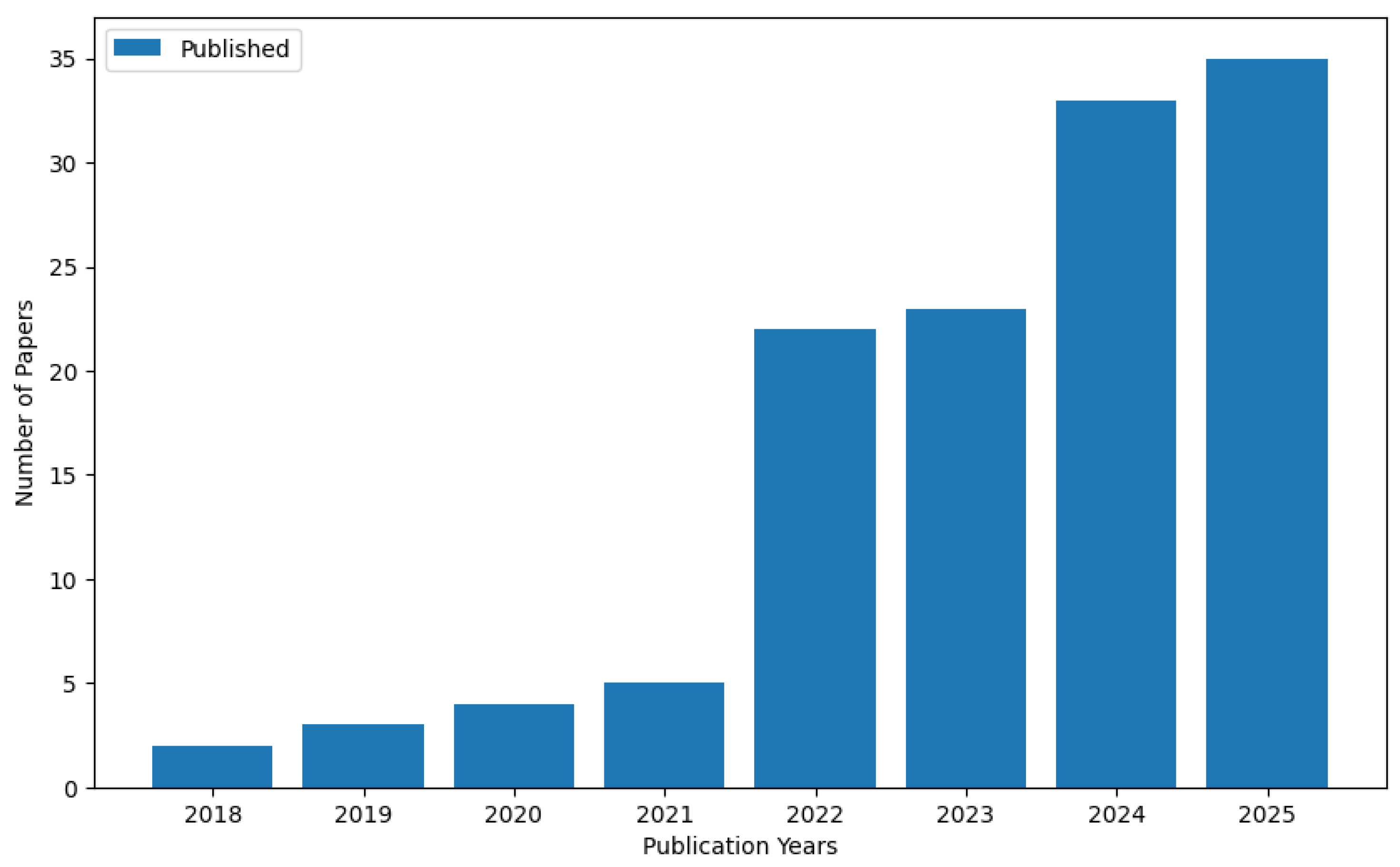
Figure 1 illustrates the annual number of publications on deep learning-based HSI-CD between 2018 and 2025. Based on the final screened set of studies, the figure shows a progressive increase in research activity over time. The trend reflects an early adoption phase in 2018–2019, a steady rise during 2020–2021, and a more pronounced increase from 2022 onward. This pattern highlights the growing interest in applying deep learning techniques to hyperspectral change detection and confirms the rapid expansion of the field in recent years.

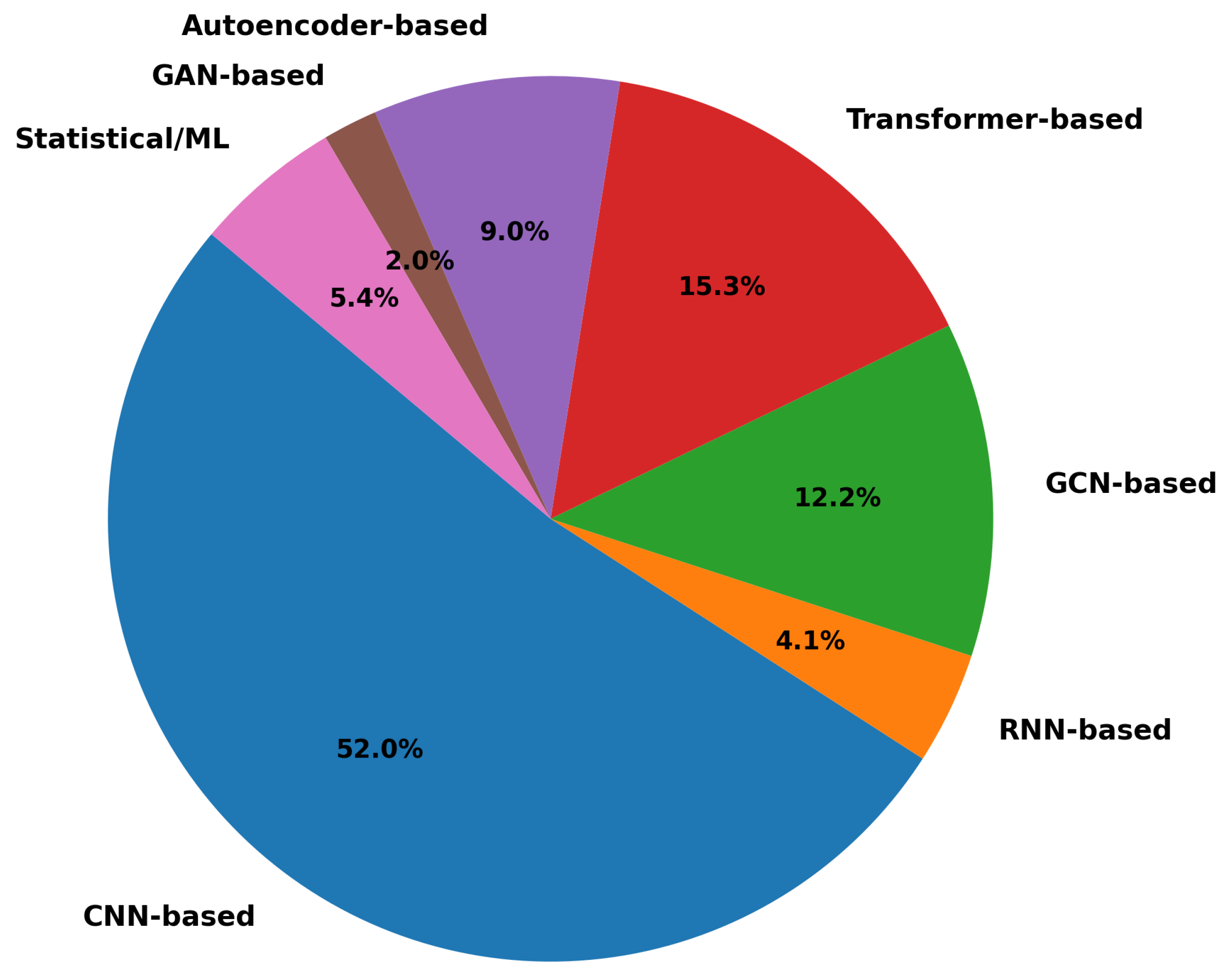
While the number of publications has increased, the methodological landscape has also diversified, as shown in Figure 2. Based on the final screened set of studies, a quantitative breakdown of architectural categories shows that Convolutional Neural Network (CNN)-based methods dominate the field (52%), reflecting their strong ability to model local spectral–spatial patterns. Transformers (15%) and graph-based methods (12%) have emerged as important alternatives, offering improved modeling of long-range dependencies and adaptive spatial relationships. Autoencoders (9%) remain relevant, particularly in unsupervised and reconstruction-driven settings, while Recurrent Neural Networks (RNNs) (4%) appear mainly in earlier studies involving temporal modeling. Generative Adversarial Network (GAN)-based methods (2%) have been explored more selectively, often for adversarial learning or feature enhancement. A smaller fraction of studies (5%) still relies on statistical or shallow machine learning approaches, either as baselines or in combination with deep learning frameworks.

To our knowledge, no previous review has focused exclusively on hyperspectral imagery within the context of deep learning-based change detection while also organizing the literature in a structured way across both supervision strategies and architectural families. This paper not only categorizes existing approaches into supervised, unsupervised, and semi-supervised frameworks, but it also organizes them model-wise into CNNs, RNNs, transformers, graph-based networks, autoencoders, GANs, and hybrid architectures. By consolidating these perspectives on a single platform, this review provides a comprehensive reference point for researchers entering or working in the field. Beyond classification and categorization, the review also highlights key trends, recurring challenges, and persistent research gaps identified in the literature, thereby helping to guide future research directions in deep learning-based HSI-CD.

3. Hyperspectral Images Change Detection: Background, Trends, and Challenges

3.1. Hyperspectral Imaging

Hyperspectral imaging is a sophisticated process that achieves high-resolution images by dividing light into many narrow contiguous spectral bands across the electromagnetic spectrum, typically between visible and infrared wavelengths [9]. This technique employs imaging spectrometers and integrates the following two core technologies: remote imaging and spectroscopy. Spectroscopy involves studying light emission or reflection from various materials and examining variations in energy with wavelength. Remote imaging, on the other hand, aims to capture and record the light reflected from terrestrial landscapes. These capabilities allow hyperspectral sensors to detect unique spectral fingerprints, which are characteristic responses of different surface features to specific wavelengths of light, enabling detailed analysis and identification.

The creation of HSIs can utilize a range of electromagnetic measurements, with common techniques including Raman spectroscopy, middle-infrared (MIR), near-infrared (NIR), and visible (VIS) spectra. Emerging technologies, such as confocal laser microscopy scanners, are also enhancing the scope of hyperspectral imaging. These scanners measure the entire emission spectrum for each pixel at specific excitation wavelengths, significantly improving the spectral resolution. This resolution increases with the number of spectral channels captured within a defined wavelength range, providing a sharper and more precise representation of the observed area. Thus, hyperspectral imaging has revolutionized our understanding of Earth, other planets, and the broader space domain, with applications spread across medicine, biogeochemistry, biophysics, industrial monitoring, and remote sensing, offering profound insights and practical utility in various fields [10,11].

To give a clearer picture of how these ideas translate into practice,

Table 1. Summary of hyperspectral Earth observation satellites.

Satellite	Status	Launch	Total Bands (Range)	Spatial Res.
EO-1 Hyperion [12]	Retired	2000	220 (0.4–2.5 $\mathsf{\mu }$m)	30 m
Proba-1 CHRIS [13]	Retired	2001	63 (0.4–1.05 $\mathsf{\mu }$m); 18 bands at 17 m	17–36 m
HJ-1A HSI [14]	Retired	2008	115 (0.45–0.95 $\mathsf{\mu }$m)	100 m
IMS-1 HySI [15]	Retired	2008	64 (0.4–0.95 $\mathsf{\mu }$m)	505 m
HICO (ISS) [16]	Retired	2009	128 (0.35–1.08 $\mathsf{\mu }$m)	90 m
Gaofen-5 AHSI [17]	Active	2018	330 (0.4–2.5 $\mathsf{\mu }$m)	30 m
PRISMA [18]	Active	2019	240 (0.4–2.5 $\mathsf{\mu }$m)	30 m
EnMAP [19]	Active	2022	224 (0.42–2.45 $\mathsf{\mu }$m)	30 m
ZY-1 02D [20]	Active	2019	166 (0.4–2.5 $\mathsf{\mu }$m)	30 m
Gaofen-5 02 [21]	Active	2021	330 (0.4–2.5 $\mathsf{\mu }$m)	30 m
HySIS [22]	Active	2018	256 (0.9–2.5 $\mathsf{\mu }$m)	30 m
HISUI (ISS) [23]	Active	2019	185 (0.4–2.5 $\mathsf{\mu }$m)	$20\times 31$ m
DESIS [24]	Active	2018	235 (0.4–1.0 $\mathsf{\mu }$m)	30 m
EMIT [25]	Active	2022	285 (0.38–2.5 $\mathsf{\mu }$m)	60 m
OSK GHOSt [26]	Active	2023	512 (0.4–2.5 $\mathsf{\mu }$m)	8 m
Zhuhai-1 OHS [27]	Active	2018	32 (0.4–1.0 $\mathsf{\mu }$m)	10 m
Carbon Mapper [28]	Active	2024	400+ (VIS-SWIR, 0.4–2.5 $\mathsf{\mu }$m)	30 m

lists the main hyperspectral satellites that have been launched so far, both active and retired. The table shows when each mission was launched, how many spectral bands it captured, the wavelength range, and the level of spatial detail. Early missions like EO-1 Hyperion and Proba-1 CHRIS were essentially pathfinders, proving that spaceborne hyperspectral imaging was possible. Since then, systems such as PRISMA, EnMAP, and Gaofen-5 have steadily improved image quality and coverage, while newer constellations from Orbital Sidekick and Carbon Mapper move toward a future of more frequent, commercial-grade monitoring. Together, these satellites trace the story of hyperspectral Earth observation, moving from experimental demonstrations to today’s operational and commercial systems and showing how far the technology has come in just a couple of decades.

3.2. Hyperspectral Change Detection: From Traditional Machine Learning to Deep Learning Models

Any classification problem can be mathematically formulated as an optimization task, where a mapping function $f(·;\theta )$ with or without learnable parameters $\theta$ receives an input data sample and transforms it into a corresponding label category c. The function $f:X\to Y$ is designed to minimize the discrepancy between the predicted output and the ground truth label.

In the context of HSI classification and change detection, the objective is to categorize each pixel $x_i\in {\mathbb{R}}^{\mathrm{nbands}}$ in the HSI scene $X\in {\mathbb{R}}^{n_1\times n_2\times \mathrm{nbands}}$ into one of the predefined mutually exclusive land cover classes. The result is a classification map

$$Y\in {\{1,\dots ,n_{\mathrm{classes}}\}}^{n_1\times n_2}.$$

(1)

To facilitate learning and optimization, it is common to binarize each class label using one-hot encoding, such that

$$Y\in {\{0,1\}}^{n_1\times n_2\times n_{\mathrm{classes}}}.$$

(2)

The mapping function $f(X;\theta )=Y$ then assigns a one-hot vector label $y_i\in {\mathbb{R}}^{n_{\mathrm{classes}}}$ to each spectral pixel $x_i$.

In hyperspectral change detection (HSI-CD), the task is to identify changes across temporally separated observations of the same geographical region. Let $X^{\left(t_1\right)},X^{\left(t_2\right)}\in {\mathbb{R}}^{n_1\times n_2\times \mathrm{nbands}}$ be two HSIs acquired at times $t_1$ and $t_2$, respectively. The change detection function

$$f_{\mathrm{cd}}:(X^{\left(t_1\right)},X^{\left(t_2\right)})\to C$$

(3)

maps the pair of temporal observations to a binary or multi-class change map

$$C\in {\{0,1,\dots ,n_{\mathrm{changes}}\}}^{n_1\times n_2}$$

(4)

indicating the presence or type of change at each spatial location. The goal is to learn $f_{\mathrm{cd}}$ such that it minimizes the discrepancy between the predicted change map and the reference change annotations, while effectively capturing spectral, spatial, and temporal variations in the data.

The body of literature contains a significant number of studies on HSI-CD. These methods are often derived from algorithms and techniques found in computer vision and pattern recognition, showcasing a diverse range of approaches and learning techniques. In this regard, several taxonomies have been proposed to categorize existing change detection methods, reflecting the diversity in data modalities, supervision strategies, feature extraction techniques, and decision models. As a result, they can be categorized into multiple groups based on several factors, ranging from unsupervised methods, such as change vector analysis (CVA) [29], principal component analysis (PCA) [30], multivariate alteration detection (MAD) [31], EM-based thresholding of difference images using mixture models [32], generalized Gaussian modeling [33], k-means clustering [34], Hopfield neural networks for context-sensitive label relaxation [35], and kernel-based techniques that project features into higher-dimensional spaces for improved separability [36,37], to supervised methods such as post-classification comparison, where independently classified maps are differenced to detect changes [38], support vector machines (SVMs) [39], and radial basis function (RBF) neural networks trained to model nonlinear temporal transitions [40]. These techniques span a variety of strategies, from statistical classifiers to deterministic models, and from spectral-based methodologies to spatial or spectral–spatial approaches.

In HSI-CD, the goal is to learn a mapping function $f_c:X\to Y$, where X represents multitemporal hyperspectral observations and Y denotes the binary or multi-class change map. In DL-based models, this global mapping is decomposed into a sequence of hierarchically structured sub-functions, such that the following holds:

$$Y=f_c\left(X\right)=f^{\left(L\right)}\left(f^{(L-1)}(\cdots f^{\left(1\right)}\left(X\right))\right)$$

(5)

where L is the number of layers in the network. Each intermediate layer $f^{\left(l\right)}$ transforms the input using a parametric function of the following form:

$$X^{\left(l\right)}=f^{\left(l\right)}(X^{(l-1)};W^{\left(l\right)},b^{\left(l\right)})=\sigma (W^{\left(l\right)}{X}^{(l-1)}+b^{\left(l\right)})$$

(6)

where $W^{\left(l\right)}$ and $b^{\left(l\right)}$ denote the weight matrix and bias vector of layer l, respectively, and $\sigma (·)$ is a non-linear activation function. This layer-wise representation follows the “divide-and-conquer” principle, where complex mappings are approximated through the composition of simpler transformations.

Despite the effectiveness of hierarchical function composition in DL-based HSI-CD models, designing architectures that can fully exploit the intricate characteristics of hyperspectral data remains a non-trivial task. HSIs possess hundreds of contiguous spectral bands, and changes can manifest in subtle spectral shifts, spatial patterns, or temporal dynamics. HSIs comprise hundreds of bands, leading to enormous spectral dimensionality with high redundancy and strong spatial correlation between neighboring pixels [41]. This “data overload” together with multitemporal inconsistencies (e.g., seasonal changes, illumination differences, and sensor noise) injects significant variability unrelated to true change signals [42]. Moreover, the change detection setting suffers from acute class imbalance (vastly more no-change pixels than changed ones) and a scarcity of labeled samples (since obtaining ground-truth change maps is costly and laborious) [43]. Compounding these challenges, models trained on one scene or sensor often face domain shift when applied to another due to differences in spectral signatures and acquisition conditions [44]. These factors motivated the development of specialized deep learning architectures to robustly extract discriminative spectral–spatial–temporal features and generalize across domains. For instance, convolutional neural networks (CNNs), especially 3D CNNs or dual-stream CNNs, are employed to capture local spectral–spatial context, effectively modeling inter-band relationships and spatial neighborhoods [45]. Recurrent neural networks (RNNs), such as long short-term memory (LSTM) units, have been integrated to handle sequential multi-date information and align temporal dynamics, thereby addressing temporal inconsistency [46]. Transformers with spectrum-aware attention mechanisms further enable learning of long-range dependencies and cross-band feature interactions beyond the reach of localized CNN kernels [47,48]. Graph neural networks (GNNs) have also gained attention, utilizing graph-based representations of HSI pixels or areas to disseminate information and leverage the inherent manifold structure. This method has been demonstrated to be advantageous for learning with a limited number of labels and for understanding spatial relationships [49].

In recent years, the capacity of ANN, particularly in the DL form, to approximate complex functions has garnered significant attention in remote sensing and hyperspectral analysis. DL models have rapidly become indispensable in the HSI-CD domain. The modular design of modern DL architectures, comprising convolutional, recurrent, attention-based, or graph-theoretic components, has enabled researchers to explore increasingly sophisticated solutions tailored to specific HSI-CD challenges. Building on this foundation, we now highlight key architectural and methodological patterns that have emerged in DL-based HSI-CD research since 2018.

3.3. Key Obsevations of Trends and Challenges in DL for HSI-CD

• Early deep learning research in HSI-CD was dominated by CNN-based architectures, particularly Siamese frameworks designed to extract and compare spectral–spatial features from bi-temporal hyperspectral images [50]. Both 2D and 3D CNN variants were widely adopted, with 3D CNNs offering stronger modeling of spectral–spatial correlations and 2D CNNs providing simpler and more computationally practical alternatives when applied to stacked bands or reduced representations. Many of these models were further enhanced with attention mechanisms to emphasize informative spectral bands and spatial regions; for example, SSA-SiamNet incorporated spectral–spatial attention within a Siamese CNN framework [50]. In parallel, encoder–decoder architectures inspired by U-Net were adapted to formulate HSI-CD as a pixel-level segmentation problem. Overall, these developments established CNN-based Siamese and encoder–decoder models as the foundational deep learning paradigm in early HSI-CD research.
• Inspired by advances in computer vision, researchers have introduced transformer architectures and attention modules into HSI change detection [41,51,52]. Recent models employ spectral and spatial self-attention to capture long-range dependencies across hundreds of bands and broad areas. For example, a Spectral–Spatial–Temporal Transformer (SST-Former) was proposed to jointly model pixel embeddings across the spectral domain, spatial neighborhoods, and the two time points [41]. Such transformer-based HSI-CD models achieved accuracy gains by better modeling subtle, global changes. However, purely transformer networks tend to be very complex and prone to overfitting given limited HSI training samples. To mitigate this, hybrid designs are common for example combining CNN backbones for local feature extraction with transformer or attention layers on top for global context. Lightweight attention modules and gating mechanisms have been used to reduce model complexity while still leveraging attention HyGSTAN uses spectral similarity filtering to reduce redundant bands, plus gated spectral–spatial and spectral–temporal attention blocks to focus on meaningful changes [41].
• Although early deep learning methods for HSI-CD were predominantly developed in supervised settings, recent research has shown a clear shift toward semi-supervised, unsupervised, and self-supervised learning frameworks that reduce dependence on dense ground-truth annotations. This transition reflects a broader effort in the literature to make HSI-CD models more label-efficient while still preserving discriminative spectral–spatial representations. Among these directions, self-supervised learning has emerged as a particularly active area. For example, HyperNet introduced a pixel-level self-supervised framework that aligns features from the same spatial location across two temporal acquisitions, encouraging the learning of change-invariant representations without explicit labels [53]. Similarly, HyperSST adopts a hypergraph-based self-supervised strategy that combines contrastive learning with a generative pretext task to capture spectral–spatial–temporal relationships from unlabeled multitemporal HSIs [54]. In parallel, semi-supervised methods have also gained attention by using a limited set of labeled pixels together with unlabeled data through mechanisms such as consistency regularization and graph-based propagation. For instance, one recent approach integrates a GNN with a convex deep model to spread limited supervisory information across graph-structured representations for label-efficient HSI-CD [55]. Together, these developments indicate a strong methodological trend toward label-efficient learning paradigms in HSI-CD.

The HSI-CD field has undergone a clear evolution throughout its progression. Early works built on traditional change detection (change vector analysis and image differencing) by introducing deep feature extractors and achieved better results largely due to more expressive representations. As architectures grew more sophisticated, the accuracy on benchmark datasets steadily improved. A 2019 IEEE review already foresaw deep learning becoming central to HSI-CD [56], and a meta-analysis in 2022 confirmed that deep models outperformed classical methods by a wide margin in CD tasks [57]. Since then, breakthroughs include the use of transformers in HSI-CD, which significantly enhanced the modeling of spectral–spatial interactions, the rise of self-supervised HSI-CD, enabling models to pretrain on unlabeled data and thereby improve performance with limited labels [58]. The trajectory from simple CNN baselines to sophisticated transformers, GNNs, and theory-driven networks shows an overall pattern of increasing model complexity and capability, paired with a recent emphasis on data efficiency and generalization. The major surveys in the literature concur that emerging directions revolve around making HSI-CD methods more accurate, more data-efficient, and more adaptable to real-world conditions. Despite these advances, challenges persist. Based on a focused analysis of published papers, the key challenges in HSI-CD using DL are outlined below:

• HSIs contain hundreds of spectral bands, many of which are highly correlated or noisy. This high dimensionality increases feature redundancy, computational burden, and the risk of overfitting, especially when training data are limited.
• Annotated HSI-CD datasets are scarce because producing reliable pixel-level change labels is expensive and labor-intensive. In addition, the strong imbalance between change and no-change classes further complicates model training and evaluation.
• Variations in illumination, seasonal conditions, atmospheric effects, and sensor characteristics can introduce spectral differences that are unrelated to actual land-cover change, making it difficult to isolate true change patterns.
• Deep models trained on a particular scene or sensor often show reduced performance when transferred to other datasets or acquisition conditions due to domain shift and spectral heterogeneity.
• Many DL-based HSI-CD models remain difficult to interpret, making it challenging to determine which spectral–spatial–temporal cues are driving the final prediction.
• Deep architectures such as 3D-CNNs and transformer-based models often require substantial memory and computational resources, which can limit their practicality in large-scale, real-time, or onboard deployment settings.

Despite the aforementioned challenges, researchers continue to make notable progress in HSI-CD by thoughtfully selecting and tailoring deep learning models to the unique characteristics of HSI data. The careful choice of architectures, learning paradigms, and enhancement strategies ranging from spectral attention to multi-scale feature fusion allows for improved accuracy and adaptability without significantly compromising computational efficiency. As a result, a rich and diverse ecosystem of deep learning frameworks has emerged, each designed to tackle specific dimensions of the HSI-CD problem. The following section provides an in-depth look at this evolving architectural landscape, tracing the trajectory from convolutional and recurrent models to the latest advancements in transformer-based, generative, and graph-driven approaches.

4. Architectural Landscape of DL Approaches

4.1. CNN-Based Methods

The CNN, quite possibly the most broadly utilized DL model, was initially intended to handle information from images. On account of this characteristic, it is appropriate for preparing multi-band remote sensing image data in which pixels are arranged consistently.

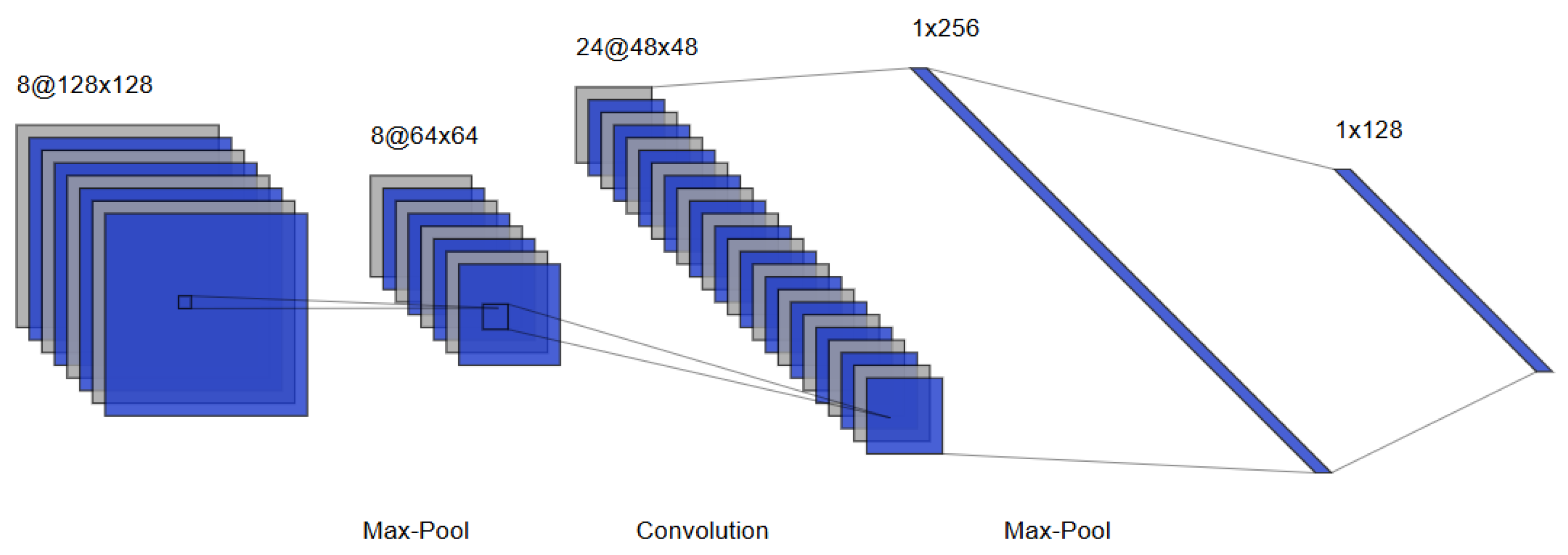
CNN has become a cornerstone in hyperspectral change detection (HSI-CD) because of its strength in learning both spatial and spectral features from high-dimensional image data. A typical CNN is built from three main components: convolutional layers, pooling layers, and fully connected (dense) layers, as illustrated in Figure 3.

In the convolutional layer, small trainable kernels (or filters) slide across the input and generate feature maps that capture local structures such as edges, textures, or spectral patterns. This operation allows the network to automatically learn useful representations directly from the data rather than relying on handcrafted features. Mathematically, for an input $X\in {\mathbb{R}}^{H\times W\times C}$ and a kernel $K\in {\mathbb{R}}^{k_h\times k_w\times C}$, the convolution is expressed as follows:

$$Y_{i,j}={\displaystyle \sum _{m=1}^{k_h}}{\displaystyle \sum _{n=1}^{k_w}}{\displaystyle \sum _{c=1}^C}{K}_{m,n,c}·X_{i+m,j+n,c},$$

(7)

where $(i,j)$ is the position in the output feature map Y. In practice, this means the kernel K scans across the input X and combines local information into new features. By repeating this process over the entire image, the network learns filters that respond to patterns regardless of their position, making the features translation-invariant—an ability that is particularly important for detecting subtle changes between multitemporal images.

Next, pooling layers reduce the size of the feature maps. This step not only speeds up computation but also makes the learned features more robust to small shifts or noise. Common pooling strategies include max pooling, average pooling, and sum pooling [60]. For example, max pooling is expressed as follows:

$$Y_{i,j}=\underset{(m,n)\in \mathcal{R}}{max}{X}_{i+m,j+n},$$

(8)

where $\mathcal{R}$ is the pooling region. Intuitively, this means that instead of keeping every detail, the network retains only the most important signals from each region.

Finally, fully connected (dense) layers pull together all the extracted features and feed them into a classifier. A typical transformation is

$$\widehat{y}=\sigma (Wx+b),$$

(9)

where x is the flattened feature vector, W and b are learnable weights and biases, and $\sigma (·)$ is an activation function such as softmax or sigmoid. This step turns the hierarchical features learned by the CNN into predictions about whether a pixel belongs to a change or no-change class.

Overall, CNNs stand out because they can naturally capture both spectral and spatial information in a hierarchical way. This makes them well-suited to identifying subtle differences across time while preserving the broader context of the scene. Many architectures have built on this foundation. For example, GETNET [61] and TDSSC [62] exploit 2D/3D convolutions to model spectral–spatial features, while Robust PCANet [63] integrates PCA-filtered inputs to boost generalization under noise. More recent designs push CNNs further: the 3D-Wavelet Active CNN [64] uses wavelet decomposition and active learning for denoising and feature extraction; SFBS-FFGNet [65] employs a dual-branch strategy with slow–fast band selection and feature fusion; and RSCNet [66] introduces residual self-calibrated convolutions to adapt receptive fields and reduce irrelevant information.

In addition to standard CNN backbones, more advanced designs have emerged that incorporate pyramid structures and recurrent units. For instance, the Multiscale Pyramid Network with Spatial-Spectral Residual Attention [67] uses deep convolutional pyramids combined with cross-domain attention to better capture spatial-spectral relationships. ML-EDAN [68] extends the encoder–decoder framework with contextual attention modules and inserts LSTM units at the bottleneck, allowing the model to capture temporal dynamics across multitemporal hyperspectral inputs. Similarly, the Multipath ConvLSTM CNN architecture [69] integrates recurrent ConvLSTM units with CNN-based multiscale feature extraction, boosting sensitivity to complex and subtle scene changes. Beyond these hand-crafted designs, the Self-Perception Network with Evolutionary Search (SPNA-CA) [70] explores automated neural architecture search, tailoring optimal CNN architectures for HSI-CD and even enabling knowledge transfer across datasets. Together, these strategies show how CNN-based methods are continuously evolving, blending pyramid designs, recurrent modeling, residual learning, and attention mechanisms to cope with the high dimensionality and spectral variability that make hyperspectral change detection so challenging.

Moreover, several recent works continue to innovate within the CNN framework by leveraging multipath structures, band engineering, and self-supervised learning. Although autoencoders represent a distinct category of deep learning models, M3CAN [71] adopts a 3D convolutional autoencoder entirely built from convolutional layers. This design aligns it with CNN-based methods, enabling the extraction of hierarchical spatial–spectral features from hyperspectral volumes while reducing redundancy in an unsupervised manner. Similarly, the framework proposed by Zhang et al. [72] combines a CNN-based encoder–decoder structure with contrastive self-supervised learning, where the CNN encoder learns discriminative spatial-spectral embeddings and the decoder reconstructs inputs in a self-supervised phase before fine-tuning for change detection. MTC-Net [58] introduces a Siamese architecture with 3D spatial–spectral attention modules to tackle anomalous change detection, aligning multitemporal features via contrastive learning. MMSRC [73] employs multidirectional and multiscale residual CNN blocks enhanced with spectral–spatial attention to capture intricate inter-band relationships and directional textures. In a different direction, the work by Shammi and Du [74] augments CNN-based supervised change detection with explicit nonlinear band expansion techniques, enriching the spectral diversity for better separability. These methods demonstrate the adaptability of CNNs to diverse HSI-CD challenges, including anomalous change detection, spectral redundancy, and multi-class differentiation, all while maintaining computational efficiency and scalability.

Several recent CNN-based architectures have been proposed to address challenges such as spatial resolution mismatch, inter-temporal alignment, and hybrid feature learning. SPCNet [75] integrates subpixel convolution layers into a residual CNN backbone to align hyperspectral images of varying spatial resolutions, enabling robust subpixel feature learning. Similarly, the subpixel convolutional residual network proposed in [76] fuses multiscale CNN features with resolution-adaptive convolution blocks for precise spatial–spectral representation. SSA-SiamNet [77] utilizes a Siamese CNN architecture augmented with spectral–spatial-wise attention to enhance inter-temporal feature discrimination. In a complementary direction, the method in [78] fuses handcrafted spectral–temporal features with deep CNN-derived representations, showcasing the potential of hybrid feature integration for boosting generalization. These methods reflect the versatility of CNN-based frameworks, especially when augmented with attention, multiscale processing, and domain knowledge.

4.2. RNN-Based Methods

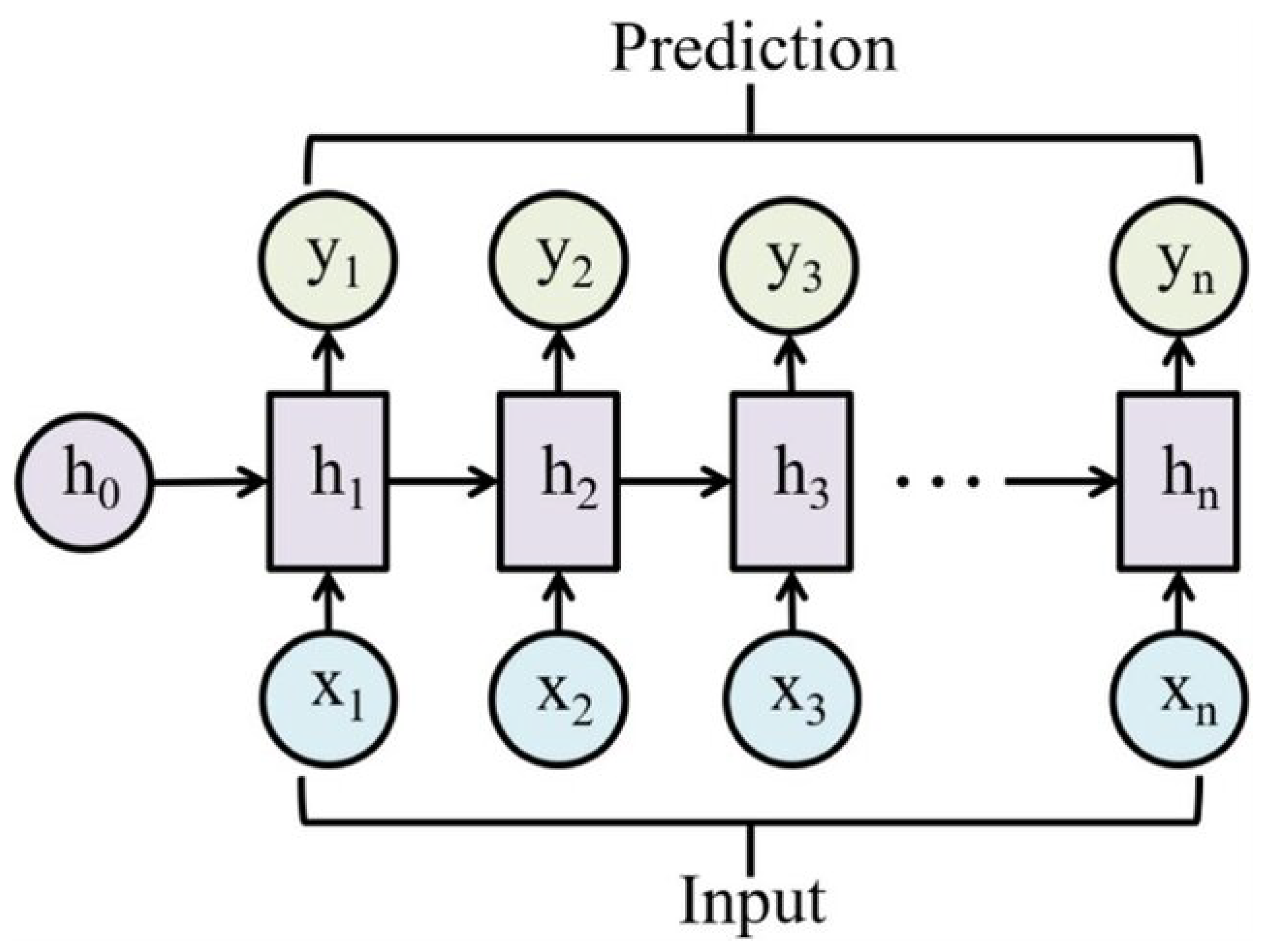
Recurrent neural networks (RNNs), illustrated in Figure 4, play an important role in HSI-CD by capturing the temporal or sequential dependencies present in multitemporal data. Unlike feed-forward models that process inputs independently, RNNs maintain a hidden state that updates as new inputs arrive. This mechanism allows the network to “remember” past observations and use them to interpret current ones. Because of this ability to model sequences, RNNs are widely applied in domains that depend on temporal context, such as natural language processing (NLP) [79], image captioning, speech recognition, etc. In the context of hyperspectral change detection, this same strength enables RNNs to track subtle spectral–spatial changes over time and make more informed predictions.

RNNs are designed to model sequential data by maintaining a hidden state that evolves over time. In HSI-CD, where the temporal dimension plays a critical role, RNNs can effectively capture spectral–temporal dependencies between multitemporal observations. This sequential modeling is crucial for detecting subtle or progressive changes that might be overlooked by static methods.

Formally, for an input spectral feature $x_t$ at time t, a vanilla RNN computes the hidden state $h_t$ [81] as follows:

$$h_t=\sigma (W_x{x}_t+W_h{h}_{t-1}+b)$$

(10)

where $\sigma (·)$ is a non-linear activation function (e.g., tanh or ReLU); $W_x$ and $W_h$ are learnable weight matrices for the input and hidden state, respectively; and $\mathbf{b}$ is the bias vector.

The final decision (change or no change) is often made based on the last hidden state or a function of the sequence of hidden states:

$$\widehat{y}=f_{\mathrm{out}}\left({\mathbf{h}}_T\right)$$

(11)

where T is the number of timesteps and $f_{\mathrm{out}}$ is typically a softmax or sigmoid classifier.

LSTMs [82] extend this formulation with gating mechanisms, input, forget, and output gates, that control the flow of information into a memory cell. The cell state $c_t$ and hidden state $h_t$ are updated as follows:

$$c_t=f_t\odot c_{t-1}+i_t\odot tanh(W_c{x}_t+U_c{h}_{t-1})$$

(12)

$$h_t=o_t\odot tanh\left(c_t\right)$$

(13)

where $i_t$, $f_t$, and $o_t$ are the input, forget, and output gates, respectively (all computed using sigmoid activations); $x_t$ is the input at time t; and ⊙ denotes element-wise multiplication. These gates enable LSTMs to learn what to retain or forget at each step, which is valuable for change detection because the model can ignore irrelevant temporal variations (such as illumination changes) and focus on persistent changes.

RNNs were embraced in HSI-CD starting in the late 2010s as researchers recognized the need to model temporal dynamics beyond simple image differencing. One early landmark was the work of Lyu et al. [83], who trained an RNN to learn a transferable change rule for land cover change detection. This study shows that an RNN could internalize how spectral patterns transition between times and apply that knowledge to detect changes in new scenes. Building on this idea, Song et al. [84] introduced a fully DL framework called Recurrent 3D Fully Convolutional Network (Re3FCN). In Re3FCN, a 3D convolutional neural network first extracts spectral–spatial features from two input HSI cubes (one for each date), and then a ConvLSTM layer (a convolutional LSTM) is used to model the temporal relationship between the feature maps. The ConvLSTM processes the two time feature volumes sequentially: it treats the time-1 feature map as input at $t=1$ and the time-2 feature map at $t=2$, carrying over a hidden state that captures changes. Because ConvLSTM replaces the weight matrices in LSTM with learnable convolution kernels, it can preserve the 2D spatial structure of features while it “recur” over time. Shi et al. [69] proposed MP-ConvLSTM, a multipath convolutional LSTM architecture that integrates spectral–spatial features extracted via Siamese CNNs with multi-scale ConvLSTM branches. These branches capture diverse temporal dynamics at multiple scales, while an Efficient Channel Attention (ECA) module further enhances the fusion of spatial, spectral, and temporal cues, enabling both binary and multi-class change detection. In another study, Ref. [68] work introduces a multilevel encoder–decoder attention network (ML-EDAN) which incorporates an LSTM block within its architecture to model temporal dependencies. The framework consists of parallel CNN-based encoders for bi-temporal HSIs, extracting spatial–spectral features at multiple levels. These features are then fed into a shared LSTM module that captures sequential correlations between the two time steps. Finally, a decoder reconstructs the change map using learned attention weights and fused temporal features. Additionally, one method applies a CNN to extract spectral–spatial features, and these features are then flattened and fed sequentially into a RNN composed of LSTM units [85]. The LSTM learns to accumulate temporal context across the input sequence, allowing it to model progressive and subtle changes in land cover. The final hidden state from the LSTM is then passed through a fully connected layer with a sigmoid activation to predict binary change or no change. In summary, RNN-based methods have carved out a significant place in HSI change detection: they introduce memory and sequence modeling into the problem, enabling the generation of change maps that account for the temporal evolution of spectral signatures.

4.3. Autoencoders

Autoencoders are a class of unsupervised neural networks that were first popularized in the 1980s for dimensionality reduction and feature learning tasks [86]. Their modern resurgence, particularly since the 2000s with the advent of DL, has made them vital tools for tasks such as denoising, anomaly detection, and representation learning [87,88]. At their core, autoencoders aim to learn a compressed latent representation of input data that captures its essential characteristics, enabling accurate reconstruction. This capacity makes them particularly well suited for HSI data, where data are high-dimensional and often redundant. In HSI-CD, autoencoders are used to extract spectral–spatial representations and reduce dimensionality, thereby improving the discriminative power of learned features. Moreover, their unsupervised nature is advantageous in remote sensing scenarios where labeled data are limited or expensive to obtain.

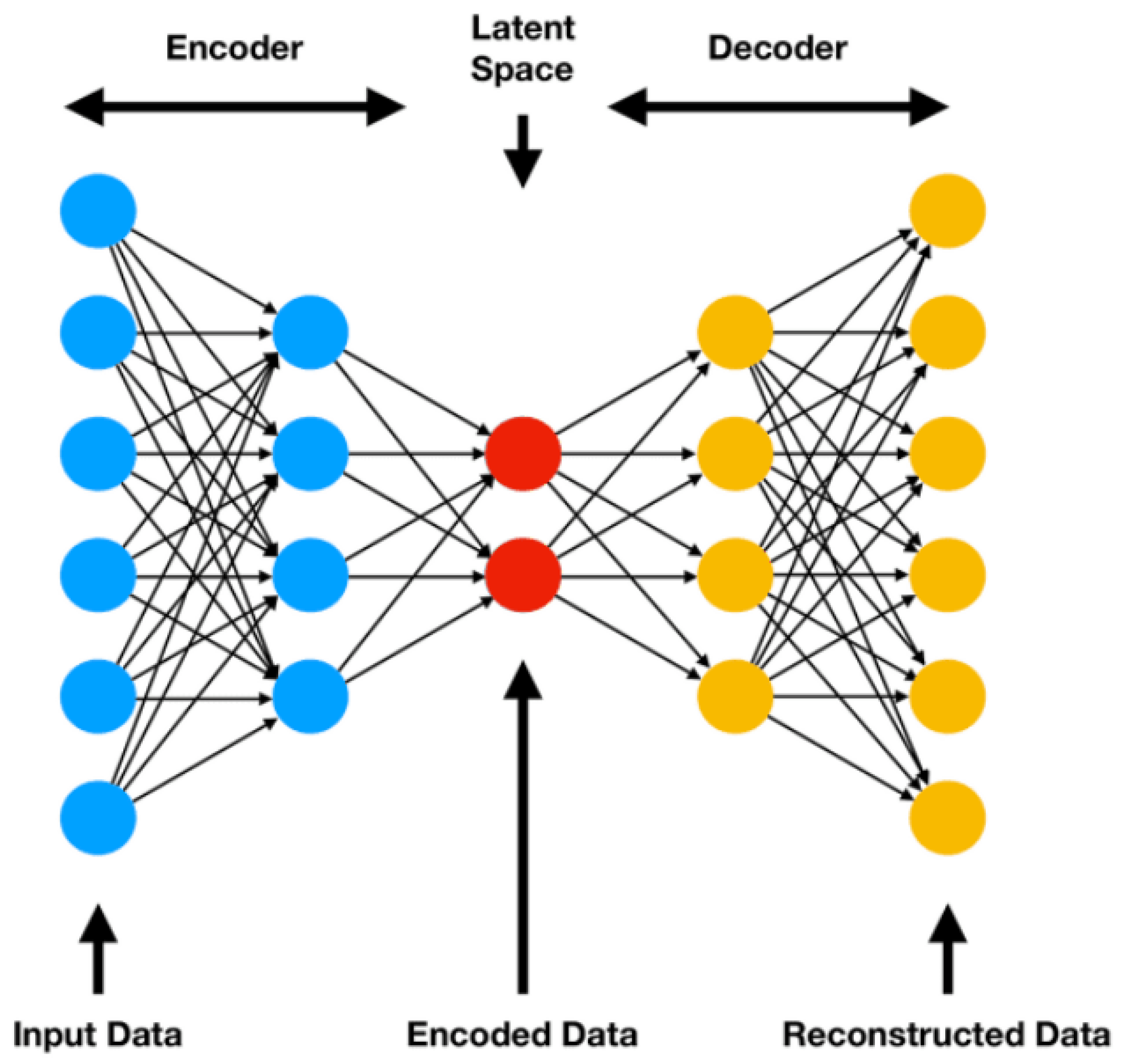
An autoencoder consists of two main components, the encoder and the decoder, as shown in Figure 5. The encoder $f_{\theta }$ maps the input data $X\in {\mathbb{R}}^{H\times W\times C}$ into a lower-dimensional latent representation $Z\in {\mathbb{R}}^d$. The decoder $g_{\varphi }$ reconstructs the input from the latent code, yielding $\widehat{X}=g_{\varphi }\left(f_{\theta }\left(X\right)\right)$. The network is trained to minimize the reconstruction loss.

Autoencoder-inspired models have become increasingly popular in recent advancements in HSI-CD because of their capability to capture detailed representations in both unsupervised and semi-supervised contexts. These models are particularly advantageous in situations with limited or no labeled data, providing efficient alternatives to traditional handcrafted or simple learning techniques. A prominent line of research explores self-supervised and unsupervised autoencoders for representation learning. Ref. [89] proposed a Self-Supervised Tensor Network (SSTN) that combines tensor decomposition with clustering, jointly learning low-rank spectral and spatial representations. Similarly, Ref. [90] introduced the ACDA framework using Siamese autoencoders to model nonlinear background variation between bi-temporal HSI, identifying anomalies through dual-direction reconstruction errors. Ref. [71] extended this idea with M3CAN, a multi-scale 3D convolutional autoencoder network that extracts deep spectral–spatial features in an unsupervised manner and uses a lightweight supervised classifier, striking a balance between robustness and label efficiency. Ref. [72] further advanced self-supervised pretraining with dual autoencoders aligned by contrastive loss, enhancing feature discrimination with minimal labels. Likewise, Ref. [91] proposed a self-supervised framework (SSCL) that, though not explicitly using an autoencoder, adopts a similar unsupervised-to-supervised transition by refining pseudo-labels via feature consistency and confident learning, reinforcing the versatility of autoencoder style strategies.

Beyond classical encoders, physically guided and interpretable autoencoder variants have emerged to handle spectral inconsistencies and mixed pixels. Ref. [92] proposed a Two-Stream Coupled Autoencoder (TSCA) that integrates intrinsic decomposition modeling into an unsupervised HSI change detection framework. The architecture uses two symmetric encoders to extract abundance features and spectral variation factors, which are then decoded into reflectance-like representations. This process effectively separates environmental influences (like illumination) from material intrinsic properties. A shared decoder and cross-reconstruction mechanism enforce feature alignment and consistency, enhancing unsupervised detection performance. The physically interpretable autoencoder structure enables both dimensionality reduction and robust feature learning without requiring ground-truth labels. Similarly, Ref. [93] proposes DLDINet, a hybrid dictionary learning-guided interpretable network that unfolds iterative sparse coding into a two-stream autoencoder-inspired architecture. It combines a Deep Denoising Module and a Coefficient Updating Module mimicking encoder–decoder behavior while promoting interpretability through dictionary priors. These approaches demonstrate how embedding physical or semantic priors into autoencoder structures can significantly improve robustness and explainability. Another noteworthy contribution is the Adaptive Endmembers Learning (AEL) network [94] which embeds an autoencoder-based unmixing module within a deep change detection framework. Unlike traditional unmixing methods that rely on fixed or predefined endmembers, AEL performs adaptive endmember and abundance learning through unsupervised patch reconstruction. This approach not only captures spectral variability between bi-temporal images but also enhances both binary and multi-class change detection accuracy. By jointly optimizing the unmixing and detection branches, the autoencoder serves as a physically grounded module that improves robustness to mixed pixels and spectral inconsistency. Building on this trend of interpretable and semi-supervised frameworks, another paper introduces a semi-supervised multiscale convolutional sparse coding-guided deep interpretable network (MS-CSC-DINet) [68]. Its architecture includes a sparse reconstruction encoder and a feature embedding decoder, closely mimicking encoder–decoder behavior. By integrating multiscale sparse feature guidance and contrastive learning with a small fraction of labels, the model achieves robust performance with interpretable latent representations. This further reflects the expanding role of autoencoder-style designs in bridging the gap between unsupervised learning and label-efficient deep CD.

4.4. GAN Based Methods

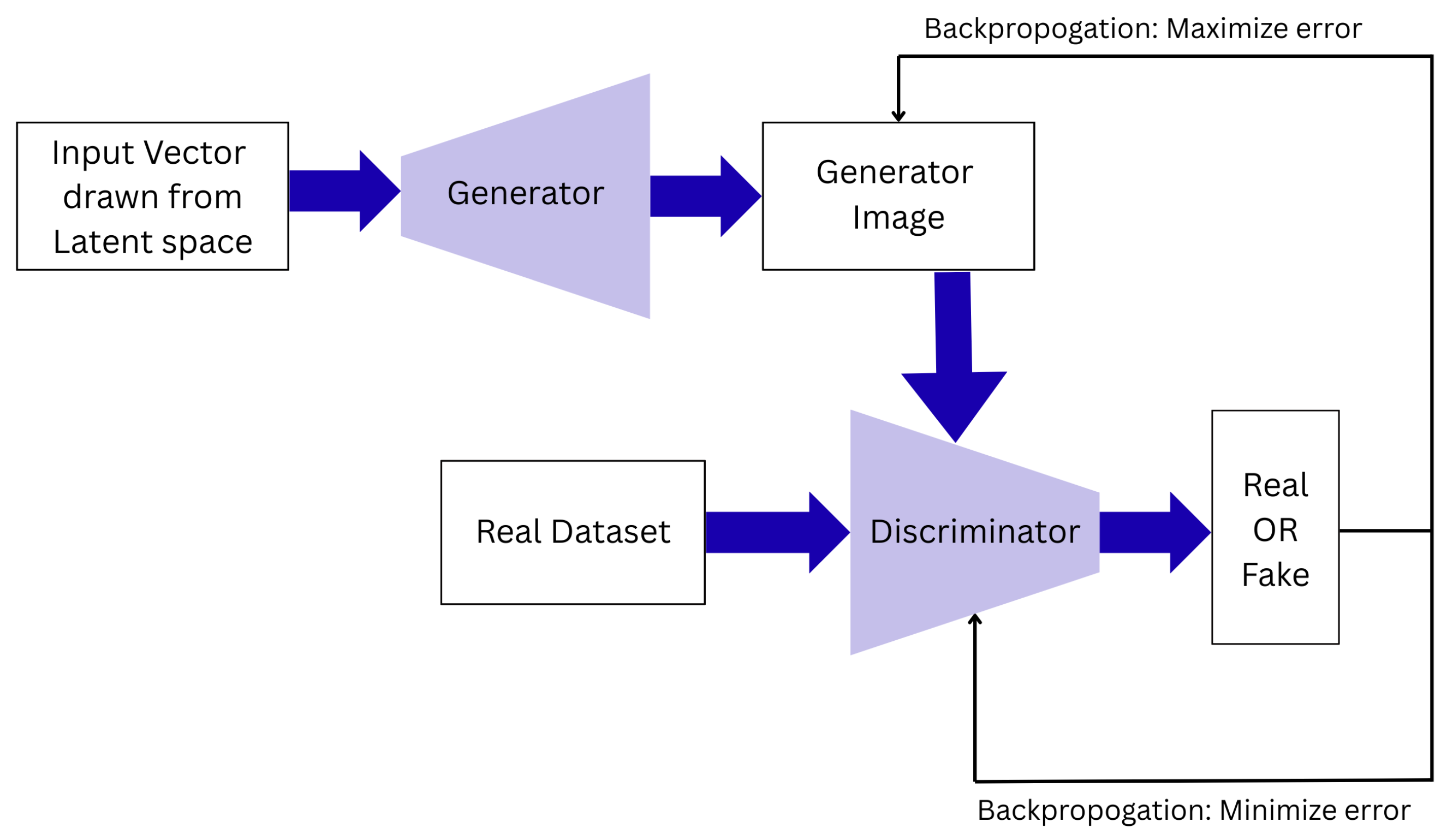
Generative Adversarial Networks (GANs), introduced by Goodfellow et al. (2014) [95], are a class of generative models that learn to synthesize data resembling a target distribution through an adversarial learning process. A GAN comprises two competing neural networks, a generator G and a discriminator D as shown in Figure 6. The generator aims to produce realistic samples from a noise prior $z\sim p_z\left(z\right)$, while the discriminator tries to distinguish between real samples $x\sim p_{\mathrm{data}}\left(x\right)$ and generated samples $G\left(z\right)$. The training objective is formulated as a two-player minimax game:

$$\underset{G}{\min }\underset{D}{\max }{\mathbb{E}}_{x\sim p_{\mathrm{data}}}\left[\log D\left(x\right)\right]+{\mathbb{E}}_{z\sim p_z}\left[\log (1-D\left(G\left(z\right)\right))\right].$$

The equilibrium is reached when the generator’s output becomes indistinguishable from real data, i.e., $D\left(x\right)=0.5$ for all inputs. Variants such as conditional GANs (cGANs) [96], CycleGANs [97], and Wasserstein GANs (WGANs) [98] have further enhanced stability, conditional learning, and domain adaptation capabilities, making GANs applicable across image generation, translation, and representation learning tasks.

In the context of HSI-CD, GANs offer a promising avenue to address critical challenges such as spectral variability, the scarcity of labeled data, and modality mismatch in multitemporal observations. The high spectral dimensionality and limited annotated samples in HSI make unsupervised or semi-supervised learning frameworks highly desirable scenarios in which GANs naturally excel. For instance, an unsupervised spectral mapping framework using adversarial learning was proposed to extract latent spectral representations, followed by spatial refinement for change detection [99]. A hybrid autoencoder GAN model named EFC-AdvNet was introduced to produce binary change maps directly from compressed spectral features, yielding notable gains in detection accuracy [100].

Despite these advances, the application of GANs in HSI-based change detection remains relatively underexplored. Compared to the widespread use of convolutional neural networks, transformers, and autoencoders in this domain, GAN-based frameworks are still in their infancy. This is primarily due to the intrinsic challenges of handling high spectral dimensionality, preserving spectral fidelity in generated samples, and ensuring stable adversarial training. Moreover, there is a lack of standardized benchmarks and comprehensive evaluations, which further impedes progress in this area. As a result, only a limited number of studies have attempted to fully exploit adversarial learning for hyperspectral change detection. Nevertheless, with continued development in generative modeling and hybrid learning strategies, GANs hold considerable potential to advance robust, scalable, and label-efficient solutions for HSI-CD.

4.5. Graph-Based Methods

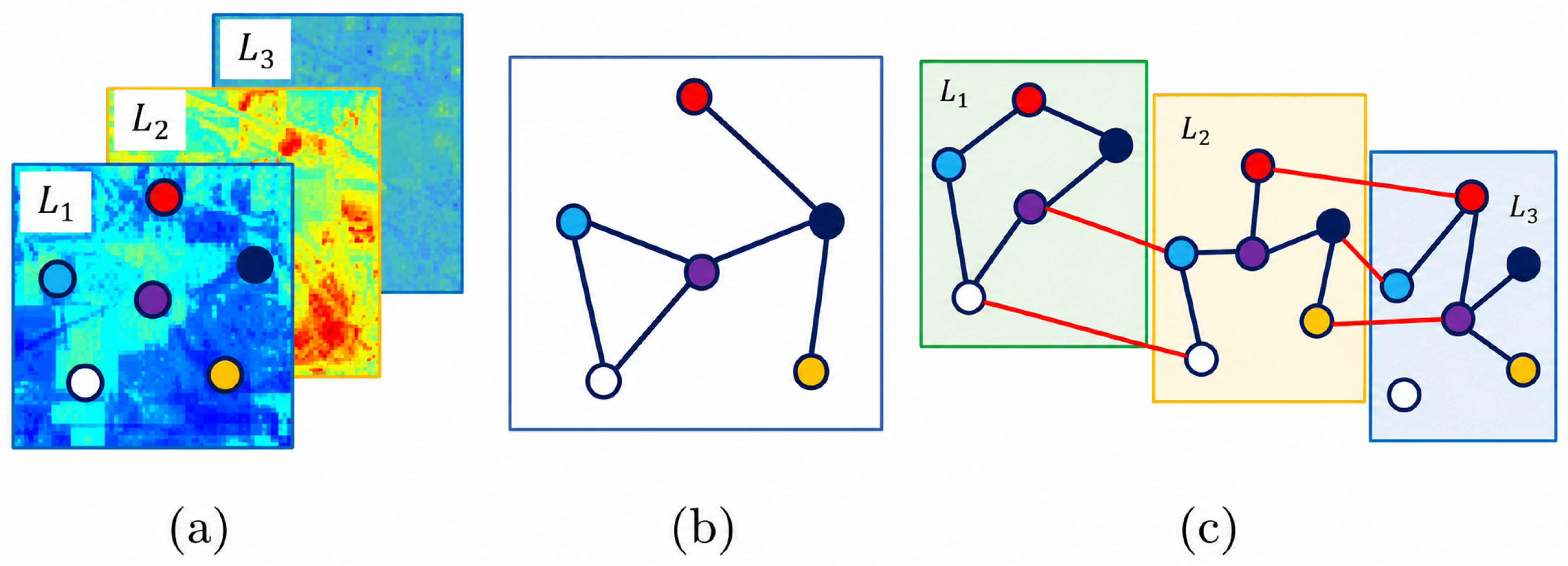
Graph-based methods have emerged as a powerful paradigm for modeling complex spatial-spectral relationships in HSI-CD. At their core, graphs provide a mathematical framework to represent structured data in terms of pairwise relationships. Formally, a graph is defined as $G=(V,E)$, where V is the set of nodes (or vertices) and $E\subseteq V\times V$ is the set of edges connecting pairs of nodes. Each edge $e_{ij}\in E$ may be associated with a weight $w_{ij}$ representing the similarity or affinity between nodes $v_i$ and $v_j$. In the context of HSI, graph nodes can represent pixels, superpixels, or spatial–spectral regions, while edge weights often encode spectral similarity, spatial proximity, or temporal consistency across image acquisitions. The graph structure enables the modeling of both local neighborhoods and nonlocal dependencies, which are especially useful in high-dimensional and spatially structured data like HSI [101]. Figure 7 illustrates how a hyperspectral image can be represented as a graph.

Recent years have seen graph-based models become a prominent paradigm for HSI-CD. GNNs, such as graph convolutional networks (GCNs), gained attention for their ability to handle non-Euclidean data structures, unlike traditional CNNs, which are confined to regular image grids. This flexibility allows GCNs to capture complex topological and contextual relationships (between irregular superpixel regions), which is crucial for modeling the rich spectral–spatial structure of hyperspectral imagery. Early deep learning CD methods based on CNNs achieved success, but often at the cost of losing fine details through downsampling and failing to fully exploit multi-scale spectral information [102]. The first milestone came with the Dual-Branch Difference Amplification GCNs (D2AGCN) [103], which introduced GCNs into HSI-CD. This framework built superpixel graphs to reduce complexity and employed dual GCN branches to amplify spectral difference features across bi-temporal HSIs. Its difference amplification module effectively suppressed redundant background signals while emphasizing meaningful changes, enabling accurate detection under limited labeled data. This was followed by the Complementary Dual-Branch Spatio-Temporal Joint Graph Attention Framework (CSDBF) [104], which extended GCNs with graph attention networks (GATs) and a dual-branch design. By adaptively weighting node relationships through temporal-spatial joint graph attention and fusing a superpixel-level GAT branch with a pixel-level CNN branch, CSDBF captured both global contextual dependencies and fine-grained spectral–spatial details, achieving strong performance even under very low sampling rates.

Addressing the persistent problem of scarce annotations, the Convex Deep Learning Framework (CODE-HCD) [55] integrated a lightweight GNN with a convex Q-quadratic regularizer. This hybrid approach produced a rough solution with GNNs, then refined it through convex optimization to convergence and robustness under extremely low sampling rates. The idea was further refined in the Small-Data Learning Framework with Area-Control (SDL-HCD) [105], which added an explicit area-control mechanism to constrain the detected change regions. This design avoided over- or under-estimation of change extent while maintaining high efficiency, enabling accurate detection with as little as 0.1% labeled data.

Beyond small-data learning, researchers also advanced the representational power of graph-based models. The Graph Transformer-Guided Multitemporal Information Framework (GTransCD) [106] introduced graph transformers to enhance long-range dependency modeling. By applying a transformer to superpixel graphs and coupling it with a gated change fusion unit, GTransCD simultaneously captured local and global features while propagating label information in a semi-supervised setting, thus reducing reliance on annotations. In parallel, hybrid CNN–GCN architectures emerged, exemplified by the Hyperspectral Multilevel GCN and CNN Feature Fusion (HMGCF) model [49]. HMGCF combined a superpixel-level GCN branch with a pixel-level CNN branch, bridged through a graph encoder–decoder that allowed information exchange between graph and grid domains. This design ensured complementary learning, preserving subtle local variations and global contextual consistency in an end-to-end framework.

Most recently, a new frontier was opened with the Quantum Information-Empowered Graph Neural Network (QUEEN-$\mathcal{G}$) [107] fused quantum feature learning with graph-based learning. At the pixel level, a quantum feature module generated unitary quantum representations, while at the superpixel level, a GNN branch captured structural spectral–spatial dependencies. These were fused in a dual-branch framework and classified using a quantum-enhanced classifier, enabling richer feature representations beyond classical models. QUEEN-$\mathcal{G}$ achieved state-of-the-art results across multiple datasets and showed robustness under label scarcity, marking the first integration of quantum information processing into graph-based HSI-CD.

Altogether, these studies trace a clear path in how graph-based methods for HSI-CD have evolved. Step by step, each advancement has broadened the ability of graph-based models to deal with limited labels, irregular structures, and complex dependencies, establishing them as one of the most promising directions for the future of hyperspectral change detection.

4.6. Transformer Based Methods

The goal of transfer learning is to apply the knowledge acquired from different but related tasks to new domains and tasks. The Transformer, first introduced by Vaswani et al. [108] marked a major shift in how we approach sequence modeling. Unlike earlier architectures that relied heavily on RNNs or CNNs, the Transformer is built entirely on attention mechanisms. At its core is the self-attention operation, which allows the model to compare every element in a sequence with every other element, assigning weights that determine how much influence one element should have on another. This design makes it possible to capture long-range relationships in data more effectively than recurrent models, while also allowing computations to run in parallel. The result is a model that is not only faster to train but also highly capable at tasks like machine translation and, more broadly, at any problem that involves processing sequential information. Building on this foundation, Dosovitskiy et al. presented the Vision Transformer (ViT), which demonstrated that a pure Transformer architecture could be successfully adapted to computer vision without convolutional priors [109]. In ViT, images are partitioned into non-overlapping patches that serve as tokens, analogous to words in natural language processing. These patches are linearly embedded and processed through standard Transformer layers, enabling the model to capture global spatial dependencies. When pretrained on large-scale datasets and fine-tuned on downstream benchmarks, ViT achieved competitive or superior performance.

Within this broader transfer-learning paradigm, CDFormer [110] represents a pioneering effort to introduce transformer encoders into HSI-CD. The model views pairs of hyperspectral image patches taken at different times as sequences, adding positional and temporal information so the model knows where and when each pixel comes from. Using multi-head self-attention, it can look across the entire scene and learn how spectral, spatial, and temporal patterns interact. This design allows it to detect changes with very few labeled samples. Song et al. introduced CSANet (Cross-Temporal Interaction Symmetric Attention Network) which extended this idea with symmetric cross-temporal attention, explicitly modeling the relationships between bi-temporal images in a Siamese framework [111].

The progression of transfer-based models in HSI-CD shows a clear path from basic transformer transfer to increasingly specialized designs. Dong et al. [112] developed AMCAN-HMSchA (Abundance Matrix Correlation Analysis Network with Hierarchical Multihead Self–Cross Hybrid Attention) which introduces abundance representation into transformer-style modeling. Hyperspectral pixels are unmixed into abundance matrices using shared endmembers across time, and a HMSchA mechanism learns correlations between the two abundance maps. This hybrid approach addresses mixed-pixel problems common in HSI and improves subtle change discrimination. Shafique et al. [113] proposed SSViT-HCD (Spatial–Spectral Convolutional Vision Transformer for HSI-CD), which combines convolutional feature extractors with a vision transformer backbone. Convolutional layers and a Convolutional Block Attention Module (CBAM) capture fine-grained spectral–spatial patterns locally, while the ViT encoder models long-range dependencies globally. Wang et al. [114] designed TriTF (Triplet Transformer Framework) with two novel branches. The Parents-Temporal Attention (PTA) branch adopts a ternary $T1\to T3\leftarrow T2$ design where the difference image acts as the “child,” fusing temporal information from both times. The Brother-Spatial Attention (BSA) branch finds the most similar patch (“brother”) within a batch and applies cross-attention to capture longer-range spatial interactions. Zhang et al. [115] proposed STFL (Spectrum-Induced Transformer-Based Feature Learning), designed for multiple change detection (MCD) rather than binary detection. Its spectrum-induced transformer computes attention along spectral dimensions to learn long-range inter-band dependencies, while an attention-based detection module emphasizes the most effective bands for detecting and classifying “from-to” changes.

Building on this shift from binary to multi-class change detection, later works began to explore unsupervised and weakly supervised transformer frameworks to further reduce dependence on labeled data. One representative example is PCPTNet (Parallel Compared-and-Stacked Pyramid Transformer Network) [116], which employs dual-stream pyramid transformers to simultaneously learn difference features and fuse contextual information. The Compared Pyramid Transformer (CPT) stream highlights changes directly, while the Stacked Pyramid Transformer (SPT) preserves complementary spectral–spatial details. A superpixel-level joint decision strategy integrates the outputs, enabling multiscale change representation without the need for labels. In contrast to STFL, which adapts spectral attention for multiple change classes, PCPTNet demonstrates how transformer architectures can be transferred into label-free scenarios, aligning with the broader trend toward annotation-efficient HSI-CD. Following this, Chen et al. [117] proposed STSS-Net (Joint Saliency Temporal–Spatial–Spectral Information Network), which explicitly introduces saliency into transformer-based hyperspectral CD. A Spatial Saliency Information Extraction (SSIE) module is used to suppress noise and emphasize spatially relevant pixels, while a Compact High-Level Spectral Information Tokenizer (CHLSIT) compresses redundant spectral channels into compact tokens. These representations are then processed by transformer encoders and decoders to jointly capture temporal, spectral, and spatial dependencies. Compared to PCPTNet’s unsupervised pyramid design, STSS-Net highlights another direction of transfer-based adaptation, where saliency-driven feature selection ensures that only the most meaningful cues are propagated through the transformer layers. Most recently, Huang et al. [118] developed TWBSIT (Temporal Weight-Sharing and Bandwise Spatial-Interacting Transformer), further consolidating semi-supervised learning with transformer-based architectures. TWBSIT introduces a Weight-Sharing Interacting Temporal Attention (WITA) module to capture shared dependencies across time, and a Bandwise Cross-Spatial Attention (BCSA) module to learn spatial interactions across spectral bands. Its training is guided by Conflict HyperMatch, a semi-supervised strategy that jointly leverages discrepancy and consistency losses to exploit both labeled and unlabeled data.

Overall, the reviewed studies illustrate how transfer learning has become a cornerstone for advancing HSI-CD. By drawing on transformer and attention architectures originally developed for natural language processing and computer vision, researchers have been able to design models that handle the unique challenges of hyperspectral data, outlined as follows: high spectral dimensionality, temporal variability, and limited labeled samples. The diversity of approaches ranging from sequence-based transformers to hybrid CNN-ViT designs, spectral–spatial attention modules, unmixing-driven hybrids, and semi/unsupervised frameworks demonstrates the flexibility of transfer learning as a paradigm. More importantly, these models collectively highlight a shift in the field: away from handcrafted feature engineering and purely supervised pipelines, toward generalizable, data-efficient, and task-adaptive architectures that can operate under real-world constraints.

5. Learning Strategies

In addition to the type of models in DL, DL allows models to also implement different learning strategies. The success of deep learning in HSI-CD also depends heavily on the learning strategies used during model training and adaptation. Since hyperspectral datasets often suffer from limited annotations, high spectral redundancy, and significant distribution shifts across sensors and acquisition times, designing effective training paradigms is just as important as selecting the model type itself. In practice, researchers have adopted a variety of strategies—ranging from fully supervised learning to unsupervised, semi-supervised, and self-supervised approaches, each aiming to balance accuracy, generalization, and data efficiency. These strategies allow models not only to learn discriminative spectral–spatial–temporal features under different levels of supervision but also to generalize across scenes with minimal reliance on expensive ground-truth labels.

5.1. Supervised Learning

Supervised learning remains the most widely used strategy in HSI-CD. In this paradigm, a model $f_{\theta }$, parameterized by $\theta$, is trained on pairs of bi-temporal hyperspectral inputs.

$$X=\{X^{\left(t_1\right)},X^{\left(t_2\right)}\}\in {\mathbb{R}}^{H\times W\times B}$$

(14)

and their corresponding annotated change maps Y. The objective is to predict a label map.

$$\widehat{Y}=f_{\theta }\left(X\right),$$

(15)

where each pixel label ${\widehat{y}}_{i,j}\in \{0,1\}$ for binary change detection, or ${\widehat{y}}_{i,j}\in \{0,1,\dots ,C\}$ for multi-class detection.

Training is typically achieved by minimizing a classification loss, most commonly the pixel-wise cross-entropy:

$$L\left(\theta \right)=-{\displaystyle \sum _{i=1}^H}{\displaystyle \sum _{j=1}^W}{\displaystyle \sum _{c=1}^C}{y}_{i,j,c}log{\widehat{y}}_{i,j,c},$$

(16)

where $y_{i,j,c}$ is the one-hot ground truth indicator and ${\widehat{y}}_{i,j,c}$ is the predicted probability for class c.

Through gradient-based optimization, the model learns to align predictions with the labeled change map. The effectiveness of this approach, however, depends heavily on the availability and quality of annotated hyperspectral datasets, which are often expensive and labor-intensive to obtain.

In practice, numerous HSI-CD frameworks have demonstrated the value of supervised training. Bidari et al. [119] employed supervised strategies for both classification and change detection tasks, relying on labeled hyperspectral datasets to guide feature learning. Ou et al. [120] (CBW-MSSANet) adopted a CNN-based supervised paradigm, where carefully selected pseudo-labeled samples were refined and used to train the model under cross-entropy loss. Qui et al. [121] (CBANet) further advanced supervised training by designing a cross-band attention mechanism, optimized end-to-end with binary cross-entropy between predictions and labels. Collectively, these works highlight that despite the challenges of limited ground truth, supervised learning continues to dominate HSI-CD research, with models consistently achieving state-of-the-art performance when annotated data are available.

5.2. Unsupervised Learning

Unsupervised learning offers an appealing alternative to supervised strategies by removing the need for pixel-level annotated change maps. Instead of relying on labels, these methods aim to uncover structure in the data itself—for example, by minimizing reconstruction errors, optimizing similarity or dissimilarity measures, or enforcing temporal consistency between two acquisition times. Formally, let the bi-temporal hyperspectral images be denoted as

$$X=\{X^{\left(t_1\right)},X^{\left(t_2\right)}\}\in {\mathbb{R}}^{H\times W\times B}.$$

(17)

An unsupervised model learns a mapping function $f_{\theta }$ that produces latent representations,

$$Z^{\left(t_1\right)},Z^{\left(t_2\right)},$$

(18)

where unchanged pixels are expected to remain consistent, while changed pixels should diverge significantly. This can be expressed through an optimization objective as follows:

$$L_{\mathrm{unsup}}\left(\theta \right)=L_{\mathrm{recon}}(X,\widehat{X})+\lambda L_{\mathrm{cons}}(Z^{\left(t_1\right)},Z^{\left(t_2\right)}),$$

(19)

where $L_{\mathrm{recon}}$ ensures that the reconstructed spectra remain faithful to the input (as in an autoencoder), $L_{\mathrm{cons}}$ enforces temporal consistency for unchanged regions, and $\lambda$ balances the two terms. Unlike supervised losses, this formulation does not require ground-truth change maps; learning instead relies on intrinsic data properties or pseudo-labels generated from heuristics.

Several recent studies illustrate how this idea is applied. Hu et al. proposed BCG-Net, where pseudo-labels from binary detectors guide abundance consistency [122]. Xu et al. introduced the Adaptive Endmembers Learning (AEL) network, which reconstructs spectral signatures via an autoencoder and detects change by comparing abundance maps across time [123]. Yadav et al. used ATGP to extract endmembers and measured change with spectral matching indices such as Euclidean distance and SAM [124]. Lv et al. developed D2IAR, which measures distribution distance between kernel density-estimated spectral regions to detect change [125]. More recently, Yang et al. proposed StripeCD, which employs an untrained dual-branch CNN to extract spectral–spatial differences, constrained by sparsity and local discontinuity priors [126].

These examples highlight how unsupervised strategies can bypass the bottleneck of labeled data, instead exploiting spectral redundancy, distributional shifts, and self-consistency to uncover meaningful change patterns in hyperspectral imagery.

5.3. Semi-Supervised Learning

Semi-supervised learning (SSL) has become an important strategy for HSI-CD, as it addresses the scarcity of labeled data by combining a small annotated subset with a large pool of unlabeled pixels. Formally, the dataset can be split as

$$\mathcal{D}={\left\{(x_i,y_i)\right\}}_{i=1}^{n_l}\cup {\{x_j\}}_{j=1}^{n_u},n_l\ll n_u,$$

(20)

where $n_l$ and $n_u$ denote the labeled and unlabeled sets. The learning objective typically combines both supervised and unsupervised terms:

$${\mathcal{L}}_{\mathrm{semi}}={\mathcal{L}}_{\sup }+\lambda {\mathcal{L}}_{\mathrm{unsup}},$$

(21)

with ${\mathcal{L}}_{\sup }$ (often cross-entropy) guiding the model on the small labeled set, while ${\mathcal{L}}_{\mathrm{unsup}}$ enforces structure or consistency on unlabeled data.

Recent methods highlight the flexibility of this paradigm. Lin et al. proposed CODE-HCD, which integrates convex regularization to exploit graph-based structure from the unlabeled pool while learning from a few labels [55]. Wang et al. introduced DA-Former, coupling supervised cross-entropy on scarce labels with reconstruction and domain alignment losses:

$$L=L_{r1}+L_{r2}+L_{da1}+L_{da2}+\lambda L_{cd},$$

(22)

where $L_{cd}$ is the supervised cross-entropy [127]. Beyond centralized training, federated and distributed strategies have also been explored. For example, DFGAN employs adversarial training guided by weak supervision on unchanged samples, optimizing a hybrid loss that combines reconstruction, spectral similarity, and GAN objectives [128].

Graph-based SSL remains especially influential. ARCD integrates difference augmentation with progressive reconstruction, using a standard cross-entropy loss on limited labels while leveraging graph constraints to guide predictions on unlabeled samples [129]. Ensemble-based consistency is another growing direction: C3SelF introduces patch-wise supervision together with class-wise and patch-wise consistency terms, resulting in a composite objective:

$${\mathcal{L}}_{\mathrm{semi}}={\mathcal{L}}_{\mathrm{BCE}}+{\mathcal{L}}_{\mathrm{cls}}+{\mathcal{L}}_{\mathrm{cons}},$$

(23)

where ${\mathcal{L}}_{\mathrm{cls}}$ encourages inter-class knowledge transfer and ${\mathcal{L}}_{\mathrm{cons}}$ stabilizes predictions on unlabeled data [130]. Recent work has also begun to explore generative pretraining within semi-supervised HSI-CD. For example, Wang et al. [131] proposed a generative pretrained transformer framework that incorporates spectral–spatial masked autoencoder-style learning to exploit unlabeled hyperspectral data before downstream semi-supervised change detection. Although this direction is still relatively new and remains less explored than graph-based, consistency-based, or adversarial SSL methods, it highlights the potential of masked pretraining for learning transferable spectral–spatial representations under limited-label settings.

Overall, these methods demonstrate how SSL can flexibly combine limited labels with reconstruction, feature alignment, adversarial training, graph propagation, or ensemble consistency. By doing so, they reduce the need for extensive manual annotation while still achieving strong generalization in HSI-CD tasks.

6. Evaluation Protocols

In HSI-CD, evaluation protocols are typically based on pixel-level classification metrics derived from the confusion matrix. Overall accuracy (OA) measures the proportion of correctly classified pixels, while the Kappa coefficient accounts for chance agreement, providing a more balanced assessment. The precision, recall, and F1 score are also frequently reported to address the strong class imbalance between change and no-change pixels. In some cases, Receiver Operating Characteristic (ROC) curves and the Area Under the Curve (AUC) are used to evaluate threshold sensitivity. Together, these metrics establish a standardized basis for benchmarking HSI-CD algorithms in different datasets and experimental conditions.

6.1. Pixel-Level Classification Metrics

Pixel-level classification measures are the most commonly used metrics. Historically, global indicators like OA and the Kappa coefficient have assessed classification quality. Nonetheless, to counteract the imbalance between the “change” and “no-change” categories, precision, recall, and the F1-score are more commonly employed in recent studies. These metrics explicitly highlight the performance of the minority class, rather than depending solely on overall accuracy.

6.2. Segmentation and Overlap Metrics

As deep learning segmentation architectures have become more prevalent, overlap-based metrics like Intersection over Union (IoU) and the Dice coefficient have gained popularity. These measures provide more rigorous standards by simultaneously penalizing false positives and false negatives, which makes them more appropriate for highly imbalanced situations commonly seen in HSI-CD.

6.3. Curve-Based and Error Metrics

Threshold-independent measures, such as the Receiver Operating Characteristic (ROC) curve and the Area Under the Curve (AUC), are often applied in unsupervised or anomaly-based methods, where models output continuous change scores. Additionally, error measures such as the Root Mean Square Error (RMSE) occasionally appear in regression-oriented formulations.

Table 2. Summary of commonly used evaluation metrics in hyperspectral change detection.

Metric	Formula	Role/Description
Overall Accuracy (OA)	${\displaystyle \frac{TP+TN}{TP+TN+FP+FN}}$	Global correctness across all classes. Simple but sensitive to class imbalance.
Kappa Coefficient ($\kappa$)	${\displaystyle \frac{OA-P_e}{1-P_e}}$	Measures agreement beyond chance and accounts for random correctness.
Precision	${\displaystyle \frac{TP}{TP+FP}}$	Fraction of predicted changes that are correct; reflects low false alarms.
Recall	${\displaystyle \frac{TP}{TP+FN}}$	Fraction of true changes detected; reflects low missed detections.
F1-score	${\displaystyle \frac{2·\mathrm{Prec}·\mathrm{Rec}}{\mathrm{Prec}+\mathrm{Rec}}}$	Harmonic mean of precision and recall; balances false alarms and misses.
Intersection over Union (IoU)	${\displaystyle \frac{TP}{TP+FP+FN}}$	Strict segmentation quality metric that penalizes both false positives and false negatives.
Dice Coefficient	${\displaystyle \frac{2TP}{2TP+FP+FN}}$	Similar to F1-score at the pixel level; widely used in segmentation tasks.
AUC (Area under ROC Curve)	${\int }_0^{1}TPR\left(FPR\right)d\left(FPR\right)$	Threshold-independent measure of separability between change and no-change classes.
RMSE	$\sqrt{{\displaystyle \frac{1}{N}}\sum {(y_i-{\widehat{y}}_i)}^2}$	Error magnitude for regression-style change scores; less common in classification-based CD.

provides a compact summary of commonly used evaluation metrics, their mathematical definitions, and their role in evaluating the HSI-CD performance.

Although these metrics are widely used in HSI-CD, the lack of consistent reporting standards across studies still limits fair comparison, highlighting the need for clearer evaluation best practices.

7. Benchmark Dataset for HSI-CD

Benchmark datasets are essential for evaluating HSI-CD methods, providing standardized testbeds to compare architectures and learning strategies. Due to the limited availability of annotated hyperspectral data, only a small number of datasets have become widely adopted in the literature.

7.1. Overview of Available Dataset

Benchmark datasets are essential in the field of HSI-CD, serving as standard platforms for model evaluation and to contrast various architectural and learning methods. Due to the difficulties associated with acquiring and annotating hyperspectral data, there are only a few established benchmark datasets, but they form the backbone of the latest research efforts. These datasets vary in sensor attributes, spatial resolution, spectral band count, and scene classification (such as urban, agricultural, or natural).

Table 3. Summary of benchmark datasets for HSI-CD.

Satellite/Sensor	Area	Dataset Name	Images	Pixels	Bands	Date
Hyperion (EO-1)	China (Farmland)	Farmland Dataset [104]		$430\times 220$	242	3 May 2006 23 April 2007
Hyperion (EO-1)	Jiangsu, China	River Dataset [104]		$463\times 241$	198	3 May 2013 31 Dec 2013
Hyperion (EO-1)	Hermiston City, OR, USA	Hermiston Dataset [104]		$307\times 241$	156	1 May 2004 8 May 2007
AVIRIS Sensor	California, USA	BayArea Dataset [132]		$600\times 500$	224	2013 2015

represents the available benchmark datasets.

7.2. Case Study

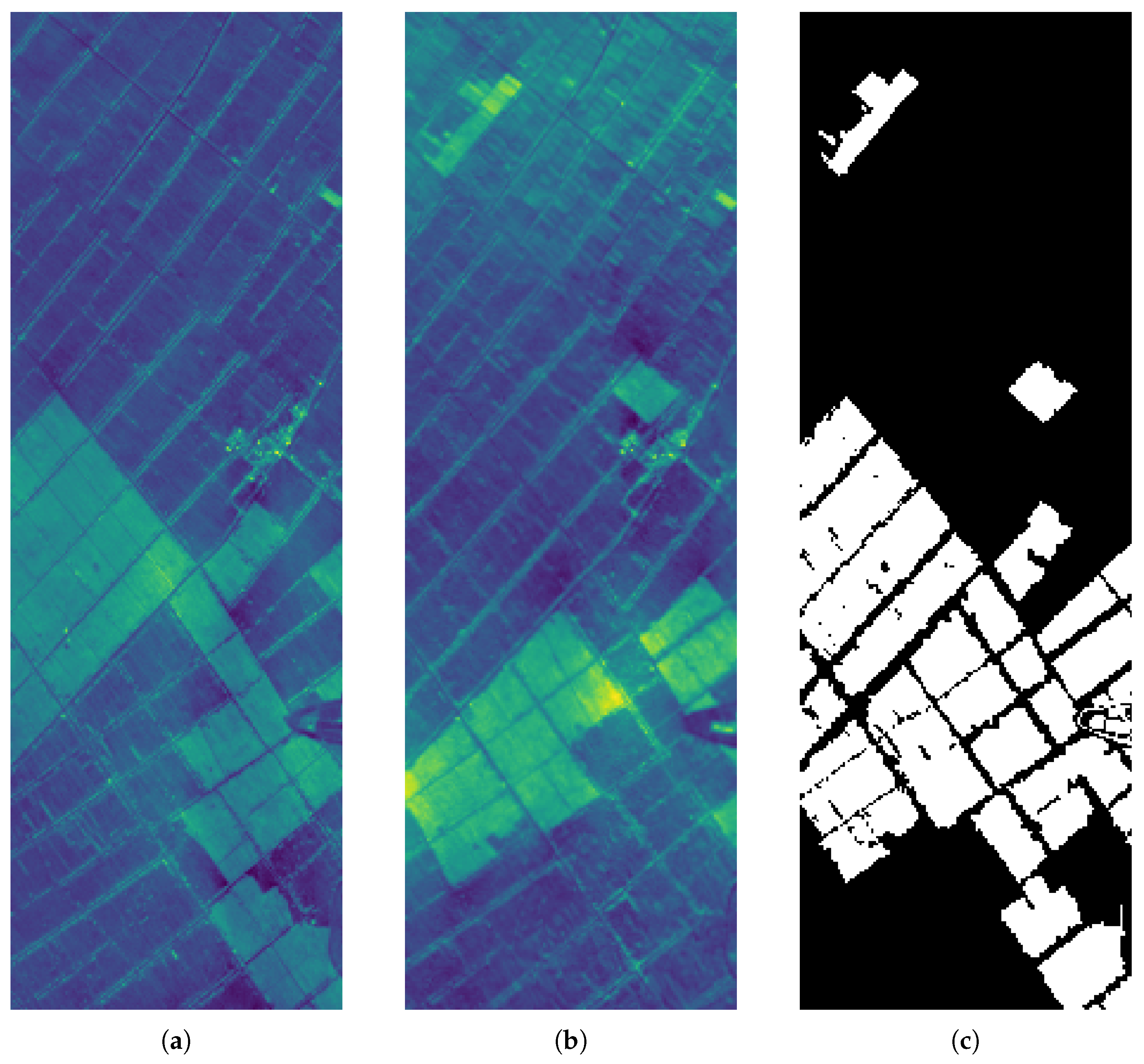
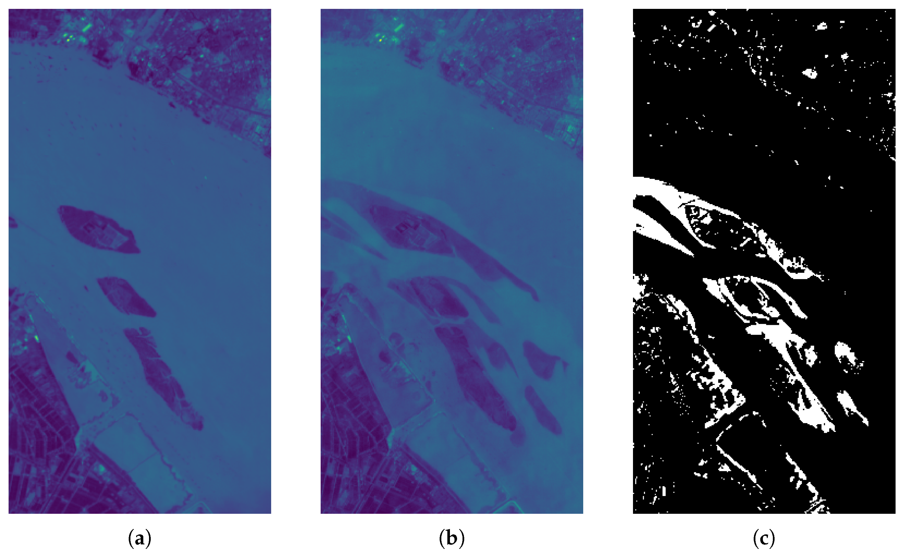
In this review, we use two well-established hyperspectral datasets, Farmland, as shown in Figure 8, and River, as shown in Figure 9, to compare the performance of change detection methods. These datasets are widely adopted in the community because they provide reliable ground-truth maps, which are essential for fair and meaningful evaluation. Without accurate reference labels, performance comparisons can be misleading, and conclusions may lose validity. As shown in Table 3, both datasets are derived from Hyperion imagery collected over Jiangsu Province, China, but they represent very different environments. Farmland covers wetland agricultural regions where changes are driven by vegetation cycles, bare soil exposure, and seasonal water variations. The River dataset, on the other hand, captures fluvial landscapes with shifts shaped by hydrology and land-cover dynamics. Together, they provide complementary testbeds that probe different aspects of spectral and spatial complexity.

Analyzing these datasets are not straightforward. Both are dominated by a large no-change class, making classification imbalanced and harder to generalize. Subtle spectral shifts between vegetation, soil, and water often resemble genuine change, leading to confusion. Added to this, the Hyperion sensor is prone to striping and has a relatively low signal-to-noise ratio, which requires careful preprocessing [133]. Despite these challenges, Farmland and River have become benchmarks for the field, used extensively across supervised, semi-supervised, and unsupervised deep learning approaches.

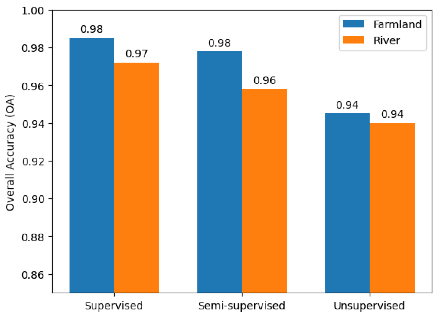
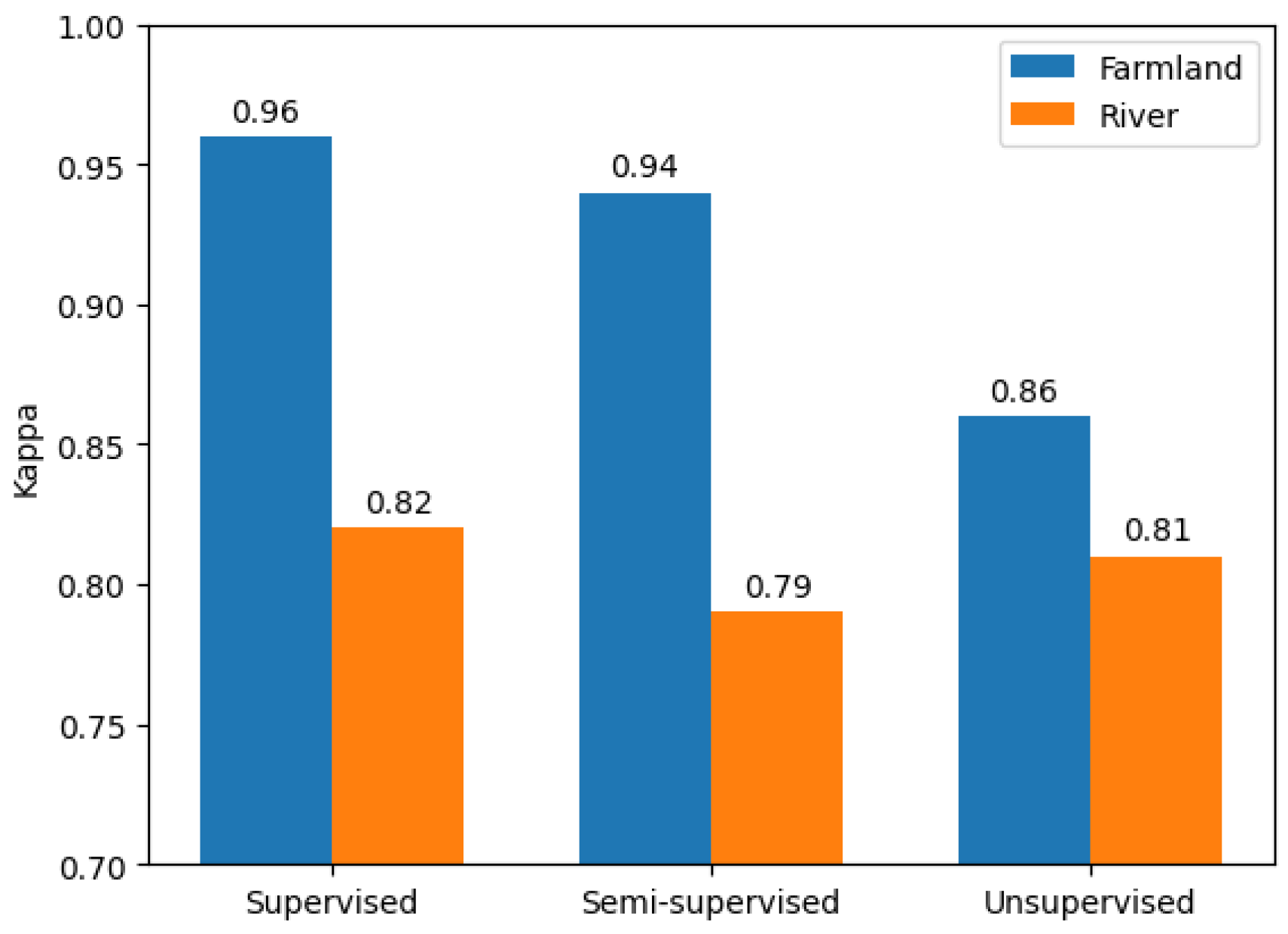
For evaluation, we rely primarily on overall accuracy (OA) and Cohen’s kappa coefficient ($\kappa$). OA reflects the percentage of correctly classified pixels, but it tends to favor the majority class. Kappa provides a more balanced view by accounting for chance agreement, making it particularly useful in highly imbalanced datasets. Taken together, these two measures give a fair basis for comparison across model families and supervision strategies.

Table 4. Comparison of representative HSI-CD methods on the Farmland and River datasets.

Method	Supervision	Model Type	Farmland		River
			OA (%)	Kappa	OA (%)	Kappa
GETNET [61]	Semi-supervised	2D-CNN (mixed affinity + unmixing)	0.9783	0.9572	0.9514	0.7539
TDSSC [62]	Supervised	CNN (1D + 2D spectral–spatial convolutions)	0.9904	0.9759	0.9737	0.8319
SFB-FFGNET [65]	Supervised	CNN (slow-fast band selection + feature fusion grouping)	0.9761	0.9431	0.9671	0.7714
MP-ConvLSTM [69]	Supervised	Multipath ConvLSTM + Siamese CNN + channel attention	0.9889	0.9723	0.9750	0.8443
CSANet [111]	Supervised	Cross-temporal symmetric attention network (Siamese CNN + CSA)	0.9901	0.9751	0.9680	0.7851
SSA-SiamNet [77]	Supervised	Siamese CNN with spectral–spatial attention	0.9787	0.9481	0.9718	0.8053
D2AGCN [103]	Supervised	Dual-branch GCN + difference amplification	0.9374	0.8568	0.9634	0.7931
CODE-HCD [55]	Semi-supervised	GNN + convex optimization	0.9701	0.9271	0.9540	0.7070
CSDBF [104]	Semi-supervised	Graph attention + CNN (dual branch)	0.9843	0.9620	0.9697	0.7982
MGCN [134]	Supervised	Multiorder GCN with channel attention module	0.9662	0.9219	0.9697	0.7982
HMGCF [49]	Supervised	Hybrid GCN + CNN	0.9709	0.9314	0.9763	0.8463
SSIM [135]	Unsupervised	CNN with self-generated credible labels (CVA + SSIM)	0.9746	0.9383	0.9639	0.7403
TSCA [92]	Unsupervised	Two-stream coupled autoencoder + intrinsic decomposition model	0.9731	0.9348	0.9718	0.8582
FGDNet [54]	Unsupervised	Graph domain adaptive network	0.9258	0.8330	0.9239	0.8291
PCPTNet [116]	Unsupervised	Pyramid transfer	0.9294	0.8373	0.9507	0.7318
D2IAR [125]	Unsupervised	Distribution distance with inconsistent adaptive region	0.9736	0.9415	0.9510	0.9141
ABBD [136]	Unsupervised	Band-wise binary distancing	0.8879	0.7427	0.9637	0.7928

presents a representative set of results. While it does not capture every published method, it covers a balanced mix of architectures and supervision levels. Several clear patterns emerge: Supervised CNNs and attention-based networks deliver the highest accuracies, often exceeding 99% OA on Farmland. Semi-supervised graph-based hybrids achieve nearly the same performance with fewer labels, underscoring their practical appeal. Unsupervised methods remain more variable, but advanced designs such as autoencoder-based frameworks and distribution distance measures have narrowed the gap, sometimes reaching the accuracy levels of supervised baselines. Across the board, performance on the River dataset is consistently lower, reflecting its greater spectral complexity and environmental variability.

Dataset effects are also evident. Farmland consistently yields higher accuracies, whereas the River dataset poses more difficulty, leading to reduced OA and $\kappa$ across almost all methods. This suggests that hydrological variability and spectral confusion present tougher conditions for generalization. Overall, while supervised CNN-based models remain state-of-the-art, semi-supervised graph-based hybrids and advanced unsupervised designs are narrowing the gap, pointing toward a more balanced trade-off between accuracy and annotation efficiency.

To highlight these trends more clearly, Figure 10 and Figure 11 illustrate the aggregated OA and $\kappa$ values for supervised, semi-supervised, and unsupervised methods on the two datasets. These visual comparisons reinforce the same conclusions: supervised approaches dominate in benchmark performance, semi-supervised hybrids provide competitive accuracy with reduced annotation requirements, and unsupervised methods, while still trailing, are showing steady improvements. The River dataset consistently yields lower scores than Farmland, underscoring the challenge of spectral complexity in hydrological environments.

Looking at the results in Table 4 together with the averages in Figure 10 and Figure 11, a few patterns become clear. These results not only confirm the strength of supervised CNN and attention-based models but also emphasize the growing competitiveness of semi-supervised and unsupervised designs. Graph-based networks, in particular, stand out for their ability to explicitly model spectral–spatial relationships and capture nonlocal dependencies. Although these approaches often incur higher computational and memory costs due to graph construction and message passing, their performance on challenging datasets demonstrates that the added complexity can pay off in terms of accuracy and robustness. More broadly, the results highlight the importance of the characteristics of the dataset in generalizing the model, reminding us that strong performance on one benchmark does not always translate to others.

8. Discussion of Gaps and Future Directions

While Section 3 discussed current trends and challenges, it is equally important to highlight the broader gaps in the field of HSI-CD that remain underexplored. Addressing these gaps will be the key to shaping the next stage of research. In the following, we summarize the major research gaps and outline possible directions for future work.

• Dataset Diversity and Standardization: A major gap in HSI-CD research is the continued reliance on a small number of benchmark datasets, such as Farmland, River, and Hermiston, which limits the ability to assess model robustness across diverse environmental, spectral, and geographic conditions. In addition, variations in preprocessing pipelines, train-test splits, and evaluation protocols make it difficult to compare methods fairly across studies. Future work should therefore prioritize not only larger and more diverse benchmark datasets but also more standardized evaluation practices, including consistent reporting of OA, Kappa, F1-score, precision, and recall; explicit description of preprocessing steps; and clear documentation of train/validation/test sampling protocols.
• Cross-Sensor and Cross-Region Generalization: Another important gap is the limited transferability of current models across sensors, regions, and acquisition conditions. Many methods perform well only under the specific spectral characteristics and distributions seen during training, which restricts their use in real-world scenarios. Future research should place greater emphasis on domain adaptation, transfer learning, test-time adaptation, and sensor-invariant representation learning to improve cross-domain robustness without requiring full retraining.
• Label Scarcity and Annotation Burden: Despite recent progress in semi-supervised and self-supervised learning, the field still lacks sufficiently label-efficient frameworks that can fully exploit the large volumes of unlabeled hyperspectral data available in practice. Pixel-level annotation remains expensive and time-consuming, which continues to constrain the scale of supervised HSI-CD research. Promising future directions include generative pretraining, foundation-model-style representation learning, active learning, and federated learning, all of which may help reduce annotation demands while preserving strong detection performance.
• Computational Efficiency and Real-Time Deployment: While recent transformer-based and graph-based models have improved representational power, a significant gap remains between algorithmic performance and deployability. Many existing methods are still too computationally intensive for large-scale monitoring, real-time analysis, or onboard processing environments. Future work should therefore focus on lightweight architectures, model compression, pruning, knowledge distillation, and more efficient graph construction and attention mechanisms to enable practical deployment in edge and resource-constrained settings.
• Interpretability and Trustworthiness: Interpretability remains underdeveloped in HSI-CD, even as model complexity continues to increase. Most methods provide limited insight into which spectral, spatial, or temporal cues are driving their predictions, which reduces user trust in safety-critical applications such as disaster monitoring, defense, and environmental assessment. Future research should develop explainable AI techniques specifically tailored to hyperspectral spectral–spatial–temporal representations. For example, gradient-based visualization methods such as Grad-CAM [137] could be adapted to highlight the spatial regions and spectral channels that most strongly influence a predicted change, while feature-attribution methods such as SHAP [138] and LIME could help quantify the relative importance of spectral-spatial features in the model decision process. These directions may help make HSI-CD predictions more transparent, reliable, and easier to validate.
• Integration with Multimodal Data: An additional underexplored gap in HSI-CD is the limited use of multimodal information. Most existing studies focus on hyperspectral imagery alone, even though practical monitoring tasks often involve complementary data sources such as SAR, LiDAR, multispectral imagery, or optical images. These modalities can provide information that is not fully captured by HSI alone. For example, SAR can improve robustness under cloud cover and adverse weather conditions; LiDAR can provide structural and elevation information useful for detecting terrain or urban changes; and multispectral or optical imagery can offer complementary spatial detail and broader temporal coverage. Future research should therefore investigate multimodal fusion strategies that better integrate spectral, structural, spatial, and temporal information to improve robustness, generalization, and performance in complex real-world environments.

9. Conclusions

HSI-CD has advanced rapidly in recent years, fueled by the availability of new airborne and satellite sensors and the adoption of DL methods. In this review, we explore how different neural network families, CNNs, transformers, graph networks, and hybrid models have been adapted to extract the rich spectral–spatial features needed for analyzing multitemporal hyperspectral imagery. Our survey, together with a focused case study, presents a clear picture: supervised models remain the strongest on benchmarks, but they rely heavily on large annotated datasets. Semi-supervised and unsupervised approaches are steadily improving, offering promising alternatives when labeled data are limited. Graph- and transformer-based models are particularly powerful in capturing complex relationships, although their heavy computational requirements remain a barrier. We also found that the results are strongly tied to the data set used, which underscores the need for broader and more standardized benchmarks if fair comparisons and generalizations are to be achieved.

At the same time, there are important research gaps to address. Today’s models often struggle to generalize across sensors and regions, are computationally demanding, and largely act as black boxes, offering little interpretability. Closing these gaps will require building larger and more diverse datasets, designing more efficient and lightweight architectures, and developing methods that can explain their predictions in a way users can trust. Looking ahead, exciting opportunities lie ahead: self-supervised learning, generative pretraining, multimodal fusion with other data sources, and even onboard satellite AI all have the potential to push the field forward. By tackling these challenges, hyperspectral change detection can become an indispensable tool for monitoring ecosystems, supporting disaster response, managing natural resources, and addressing global issues such as climate change.

References

1. Bengio, Y. Learning Deep Architectures for AI. Foundations 2009, 2, 1–127. [Google Scholar] [CrossRef]
2. Goodfellow, I.; Bengio, Y.; Courville, A.; Bengio, Y. Deep Learning; MIT Press: Cambridge, MA, USA, 2016. [Google Scholar]
3. Kufel, J.; Niewiadomska, J.; Zyśko, D.; Śliwczyński, A.; Szymański, P. What Is Machine Learning, Artificial Neural Networks and Deep Learning? Examples of Practical Applications in Medicine. Diagnostics 2023, 13, 2582. [Google Scholar] [CrossRef]
4. Deng, J.S.; Wang, K.; Deng, Y.H.; Qi, G.J. PCA-Based Land-Use Change Detection and Analysis Using Multitemporal and Multisensor Satellite Data. Int. J. Remote Sens. 2008, 29, 4823–4838. [Google Scholar] [CrossRef]
5. Bovolo, F.; Marchesi, S.; Bruzzone, L. A Framework for Automatic and Unsupervised Detection of Multiple Changes in Multitemporal Images. IEEE Trans. Geosci. Remote Sens. 2012, 50, 2196–2212. [Google Scholar] [CrossRef]
6. Johnson, R.D.; Kasischke, E.S. Change Vector Analysis: A Technique for the Multispectral Monitoring of Land Cover and Condition. Int. J. Remote Sens. 1998, 19, 411–426. [Google Scholar] [CrossRef]
7. Hao, M.; Zhou, M.; Jin, J.; Shi, W. An Advanced Superpixel-Based Markov Random Field Model for Unsupervised Change Detection. IEEE Geosci. Remote Sens. Lett. 2020, 17, 1401–1405. [Google Scholar] [CrossRef]
8. Cheng, G.; Huang, Y.; Li, X.; Lyu, S.; Xu, Z.; Zhao, H.; Zhao, Q.; Xiang, S. Change Detection Methods for Remote Sensing in the Last Decade: A Comprehensive Review. Remote Sens. 2024, 16, 2355. [Google Scholar] [CrossRef]
9. Ward, S. CEOS EO Handbook. 2014. Available online: https://eohandbook.com/eohb2012/sat_earth_obs_hyperspectral.html (accessed on 22 May 2025).
10. Lu, B.; Dao, P.D.; Liu, J.; He, Y.; Shang, J. Recent Advances of Hyperspectral Imaging Technology and Applications in Agriculture. Remote Sens. 2020, 12, 2659. [Google Scholar] [CrossRef]
11. SPECIM, Spectral Imaging Ltd. Benefits of Hyperspectral Imaging for Research. Available online: https://www.specim.com/technology/benefits-of-hsi-for-research/ (accessed on 22 May 2025).
12. Folkman, M.A.; Pearlman, J.; Liao, L.B.; Jarecke, P.J. EO-1/Hyperion Hyperspectral Imager Design, Development, Characterization, and Calibration. In Hyperspectral Remote Sensing of the Land and Atmosphere; Smith, W.L., Yasuoka, Y., Eds.; SPIE: Bellingham, WA, USA, 2001; Volume 4151, pp. 40–51. [Google Scholar] [CrossRef]
13. eoPortal. PROBA-1 Satellite Mission. 2025. Available online: https://www.eoportal.org/satellite-missions/proba-1 (accessed on 19 September 2025).
14. Zhong, Y.; Wang, X.; Wang, S.; Zhang, L. Advances in Spaceborne Hyperspectral Remote Sensing in China. Geo-Spat. Inf. Sci. 2021, 24, 95–120. [Google Scholar] [CrossRef]
15. eoPortal. IMS-1 Satellite Mission. 2025. Available online: https://www.eoportal.org/satellite-missions/ims-1 (accessed on 18 September 2025).
16. NASA OceanColor. HICO—Hyperspectral Imager for the Coastal Ocean. 2025. Available online: https://oceancolor.gsfc.nasa.gov/data/hico/ (accessed on 18 September 2025).
17. Ge, X.; Ding, J.; Teng, D.; Xie, B.; Zhang, X.; Wang, J.; Han, L.; Bao, Q.; Wang, J. Exploring the Capability of Gaofen-5 Hyperspectral Data for Assessing Soil Salinity Risks. Int. J. Appl. Earth Obs. Geoinf. 2022, 112, 102969. [Google Scholar] [CrossRef]
18. ASI–Italian Space Agency. PRISMA Mission—Earth Science. 2025. Available online: https://www.asi.it/en/earth-science/prisma/ (accessed on 18 September 2025).
19. Shebl, A.; Abdellatif, M.; Abriha, D.; Dawoud, M.; Hussein Ali, M.A.; Mahmoud, A.S.; Kristály, F.; Csámer, Á. EnMap Hyperspectral Data in Geological Investigations: Evaluation for Lithological and Hydrothermal Alteration Mapping in Neoproterozoic Rocks. Gondwana Res. 2025, 143, 91–124. [Google Scholar] [CrossRef]
20. Lu, H.; Qiao, D.; Li, Y.; Wu, S.; Deng, L. Fusion of China ZY-1 02D Hyperspectral Data and Multispectral Data: Which Methods Should Be Used? Remote Sens. 2021, 13, 2354. [Google Scholar] [CrossRef]
21. Tang, H.; Xiao, C.; Chen, W.; Wu, T. On-Orbit Spectral Calibration and Validation of GF5-02 Advanced Hyperspectral Imager. IEEE Geosci. Remote Sens. Lett. 2025, 22, 5506005. [Google Scholar] [CrossRef]
22. Mahalingam, S.; Srinivas, P.; Devi, P.K.; Sita, D.; Das, S.K.; Leela, T.S.; Venkataraman, V.R. Reflectance Based Vicarious Calibration of HySIS Sensors and Spectral Stability Study over Pseudo-Invariant Sites. In Proceedings of the 2019 IEEE Recent Advances in Geoscience and Remote Sensing: Technologies, Standards and Applications (TENGARSS), Kochi, India, 17–20 October 2019; pp. 132–136. [Google Scholar] [CrossRef]
23. Iwasaki, A.; Ohgi, N.; Tanii, J.; Kawashima, T.; Inada, H. Hyperspectral Imager Suite (HISUI)—Japanese Hyper-Multi Spectral Radiometer. In Proceedings of the 2011 IEEE International Geoscience and Remote Sensing Symposium, Vancouver, BC, Canada, 24–29 July 2011; pp. 1025–1028. [Google Scholar] [CrossRef]
24. Mahlayeye, M.; Darvishzadeh, R.; Jepkosgei, C.; Mlawa, K.A.; Nelson, A. DESIS Hyperspectral Satellite Data for Cropping Pattern Classification. IEEE J. Sel. Top. Appl. Earth Obs. Remote Sens. 2024, 17, 17917–17929. [Google Scholar] [CrossRef]
25. Thompson, D.R.; Green, R.O.; Bradley, C.; Brodrick, P.G.; Mahowald, N.; Ben Dor, E.; Bennett, M.; Bernas, M.; Carmon, N.; Chadwick, K.D.; et al. On-Orbit Calibration and Performance of the EMIT Imaging Spectrometer. Remote Sens. Environ. 2024, 303, 113986. [Google Scholar] [CrossRef]
26. Sanders, L.; Randolph, M.; Bangalore, K.; Spivey, A. Orbital Sidekick Global Hyperspectral Observation Satellite (GHOSt) Payload: Calibration and Characterization. In Infrared Remote Sensing and Instrumentation XXXII; Strojnik, M., Helbert, J., Eds.; SPIE: Bellingham, WA, USA, 2024; Volume 13144, p. 1314408. [Google Scholar] [CrossRef]
27. Qin, H.; Wang, W.; Yao, Y.; Qian, Y.; Xiong, X.; Zhou, W. First Experience with Zhuhai-1 Hyperspectral Data for Urban Dominant Tree Species Classification in Shenzhen, China. Remote Sens. 2023, 15, 3179. [Google Scholar] [CrossRef]
28. Duren, R.; Cusworth, D.; Ayasse, A.; Howell, K.; Diamond, A.; Scarpelli, T.; Kim, J.; O’neill, K.; Lai-Norling, J.; Thorpe, A.; et al. The Carbon Mapper Emissions Monitoring System. EGUsphere 2025, 18, 6933–6958. [Google Scholar] [CrossRef]
29. Malila, W.A. Change Vector Analysis: An Approach for Detecting Forest Changes with Landsat. In Proceedings of the 6th Annual Symposium on Machine Processing of Remotely Sensed Data; Purdue University, Laboratory for Applications of Remote Sensing: West Lafayette, IN, USA, 1980; pp. 326–335. [Google Scholar]
30. Fung, T.; LeDrew, E.F. Application of Principal Components Analysis to Change Detection. Photogramm. Eng. Remote Sens. 1987, 53, 1649–1658. [Google Scholar]
31. Nielsen, A.A.; Conradsen, K.; Simpson, J.J. Multivariate Alteration Detection (MAD) and MAF Postprocessing in Multispectral, Bitemporal Image Data: New Approaches to Change Detection Studies. Remote Sens. Environ. 1998, 64, 1–19. [Google Scholar] [CrossRef]
32. Bruzzone, L.; Prieto, D.F. Automatic Analysis of the Difference Image for Unsupervised Change Detection. IEEE Trans. Geosci. Remote Sens. 2000, 38, 1171–1182. [Google Scholar] [CrossRef]
33. Bazi, Y.; Bruzzone, L.; Melgani, F. An Unsupervised Approach Based on the Generalized Gaussian Model to Automatic Change Detection in Multitemporal SAR Images. IEEE Trans. Geosci. Remote Sens. 2005, 43, 874–887. [Google Scholar] [CrossRef]
34. Celik, T. Unsupervised Change Detection in Satellite Images Using Principal Component Analysis and k-Means Clustering. IEEE Geosci. Remote Sens. Lett. 2009, 6, 772–776. [Google Scholar] [CrossRef]
35. Ghosh, S.; Bruzzone, L.; Patra, S.; Bovolo, F.; Ghosh, A. A Context-Sensitive Technique for Unsupervised Change Detection Based on Hopfield-Type Neural Networks. IEEE Trans. Geosci. Remote Sens. 2007, 45, 778–789. [Google Scholar] [CrossRef]
36. Volpi, M.; Tuia, D.; Camps-Valls, G.; Kanevski, M. Unsupervised Change Detection in the Feature Space Using Kernels. In Proceedings of the 2011 IEEE International Geoscience and Remote Sensing Symposium, Vancouver, BC, Canada, 24–29 July 2011; pp. 106–109. [Google Scholar] [CrossRef]
37. Fazel, M.A.; Poncos, V.; Homayouni, S.; Motagh, M. Land Cover Change Detection Using Unsupervised Kernel C-Means and Multi-Temporal SAR Data. In Proceedings of the 2013 IEEE International Geoscience and Remote Sensing Symposium (IGARSS), Melbourne, VIC, Australia, 21–26 July 2013; pp. 2744–2747. [Google Scholar] [CrossRef]
38. Singh, A. Review Article: Digital Change Detection Techniques Using Remotely-Sensed Data. Int. J. Remote Sens. 1989, 10, 989–1003. [Google Scholar] [CrossRef]
39. Ridd, M.K.; Liu, J. A Comparison of Four Algorithms for Change Detection in an Urban Environment. Remote Sens. Environ. 1998, 63, 95–100. [Google Scholar] [CrossRef]
40. Dahiya, N.; Singh, S.; Gupta, S.; Rajab, A.; Hamdi, M.; Elmagzoub, M.A.; Sulaiman, A.; Shaikh, A. Detection of Multitemporal Changes with Artificial Neural Network-Based Change Detection Algorithm Using Hyperspectral Dataset. Remote Sens. 2023, 15, 1326. [Google Scholar] [CrossRef]
41. Yu, H.; Yang, H.; Gao, L.; Hu, J.; Plaza, A.; Zhang, B. Hyperspectral Image Change Detection Based on Gated Spectral–Spatial–Temporal Attention Network with Spectral Similarity Filtering. IEEE Trans. Geosci. Remote Sens. 2024, 62, 5511313. [Google Scholar] [CrossRef]
42. Seydi, S.T.; Hasanlou, M. A New Structure for Binary and Multiple Hyperspectral Change Detection Based on Spectral Unmixing and Convolutional Neural Network. Measurement 2021, 186, 110137. [Google Scholar] [CrossRef]
43. Song, B.; Wu, Z.; Xu, Y.; Xia, X.; Xie, Y.; Zhan, T.; Wei, Z. 3DCNN-NF: Few-Shot Hyperspectral Image Change Detection Based on 3-D Convolution Neural Network and Normalizing Flow. IEEE Trans. Geosci. Remote Sens. 2024, 62, 5530615. [Google Scholar] [CrossRef]
44. Zhang, Y.; Zhang, M.; Li, W.; Wang, S.; Tao, R. Language-Aware Domain Generalization Network for Cross-Scene Hyperspectral Image Classification. IEEE Trans. Geosci. Remote Sens. 2023, 61, 5501312. [Google Scholar] [CrossRef]
45. Seydi, S.T.; Boueshagh, M.; Namjoo, F.; Minouei, S.M.; Nikraftar, Z.; Amani, M. A Hyperspectral Change Detection (HCD-Net) Framework Based on Double Stream Convolutional Neural Networks and an Attention Module. Remote Sens. 2024, 16, 827. [Google Scholar] [CrossRef]
46. Wen, D.; Jiang, Y.; Chen, D.; Tian, Y. Fusion of Bi-Temporal Zhuhai-1 Orbita Hyperspectral and Multiseason Sentinel-2 Remote Sensing Imagery for Semantic Change Detection Based on Dual-Path 3DCNN-LSTM. IEEE Geosci. Remote Sens. Lett. 2025, 22, 6003005. [Google Scholar] [CrossRef]
47. Zhang, X.; Tian, S.; Wang, G.; Tang, X.; Feng, J.; Jiao, L. CAST: A Cascade Spectral-Aware Transformer for Hyperspectral Image Change Detection. IEEE Trans. Geosci. Remote Sens. 2023, 61, 5520714. [Google Scholar] [CrossRef]
48. Zhang, W.; Su, L.; Zhang, Y.; Lu, X. A Spectrum-Aware Transformer Network for Change Detection in Hyperspectral Imagery. IEEE Trans. Geosci. Remote Sens. 2023, 61, 5518612. [Google Scholar] [CrossRef]
49. Katiyar, C.; Manian, V. Hyperspectral Multilevel GCN and CNN Feature Fusion for Change Detection. IEEE J. Sel. Top. Appl. Earth Obs. Remote Sens. 2024, 17, 19146–19159. [Google Scholar] [CrossRef]
50. Zheng, X.; Lin, X.; Qing, L.; Ou, X. Semantic-Aware Remote Sensing Change Detection with Multi-Scale Cross-Attention. Sensors 2025, 25, 2813. [Google Scholar] [CrossRef]
51. Zhang, Y.; Wang, T.; Zhang, C.; Xu, S.; Gao, H.; Li, C. A Dual-Branch Siamese Spatial-Spectral Transformer Attention Network for Hyperspectral Image Change Detection. Expert Syst. Appl. 2024, 238, 122125. [Google Scholar] [CrossRef]
52. Tong, X.; Pan, H.; Liu, S.; Li, B.; Luo, X.; Xie, H.; Xu, X. A Novel Approach for Hyperspectral Change Detection Based on Uncertain Area Analysis and Improved Transfer Learning. IEEE J. Sel. Top. Appl. Earth Obs. Remote Sens. 2020, 13, 2056–2069. [Google Scholar] [CrossRef]
53. Hu, M.; Wu, C.; Zhang, L. HyperNet: Self-Supervised Hyperspectral Spatial–Spectral Feature Understanding Network for Hyperspectral Change Detection. IEEE Trans. Geosci. Remote Sens. 2022, 60, 5543017. [Google Scholar] [CrossRef]
54. Qu, J.; Zhao, J.; Dong, W.; Xiao, S.; Li, Y.; Du, Q. Feature Mutual Representation-Based Graph Domain Adaptive Network for Unsupervised Hyperspectral Change Detection. IEEE Trans. Geosci. Remote Sens. 2024, 62, 5501214. [Google Scholar] [CrossRef]
55. Lin, T.-H.; Lin, C.-H. Hyperspectral Change Detection Using Semi-Supervised Graph Neural Network and Convex Deep Learning. IEEE Trans. Geosci. Remote Sens. 2023, 61, 5515818. [Google Scholar] [CrossRef]
56. Liu, S.; Marinelli, D.; Bruzzone, L.; Bovolo, F. A Review of Change Detection in Multitemporal Hyperspectral Images: Current Techniques, Applications, and Challenges. IEEE Geosci. Remote Sens. Mag. 2019, 7, 140–158. [Google Scholar] [CrossRef]
57. Shafique, A.; Cao, G.; Khan, Z.; Asad, M.; Aslam, M. Deep Learning-Based Change Detection in Remote Sensing Images: A Review. Remote Sens. 2022, 14, 871. [Google Scholar] [CrossRef]
58. Hu, M.; Wu, C.; Du, B. Multi-Temporal Spatial-Spectral Comparison Network For Hyperspectral Anomalous Change Detection. In Proceedings of the IGARSS 2022—2022 IEEE International Geoscience and Remote Sensing Symposium, Kuala Lumpur, Malaysia, 17–22 July 2022; pp. 1432–1435. [Google Scholar] [CrossRef]
59. Lenail, A. NN-SVG: Publication-Ready Neural Network Architecture Schematics. 2024; Accessed for Figure Generation. Available online: https://alexlenail.me/NN-SVG/ (accessed on 5 January 2026).
60. Boureau, Y.-L.; Ponce, J.; LeCun, Y. A Theoretical Analysis of Feature Pooling in Visual Recognition. In Proceedings of the 27th International Conference on Machine Learning, Haifa, Israel, 21–24 June 2010; pp. 111–118. [Google Scholar]
61. Wang, Q.; Yuan, Z.; Du, Q.; Li, X. GETNET: A General End-to-End 2-D CNN Framework for Hyperspectral Image Change Detection. IEEE Trans. Geosci. Remote Sens. 2019, 57, 3–13. [Google Scholar] [CrossRef]
62. Zhan, T.; Song, B.; Sun, L.; Jia, X.; Wan, M.; Yang, G.; Wu, Z. TDSSC: A Three-Directions Spectral–Spatial Convolution Neural Network for Hyperspectral Image Change Detection. IEEE J. Sel. Top. Appl. Earth Obs. Remote Sens. 2021, 14, 377–388. [Google Scholar] [CrossRef]
63. Yuan, Z.; Wang, Q.; Li, X. ROBUST PCANet for Hyperspectral Image Change Detection. In Proceedings of the IGARSS 2018—2018 IEEE International Geoscience and Remote Sensing Symposium, Valencia, Spain, 22–27 July 2018; pp. 4931–4934. [Google Scholar] [CrossRef]
64. Wang, X.; Xing, C.; Feng, Y.; Song, R.; Mu, Z. A Novel Hyperspectral Image Change Detection Framework Based on 3D-Wavelet Domain Active Convolutional Neural Network. In Proceedings of the 2021 IEEE International Geoscience and Remote Sensing Symposium IGARSS, Brussels, Belgium, 11–16 July 2021; pp. 4332–4335. [Google Scholar] [CrossRef]
65. Ou, X.; Liu, L.; Tu, B.; Zhang, G.; Xu, Z. A CNN Framework with Slow-Fast Band Selection and Feature Fusion Grouping for Hyperspectral Image Change Detection. IEEE Trans. Geosci. Remote Sens. 2022, 60, 5524716. [Google Scholar] [CrossRef]
66. Wang, L.; Wang, L.; Wang, Q.; Bruzzone, L. RSCNet: A Residual Self-Calibrated Network for Hyperspectral Image Change Detection. IEEE Trans. Geosci. Remote Sens. 2022, 60, 5529917. [Google Scholar] [CrossRef]
67. Yang, Y.; Qu, J.; Xiao, S.; Dong, W.; Li, Y.; Du, Q. A Deep Multiscale Pyramid Network Enhanced with Spatial–Spectral Residual Attention for Hyperspectral Image Change Detection. IEEE Trans. Geosci. Remote Sens. 2022, 60, 5525513. [Google Scholar] [CrossRef]
68. Qu, J.; Hou, S.; Dong, W.; Li, Y.; Xie, W. A Multilevel Encoder–Decoder Attention Network for Change Detection in Hyperspectral Images. IEEE Trans. Geosci. Remote Sens. 2022, 60, 5518113. [Google Scholar] [CrossRef]
69. Shi, C.; Zhang, Z.; Zhang, W.; Zhang, C.; Xu, Q. Learning Multiscale Temporal–Spatial–Spectral Features via a Multipath Convolutional LSTM Neural Network for Change Detection with Hyperspectral Images. IEEE Trans. Geosci. Remote Sens. 2022, 60, 5529816. [Google Scholar] [CrossRef]
70. Shi, J.; Zhang, Z.; Wu, T.; Zhang, X.; Lei, Y. Collaborative Self-Perception Network Architecture for Hyperspectral Image Change Detection. IEEE Geosci. Remote Sens. Lett. 2022, 19, 5512305. [Google Scholar] [CrossRef]
71. Tang, Y.; Fan, Y.; Feng, S.; Zhao, C.; Luo, T. Hyperspectral Image Change Detection Based on Multi-Scale 3D Convolution Autoencoder. In Proceedings of the IGARSS 2022—2022 IEEE International Geoscience and Remote Sensing Symposium, Kuala Lumpur, Malaysia, 17–22 July 2022; pp. 3211–3214. [Google Scholar] [CrossRef]
72. Ou, X.; Liu, L.; Tan, S.; Zhang, G.; Li, W.; Tu, B. A Hyperspectral Image Change Detection Framework with Self-Supervised Contrastive Learning Pretrained Model. IEEE J. Sel. Top. Appl. Earth Obs. Remote Sens. 2022, 15, 7724–7740. [Google Scholar] [CrossRef]
73. Ge, H.; Tang, Y.; Bi, Z.; Zhan, T.; Xu, Y.; Song, A. MMSRC: A Multidirection Multiscale Spectral–Spatial Residual Network for Hyperspectral Multiclass Change Detection. IEEE J. Sel. Top. Appl. Earth Obs. Remote Sens. 2022, 15, 9254–9265. [Google Scholar] [CrossRef]
74. Shammi, S.A.; Du, Q. Hyperspectral Image Change Detection Using Deep Learning and Band Expansion. In Proceedings of the 2022 12th Workshop on Hyperspectral Imaging and Signal Processing: Evolution in Remote Sensing (WHISPERS), Rome, Italy, 24–27 October 2022; pp. 1–5. [Google Scholar] [CrossRef]
75. Wang, L.; Wang, L.; Wang, H.; Wang, X.; Bruzzone, L. SPCNet: A Subpixel Convolution-Based Change Detection Network for Hyperspectral Images with Different Spatial Resolutions. IEEE Trans. Geosci. Remote Sens. 2022, 60, 5533314. [Google Scholar] [CrossRef]
76. Wang, L.; Wan, L.; Bruzzone, L. A Sub-Pixel Convolution-Based Residual Network for Hyperspectral Image Change Detection. In Proceedings of the IGARSS 2022—2022 IEEE International Geoscience and Remote Sensing Symposium, Kuala Lumpur, Malaysia, 17–22 July 2022; pp. 1059–1062. [Google Scholar] [CrossRef]
77. Wang, L.; Wang, L.; Wang, Q.; Atkinson, P.M. SSA-SiamNet: Spectral–Spatial-Wise Attention-Based Siamese Network for Hyperspectral Image Change Detection. IEEE Trans. Geosci. Remote Sens. 2022, 60, 5533314. [Google Scholar] [CrossRef]
78. Bobate, N.; Yadav, P.P.; Narasimhadhan, A.V. Fusing Conventional and Deep Learning Features for Hyperspectral Image Change Detection. In Proceedings of the 2022 IEEE International Conference on Electronics, Computing and Communication Technologies (CONECCT), Bengaluru, India, 8–10 July 2022; pp. 1–6. [Google Scholar] [CrossRef]
79. Guan, M.; Cho, S.; Petro, R.; Zhang, W.; Pasche, B.; Topaloglu, U. Natural Language Processing and Recurrent Network Models for Identifying Genomic Mutation-Associated Cancer Treatment Change from Patient Progress Notes. JAMIA Open 2019, 2, 139–149. [Google Scholar] [CrossRef]
80. Mienye, I.D.; Swart, T.G.; Obaido, G. Recurrent Neural Networks: A Comprehensive Review of Architectures, Variants, and Applications. Information 2024, 15, 517. [Google Scholar] [CrossRef]
81. Li, X.; Ding, J. Spectral–Temporal Transformer for Hyperspectral Image Change Detection. Remote Sens. 2023, 15, 3561. [Google Scholar] [CrossRef]
82. Hochreiter, S.; Schmidhuber, J. Long Short-Term Memory. Neural Comput. 1997, 9, 1735–1780. [Google Scholar] [CrossRef]
83. Lyu, H.; Lu, H.; Mou, L. Learning a Transferable Change Rule from a Recurrent Neural Network for Land Cover Change Detection. Remote Sens. 2016, 8, 506. [Google Scholar] [CrossRef]
84. Song, A.; Choi, J.; Han, Y.; Kim, Y. Change Detection in Hyperspectral Images Using Recurrent 3D Fully Convolutional Networks. Remote Sens. 2018, 10, 1827. [Google Scholar] [CrossRef]
85. Miao, Z.; Lin, Z.; Jia, P.; Shen, Y. Change Detection Method for Hyperspectral Image with Sequential Time Series Inputs. In Proceedings of the 2017 36th Chinese Control Conference (CCC), Dalian, China, 26–28 July 2017; pp. 10819–10822. [Google Scholar] [CrossRef]
86. Rumelhart, D.E.; Hinton, G.E.; Williams, R.J. Learning Internal Representations by Error Propagation. In Parallel Distributed Processing: Explorations in the Microstructure of Cognition, Vol. 1: Foundations; MIT Press: Cambridge, MA, USA, 1986; pp. 318–362. [Google Scholar]
87. Hinton, G.E.; Salakhutdinov, R.R. Reducing the Dimensionality of Data with Neural Networks. Science 2006, 313, 504–507. [Google Scholar] [CrossRef] [PubMed]
88. Vincent, P.; Larochelle, H.; Bengio, Y.; Manzagol, P.-A. Extracting and Composing Robust Features with Denoising Autoencoders. In Proceedings of the 25th International Conference on Machine Learning, Helsinki, Finland, 5–9 July 2008; pp. 1096–1103. [Google Scholar] [CrossRef]
89. Zhou, F.; Chen, Z. Hyperspectral Image Change Detection by Self-Supervised Tensor Network. In Proceedings of the IGARSS 2020—2020 IEEE International Geoscience and Remote Sensing Symposium, Waikoloa, HI, USA, 26–31 July 2020; pp. 2527–2530. [Google Scholar] [CrossRef]
90. Hu, M.; Wu, C.; Zhang, L.; Du, B. Hyperspectral Anomaly Change Detection Based on Autoencoder. IEEE J. Sel. Top. Appl. Earth Obs. Remote Sens. 2021, 14, 3750–3762. [Google Scholar] [CrossRef]
91. Wu, H.; Chen, Z. Self-Supervised Confident Learning For Hyperspectral Image Change Detection. In Proceedings of the 2022 12th Workshop on Hyperspectral Imaging and Signal Processing: Evolution in Remote Sensing (WHISPERS), Rome, Italy, 24–27 October 2022; pp. 1–4. [Google Scholar] [CrossRef]
92. Sun, J.; Liu, J.; Xiao, L. Intrinsic Decomposition Model-Guided Two-Stream Coupled Autoencoder for Unsupervised Hyperspectral Image Change Detection. IEEE Geosci. Remote Sens. Lett. 2023, 20, 5503805. [Google Scholar] [CrossRef]
93. Zhao, J.; Xiao, S.; Dong, W.; Qu, J.; Li, Y. Dictionary Learning-Guided Deep Interpretable Network for Hyperspectral Change Detection. IEEE Geosci. Remote Sens. Lett. 2023, 20, 5508405. [Google Scholar] [CrossRef]
94. Qu, J.; Yang, P.; Dong, W.; Zhang, X.; Li, Y. A Semi-Supervised Multiscale Convolutional Sparse Coding-Guided Deep Interpretable Network for Hyperspectral Image Change Detection. IEEE Trans. Geosci. Remote Sens. 2024, 62, 5531314. [Google Scholar] [CrossRef]
95. Goodfellow, I.J.; Pouget-Abadie, J.; Mirza, M.; Xu, B.; Warde-Farley, D.; Ozair, S.; Courville, A.; Bengio, Y. Generative Adversarial Networks. arXiv 2014, arXiv:1406.2661. [Google Scholar] [CrossRef]
96. Mirza, M.; Osindero, S. Conditional Generative Adversarial Nets. arXiv 2014, arXiv:1411.1784. [Google Scholar] [CrossRef]
97. Zhu, J.-Y.; Park, T.; Isola, P.; Efros, A.A. Unpaired Image-to-Image Translation Using Cycle-Consistent Adversarial Networks. arXiv 2020, arXiv:1703.10593. [Google Scholar]
98. Arjovsky, M.; Chintala, S.; Bottou, L. Wasserstein GAN. arXiv 2017, arXiv:1701.07875. [Google Scholar]
99. Lei, J.; Li, M.; Xie, W.; Li, Y.; Jia, X. Spectral Mapping with Adversarial Learning for Unsupervised Hyperspectral Change Detection. Neurocomputing 2021, 465, 71–83. [Google Scholar] [CrossRef]
100. Oubara, A.; Wu, F.; Qu, G.; Maleki, R.; Yang, G. Enhancing Binary Change Detection in Hyperspectral Images Using an Efficient Dimensionality Reduction Technique Within Adversarial Learning. Remote Sens. 2025, 17, 5. [Google Scholar] [CrossRef]
101. Zhang, S.; Deng, Q.; Ding, Z. Multilayer Graph Spectral Analysis for Hyperspectral Images. EURASIP J. Adv. Signal Process. 2022, 2022, 92. [Google Scholar] [CrossRef]
102. Feng, Y.; Ni, W.; Song, L.; Wang, X. MsFNet: Multi-Scale Fusion Network Based on Dynamic Spectral Features for Multi-Temporal Hyperspectral Image Change Detection. Remote Sens. 2024, 16, 3037. [Google Scholar] [CrossRef]
103. Qu, J.; Xu, Y.; Dong, W.; Li, Y.; Du, Q. Dual-Branch Difference Amplification Graph Convolutional Network for Hyperspectral Image Change Detection. IEEE Trans. Geosci. Remote Sens. 2022, 60, 5519912. [Google Scholar] [CrossRef]
104. Wang, X.; Zhao, K.; Zhao, X.; Li, S. CSDBF: Dual-Branch Framework Based on Temporal–Spatial Joint Graph Attention with Complement Strategy for Hyperspectral Image Change Detection. IEEE Trans. Geosci. Remote Sens. 2022, 60, 5540118. [Google Scholar] [CrossRef]
105. Lin, T.-H.; Lin, C.-H.; Young, S.-S. GNN-Based Small-Data Learning with Area-Control Mechanism for Hyperspectral Satellite Change Detection. In Proceedings of the 2023 Asia Pacific Signal and Information Processing Association Annual Summit and Conference (APSIPA ASC), Xiamen, China, 26–29 November 2023; pp. 726–732. [Google Scholar] [CrossRef]
106. Zhao, X.; Li, S.; Geng, T.; Wang, X. GTransCD: Graph Transformer-Guided Multitemporal Information United Framework for Hyperspectral Image Change Detection. IEEE Trans. Geosci. Remote Sens. 2024, 62, 5500313. [Google Scholar] [CrossRef]
107. Lin, C.-H.; Lin, T.-H.; Chanussot, J. Quantum Information-Empowered Graph Neural Network for Hyperspectral Change Detection. IEEE Trans. Geosci. Remote Sens. 2024, 62, 5537615. [Google Scholar] [CrossRef]
108. Vaswani, A.; Shazeer, N.; Parmar, N.; Uszkoreit, J.; Jones, L.; Gomez, A.N.; Kaiser, L.; Polosukhin, I. Attention Is All You Need. arXiv 2023, arXiv:1706.03762. [Google Scholar]
109. Dosovitskiy, A.; Beyer, L.; Kolesnikov, A.; Weissenborn, D.; Zhai, X.; Unterthiner, T.; Dehghani, M.; Minderer, M.; Heigold, G.; Gelly, S.; et al. An Image Is Worth 16x16 Words: Transformers for Image Recognition at Scale. arXiv 2021, arXiv:2010.11929. [Google Scholar] [CrossRef]
110. Ding, J.; Li, X.; Zhao, L. CDFormer: A Hyperspectral Image Change Detection Method Based on Transformer Encoders. IEEE Geosci. Remote Sens. Lett. 2022, 19, 6015405. [Google Scholar] [CrossRef]
111. Song, R.; Ni, W.; Cheng, W.; Wang, X. CSANet: Cross-Temporal Interaction Symmetric Attention Network for Hyperspectral Image Change Detection. IEEE Geosci. Remote Sens. Lett. 2022, 19, 6010105. [Google Scholar] [CrossRef]
112. Dong, W.; Zhao, J.; Qu, J.; Xiao, S.; Li, N.; Hou, S.; Li, Y. Abundance Matrix Correlation Analysis Network Based on Hierarchical Multihead Self-Cross-Hybrid Attention for Hyperspectral Change Detection. IEEE Trans. Geosci. Remote Sens. 2023, 61, 5501513. [Google Scholar] [CrossRef]
113. Shafique, A.; Seydi, S.T.; Alipour-Fard, T.; Cao, G.; Yang, D. SSViT-HCD: A Spatial–Spectral Convolutional Vision Transformer for Hyperspectral Change Detection. IEEE J. Sel. Top. Appl. Earth Obs. Remote Sens. 2023, 16, 6487–6504. [Google Scholar] [CrossRef]
114. Wang, X.; Zhao, K.; Zhao, X.; Li, S. TriTF: A Triplet Transformer Framework Based on Parents and Brother Attention for Hyperspectral Image Change Detection. IEEE Trans. Geosci. Remote Sens. 2023, 61, 5501513. [Google Scholar] [CrossRef]
115. Zhang, W.; Zhang, Y.; Gao, S.; Lu, X.; Tang, Y.; Liu, S. Spectrum-Induced Transformer-Based Feature Learning for Multiple Change Detection in Hyperspectral Images. IEEE Trans. Geosci. Remote Sens. 2024, 62, 5500212. [Google Scholar] [CrossRef]
116. Xu, Y.; Xiao, S.; Qu, J.; Dong, W.; Li, Y.; Xia, H. Parallel Compared-and-Stacked Pyramid Transformer Network for Unsupervised Hyperspectral Change Detection. IEEE Trans. Geosci. Remote Sens. 2024, 62, 5501814. [Google Scholar] [CrossRef]
117. Chen, Y.; Zhang, Z.; Dong, L.; Xiong, S.; Lu, X. A Joint Saliency Temporal–Spatial–Spectral Information Network for Hyperspectral Image Change Detection. IEEE Trans. Geosci. Remote Sens. 2024, 62, 5502315. [Google Scholar] [CrossRef]
118. Huang, Y.; Zhang, L.; Cen, Y.; Song, R.; Qi, W.; Huang, C. Exploring Conflict-Matching Learning with Temporal Weight-Sharing and Bandwise Spatial-Interacting Transformer for Hyperspectral Change Detection. IEEE Trans. Geosci. Remote Sens. 2024, 62, 5531916. [Google Scholar] [CrossRef]
119. Bidari, I.; Chickerur, S.; Kulkarni, A.; Mahajan, A.; Nikkam, A.; Akella, S. Change Detection and Classification Using Hyperspectral Imagery. In Proceedings of the 2021 2nd International Conference on Range Technology (ICORT), Xi’an, China, 15–17 October 2021; pp. 1–6. [Google Scholar] [CrossRef]
120. Ou, X.; Liu, L.; Tu, B.; Qing, L.; Zhang, G.; Liang, Z. CBW-MSSANet: A CNN Framework with Compact Band Weighting and Multiscale Spatial Attention for Hyperspectral Image Change Detection. IEEE Trans. Geosci. Remote Sens. 2023, 61, 5507618. [Google Scholar] [CrossRef]
121. Qiu, S.; Li, C.; Feng, Y.; Liang, H.; Xu, A. CBANet: Context Balancing Attention Network for Rapid Skin Lesion Segmentation. In Proceedings of the 2022 China Automation Congress (CAC), Xiamen, China, 25–27 November, 2022; pp. 4533–4538. [Google Scholar] [CrossRef]
122. Hu, M.; Wu, C.; Du, B.; Zhang, L. Binary Change Guided Hyperspectral Multiclass Change Detection. IEEE Trans. Image Process. 2023, 32, 791–806. [Google Scholar] [CrossRef]
123. Xu, S.; Cai, L.; Sun, H.; Sun, X.; Yang, L.; Gao, L. Adaptive Endmembers Learning-Based Deep Unmixing Network for Hyperspectral Change Detection. In Proceedings of the IGARSS 2024—2024 IEEE International Geoscience and Remote Sensing Symposium, Athens, Greece, 7–12 July, 2024; pp. 10333–10337. [Google Scholar] [CrossRef]
124. Yadav, P.P.; Bobate, N.; Shetty, A.; Raghavendra, B.S.; Narasimhadhan, A.V. ATGP Based Change Detection in Hyperspectral Images. In Proceedings of the IECON 2022—48th Annual Conference of the IEEE Industrial Electronics Society, Brussels, Belgium, 17–20 October 2022; pp. 1–6. [Google Scholar] [CrossRef]
125. Lv, Z.; Lei, Z.; Xie, L.; Falco, N.; Shi, C.; You, Z. Novel Distribution Distance Based on Inconsistent Adaptive Region for Change Detection Using Hyperspectral Remote Sensing Images. IEEE Trans. Geosci. Remote Sens. 2024, 62, 5507618. [Google Scholar] [CrossRef]
126. Yang, B.; Mao, Y.; Liu, L.; Fang, L.; Liu, X. Change Representation and Extraction in Stripes: Rethinking Unsupervised Hyperspectral Image Change Detection with an Untrained Network. IEEE Trans. Image Process. 2024, 33, 5098–5113. [Google Scholar] [CrossRef]
127. Wang, Y.; Sha, J.; Gao, L.; Zhang, Y.; Rong, X.; Zhang, C. A Semi-Supervised Domain Alignment Transformer for Hyperspectral Images Change Detection. IEEE Trans. Geosci. Remote Sens. 2023, 61, 5525411. [Google Scholar] [CrossRef]
128. Xie, W.; Xu, X.; Li, Y. Decentralized Federated GAN for Hyperspectral Change Detection in Edge Computing. IEEE J. Sel. Top. Appl. Earth Obs. Remote Sens. 2024, 17, 8863–8874. [Google Scholar] [CrossRef]
129. Yang, B.; Cheng, X.; Chen, W.; Ye, X. A Graph-Based Hyperspectral Change Detection Framework Using Difference Augmentation and Progressive Reconstruction with Limited Labels. IEEE Trans. Geosci. Remote Sens. 2024, 62, 5518914. [Google Scholar] [CrossRef]
130. Zhao, X.; Li, S.; Liu, X.; Song, C.; Wang, X. Patch- and Class-Wise Hyperspectral Knowledge Learning: A Composite Consistency-Constrained Self-Ensemble Framework for Change Detection. IEEE Trans. Geosci. Remote Sens. 2025, 63, 5509113. [Google Scholar] [CrossRef]
131. Wang, Y.; Sha, J.; Yu, X.; Gao, Y.; Zhang, Y.; Rong, X. A generative pretrained transformer for semi-supervised hyperspectral image change detection. IEEE Geosci. Remote Sens. Lett. 2025, 22, 5502605. [Google Scholar] [CrossRef]
132. Grupo Hiperespectral. ChangeDetectionDataset: Bay Area. 2025. Available online: https://gitlab.citius.gal/hiperespectral/ChangeDetectionDataset/tree/master/bayArea (accessed on 25 September 2025).
133. Campbell, P.K.E.; Middleton, E.M.; Thome, K.J.; Kokaly, R.F.; Huemmrich, K.F.; Lagomasino, D.; Novick, K.A.; Brunsell, N.A. EO-1 Hyperion Reflectance Time Series at Calibration and Validation Sites: Stability and Sensitivity to Seasonal Dynamics. IEEE J. Sel. Top. Appl. Earth Obs. Remote Sens. 2013, 6, 276–290. [Google Scholar] [CrossRef]
134. Zhang, Y.; Miao, R.; Dong, Y.; Du, B. Multiorder Graph Convolutional Network with Channel Attention for Hyperspectral Change Detection. IEEE J. Sel. Top. Appl. Earth Obs. Remote Sens. 2024, 17, 1523–1534. [Google Scholar] [CrossRef]
135. Li, Q.; Gong, H.; Dai, H.; Li, C.; He, Z.; Wang, W.; Feng, Y.; Han, F.; Tuniyazi, A.; Li, H.; et al. Unsupervised Hyperspectral Image Change Detection via Deep Learning Self-Generated Credible Labels. IEEE J. Sel. Top. Appl. Earth Obs. Remote Sens. 2021, 14, 9012–9024. [Google Scholar] [CrossRef]
136. Li, Y.; Ren, J.; Yan, Y.; Ma, P.; Assaad, M.; Gao, Z. ABBD: Accumulated Band-Wise Binary Distancing for Unsupervised Parameter-Free Hyperspectral Change Detection. IEEE J. Sel. Top. Appl. Earth Obs. Remote Sens. 2024, 17, 9880–9893. [Google Scholar] [CrossRef]
137. Selvaraju, R.R.; Cogswell, M.; Das, A.; Vedantam, R.; Parikh, D.; Batra, D. Grad-CAM: Visual explanations from deep networks via gradient-based localization. In Proceedings of the 2017 IEEE International Conference on Computer Vision (ICCV), Venice, Italy, 22–29 October 2017; pp. 618–626. [Google Scholar] [CrossRef]
138. Lundberg, S.M.; Lee, S.-I. A unified approach to interpreting model predictions. arXiv 2017, arXiv:1705.07874. [Google Scholar] [CrossRef]
Figure 1. Annual number of publications on deep learning-based hyperspectral image change detection (2018–2025).
Remotesensing 18 01683 g001
Figure 2. Distribution of deep learning method categories in the final screened HSI-CD literature set.
Remotesensing 18 01683 g002
Figure 3. The architecture of CNN [59].
Remotesensing 18 01683 g003
Figure 4. The architecture of RNN [80].
Remotesensing 18 01683 g004
Figure 5. The architecture of an autoencoder.
Remotesensing 18 01683 g005
Figure 6. The basic architecture of GAN.
Remotesensing 18 01683 g006
Figure 7. Examples of graph models for representing hyperspectral images. (a) A stack of spectral bands (shown here for 3 bands) with example pixel/superpixel nodes marked. (b) A single-layer graph model connecting nodes based on spectral similarity (e.g., pixels that have similar spectra or are spatially adjacent). (c) A multilayer graph model with each layer corresponding to one spectral band (or group of bands), allowing different connectivity in each layer and inter-layer connections for cross-band relationships [101].
Remotesensing 18 01683 g007
Figure 8. Farmland dataset. (a) Image acquired on 3 May 2006. (b) Image acquired on 23 April 2007. (c) Ground-Truth image.
Remotesensing 18 01683 g008
Figure 9. River dataset. (a) Image acquired on 3 May 2013. (b) Image acquired on 31 December 2013. (c) Ground-Truth image.
Remotesensing 18 01683 g009
Figure 10. Average Overall Accuracy (OA) for supervised, semi-supervised, and unsupervised methods on the Farmland and River datasets.
Remotesensing 18 01683 g010
Figure 11. Average Kappa values for supervised, semi-supervised, and unsupervised methods on the Farmland and River datasets.
Remotesensing 18 01683 g011