PM2.5 Concentration Estimation in Single Hazy Images Using Luminance–Spatial Decoupling

Highlights

What are the main findings?

• The proposed luminance–spatial decoupling (LSD) module significantly improves image-based PM_2.5 estimation by successfully disentangling illumination variations from spatial haze features.
• Extensive evaluations on Beijing and Shanghai datasets demonstrate that integrating the LSD module with VGG16 (LSD-VGG16) consistently outperforms traditional methods and standard deep learning models across both low- and high-pollution scenarios.

What are the implications of the main findings?

• The developed LSD-CNN framework provides a highly accurate, accessible, and continuous image-based solution for all-weather urban PM_2.5 monitoring.
• The luminance–spatial decoupling strategy offers a robust new paradigm for environmental remote sensing, enabling reliable air quality assessments even under complex, real-world lighting conditions.

Abstract

Image-based PM2.5 estimation has emerged as a promising complementary approach to traditional physicochemical monitoring. However, achieving accurate predictions in severely polluted environments remains a critical challenge, as existing deep learning models tend to prioritize luminance variations induced by PM2.5 while neglecting the impact of complex atmospheric light interference, leading to substantial estimation errors. To address this issue, this paper proposes a novel luminance–spatial decoupling (LSD) module constructed based on L2–Lp Retinex theory and integrated into a VGG16 backbone. By establishing a prior knowledge module linking luminance to PM2.5, the proposed method achieves high-fidelity separation of atmospheric luminance (AL) and target luminance (TL) during feature extraction. TL represents the luminance variation induced by PM2.5 concentrations, whereas AL characterizes the luminance contribution arising from atmospheric light. Simulation experiments validate the reliability of the L2–Lp Retinex-based decomposition. Ablation studies reveal that the LSD module effectively mitigates haze interference in high-pollution conditions while minimizing influence on the backbone network in clear weather, thereby resolving the conflict between dehazing and feature extraction. Comparative experiments demonstrate that LSD-VGG16 significantly outperforms traditional methods and standard convolutional neural networks, achieving a minimum prediction error of 12.42 while exhibiting stronger stability against temporal variations. Furthermore, evaluation on the unseen RHID-AQI dataset without retraining confirms the model’s robust generalization capability under abrupt illumination fluctuations and diverse weather conditions.

1. Introduction

Fine particulate matter (PM2.5) refers to airborne particles with an aerodynamic diameter smaller than 2.5 μm. Owing to their minute size, these particles can penetrate deep into the alveoli [1]. High concentrations of PM2.5 pose substantial risks to human health [2]. Using PM2.5 concentration as an air quality indicator has become a global trend [3]. Traditional PM2.5 monitoring methods (such as filter-based gravimetric analysis, tapered element oscillating microbalance, and beta attenuation monitoring) primarily rely on fixed ground stations [4]. However, the number of such stations is limited, a constraint that is especially pronounced in developing countries. Expanding monitoring networks requires precise site selection, wiring, and system integration, all of which demand substantial human resources [5]. Moreover, continuous operation, including routine maintenance, data storage, and analysis, necessitates dedicated personnel and supporting infrastructure. Therefore, there is an urgent need for a low-cost approach with modest training requirements to measure environmental PM2.5 concentrations [6].

The variation in PM2.5 concentrations can be roughly distinguished through visual observations [7]. For example, when PM2.5 concentration rises, the sky tends to darken, and the outlines of distant buildings appear blurred. This phenomenon occurs because light–particle interactions shift from Rayleigh scattering to Mie scattering as particle size increases. Atmospheric light undergoes Mie scattering when encountering such particles, causing luminance to decrease and color deviations in images. Similarly, target light reflected from object surfaces is attenuated after scattering, resulting in information loss before reaching the observer [8]. These observations have inspired researchers to estimate PM2.5 concentrations using visual imagery captured by portable cameras, smartphones, or surveillance cameras. Compared with traditional methods, image-based approaches are more economical and easier to deploy. Furthermore, owing to the widespread use of smartphones and portable cameras, these methods are readily accessible in a wide range of environments. With the rapid development of smartphones, surveillance devices, and the widespread application of artificial intelligence, image-based PM2.5 monitoring can significantly reduce reliance on specialized hardware and maintenance, offering a more convenient and efficient solution. As a result, this has become an important research direction in recent years.

Currently, image-based PM2.5 monitoring relies on a single image to estimate PM2.5 concentration in the environment, which can be categorized into image feature-based approaches and deep learning-based approaches [9]. (1) Image feature-based methods focus on the correlation between image features and PM2.5 concentrations [10,11]. Pokhrel and Lee first evaluated the relationship between visibility and image quality, laying the foundation for subsequent research [12]. Many scholars have since investigated the variations in different image features under changing PM2.5 levels, including color [13,14], contrast [15,16], transmittance [17,18], edges, and texture [19,20,21]. These features are often linked to PM2.5 concentrations through machine learning models such as linear regression, random forests [22], support vector regression [23], and decision trees. Liu et al. further conducted a systematic analysis of various features and proposed the particle pollution estimation based on the image analysis (PPEIA) method, which incorporates six factors (transmittance, sky smoothness, sky color, image contrast, and image entropy, as well as solar zenith angle and humidity as two non-image features) [24]. Wang et al. developed a multi-modal PM2.5 image feature fusion (MIFF), which introduced target luminance by analyzing variations in targets under different PM2.5 concentrations [23]. However, in different studies, the feature combinations used for modeling are often subjective. (2) Deep learning-based methods overcome the subjectivity of feature selection. The application of LSTM (long short-term memory) dates back to earlier studies, where it was used for predicting long-term time-series data such as PM2.5 concentrations [25]. Wu et al. presented an innovative end-to-end pollutant prediction model (E2EPPM) that directly predicts pollutant levels from street-level imagery using CNN and long short-term memory (LSTM) models [26]. However, this model does not align with the goal of allowing users to monitor PM2.5 concentrations based on single hazy images [23]. Image-based PM2.5 monitoring requires the determination of the PM2.5 concentration in the environment from a single image, with little to no temporal auxiliary information available. When capturing features from a single image, CNNs perform comparably to LSTMs in terms of prediction performance [27]. Therefore, convolutional neural networks (CNNs) have been widely adopted for air pollution estimation tasks [28,29,30,31]. For instance, Mondal et al. investigated the use of CNN to predict PM2.5 concentrations at specific locations based on images captured by smartphone cameras [32]. Wang et al. applied VGG16 and ResNet50 models to outdoor surveillance images for air quality monitoring [33]. However, the accuracy of deep learning-based methods depends heavily on the training dataset. Since severe PM2.5 pollution events are relatively rare, most images used for PM2.5 estimation are captured under light or moderate pollution conditions, leading to highly imbalanced datasets with a long-tailed distribution. Consequently, deep learning methods still exhibit large estimation errors in severely polluted environments with high PM2.5 concentrations.

Fang et al. proposed a prior-enhanced (PE) framework to estimate PM2.5 concentrations from a single image in an end-to-end manner. By incorporating dark channel (DC) and inverse saturation (IS) priors as an auxiliary branch, the framework improves the model’s ability to perceive images captured under high PM2.5 concentration conditions. Currently, existing studies have emphasized the importance of luminance in visual perception [34]. Chen et al. found that atmospheric luminance (AL) and target-reflected luminance (TL) impact the luminance space [35]. Therefore, this study first builds upon the framework using AL and TL as PE information to construct a luminance–spatial decoupling (LSD) module, which strengthens the AL and TL features in images and improves the PM2.5 estimation accuracy of convolutional neural networks (CNNs) under high-concentration PM2.5 conditions. Subsequently, the LSD module is integrated into several existing image-based PM2.5 monitoring networks to validate its effectiveness, demonstrating that it can significantly enhance the PM2.5 estimation performance of current CNNs in heavy-pollution environments, including VGG16 [36], ResNet50 [37], and MobileNetV2 [38]. Finally, based on two publicly available fixed-view image datasets and their corresponding PM2.5 concentration records, we construct two dedicated image-based PM2.5 monitoring datasets for real-world evaluation. This study represents an interdisciplinary effort spanning computer vision, deep learning, and atmospheric science, serving as a complement to traditional physicochemical techniques for PM2.5 monitoring and providing a valuable reference for future PM2.5 estimation using portable devices.

The main contributions of this work are summarized as follows:

(1)

Development of a physically interpretable LSD module to alleviate data imbalance in heavy-pollution scenarios. This study proposes the LSD module based on Retinex theory, which explicitly separates the complex imaging process into AL and TL. This approach not only enhances the physical interpretability of deep learning models in PM2.5 estimation tasks but, more importantly, overcomes the training bias caused by the severe imbalance of high-pollution samples in existing datasets. It provides a novel, physics-driven perspective for the quantitative analysis of atmospheric pollutants.

(2)

Systematic validation of the LSD module’s universality and its synergy with classical deep learning architectures. By conducting extensive tests on urban datasets from Beijing and Shanghai, which have distinct climatic and pollution profiles, this work systematically evaluates the performance of various deep learning backbones. The results demonstrate that the LSD module can be effectively integrated into and significantly enhance the monitoring accuracy of diverse classical CNN models. Furthermore, the study validates that the VGG16 architecture exhibits superior adaptability and robustness in the field of image-based PM2.5 monitoring.

(3)

Demonstration of superior model transferability and generalization without pre-training. To assess the practical application potential, the LSD-VGG16 model was directly transferred to the RHID-AQI dataset without any task-specific pre-training or fine-tuning. The experimental results show that the model maintains consistent estimation performance across heterogeneous datasets, strongly demonstrating the robust transferability and broad generalization boundaries of the proposed method. This provides empirical evidence for the deployment of cross-regional air quality monitoring systems.

2. Materials and Methods

2.1. Luminance–Spatial Decoupling Method

Image-based PM2.5 monitoring is essentially an evaluation of environmental luminance variations. According to the imaging model proposed by Srinivasa G. Narasimhan [36], the luminance of each pixel in an image can be expressed as the sum of AL and TL in the environment, as shown in Equation (1).

$$I\left(x,y\right)=L_x+L_1=L_{\mathrm{g}0}\left(x,y\right)\times \left(1-t\left(x,y\right)\right)+L_{t0}\left(x,y\right)\times t\left(x,y\right)$$

(1)

Here, $L_{\mathrm{g}0}$ is the original AL, $L_{\mathrm{t}0}$ is the original TL, and $L_{\mathrm{g}}$ and $L_{\mathrm{t}}$ are the AL and TL imaged by the camera after atmospheric scattering.

Therefore, this paper accurately evaluates image luminance by considering the interactions between AL and TL and establishes a relational model linking them to PM2.5 concentration. The model takes as input ground-based optical imagery affected by PM2.5 scattering $x_i$ together with the corresponding PM2.5 concentration labels $y_i$ aiming to establish a mapping relationship defined as $y_i=F\left(x_i\right)$. 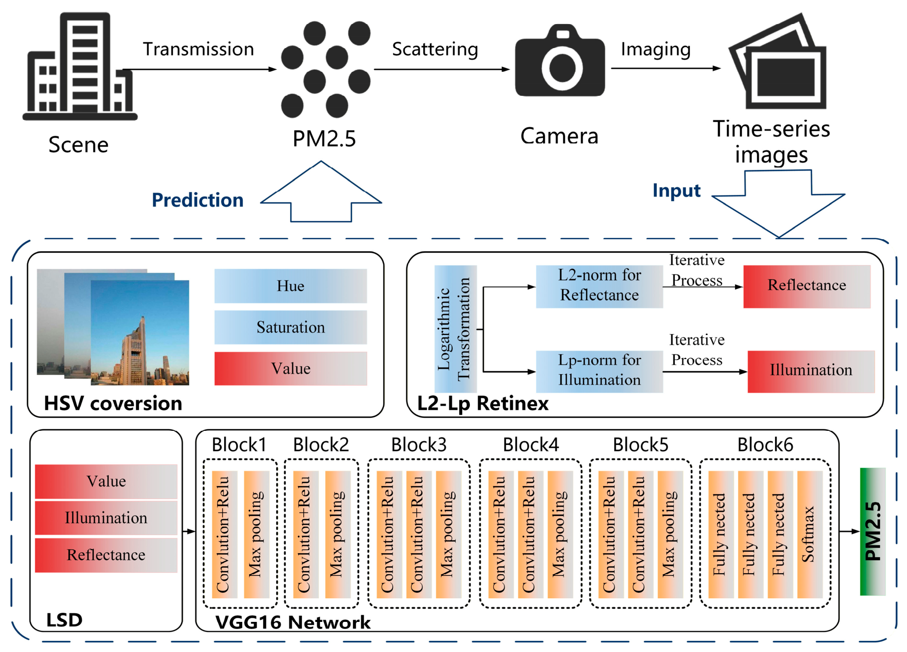The structure of the proposed model is illustrated in Figure 1.

In this study, an LSD module was designed based on Retinex theory and incorporated as a preprocessing component into the VGG16 architecture, resulting in the LSD-CNN model, which enhances the network’s sensitivity to luminance variations. The Retinex algorithm assumes that environmental luminance is determined by two factors: the reflectance component and the illumination component. The corresponding mathematical model is given in Equation (2).

$$I\left(x,y\right)=S\left(x,y\right)\times R\left(x,y\right)$$

(2)

Here, $S(x,y)$ is the illumination component, and $R(x,y)$ is the reflectance component.

Transforming the image into the logarithmic domain not only makes it more consistent with human visual perception but also establishes a connection between the reflectance and illumination components and the target and atmospheric light described, as shown in Equation (3).

$$\mathrm{l}\mathrm{o}\mathrm{g}\left[I\left(x,y\right)\right]=\mathrm{l}\mathrm{o}\mathrm{g}\left[S\right(x,y\left)\right]+\mathrm{l}\mathrm{o}\mathrm{g}\left[R\right(x,y\left)\right]$$

(3)

It can thus be observed that the illumination and reflectance components correspond to the AL and TL in the logarithmic domain, as expressed in Equation (4).

$$\left\{\begin{array}{c}{L}_g=\log \left[S\right(x,y\left)\right]\\ L_t=\log \left[R\right(x,y\left)\right]\end{array}\right.$$

(4)

Therefore, the detailed implementation of the LSD module in this study is as follows:

(1)

To emphasize luminance information, the original image is first converted from the RGB color space to the HSV color space. The luminance component (V) is extracted for LSD.

(2)

The luminance component (V) is then transformed into the logarithmic domain. The L2–Lp variational Retinex algorithm (L2–Lp Retinex) proposed by Fu et al. is applied to decompose the luminance component in the logarithmic domain into illumination and reflectance components [39]. Compared with the conventional Retinex algorithm, the L2–Lp Retinex incorporates an innovative spectrum optimization strategy and a reflectance consistency loss, yielding a more natural and accurate enhancement for low-light images. This makes it particularly suitable for luminance decomposition in PM2.5-affected low-illumination environments.

(3)

Finally, the luminance component (V), illumination component, and reflectance component are combined into a new three-channel image, which is used as the input to VGG16. After being processed by VGG16, a mapping relationship between luminance characteristics and PM2.5 concentration is established.

2.2. Datasets

In this study, long-term publicly available images captured by fixed cameras in Shanghai and Beijing were combined with local PM2.5 monitoring data to construct an image dataset for PM2.5 assessment. The Beijing dataset, constructed by Feng et al., was collected using a fixed camera installed at the Institute of Atmospheric Physics (IAP, Beijing, 116.38°E, 39.97°N, ~10 m elevation), which captured more than 13,000 hourly images [14]. From this dataset, 1952 daytime images taken between 19 May 2019 and 2 March 2020 were selected for analysis. The Shanghai dataset, released by Liu et al., consists of 1954 hourly images of the Lujiazui scene, obtained from the Shanghai Municipal Bureau of Ecology and Environment website [24]. From this dataset, 1648 daytime images taken between 6 May 2014 and 31 December 2014 were selected.

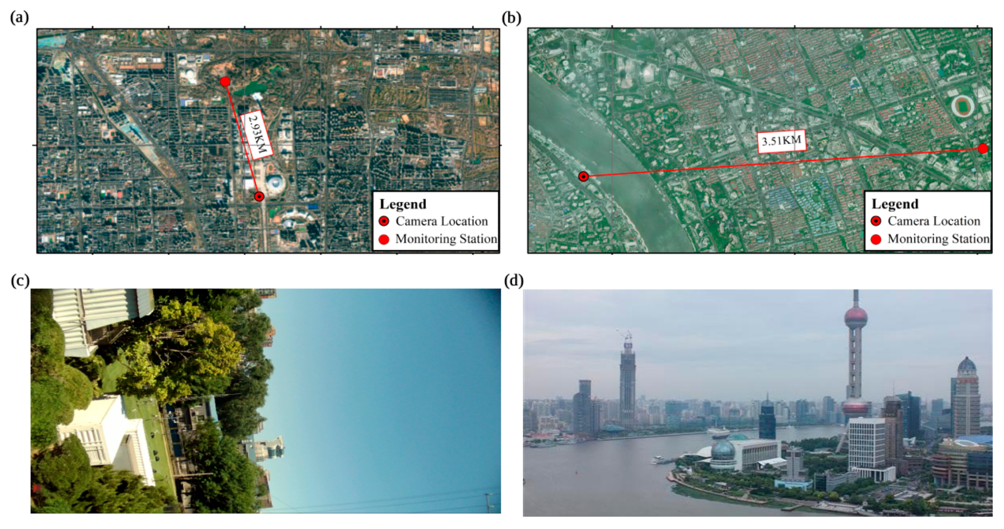
The PM2.5 data corresponding to each image were collected from the historical hourly records published by the China National Environmental Monitoring Center, using the monitoring station nearest to the camera location, as shown in Figure 2. The distances between the two camera sites and their corresponding monitoring stations were less than 4 km, which falls within the spatial representativeness radius specified for urban stations [29]. This validates the use of measurements from the nearest stations as labels for the image dataset.

A small amount of missing data was observed in the annual image and air quality records. To avoid unnecessary errors, images lacking corresponding ground monitoring data were excluded from the dataset. The maximum (Max), minimum (Min), mean (Mean), and standard deviation (Std) of PM2.5 were then calculated for both datasets. The formulas used to compute these metrics are provided in Equations (5)–(8).

$$Max=max\left(x_1,x_1,\dots ,x_n\right)$$

(5)

$$Min=min\left(x_1,x_2,\dots ,x_N\right)$$

(6)

$$Mean={\displaystyle \frac{1}{N}}{\displaystyle \sum _{i=1}^N} x_i$$

(7)

$$Std=\sqrt{{\displaystyle \frac{1}{N}}{\displaystyle \sum _{i=1}^N} {\left(x_i-Mean\right)}^2}$$

(8)

Here, $x$ denotes each PM2.5 label, and $N$ represents the total number of images.

The detailed statistical results are presented in

Table 1. PM2.5 concentration statistics of the two image datasets.

Dataset	PM2.5 (μg/m3)
	Max	Min	Mean	Std
Beijing	262	1	41	41.36
Shanghai	143	16	58	32.93

. In terms of the maximum values, both datasets contain severely polluted cases with high PM2.5 concentrations. Regarding the mean, the overall pollution level in the Shanghai dataset is higher than that in the Beijing dataset, whereas the standard deviation indicates that PM2.5 levels in the Beijing dataset fluctuate more dramatically. In summary, the Shanghai dataset represents a monitoring environment characterized by relatively high but stable pollution levels, while the Beijing dataset corresponds to an environment with a lower overall pollution level but pronounced temporal variability. These two contrasting monitoring environments provide a solid basis for comprehensively evaluating the stability of different image-based PM2.5 estimation methods.

2.3. Model Training

The training was conducted on a server equipped with an Intel(R) Core(TM) i7-14700 CPU (32 GB RAM), an NVIDIA RTX 3500 GPU (43 GB), and Windows 11. The software environment included Python 3.10, PyTorch 2.7, and CUDA 12.8 for GPU acceleration. Standard CNN architectures from PyTorch were employed with a batch size of 16, an initial learning rate of 0.0001, and a training duration of 150 epochs.

Regarding dataset partitioning, this study adopted a stochastic sampling strategy. Given that PM2.5 concentrations typically exhibit a long-tailed distribution where low and moderate pollution levels constitute the majority of observations, a random split is essential to ensure that the training set encompasses a comprehensive range of environmental features and pollution intensities. This approach facilitates the acquisition of robust feature representations and prevents the model from overfitting to specific temporal sequences or chronological trends. In the experimental phase, the dataset was randomly divided into two subsets. The first subset contained 50% of the PM2.5 images, while the second subset contained the remaining 50%. The first subset was used as training data for the regression model, and the remaining 50% was used as test data to evaluate the performance of LSD-CNN and other comparative methods.

To evaluate the generalization performance of the proposed model and address potential concerns regarding data leakage, the RHID-AQI dataset was introduced as a completely independent external benchmark. Performance evaluation on the RHID-AQI dataset was conducted without any retraining or parameter fine-tuning. This cross-dataset validation methodology provides a realistic assessment of the model’s predictive stability in unseen environments and ensures that the results are not biased by temporal correlations within the training data.

2.4. Evaluation Metrics

Three commonly used regression metrics were employed to evaluate the estimation accuracy of the proposed LSD-CNN model: the mean absolute error (MAE), the root mean square error (RMSE) and the Pearson correlation coefficient (PCC).

The mean absolute error (MAE) is defined as

$$MAE={\displaystyle \frac{1}{n}}{\displaystyle \sum _{i=1}^n} \left|y_i-y_i^{\prime }\right|$$

(9)

and the root mean square error (RMSE) is defined as

$$RMSE=\sqrt{{\displaystyle \frac{1}{n}}{\displaystyle \sum _{i=1}^n} {\left(y_i-y_i^{\cdot }\right)}^2}$$

(10)

where $n$ is the number of samples, $y_i$ and $y_i^{\prime }$ are the ith ground truth and the corresponding estimated value, and $\overline{y}$ is the mean of all truth data. When the estimated value is closer to the actual value, the MAE and RMSE are smaller, indicating better model prediction performance.

The Pearson correlation coefficient (PCC) is calculated as

$$PCC={\displaystyle \frac{{\displaystyle {\sum }_{i=1}^n} (y_i-\overline{y})({\widehat{y}}_i-\overline{y})}{\sqrt{{\displaystyle {\sum }_{i=1}^n} (y_i-\overline{y}{)}^2}\sqrt{{\displaystyle {\sum }_{i=1}^n} ({\widehat{y}}_i-\overline{\widehat{y}}{)}^2}}}$$

(11)

where $\overline{y}$ and $\widehat{y}$ are the means of the ground truth and predicted values, respectively. PCC values closer to 1 indicate a stronger linear correlation between predictions and observations.

In summary, smaller MAE and RMSE values and higher PCC values correspond to better model prediction performance.

3. Experimental Results and Analysis

3.1. Effectiveness Verification of LSD

To verify that LSD can partially eliminate the mutual influence between AL and TL—thereby enhancing the independence of luminance information and providing a foundation for subsequent luminance feature extraction—this study conducted a simulation experiment. Specifically, AL and TL images were simulated. The AL image was set to a size of 100 × 100 pixels, with the light source assumed to be located at coordinates (30, 40). The Euclidean distance between each pixel and the light source was computed, and the luminance of each pixel was calculated using a simple inverse-square model, as given in Equation (11).

$$L_{AL}^{sim}\left(x,y\right)={\displaystyle \frac{1}{\left(1+\left(D_{AL}\right(x,y)/\mathrm{m}\mathrm{a}\mathrm{x}(D_{AL}){)}^2\right)}}$$

(12)

Here, $L_{AL}^{\mathrm{s}\mathrm{i}\mathrm{m}}(x,y)$ denotes the simulated luminance of the pixel located at coordinates $(x,y)$, $D_{AL}(x,y)$ represents the distance from this pixel to the light source, and $\mathrm{m}\mathrm{a}\mathrm{x}\left(D_{AL}\right)$ denotes the maximum distance to the light source within the image.

The AL image and the TL image were combined into a simulated image using a weighted fusion approach, where different weights were applied to simulate the effects of atmospheric scattering on luminance information, as expressed in Equation (13). In this study, the weight $\alpha$ was set to 0.5.

$$I^{\mathrm{s}\mathrm{i}\mathrm{m}}=\alpha \cdot L_{\mathrm{s}\mathrm{k}\mathrm{y}}^{\mathrm{s}\mathrm{i}\mathrm{m}}+\left(1-\alpha \right)\cdot L_{\mathrm{t}\mathrm{a}\mathrm{r}}^{\mathrm{s}\mathrm{i}\mathrm{m}}$$

(13)

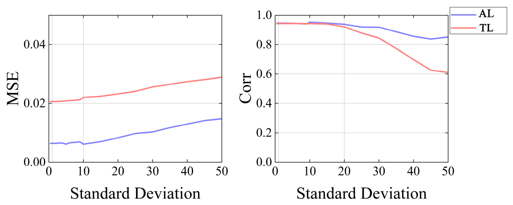
Gaussian filtering was subsequently applied to simulate the decline in visibility caused by variations in PM2.5 concentration. To verify that LSD can effectively reduce the mutual influence between AL and TL, the L2–Lp Retinex was applied to separate the illumination and reflectance components of the simulated images. Correlation coefficients and mean squared errors (MSE) were then computed between these components and the simulated AL and TL images, respectively. As shown in Figure 3, increasing the Std of the Gaussian filter led to higher MSE values and lower correlations between the decomposed AL and TL and their corresponding simulated counterparts. When the Std exceeded 10, the MSE of the decomposition results began to increase significantly but remained below 0.04, indicating a relatively high level of reliability. When the Std exceeded 20, the correlation with the simulated data decreased markedly but still remained above 0.6, suggesting a moderate level of consistency. It should be noted that a relatively large Std was used in the Gaussian filtering process of the simulation experiment to demonstrate the feasibility of the method. In practice, an Std greater than 10 would cause image information to be almost completely lost, making details and edges indistinguishable. Such extreme degradation of image clarity does not occur in real-world scenarios as a result of PM2.5 concentration changes. Therefore, the results demonstrate that the luminance information extracted by the LSD module is reliable.

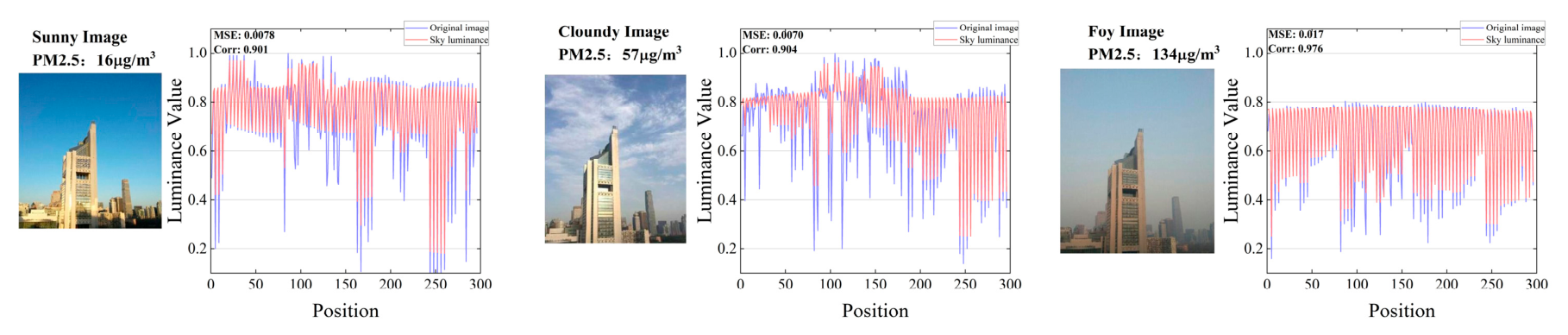
Figure 4 visualizes the separation performance across three distinct scenarios: sunny (PM2.5 = 16 $\mathsf{\mu }\mathrm{g}/{\mathrm{m}}^3$), cloudy (PM2.5 = 57 $\mathsf{\mu }\mathrm{g}/{\mathrm{m}}^3$), and foggy (PM2.5 = 134 $\mathsf{\mu }\mathrm{g}/{\mathrm{m}}^3$). The left column presents the original captures, while the right column provides the one-dimensional luminance intensity profiles, where the original image luminance (blue) and the estimated sky luminance (red) are compared.

As demonstrated in the profiles, the red curve consistently tracks the upper envelope of the blue curve. This alignment indicates that the L2–Lp Retinex successfully extracts the low-frequency AL while effectively filtering out the high-frequency fluctuations caused by the target’s structural details. From a quantitative perspective, the L2–Lp Retinex exhibits high accuracy and robustness even under challenging heavy haze conditions, maintaining a low mean squared error (MSE) of 0.017 and achieving a remarkably high correlation coefficient (Corr) of 0.976. Furthermore, the consistent correlation values exceeding 0.90 across all datasets confirm that the recovered sky luminance is statistically consistent with the original luminance, thereby establishing the L2–Lp Retinex as a reliable physical foundation for the LSD module.

3.2. Quantitative Evaluation of the LSD Module Across Various Network Backbones

In this study, pre-trained VGG16, ResNet50, and MobileNetV2 were adopted as the backbone CNN architectures. By integrating the LSD module into these backbones, this study developed three optimized variants: LSD-VGG16, LSD-ResNet50, and LSD-MobileNetV2. To evaluate the monitoring performance of these models under low-to-moderate pollution conditions, a PM2.5 concentration of 50 $\mathsf{\mu }\mathrm{g}/{\mathrm{m}}^3$ was set as the threshold. Conditions with concentrations below this limit were classified as non-heavily polluted, and all images with PM2.5 levels exceeding 50 $\mathsf{\mu }\mathrm{g}/{\mathrm{m}}^3$ were excluded from the dataset for this specific assessment. The specific results are shown in

Table 2. Quantitative comparison between baseline models and LSD-integrated models under low PM2.5 concentration conditions.

	Shanghai			Beijing
	RMSE	MAE	PCC	RMSE	MAE	PCC
VGG16	7.66	5.83	71.96%	10.49	8.71	62.33%
LSD-VGG16	8.55	6.47	70.24%	10.68	8.86	57.99%
ResNet50	9.54	7.77	52.81%	12.71	10.17	51.81%
LSD-ResNet50	10.78	8.39	49.25%	12.73	10.36	52.48%
MobileNetV2	15.67	12.42	32.10%	19.24	15.47	44.8%
LSD- MobileNetV2	17.77	14.04	35.19%	18.35	14.58	50.33%

.

The experimental results in low PM2.5 scenarios reveal that VGG16 models achieve the most competitive performance, consistently outperforming ResNet50 and MobileNetV2 in terms of error minimization and correlation. Notably, the integration of the LSD module introduces a marginal increase in absolute error under extremely clear conditions. However, it significantly enhances the PCC for backbones with lower feature capacities, such as MobileNetV2. This suggests that the module provides useful physical guidance that complements the limitations of data-driven architectures.

Table 3. Quantitative comparison between baseline models and LSD-integrated models under high PM2.5 concentration conditions.

	Shanghai			Beijing
	RMSE	MAE	PCC	RMSE	MAE	PCC
VGG16	20.37	13.45	84.23%	33.07	24.57	42.11%
LSD-VGG16	19.11	12.42	85.08%	33.07	22.36	45.56%
ResNet50	20.95	13.52	80.56%	34.17	24.49	35.72%
LSD-ResNet50	20.89	13.56	83.50%	33.94	24.17	36.44%
MobileNetV2	22.48	16.72	75.38%	34.49	24.98	25.52%
LSD-MobileNetV2	24.64	17.58	76.08%	33.83	24.57	28.56%

reports the experimental results on the filtered dataset where PM2.5 concentrations exceed 50 $\mathsf{\mu }\mathrm{g}/{\mathrm{m}}^3$, representing heavily polluted or hazy conditions. In stark contrast to the results in low-concentration environments, the integration of the LSD module yields a significant performance improvement across all backbone architectures.

The comparative analysis reveals that VGG16 consistently achieves the highest estimation accuracy and the strongest correlation with ground-truth measurements across both the Shanghai and Beijing datasets. Unlike ResNet50, which utilizes residual connections to capture fine-grained local features, or MobileNetV2, which prioritizes computational efficiency through depth-wise separable convolutions, the hierarchical and sequential structure of VGG16 appears more adept at internalizing the global atmospheric degradation features decoupled by the LSD module. This suggests that for image-based PM2.5 monitoring, where the target signal is often a diffuse, low-frequency atmospheric effect rather than a sharp object-centric feature, the VGG16 backbone offers a more robust network architecture.

This study also identified a universal enhancement in PCC following the integration of the LSD module. As shown in this table, the LSD-integrated models (LSD-VGG16, LSD-ResNet50, and LSD-MobileNetV2) generally achieve lower RMSE and MAE values compared to their vanilla counterparts in most cases. For instance, LSD-VGG16 exhibits a substantial reduction in RMSE on the Shanghai dataset, dropping from 20.37 to 19.11. The PCC values for all backbones increased significantly, with LSD-VGG16 reaching 85.08% in Shanghai and 45.56% in Beijing. This trend clearly indicates that while original CNNs struggle to extract effective features due to the interference of atmospheric light in high PM2.5 scenarios, the LSD module successfully mitigates this issue. The LSD module provides a robust physical constraint that aligns deep learning features with the actual optical reality of atmospheric scattering. Even for MobileNetV2, which inherently possesses limited representation capacity, the LSD module acts as a “physical guide” that compensates for the lack of data-driven feature depth, thereby ensuring that the model captures the correct pollution trends even when absolute numerical errors persist.

Furthermore, the regional disparity observed between the results for Shanghai and Beijing warrants further attention. Across all evaluated scenarios, the error metrics for the Beijing dataset were consistently higher than those for Shanghai, reflecting the inherent environmental complexities and diverse aerosol compositions that characterize different urban landscapes. This performance gap highlights the significant cross-regional transferability challenges faced by purely data-driven deep learning models, a critical issue that is further addressed in Section 4.1. Notably, however, the gain in Pearson correlation coefficient (PCC) afforded by the LSD module was more pronounced in the Beijing dataset. This empirical evidence demonstrates that as environmental conditions become more extreme and purely data-driven features inevitably diminish in reliability, the LSD module provides essential and stable physical priors that anchor the model’s estimation. Consequently, LSD-VGG16 is established as the optimal framework in this study, offering the most robust and balanced performance across varying urban morphologies and pollution intensities.

3.3. Parameter Sensitivity Analysis of the LSD-VGG16

To validate the generalizability and stability of the LSD-VGG16 model, we conducted a sensitivity analysis on a diverse set of hyperparameters. A robust PM2.5 retrieval algorithm should maintain high reproducibility in its convergence behavior under different optimization settings. Accordingly, we analyzed the impact of training parameters on both error metrics and the evolution of loss functions. The Beijing dataset, characterized by its complex urban atmospheric conditions, was utilized as the primary tuning set to facilitate the extraction of high-dimensional image features.

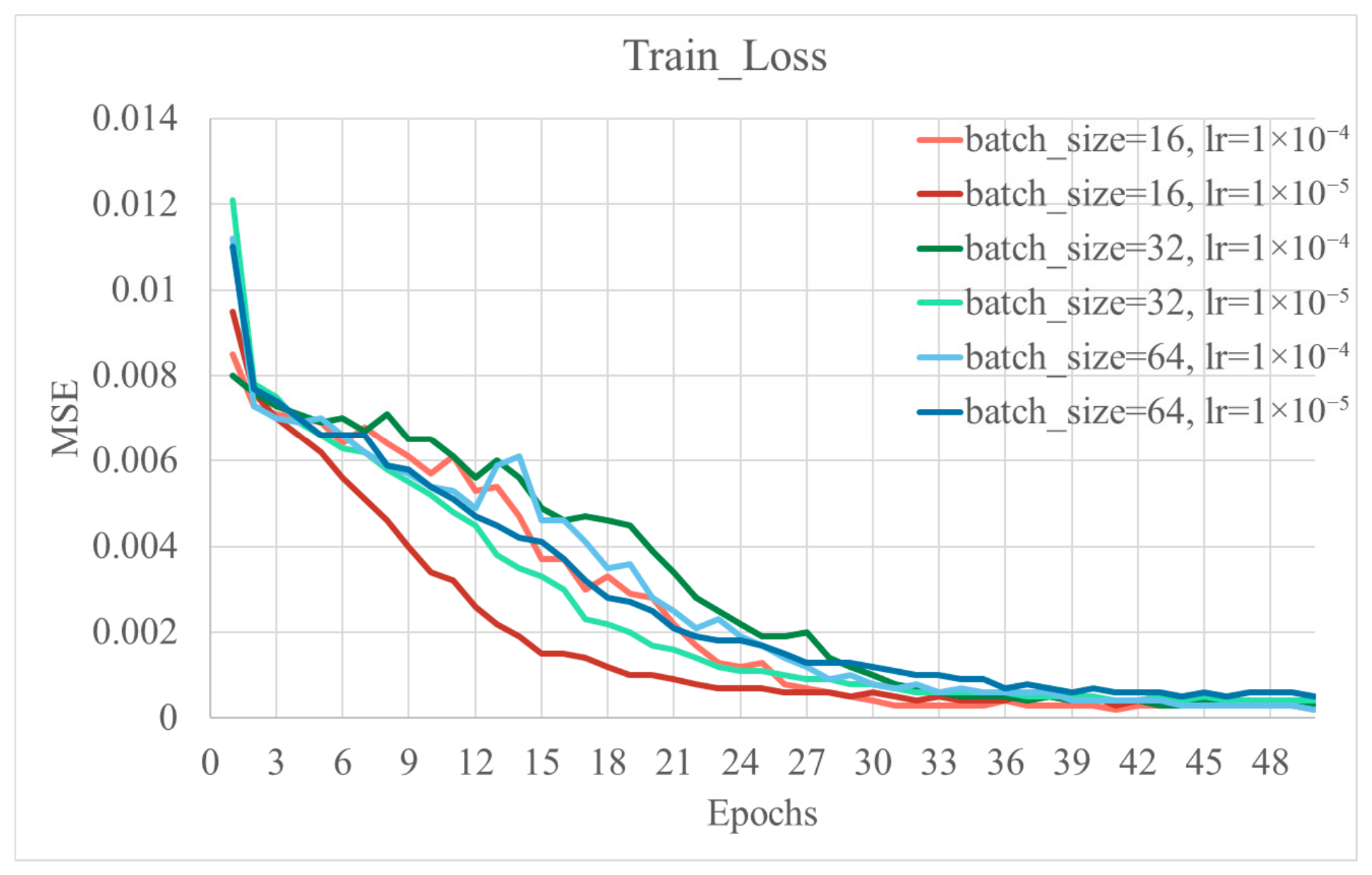
Figure 5 illustrates the evolution of the MSE over 50 training epochs for six distinct hyperparameter configurations. We observe that all tested combinations exhibit a consistent downward trajectory, with the loss values asymptotically approaching a minimum near the end of the 50-epoch cycle. This global convergence behavior demonstrates the inherent stability of the LSD-VGG16 architecture and its capability to effectively minimize the residuals between estimated and ground-truth PM2.5 concentrations within the complex Beijing dataset.

The experimental results indicate that the convergence velocity is significantly influenced by the choice of batch size (BS). Specifically, the configuration with BS = 16 exhibits a more rapid descent in MSE during the initial 20 epochs compared to BS = 32 and BS = 64. This acceleration is primarily attributed to the increased frequency of gradient updates per epoch inherent in smaller batch sizes, which allows the optimizer to navigate the high-dimensional feature space of urban atmospheric images more aggressively. While larger batch sizes (BS = 64) provide more accurate gradient estimates, they often require a higher number of iterations to reach a comparable level of error reduction, as evidenced by their relatively slower initial decay.

Furthermore, the influence of the learning rate (lr) is also critical to the numerical stability of the training process throughout the 50 epochs. A higher lr displays localized stochastic oscillations, particularly for BS = 32 and BS = 64. Such fluctuations suggest that larger step sizes may cause the model to overshoot optimal regions in the loss landscape. In contrast, employing lr = 1 × 10⁻⁴ yields a smoother and more monotonic decline in MSE, facilitating a more stable transition into the final convergence phase.

Ultimately, the combination of BS = 16 and lr = 1 × 10⁻⁵ was identified as the optimal configuration. This setting achieves the most efficient balance between convergence speed and training stability, reaching a stabilized low-loss state earlier than other combinations while maintaining a steady optimization path. Consequently, these parameters were adopted for all subsequent model training and cross-validation procedures to ensure high-fidelity feature representation and robust retrieval performance.

3.4. Attentional Analysis and Performance Evaluation

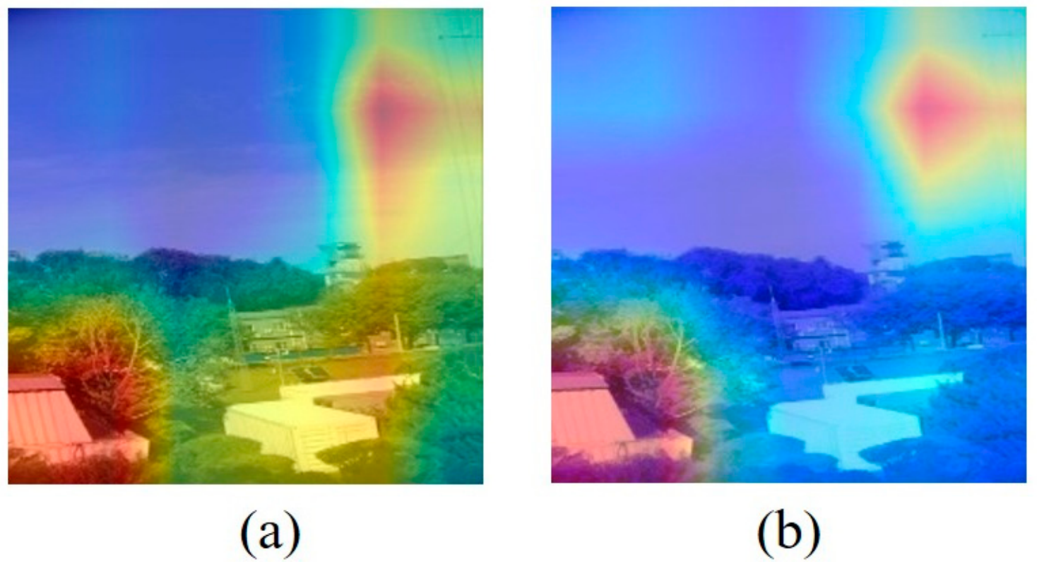
To visually verify the effectiveness of the proposed algorithm, the attention maps of VGG16 and LSD-VGG16 are compared. As illustrated in Figure 6a, the baseline VGG16 exhibits a fragmented attention pattern, predominantly localized on scattered foreground regions. Such over-reliance on complex foreground textures often introduces estimation errors in single-image PM2.5 monitoring tasks. In contrast, the attention regions of LSD-VGG16, shown in Figure 6b, are more focused on the luminance discrepancies between AL and TL.

This divergence in distribution stems from a shift in the feature extraction logic. The VGG16 model relies solely on data-driven texture learning, which is prone to being trapped in sub-optimal local discriminative features. Conversely, LSD-VGG16 integrates the LSD physical prior as a constraint, forcing the network to perceive the physical attributes of illumination during the learning process. This mechanism emulates the perception strategy of the human visual system in complex lighting scenes. Specifically, the ability to adaptively reference AL distribution to calibrate visual representations while focusing on the TL.

The results indicate that LSD guides the neural network to transcend simple statistical correlations toward a deeper understanding of the scene’s physical structure. This not only enhances the discriminative power of the features but also improves their physical adaptability in the absence of sufficiently high pollution images.

Having validated the effectiveness, robustness and physical interpretability of the proposed LSD-VGG16 through comprehensive ablation studies, this study further evaluates its performance against representative methods. Among the three LSD-integrated variants, LSD-VGG16 consistently demonstrates the highest accuracy across both low- and high-PM2.5 concentration scenarios, achieving the lowest RMSE and MAE values in most cases. Consequently, LSD-VGG16 is selected as the baseline for subsequent comparative experiments. The following section presents a detailed quantitative and qualitative comparison between LSD-VGG16 and several mainstream PM2.5 estimation approaches, highlighting the superior performance of our proposed method under diverse atmospheric conditions.

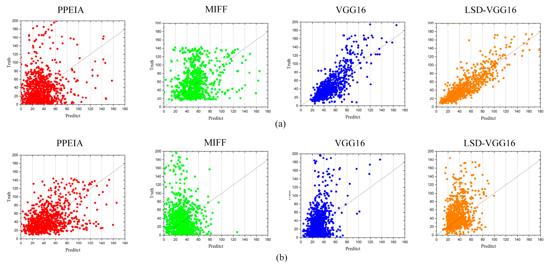
Figure 7 presents scatter plots of predicted versus true PM2.5 concentrations for four methods (PPEIA, MIFF, VGG16, and LSD-VGG16) on the Shanghai and Beijing datasets. The x-axis represents the predicted PM2.5 concentrations, while the y-axis shows the true PM2.5 concentrations. The gray diagonal line indicates the ideal prediction (where predicted values equal true values). The following conclusions can be drawn: (1) The predictions from both PPEIA and MIFF exhibit significant discrepancies from the true values, with the scatter points showing a noticeable divergence along the vertical axis. Particularly under high PM2.5 concentration conditions, the predicted values tend to cluster in the lower range, whereas the true values span a much wider range, indicating a clear underestimation of PM2.5 levels. This suggests that these methods struggle to establish a stable mapping relationship under high PM2.5 concentration conditions, resulting in inaccurate predictions. (2) Compared to PPEIA and MIFF, VGG16 demonstrates a more favorable distribution of scatter points, which are more tightly aligned with the diagonal line. This indicates that deep feature extraction enhances predictive performance to some extent. However, in the Beijing dataset (b), outliers can still be observed in the high-concentration region, with a tendency to underestimate high PM2.5 concentrations. (3) The LSD-VGG16 model stands out as the most accurate in (a), with the scatter points highly concentrated around the diagonal line, indicating a strong linear relationship between predicted and true values. Moreover, in (b), LSD-VGG16 maintains a compact and reliable distribution close to the gray diagonal line, outperforming other methods. These results demonstrate the robustness and reliability of the LSD-VGG16 predictions.

Based on the qualitative analysis of the scatter plots presented in Figure 6, it is clear that while the LSD-VGG16 model outperforms the other representative methods (PPEIA, MIFF, and VGG16) in terms of prediction accuracy and reliability, a more comprehensive evaluation is necessary to quantitatively assess the differences in model performance. Therefore, to further support these observations, this study presents a quantitative performance comparison of all four methods across multiple evaluation metrics, including RMSE and MAE, in

Table 4. Quantitative comparison between representative methods and LSD-VGG16 on the two datasets.

	Shanghai			Beijing
	RMSE	MAE	PCC	RMSE	MAE	PCC
PPEIA	33.70	24.51	67.57%	60.47	41.60	33.51%
MIFF	36.31	26.63	67.65%	48.36	32.49	38.45%
VGG16	20.37	13.45	84.23%	33.07	24.57	42.11%
LSD-VGG16	19.11	12.42	85.08%	33.07	22.36	45.56%

. This table provides a clearer understanding of how each method performs under varying PM2.5 concentrations and highlights the substantial improvements brought by integrating the LSD module into VGG16.

The results in the table indicate that the traditional methods, PPEIA and MIFF, suffer from relatively large prediction errors on both datasets, with a notable increase in RMSE on the Beijing dataset, reflecting their limited robustness under conditions of pronounced temporal variability. In contrast, the deep learning-based VGG16 significantly outperforms these traditional approaches in terms of RMSE and MAE, demonstrating the advantage of convolutional neural networks in extracting discriminative features related to PM2.5 concentrations; however, its performance on the Beijing dataset remains affected by complex pollution patterns and illumination variations. Among all compared methods, LSD-VGG16 consistently achieves the lowest RMSE and MAE, as well as the highest PCC, across both datasets and further reduces the MAE compared with the baseline VGG16, indicating that the incorporation of the LSD module effectively improves prediction consistency and stability. Overall, these quantitative results demonstrate that the proposed LSD-VGG16 achieves superior prediction accuracy and generalization capability across different datasets and pollution conditions, outperforming existing representative methods for PM2.5 estimation.

3.5. Evaluation of Real-World Applicability Across Different Scenes

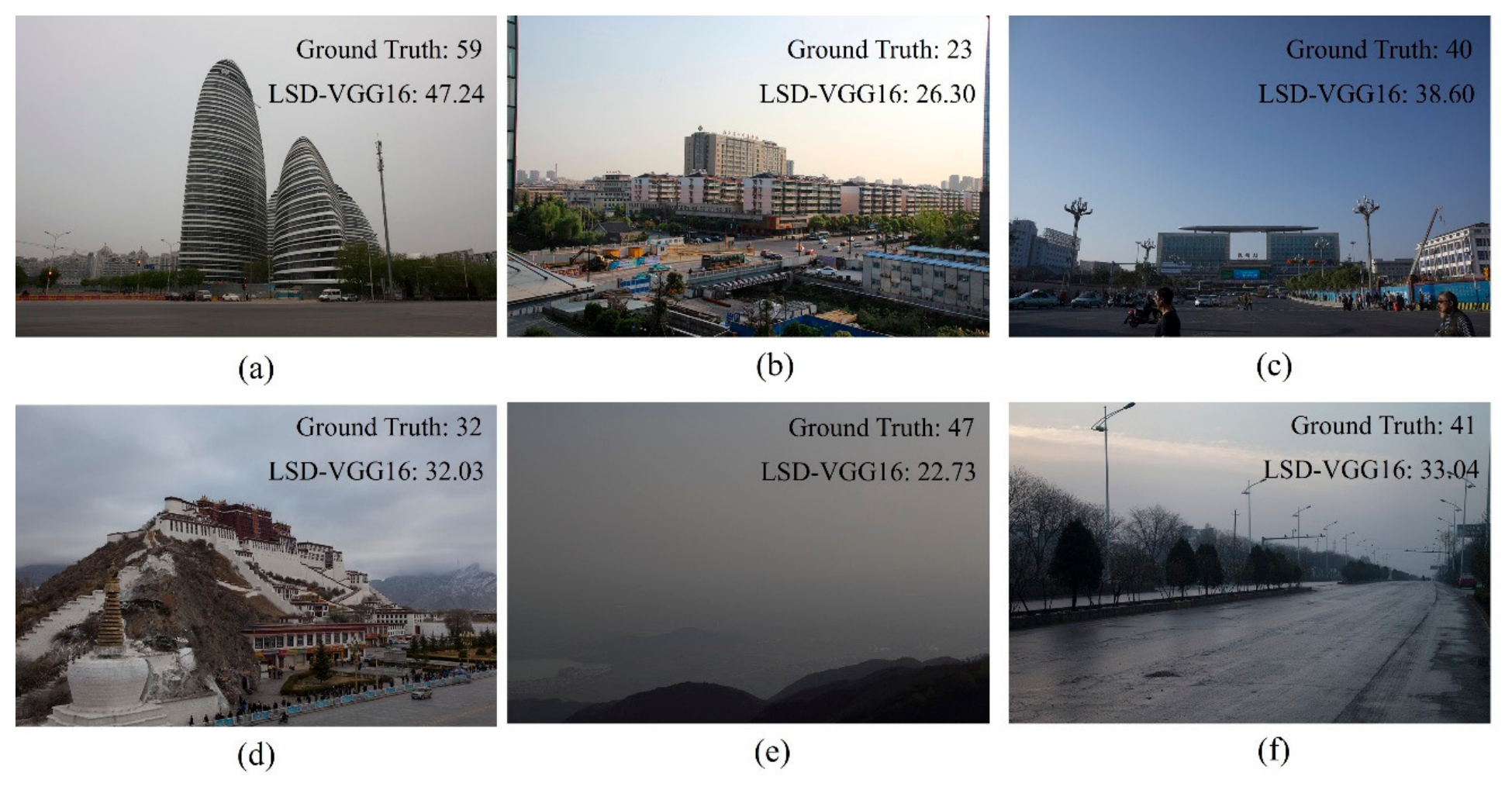
To further validate the robustness and generalization capability of the proposed method, we conducted a qualitative analysis across diverse real-world scenarios. Specifically, this study evaluated the model directly on the RHID-AQI dataset, a new dataset comprising multiple distinct scenes [40,41], without any retraining. As illustrated in Figure 8, the evaluation encompasses diverse scenarios characterized by distinct objects and varying illumination conditions resulting from different weather phenomena, from which three significant observations can be drawn: (1) The proposed method achieves satisfactory accuracy in the majority of cases, highlighting its promising potential to serve as a complementary modality to traditional physicochemical techniques for widespread PM2.5 monitoring. (2) The method exhibits a dependency on distinct targets within the scene to capture feature variations relative to the surroundings; consequently, as evidenced in (e), the absence of clear structural objects leads to a significant deviation of the estimated result from the ground truth. (3) The model demonstrates resilience to abrupt environmental light fluctuations, as shown in (f), where the estimation error remains within a small margin despite marked changes in ambient brightness, confirming its robustness against illumination variability.

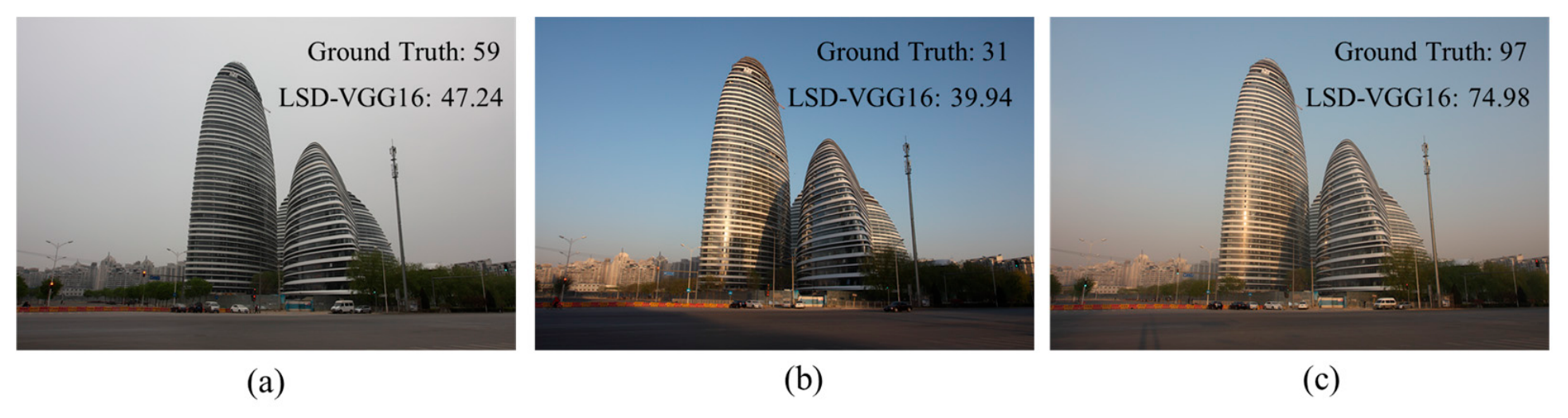
As shown in Figure 9, the proposed LSD-VGG16 model is evaluated across different weather conditions within the same urban environment (Beijing). Under cloudy and polluted conditions, as shown in Figure 9a, the model produces a prediction of 47.24$\mathsf{\mu }\mathrm{g}/{\mathrm{m}}^3$^, relatively close to the ground truth of 59 $\mathsf{\mu }\mathrm{g}/{\mathrm{m}}^3$. In the sunny and clean scenario, as shown in Figure 9b, the predicted value of 39.94 $\mathsf{\mu }\mathrm{g}/{\mathrm{m}}^3$ slightly overestimates the ground truth of 31 $\mathsf{\mu }\mathrm{g}/{\mathrm{m}}^3$. In contrast, under sunny yet polluted conditions, as shown in Figure 9c, the model yields a prediction of 74.98 $\mathsf{\mu }\mathrm{g}/{\mathrm{m}}^3$ that underestimates the true value of 97 $\mathsf{\mu }\mathrm{g}/{\mathrm{m}}^3$, with a relatively larger deviation compared to the other cases.

This performance variation reflects the intrinsic difficulty of single-image PM2.5 estimation under different weather conditions. When the environment is relatively homogeneous, as shown in Figure 9a,b, the overall estimation accuracy is reliable. However, as shown in Figure 9c, when the environment is affected by both a strong light source, such as the sun, and high levels of PM2.5 pollution, the results show significant deviations. If the model relied only on deep learning to learn image-texture features at this stage, serious misclassifications could occur. However, the incorporation of LSD helps the model capture physically meaningful properties of the environment, enabling it to reconstruct the approximate level of air pollution as accurately as possible.

Overall, these results demonstrate that the proposed LSD-VGG16 achieves robust cross-scenario performance within a unified urban setting, effectively adapting to variations in weather and pollution conditions. Although slight biases exist under extreme conditions, the integration of the LSD physical prior significantly enhances the model’s ability to extract physically meaningful features, leading to improved generalization, stability, and interpretability in real-world PM2.5 estimation tasks.

4. Discussion

4.1. Cross-Scene Performance Disparities and Physical Prior

Experimental results demonstrate that environmental variations inevitably lead to fluctuations in model performance, particularly in the high-pollution image samples within the Beijing dataset. It is crucial to clarify that such accuracy degradation is not an inherent flaw of the LSD module, but rather a universal challenge in the field of image-based PM2.5 monitoring, because this method relies on a single image, and there are not enough training samples with high PM2.5 concentrations. Deep learning models are inherently dependent on data distribution; when image features of extreme pollution episodes are underrepresented in the training set, standard convolutional neural networks (CNNs) struggle to capture complex nonlinear mapping relationships.

To address this issue, the LSD module is specifically designed to introduce prior physical constraints by mimicking the physical principles of human visual perception. By decoupling the original image into AL and TL, the LSD module explicitly enhances the physical representation of image degradation caused by haze. This mechanism helps improve the stability of the model in extreme environments, even in the absence of sufficient high-pollution training data. This underscores the superiority of physics-inspired modules in alleviating the data imbalance problem. Future endeavors should focus on constructing comprehensive, multi-dimensional datasets with broader spatial-temporal spans and more extreme pollution scenarios to further push the accuracy boundaries of deep learning models in PM2.5 estimation tasks.

4.2. Impact of Temporal Span and Static Feature Representation

The datasets employed in this study span from 2014 to 2020. It is well-acknowledged that for continuous time-series monitoring, which requires capturing dynamic evolutionary patterns, a broad temporal span can negatively affect deep learning models due to shifts in atmospheric composition and climatic backgrounds. However, the methodology proposed in this work fundamentally relies on PM2.5 estimation from a single image per day.

Under this static image-based monitoring paradigm, the extended time span does not compromise model stability. Instead, it serves as a mechanism for feature enrichment. By incorporating diverse aerosol distributions, varying illumination conditions, and heterogeneous background noise from different years, the model’s capacity to capture spatial structural features is enhanced, thereby broadening its generalization boundaries across diverse atmospheric environments. The experimental results demonstrate that LSD-VGG16 can extract robust physical features from temporally heterogeneous samples. It should be noted that if future research shifts toward intra-day continuous real-time monitoring, incorporating temporal continuity modeling will be essential to capture the dynamic diffusion of pollutants.

5. Conclusions

In general, image-based PM2.5 monitoring holds significant promise as a complementary approach to traditional monitoring techniques. However, achieving precise predictions in severely polluted environments characterized by extremely high PM2.5 concentrations remains a challenge, as existing deep learning methods often suffer from substantial estimation errors. This study investigates the complex relationship between image luminance and PM2.5 concentrations to enhance the accuracy of image-based monitoring and proposes an LSD module constructed based on L2–Lp Retinex theory. The key conclusions are summarized as follows:

(1)

Simulation experiments validated the reliability of the L2–Lp Retinex-based decomposition method. Quantitative results demonstrate that the luminance component separated by the algorithm exhibits minimal error compared to the simulated ground truth. This high-fidelity extraction provides a solid physical foundation for the subsequent construction of the LSD module, ensuring the accurate separation of AL and TL to facilitate downstream feature extraction.

(2)

Ablation studies confirmed that the LSD module effectively resolves the conflict between mitigating high-concentration haze interference and preserving image features. The module exhibits an adaptive gain characteristic: in low-pollution scenarios, it introduces low interference to the backbone network, thereby maintaining baseline accuracy. Conversely, in high-pollution conditions, it acts as a critical correction model, significantly reducing prediction errors. This dual characteristic ensures the model’s resilience to atmospheric degradation without compromising performance under clear weather conditions, validating its robustness as an all-weather PM2.5 estimation solution.

(3)

Comparative experiments demonstrate that the proposed LSD-VGG16 significantly outperforms traditional methods (PPEIA and MIFF) and standard deep learning approaches (VGG16). While traditional methods struggle to cope with drastic temporal variations in PM2.5 concentrations and standard CNNs remain susceptible to interference in high-concentration environments, LSD-VGG16 consistently achieves the lowest errors across almost all datasets. This confirms that the integration of the LSD module enhances luminance feature discriminability and model stability, establishing the framework as a highly effective and generalizable solution.

(4)

The generalization capability of the model was evaluated on the real-world, multi-scenario RHID-AQI dataset. Without any retraining, LSD-VGG16 leveraged pre-trained parameters to demonstrate adaptability to abrupt illumination fluctuations and diverse weather conditions. This indicates its potential to serve as a significant complementary technology to traditional physicochemical monitoring techniques.

It is worth noting that the proposed method relies on structural cues for optimal feature extraction, and performance may degrade in scenes lacking distinct targets. Despite this specific limitation, the method’s overall stability in dynamic environments provides valuable insights and serves as a reference for future research and applications.