Monitoring Abandoned Cropland in Fragmented Mountainous Landscapes Based on the ML-LandTrendr Framework

Highlights

What are the main findings?

• A ML-LandTrendr framework was developed to map abandoned cropland in hilly and mountainous terrain.
• DtT, GTO, and GDP are identified as the major driving factors of cropland abandonment.
• Through quantitative analyses, the major driving factors of cropland abandonment were identified, the contribution of each factor was quantified, and key interactive effects were highlighted.

What are the implications of the main findings?

• This study provides a replicable technical framework integrating “change detection, machine learning, and nonlinear driving force analysis” for the upper Yangtze River region and similar hilly areas.
• The findings will directly inform regional cropland protection policy formulation, sustainable agricultural management, and the construction of ecological security barriers in the Yangtze River Basin.

Abstract

Cropland abandonment is increasing in the upper and middle Yangtze River Basin due to complex terrain, urbanization, and labor migration. This threatens regional food security. To address the challenge of monitoring abandonment in fragmented hilly areas, we developed a framework. We integrated machine learning with time-series analysis. We mapped cropland probability using multi-source remote sensing data, random forest, and kernel density estimation, then applied LandTrendr to detect land-use changes and track the spatiotemporal evolution of abandonment from 2000 to 2022. Next, we combined Geodetector and linear regression to identify driving factors. The results show that abandoned cropland exhibited an increasing trend from 2000 to 2010, with an average annual growth rate of 20.4%. From 2010 to 2013, the area of abandoned cropland declined rapidly, decreasing by 44.6%. Between 2013 and 2022, abandoned cropland decreased steadily, with an average annual reduction rate of 24.7%. Spatially, abandonment was clustered in the central mountains and southern hills. Key drivers included distance to towns (DtT), total grain output (GTO), and GDP. Our approach supports cropland management and rural revitalization in regions with complex terrain.

1. Introduction

Cropland is vital for food security and sustainable development [1,2,3]. Despite China’s strict protection policies, cropland abandonment remains widespread [4]. This trend is driven by urbanization and socio-economic shifts, particularly in mountainous regions [2]. Abandonment significantly impacts both the environment and society [5]. On one hand, it can enhance soil stability, strengthen carbon sequestration, improve water and nutrient cycles [6], and promote ecosystem restoration. On the other hand, it may lead to reduced grain yields [7] and threaten traditional agricultural landscapes and biodiversity [8]. Consequently, it undermines food security and causes socio-economic instability.

Accurate monitoring of long-term cropland abandonment is fundamental to understanding its spatiotemporal dynamics. In hilly and mountainous areas, traditional field surveys (e.g., household questionnaires, plot sampling) are accurate but inefficient, costly, and unsuitable for large-scale, periodic monitoring. Remote sensing has become a mainstream tool for mapping abandoned cropland because it enables rapid, wide-area, and repeatable observations [9,10,11]. Recent advances in cloud computing platforms (e.g., Google Earth Engine) have removed barriers to data processing and storage [12,13,14,15], supporting long-term dynamic monitoring of abandonment. Existing remote sensing methods for detecting abandoned cropland fall into three categories: (1) time-series change detection based on vegetation indices (e.g., thresholding or differencing of NDVI/EVI to identify spectral declines from cultivation to abandonment) [15,16]; (2) single- or multi-date supervised classification (e.g., random forest, support vector machines) that directly classifies cropland and non-cropland, but often misclassifies abandoned cropland as grassland or bare soil [17]; and (3) post-classification change detection, which classifies each date separately and then compares class changes to identify abandonment. This approach suffers from accumulated classification errors [18]. Despite many studies, two key challenges remain in monitoring long-term abandonment in hilly regions: (i) inter-annual spectral fluctuations (due to climate and phenology) causing false changes, and (ii) spectral confusion between cropland, grassland, and bare soil, which cannot be resolved by single-date classification or simple differencing. Thus, a robust method is needed that captures long-term trends, suppresses inter-annual noise, and does not rely on a single spectral feature.

LandTrendr (Landsat-based Detection of Trends in Disturbance and Recovery) is a temporal segmentation algorithm for time-series spectral trajectories [18,19]. It fits piecewise linear lines to per-pixel annual time series (e.g., spectral bands, vegetation indices) and identifies breakpoints, thereby quantifying the year, magnitude, and recovery rate of disturbance events (e.g., deforestation, urbanization, and abandonment). In land-use change research, LandTrendr serves a clear role: it is a long-term, trend-driven disturbance detection method, not a simple two-date comparison. Its advantages include: (1) long-term trend-fitting that reduces false changes from inter-annual climate variability, outperforming two-date differencing; (2) simultaneous extraction of change magnitude and duration, allowing distinction between short-term fallow and long-term abandonment; and (3) strong compatibility with historical Landsat archives (TM/ETM+/OLI), suitable for time-series analysis since 2000. LandTrendr [18] has been widely used in forest disturbances, fire scars, and urban expansions, but less so in cropland abandonment mapping. A few studies applied LandTrendr directly to vegetation index time series (e.g., NDVI, EVI) to identify persistent spectral decline as abandonment [18,19]. However, this still relies on a single spectral index and cannot fundamentally solve the misclassification of grassland and bare soil, nor does it capture the spatial continuity of cropland. To overcome these limitations, we propose a new framework for extracting abandoned cropland. First, we apply an annual multi-feature random forest classification, combining spectral, textural, topographic, and tasseled cap transformation features to produce annual cropland/non-cropland binary maps. Random forest handles high-dimensional nonlinear relationships and resists overfitting, reducing single-date misclassification. Second, we perform kernel density estimation to generate cropland probability maps, converting discrete binary pixels into a continuous probability surface. Each pixel’s probability represents cropland density in its neighborhood, reflecting spatial continuity and smoothing local classification noise. Third, we feed the annual cropland probability time series (not raw spectral or vegetation index data) into LandTrendr to fit probability trajectories. When a pixel shows a significant and sustained decline in cropland probability (from high to low), it is identified as abandonment. The innovation lies in extending LandTrendr’s application from spectral features to cropland probability. Probability values more directly indicate “cropland likelihood” and are less affected by inter-annual phenological fluctuations. Meanwhile, kernel density introduces spatial context, greatly improving robustness to mixed pixels and grassland confusion.

Identifying the drivers of cropland abandonment is essential for designing targeted protection policies. Previous studies often used linear regression or logistic regression to relate a single or a few factors (e.g., slope, elevation, and labor migration) to abandonment probability [8,18,19,20,21,22,23,24,25,26,27,28,29,30]. Abandonment results from complex interactions among natural (e.g., topography), socio-economic (e.g., labor migration), and locational (e.g., distance to towns) factors [18]. In hilly regions with rugged terrain, nonlinear interactions are common—for example, steep slopes combined with proximity to forest margins produce much higher abandonment rates than the sum of individual effects. Traditional linear methods struggle to capture the nonlinear mechanisms behind such spatial heterogeneity [31,32]. The Geodetector is a spatial variance-based statistical tool designed to detect spatial differentiation and its drivers [33]. Its strengths are: (1) it does not assume linearity and can detect any type (including nonlinear) of causal relationship; and (2) it quantifies interaction effects between two factors, e.g., whether slope and distance to roads together exert a stronger influence on abandonment than the sum of their individual effects (i.e., two-factor enhancement). Thus, Geodetector provides a powerful way to understand the complex human–land relationships behind abandonment. It has been widely used in land-use change and environmental health, but rarely in analyzing abandonment drivers in hilly areas.

This study aims to reveal the long-term spatiotemporal patterns and multi-factor driving mechanisms of cropland abandonment in the upper reaches of the Yangtze River, using Luzhou City, Sichuan Province, as a case study. Luzhou is characterized by low mountains, hills, and valley plains—a typical “mountain–hill–basin” landscape. In recent years, this region has experienced sharp conflicts among urbanization, rural labor outmigration, and cropland protection, with increasingly prominent abandonment, making it a representative case. We address two questions:

(1)

What were the spatiotemporal patterns (abandoned area, spatial distribution, hotspots, and duration) of cropland abandonment in Luzhou from 2000 to 2022?

(2)

How do natural, socio-economic, and locational factors drive the abandonment process? Which factors dominate, and do they show interaction enhancement?

To answer these questions, we first extract annual abandoned cropland information using Landsat time series (2000–2022) coupled with LandTrendr, a multi-feature random forest model, and kernel density analysis. Second, we use spatial statistics (global and local Moran’s I) to analyze clustering patterns of abandonment. Third, we quantify the contribution of each driver and their interactions using Geodetector (factor and interaction detection) combined with linear regression models.

2. Materials and Methods

2.1. Study Area

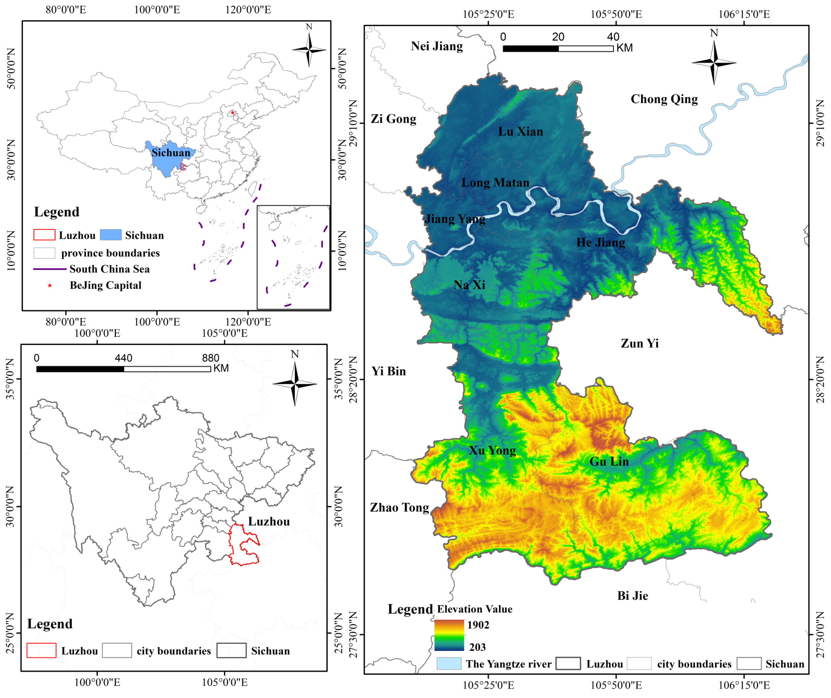
Luzhou City is located in southeastern Sichuan Province, in the upper and middle Yangtze River Basin (27°39′–29°20′N, 105°8′–106°28′E). It covers 12,236.2 km² and administers three districts and four counties (Figure 1). The terrain consists mainly of low and medium mountains. The elevation ranges from 203 m in the central Yangtze River valley to 1902 m in the south, forming a “saddle-like” topography. This rugged and fragmented terrain results in small, scattered cropland plots. These conditions hinder mechanization and increase the risk of abandonment. The region has a subtropical humid climate with an annual precipitation of 1016.2 mm. While the warm and wet conditions support crops, frequent cloud and fog cover make it difficult to acquire high-quality optical remote sensing imagery.

2.2. Data Sources and Preprocessing

2.2.1. Landsat Imagery Processing

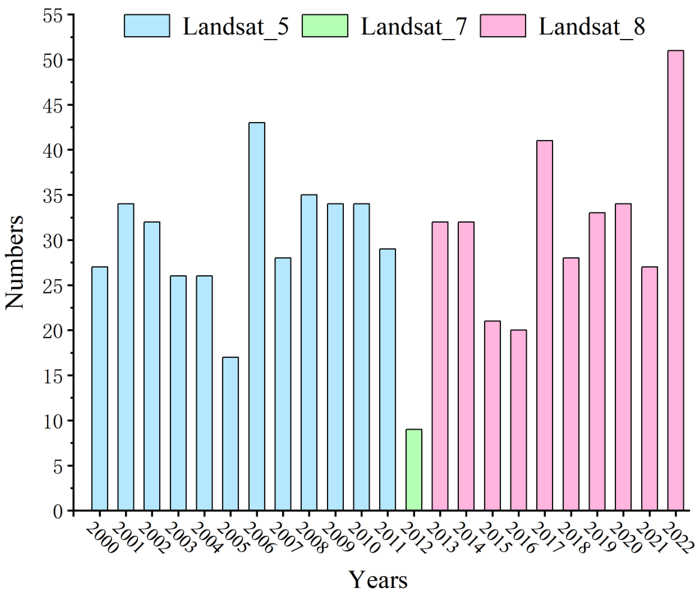
The growing season in the Yangtze River Basin extends from March to October. Therefore, we selected Landsat images from this period [34]. Due to frequent clouds, we prioritized images with less than 10% cloud cover. We also included images with up to 20% cloud cover to ensure sufficient data. This resulted in a total of 693 scenes. Furthermore, we mapped the spatial distribution and calculated the number of available pixels each year in the study area (Figure 2). To clean the data, we used Quality Assessment (QA) bands to mask clouds and shadows. For Landsat 7 ETM+ images, we repaired the scan line gaps using linear interpolation. Finally, we created median composites and cropped them to the study area. Detailed band parameters of the Landsat 5, Landsat 7, and Landsat 8 images are presented in

Table 1. Band parameters of Landsat 5, Landsat 7, and Landsat 8 images.

Sensor	Main Band	Band Name	Wavelength (μm)	Spatial Resolution
Landsat 5 TM/7 ETM+	Band1	Blue	0.45–0.52	30 m
	Band2	Green	0.52–0.60	30 m
	Band3	Red	0.63–0.69	30 m
	Band4	Near-Infrared (NIR)	0.76–0.90	30 m
	Band5	Shortwave Infrared 1 (SWIR1)	1.55–1.75	30 m
	Band7	Shortwave Infrared 2 (SWIR2)	2.08–2.35	30 m
Landsat 8 OLI	Band2	Blue	0.45–0.51	30 m
	Band3	Green	0.53–0.59	30 m
	Band4	Red	0.64–0.67	30 m
	Band5	Near-Infrared (NIR)	0.85–0.88	30 m
	Band6	Shortwave Infrared 1 (SWIR1)	1.57–1.65	30 m
	Band7	Shortwave Infrared 2 (SWIR2)	2.11–2.29	30 m

.

2.2.2. Other Data

This study also incorporated topographic, socio-economic, and foundational geospatial data. Topographic data were derived from a 30 m-resolution Digital Elevation Model (DEM) from 2009 to 2020, sourced from the Geospatial Data Cloud platform. These data were used to extract key natural factors such as elevation and slope. Socio-economic data, covering the period from 2000 to 2022, included metrics such as Gross Domestic Product (GDP), employment in the primary industry, total grain output, and rural population. These statistics, obtained from the Resource and Environmental Science and Data Center, were used to quantify the socio-economic drivers of cropland abandonment. Furthermore, to construct a comprehensive set of explanatory variables and support high-accuracy validation, the study acquired road network and river vector data from 2000 to 2020, as well as GF-2 high-resolution imagery and data on cropland gain and loss from 2015 to 2022. These additional datasets were sourced from the Resource and Environmental Science and Data Center and the China Platform of Earth Observation System. Please refer to

Table 2. Data source table.

Name	Time	Data Type and Resolution	Source
Land-Use Data	2000–2020	TIFF	https://www.resdc.cn/Default.aspx/ (accessed on 2 January 2025)
DEM	2009–2020	TIFF	https://www.gscloud.cn/ (accessed on 2 January 2025)
Statistical Yearbook Data	2000–2022	CSV	https://www.resdc.cn/Default.aspx/ (accessed on 2 January 2025)
Road and River Network Data	2020	SHP	https://www.resdc.cn/Default.aspx/ (accessed on 2 January 2025)
GF-2	2015–2022	TIFF	https://www.cpeos.org.cn/research/#/ (accessed on 2 January 2025)
Google Earth	2000–2022	TIFF	https://earth.google.com/ (accessed on 2 January 2025)
Image Data	2000–2022	TIFF	https://www.resdc.cn/Default.aspx/ (accessed on 2 January 2025)
Administrative Boundary Data	2022	SHP	http://www.resdc.cn/DOI (accessed on 2 January 2025)
Cultivated Land Gain–Loss Data and National Land Survey Data	2010–2023	SHP	Sichuan Provincial Department of Natural Resources

for the details of all data sources.

2.3. Methods

2.3.1. Generation of Annual Cropland Probability Maps

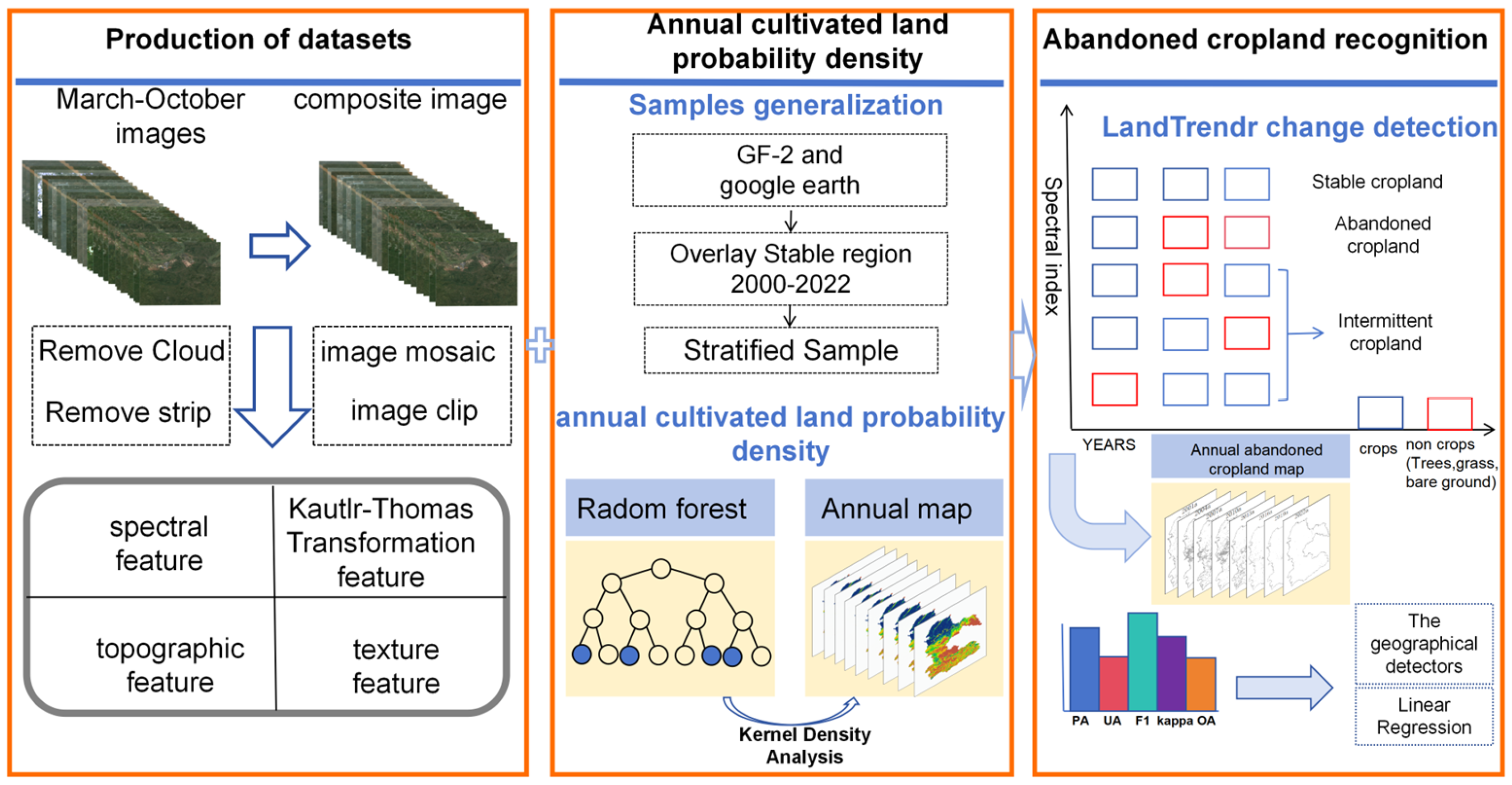
To obtain accurate maps of abandoned cropland, identify the spatiotemporal characteristics of its distribution, and to clarify the driving factors influencing its changes, a systematic technical workflow was adopted in this study, consisting of three key steps as follows: First, high-precision cropland probability maps were generated. Based on Landsat 5/7/8 imagery, a comprehensive set of feature factors was extracted, including spectral, textural, tasseled cap transformation, and topographic features. Subsequently, the random forest model and kernel density analysis method were employed to map the spatial distribution of cropland probability. Second, the LandTrendr change detection algorithm was applied to identify and analyze the inter-annual variations in cropland probability, thereby accurately determining the spatial distribution of abandoned cropland. Finally, the distribution characteristics of abandoned cropland were analyzed in combination with 14 potential influencing factors to identify the primary driving factors affecting its occurrence and spatial pattern. The specific technical workflow comprises three core steps: generation of annual cropland probability maps, cropland abandonment identification and mapping, and determination of major driving factors (including Geodetector and linear regression analysis). The technical workflow diagram is presented in Figure 3.

We derived features from Landsat imagery, including spectral, textural, tasseled cap transformation (a graphic description of the spectral–temporal development of agricultural crops as seen by Landsat) [34], and topographic data. We then produced a cropland probability map for 2000–2022 using a random forest (RF) [35] classifier and kernel density analysis. Using six Landsat bands, we calculated the Normalized Difference Vegetation Index (NDVI), Enhanced Vegetation Index (EVI), and Normalized Difference Water Index (NDWI). To capture seasonal variations, we generated 20th- and 80th-percentile composites for each year. The formulas are as follows:

$$NDVI={\displaystyle \frac{{\rho }_{NIR}-{\rho }_{RED}}{{\rho }_{NIR}+{\rho }_{RED}}}$$

(1)

$$EVI=2.5\cdot \left({\displaystyle \frac{{\rho }_{NIR}-{\rho }_{RED}}{{\rho }_{NIR}+6·{\rho }_{RED}-7.5·{\rho }_{BLUE}+1}}\right)$$

(2)

$$NDWI={\displaystyle \frac{{\rho }_{GREEN}-{\rho }_{NIR}}{{\rho }_{GREEN}+{\rho }_{NIR}}}$$

(3)

where ${\rho }_{RED}$, ${\rho }_{NIR}$, ${\rho }_{BLUE}$, and ${\rho }_{GREEN}$ represent the reflectance of the red, near-infrared, blue, and green bands, respectively.

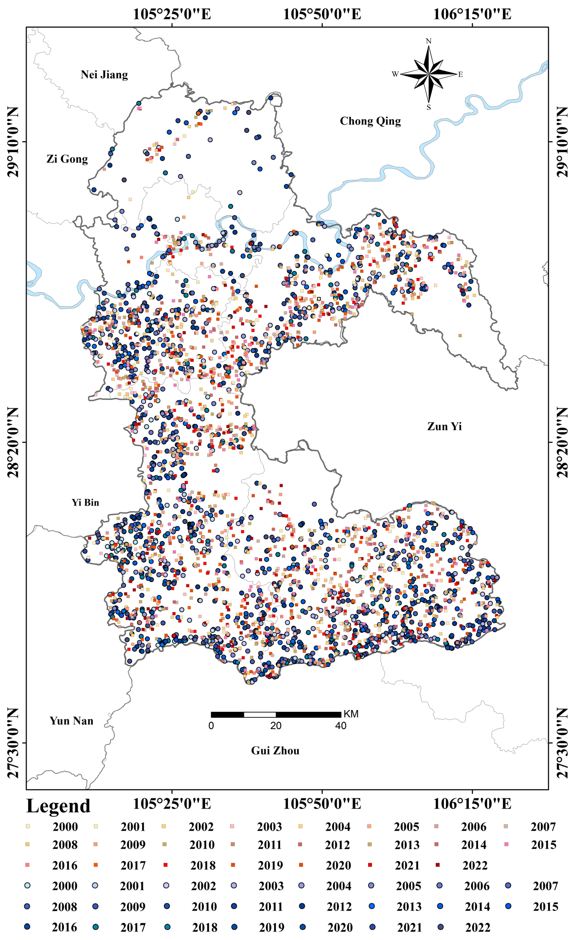
We applied the tasseled cap transformation to derive Brightness (TCB), Greenness (TCG), and Wetness (TCW). These components help distinguish bare soil, vegetation, and moisture. We also calculated textural features (Contrast, Variance, and Mean) using the Gray-Level Co-occurrence Matrix (GLCM). Combined with topographic factors, the final feature set included 23 variables, refer to

Table 3. Variable indicators.

Categories	Number	Feature Name	Abbreviation
Original Landsat Spectral Bands	1	Blue band reflectance	Blue
	2	Green band reflectance	Green
	3	Red band reflectance	Red
	4	Near-infrared band reflectance	NIR
	5	Shortwave infrared 1 reflectance	SWIR1
	6	Shortwave infrared 2 reflectance	SWIR2
Spectral Vegetation Index	7	Normalized Difference Vegetation Index	NDVI
	8	Enhanced Vegetation Index	EVI
	9	Normalized Difference Water Index	NDWI
Percentile Vegetation Index	10	20th-percentile Normalized Difference Vegetation Index	NDVI_p20
	11	80th-percentile Normalized Difference Vegetation Index	NDVI_p80
	12	20th-percentile Enhanced Vegetation Index	EVI_p20
	13	80th-percentile Enhanced Vegetation Index	EVI_p80
	14	20th-percentile Normalized Difference Water Index	NDWI_p20
	15	80th-percentile Normalized Difference Water Index	NDWI_p80
Tasseled Cap Transformation	16	Tasseled Cap Brightness	TCB
	17	Tasseled Cap Greenness	TCG
	18	Tasseled Cap Wetness	TCW
GLCM Textural Features	19	Angular second moment	ASM
	20	Contrast	Contrast
	21	Variance	VAR
Topographic Factors	22	Slope	Slope
	23	Elevation	Elevation

for specific variable indicators. To ensure classification accuracy, we collected training samples via visual interpretation of high-resolution images (Google Earth and GF-2). The samples were split into independent training and test sets at a ratio of 7:3. This resulted in 1764 cropland samples and 1641 other samples (representing all land cover types except cropland) for the period 2000–2022. The annual distribution of these samples is shown in Figure 4. For the random forest algorithm, the training set and test set followed a 7:3 ratio.

We generated annual land cover maps using the random forest (RF) algorithm. While RF provides class probabilities, these probabilities are pixel-wise and often exhibit spatial discontinuities (i.e., salt-and-pepper noise), which can be problematic for subsequent change detection [36]. To address this, following previous studies, we applied kernel density estimation (KDE) to convert the binary classification into a continuous probability surface [37]. Unlike raw RF probabilities, KDE explicitly incorporates local spatial context, aggregates neighboring pixel information, and reduces isolated misclassifications while preserving overall cropland parcel shapes. This smoothed probability map serves as a more robust input for the LandTrendr algorithm, improving its ability to detect genuine land-use changes by suppressing transient noise. Detailed parameters for both RF classification and KDE are provided in

Table 4. Parameter information related to random forest and kernel density analysis.

Method	Parameter Name	Parameter Value
Random forest	numberOfTrees	150
	variablesPerSplit	5
	minLeafPopulation	3
	bagFraction	0.7
	maxNodes	null
	Seed	42
Kernel density	Kernel function type	Gaussian kernel
	Fixed bandwidth	300 m

.

2.3.2. Cropland Abandonment Identification and Mapping

To distinguish abandonment from crop rotation or short-term fallow, we established specific rules based on local practices. Following previous studies [12,22,36,37,38,39,40], we defined “abandoned cropland” as parcels cultivated in the starting year that showed a sustained probability decline for two or more consecutive years. We excluded short-term fallow to avoid confusion. Specifically, parcels showing a “cultivation–pause–cultivation” pattern within three years were removed. Finally, we accounted for the “Grain for Green” policy. Parcels on slopes steeper than 25° that transitioned to forest or grassland were classified as ecological restoration, not spontaneous abandonment.

We used the LandTrendr algorithm to detect changes in the cropland probability time series. It simplifies the time series into straight-line segments. This captures both abrupt and gradual changes, identifying the timing, duration, and magnitude of disturbances. By distinguishing abandonment from short-term variations (e.g., crop rotation), the algorithm reduces errors caused by clouds.

We integrated the long-term time-series cropland probability maps from 2000 to 2022, with 2000 and 2022 set as the start and end points, respectively. The LandTrendr algorithm was then applied to perform spectral–temporal segmentation and to extract abrupt change points in cropland probability between 2001 and 2021. LandTrendr is designed to detect both positive and negative disturbances in a time series. In this study, we define cropland abandonment as a persistent decline in cropland probability, i.e., a transition from a high-probability cropland state to a low-probability non-cropland state. Accordingly, we configured LandTrendr to explicitly target negative directional disturbances (magnitude < 0). Pixels with a negative change magnitude were therefore identified as abandoned cropland, while those with a positive magnitude were classified as cropland restoration. For each pixel, we tracked the temporal variation in cropland probability and recorded all segmentation breakpoints. With proper parameter calibration, LandTrendr effectively captures land cover dynamics from remote sensing time series, serving as a critical tool for clarifying land surface evolution and monitoring ecosystem health.

Table 5. Key parameter settings for LandTrendr.

Parameter	Parameter Value	Meaning
maxSegments	10	Maximum subdivision
spikeThreshold	1	Instantaneous abnormal peak threshold
vertexCountOvershoot	3	Maximum number of vertices
pvalThreshold	0.05	Threshold
preventOneYearRecovery	True	Prevent reclamation within one year
recoveryThreshold	0.25	Recovery threshold
bestModelProportion	0.75	Best model scale
minObservationsNeeded	2	Minimum observation year

for the values of key LandTrendr parameters.

Based on the above workflow, cropland change areas from 2001 to 2021 were identified and further classified into three categories:

(1)

Lands converted to construction land after cultivation cessation were excluded from abandoned cropland by overlaying and masking construction land pixels derived from the land-use dataset;

(2)

Lands left uncultivated for more than one year and gradually covered by natural vegetation were defined as abandoned cropland;

(3)

Cropland that resumed cultivation after one year of abandonment was classified as short-term variations;

(4)

In addition, we used field samples and land-use datasets for validation.

2.3.3. Geodetector

Geodetector is a statistical tool used to analyze spatial heterogeneity [33]. It assumes that if a factor drives a phenomenon, its spatial patterns will be consistent. Unlike standard regression, it does not require linear assumptions. It includes four modules: Factor, Interaction, Risk, and Ecological Detectors. In this study, we used the Factor Detector and Interaction Detector. The Factor Detector quantifies how well a variable explains the spatial distribution of cropland abandonment (using the q-statistic). The Interaction Detector identifies how two factors work together, classifying relationships into five types (e.g., bi-factor enhancement or nonlinear enhancement). The explanatory power (q) is calculated as follows:

$$q=1-{\displaystyle \frac{SSW}{SST}}=1-{\displaystyle \frac{{\displaystyle {\sum }_{h=1}^L}{N}_h{\sigma }_h^2}{N{\sigma }^2}}$$

(4)

In this formula, $q$ represents the detection power value, ranging from 0 to 1. A higher $q$ value indicates a stronger influence of the factor. $h$ denotes a stratum (subregion) of the study area. $N_h$ and $N$ denote the number of sampling units within the $h$-th stratum and the total number of units across the entire study area, respectively. ${\sigma }_h^2$ and ${\sigma }^2$ are the variances within stratum $h$ and across the entire region, respectively. $SSW$ and $SST$ represent the sum of variances within all strata and the total variance of the entire region.

Finally, to prepare for the Geodetector analysis, we discretized these variables into six classes using K-means clustering in SPSS 26. Notably, the majority of factor data (including statistical yearbook data and locational factors) is aggregated at the district/county level.

2.3.4. Linear Regression Analysis

We used univariate linear regression analysis to complement the Geodetector results [41,42,43,44]. While Geodetector identifies nonlinear spatial heterogeneity, univariate linear regression quantifies the linear relationship between each individual driving factor and the cropland abandonment rate. The model is estimated using the ordinary least squares (OLS) method and is expressed as follows:

$$Y_i={\beta }_0+{\beta }_1{X}_{\mathcal{i}}+{\epsilon }_{\mathcal{i}},i=1,2,\dots ,n$$

(5)

where $Y_i$ is the dependent variable (e.g., cropland abandonment rate). $X_i$ is the independent variable representing a single driving factor. ${\beta }_0$ is the intercept. ${\beta }_1$ is the regression coefficient (indicating the direction and magnitude of the linear effect). ${\epsilon }_i$ is the random error term.

This approach allows us to assess, for each factor independently, whether it has a statistically significant linear association with abandonment, and to determine the sign and strength of that association. Based on previous studies and the specific context of this research, 14 potential driving factors were selected for analysis. The calculation formula and distribution of potential drivers are shown in

Table 6. Distribution of drivers.

Categories	Factors	Description	Level
Natural factors	DEM		30 m
	Slope		30 m
	AI (cropland aggregation index)	$AI={\left[{\displaystyle \frac{{\sum }_{i=1}^m{\sum }_{j=1}^n\left(\frac{p_{ij}}{2\sqrt{\pi A_{ij}}}\right)}{N}}\right]}^{-1}$	County
	FI (cropland fragmentation index)	$FI=1-{\displaystyle \frac{A_{max}}{A_{total}}}$	County
Socio-economic factors	GDP		County
	Population density	PD	County
	Urbanization rate	UR	County
	Employment in the primary industry	PIE	County
	Total grain output	GTO	County
	Rural population	RP	County
Location factors	Mean distance from cropland to towns	DtT	County
	Distance to major roads	DtR	County
	Distance to water sources	DtWS	County
	Distance to forests	DtF	County

. These include the following factors.

Natural factors: Slope, DEM, cropland aggregation index (AI), and cropland fragmentation index (FI).

Socio-economic factors: GDP, population density, urbanization rate, employment in the primary industry, total grain output, and rural population.

Locational factors: Mean distance from cropland to towns, distance to major roads, distance to water sources, and distance to forests.

In this formula in Table 6, where AI is the cropland aggregation index, and $m$ is the number of cropland types; $n$ is the number of patches under a given cropland type; $p_{ij}$ is the perimeter of the j-th patch in the i-th cropland type; $A_{ij}$ is the area of the j-th patch in the i-th cropland type; N is the total number of cropland patches in the study area; FI is the cropland fragmentation index; $A_{max}$ is the area of the largest cropland patch in the study area; $A_{total}$ is the total area of cropland in the study area.

3. Results

3.1. Spatiotemporal Distribution of Cropland Probability

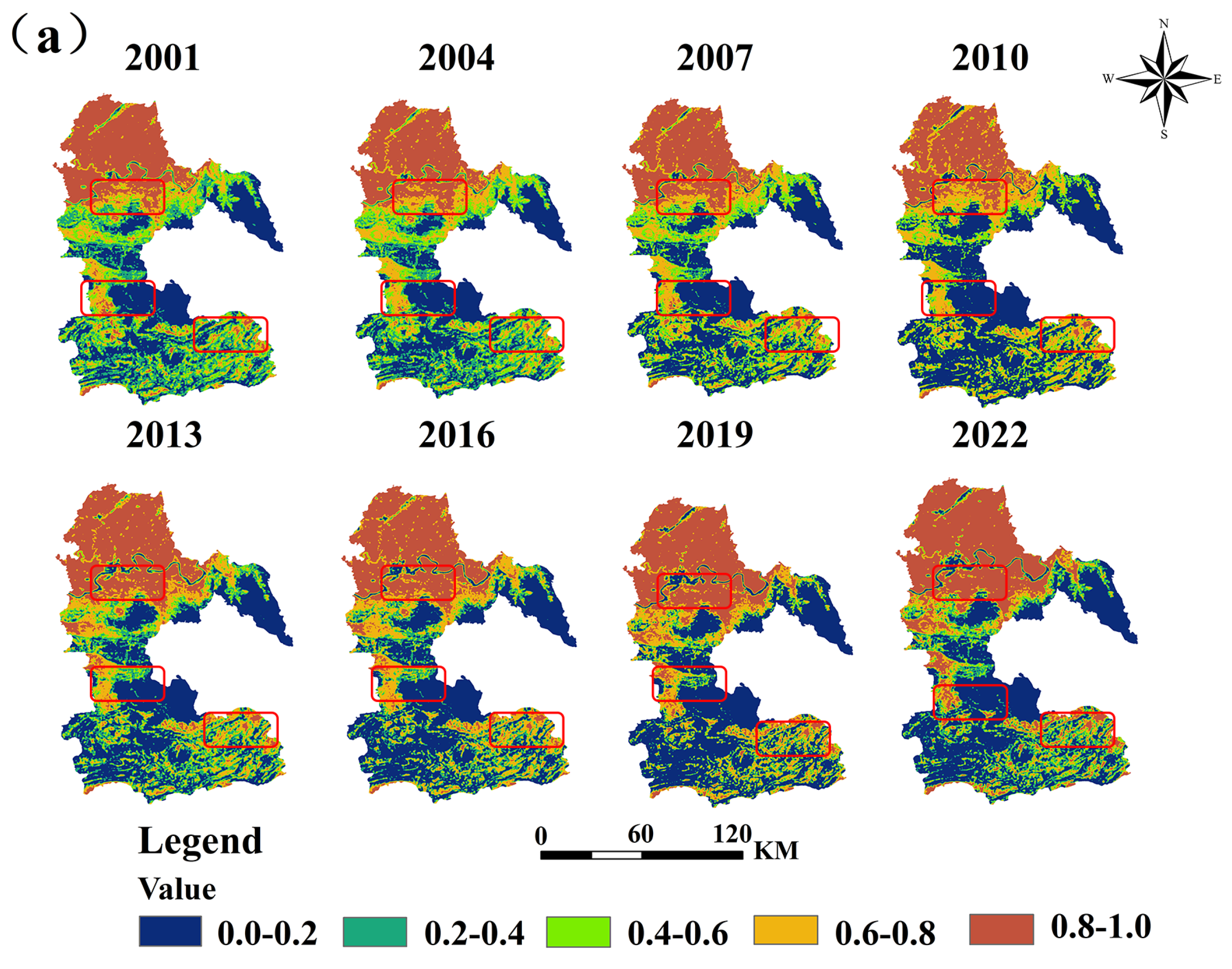
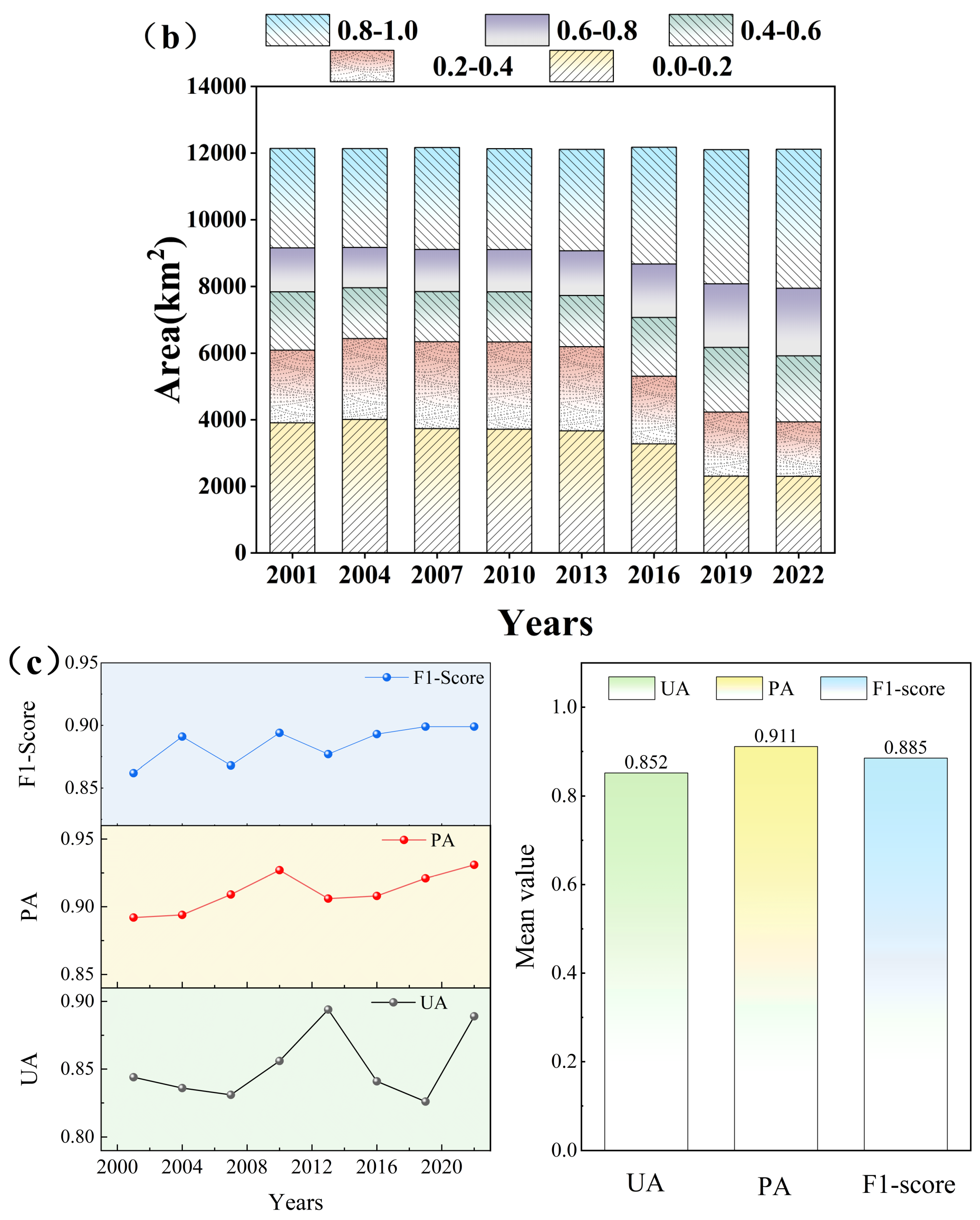
Using a random forest model and kernel density analysis with 23 feature variables, we generated annual arable land probability maps from 2000 to 2022 (Figure 5a) and produced a stacked area chart showing the probability distribution of different arable land grades over the same period (Figure 5b). We calculated User Accuracy (UA), Producer Accuracy (PA), and F1-scores [45], as shown in Figure 5c. The results show that the average UA, PA, and F1-score from 2001 to 2022 were 0.852, 0.911, and 0.885, respectively, meeting the accuracy requirements for this study. Spatially, high-probability arable land (≥0.8) was mainly concentrated in the northern part of the study area; relatively high-probability arable land (0.6–0.8) was predominantly distributed in the central and southern plains and the transitional zones between plains and low–mid mountains; and low-to-medium probability (<0.6) areas were mostly located in the south-central low–mid mountain region. Temporally, from 2000 to 2010, regions with medium-high to high probability (0.6–1.0) showed a slow contraction at an average annual rate of –0.69%, mainly in the boundary zone between plains and low–mid mountains. Medium-probability areas (0.4–0.6) exhibited a decreasing trend in 2004, with an average annual decrease of 1.87%, and experienced only minor fluctuations from 2004 to 2010. Low-probability areas (<0.4) displayed an increasing trend, with an average annual increase of 0.11%. During 2010–2013, changes were relatively small: areas with medium-high to high probability (0.6–1.0) increased slightly, while areas with medium or low probability (<0.6) decreased slightly. From 2013 to 2022, areas with medium-high to high probability (0.6–1.0) increased sharply, at an average annual rate of +4.65%, indicating intensified arable land use; medium-probability areas (0.4–0.6) grew slowly (+0.01% per year); and low-probability areas (<0.4) decreased dramatically, with an average annual decline of –3.10%. Overall, the spatial differentiation of arable land probability intensified: the stability of the core arable land area in the northern region increased, while uncertainty increased significantly in the marginal zones at the boundary between plains and low–mid mountains.

3.2. Spatiotemporal Dynamics of Cropland Abandonment

3.2.1. Extraction and Accuracy Validation of Abandoned Cropland

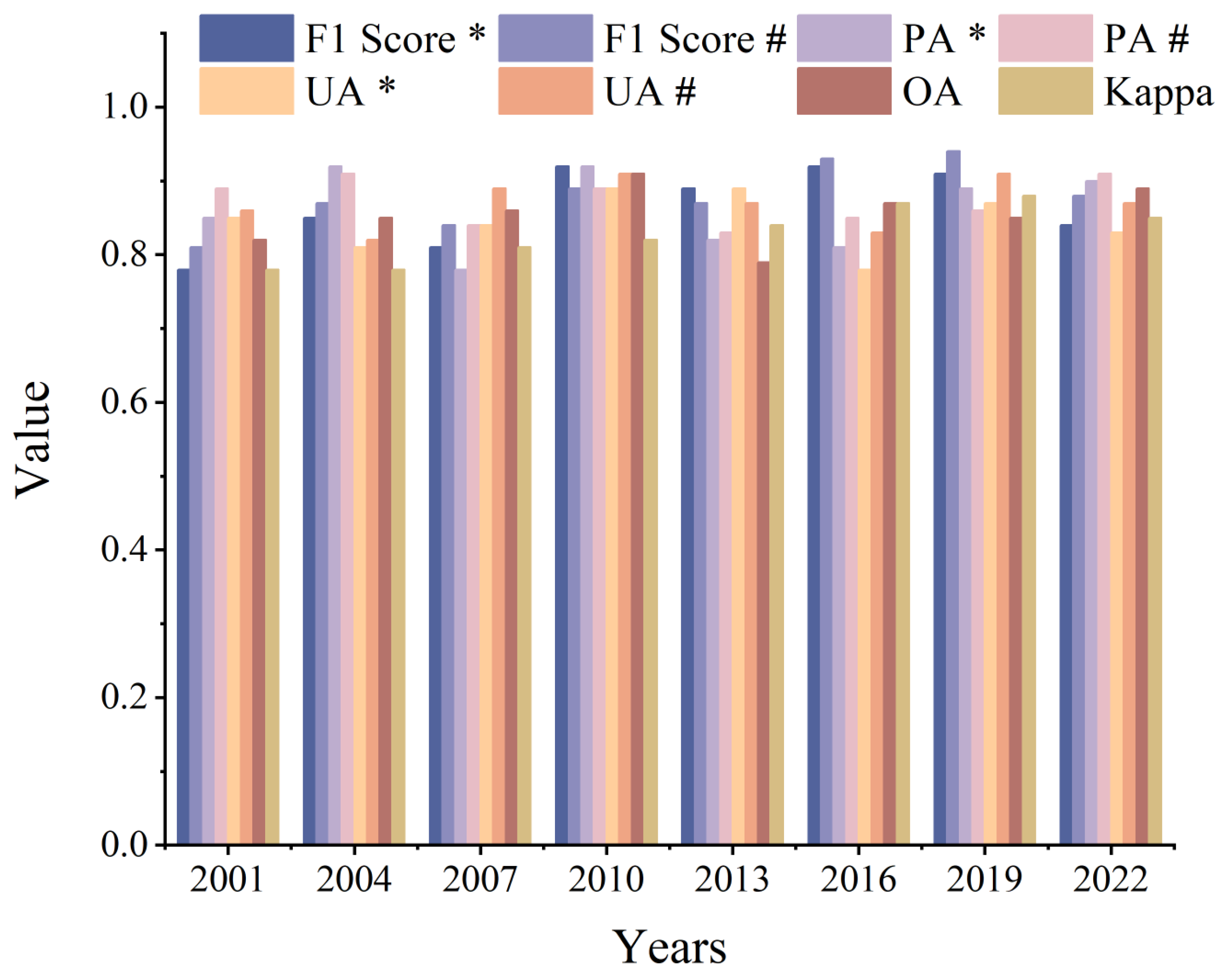
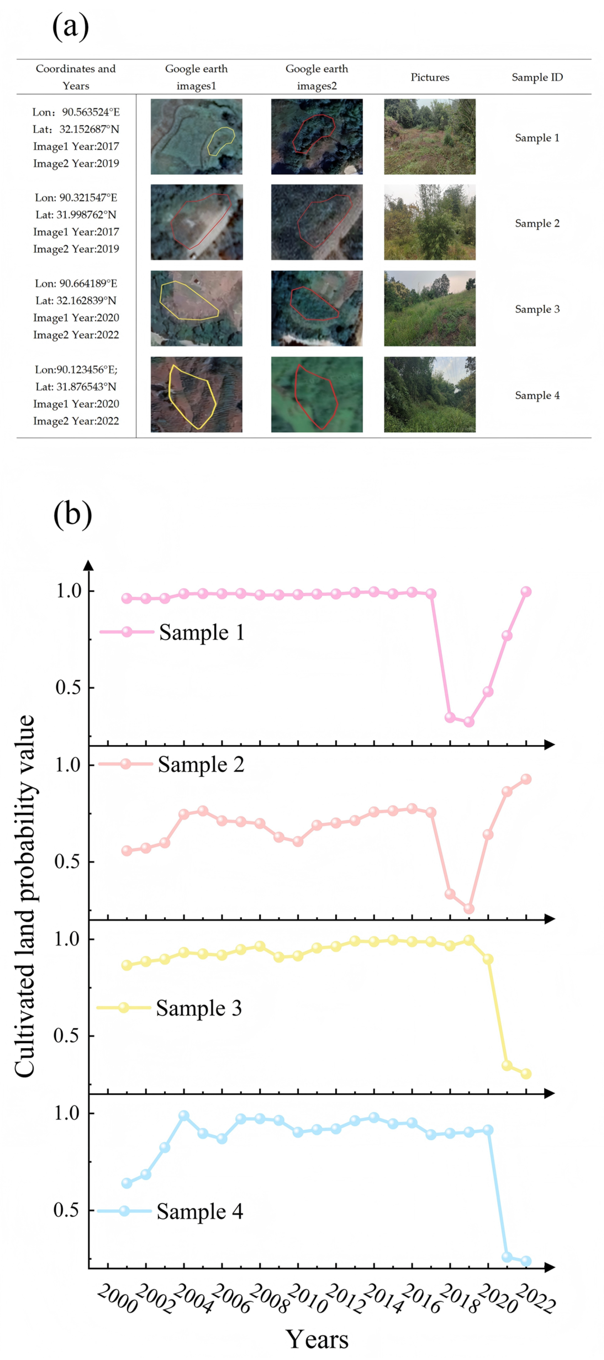
To assess accuracy, we performed annual confusion matrix analyses from 2000 to 2022. We calculated Overall Accuracy (OA), Kappa coefficients, F1-scores, Producer Accuracy (PA), and User Accuracy (UA). The mean OA was 0.855 (range: 0.798–0.910), and the mean Kappa was 0.828 (range: 0.780–0.886). The distribution map of mapping accuracy is shown in Figure 6. Among the accuracy metrics for abandoned cropland mapping, the F1-score presented the highest average value, while the mean UA was the lowest. Furthermore, all three accuracy indicators remained at a high level in 2004, 2010, 2016, and 2019. Furthermore, to validate the mapping results of abandoned cropland, we first compared them with cropland inflow and outflow data from the Provincial Department of Natural Resources, finding consistent trends in both area and spatial distributions. Second, we conducted field surveys across seven districts and counties of Luzhou City, using independent field samples for validation. Five typical abandoned cropland plots were selected for onsite verification in each district or county; partial field sample patch information is shown in Figure 7. The survey results showed strong agreement with the spatial identification results of this study, thereby confirming the reliability of the proposed method.

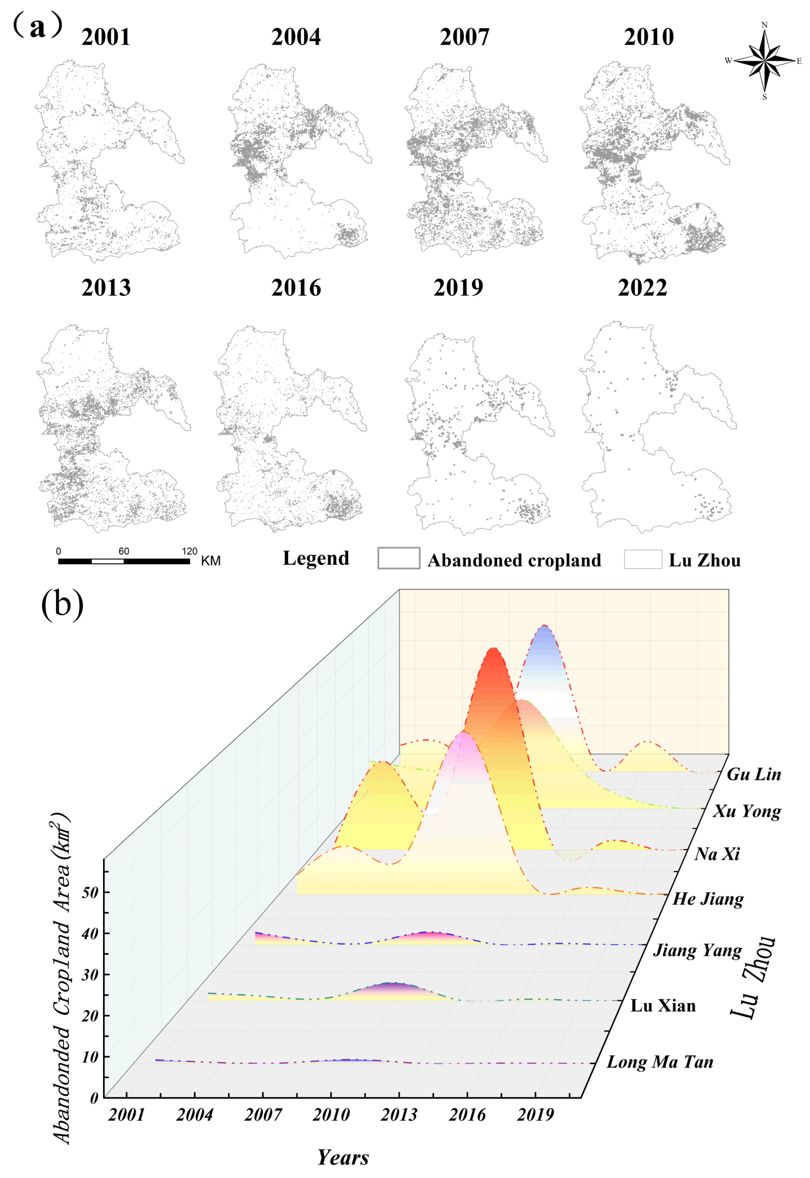
Figure 8 illustrates the distribution of abandoned cropland from 2000 to 2022. First, we applied LandTrendr to identify initial change patches. Second, patches that converted to built-up land were removed. Third, patches associated with short-term fallow or policy-driven retirement (e.g., the “Grain for Green” program) were excluded. The remaining patches represent spontaneously abandoned cropland. Spatially, abandoned cropland was mainly concentrated in the low-to-medium mountain areas of the southern study region [46]. Specifically, the abandoned areas in Gulin County, Xuyong County, Naxi District, and Hejiang County were substantially larger than those in the northern districts (Longmatan District, Lu County, and Jiangyang District). Taking the peak year of 2010 as an example, Naxi District had the largest abandoned area (63.22 km²), followed by Gulin County (50.32 km²), Hejiang County (48.45 km²), and Xuyong County (35.85 km²). In contrast, the abandoned areas in the northern districts were all below 5 km² (Longmatan: 0.98 km², Lu County: 4.79 km², and Jiangyang: 3.61 km²). Temporarily, the total abandoned area showed a pattern of initial increase followed by a decrease. From 2001 to 2010, it increased from 38.89 km² to 207.24 km², with an average annual increase of 18.71 km² and an average annual growth rate of 20.4%. Between 2010 and 2013, the area dropped sharply to 35.25 km², representing an average annual decrease of 57.33 km² and an average annual decline rate of 44.6%. From 2013 to 2021, the area decreased to 0.47 km², with an average annual decrease of 4.35 km² and an average annual decline rate of 24.7%, indicating that cropland abandonment had been effectively and consistently curbed after 2013. Overall, the risk of cropland abandonment was much higher in the southern mountainous areas than in the northern plains. However, after peaking in 2010, the total abandoned area across the city exhibited a rapid and sustained decreasing trend.

3.2.2. Spatiotemporal Clustering and Trends

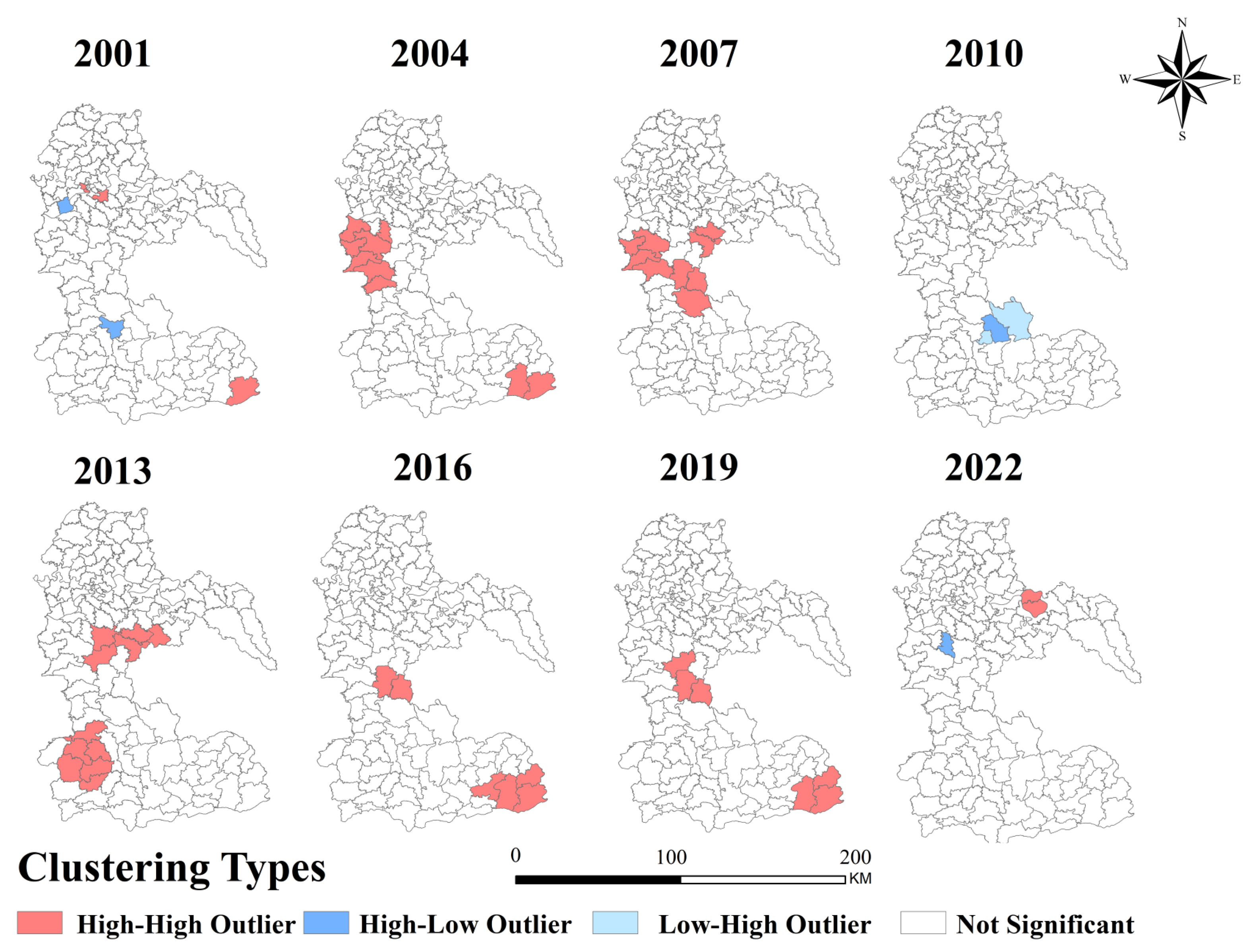
The spatial clustering of abandoned cropland in Luzhou was further examined using LISA (Local Indicators of Spatial Association) analysis at the township scale (Figure 9). The Global Moran’s I index remained consistently positive from 2000 to 2022, indicating statistically significant positive spatial autocorrelation. Over time, the distribution of significant clusters shifted markedly: from the central region in the early 2000s towards the central-southern region in later years. Specifically, High–High clusters (hotspots of abandonment) gradually expanded southward, while High–Low and Low–High outliers remained sporadic and locally constrained. Areas identified as “Not Significant” occupied most of the northern and western townships, suggesting that abandonment was less spatially structured in those areas.

3.3. Drivers of Cropland Abandonment

3.3.1. Analysis of Geodetector Results

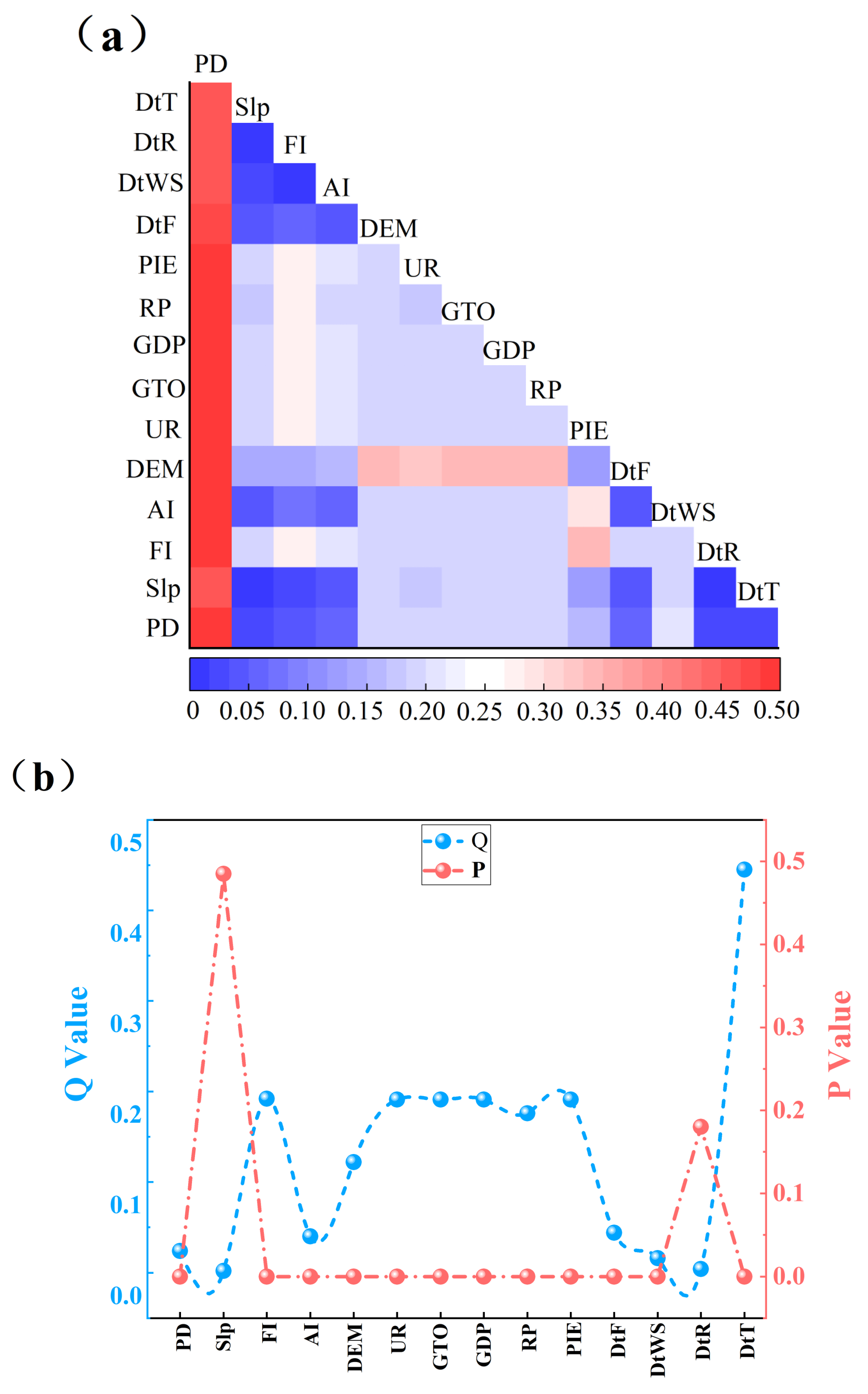
• Interaction Detector. This module assesses whether combining two factors improves their explanatory power. The results show that all two-factor interactions had higher q-values than single factors (Figure 10a). Most interactions showed nonlinear enhancement, and no antagonistic effects occurred. Distance to town (DtT) was the strongest interactive driver. It produced high q-values when paired with other factors. Specifically, the interactions of cropland fragmentation index (FI) with DtT and urbanization rate (UR) were the strongest. This indicates a strong synergistic effect among natural, socio-economic, and locational factors.
• Factor Detector. Figure 10b shows the explanatory power (q-value) of individual drivers. Distance to town (DtT) had the highest explanatory power. Other significant factors included cropland fragmentation index (FI), urbanization rate (UR), total grain output (GTO), GDP, rural population (RP), employment in the primary industry (PIE), and elevation (DEM). These variables are the key determinants of cropland abandonment in the study area.

3.3.2. Analysis of Drivers

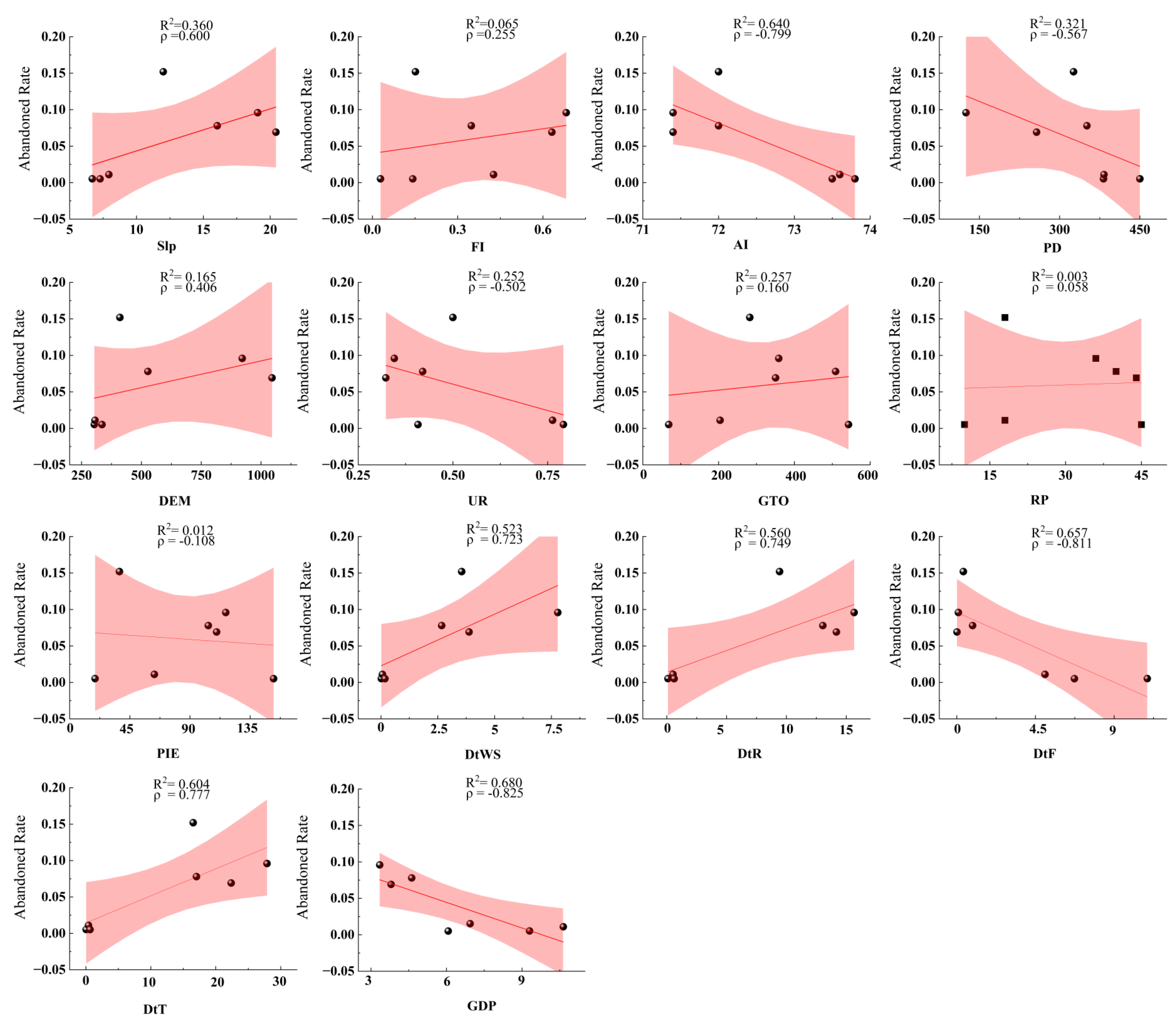
In this study, a linear regression model was used to quantify the association between cultivated land abandonment rate and 14 key drivers across districts and counties in the study area (Figure 11). Results showed significant heterogeneity in explanatory power (R²) and correlation ($\rho$) among factors. Distance to town centers (DtT) had the strongest positive correlation with abandonment rate, which is consistent with reduced cropland accessibility and lower agricultural input–output ratios. Distance to water sources (DtWS) was also positively correlated, highlighting the importance of irrigation for continuous land use. In contrast, GDP was negatively correlated with abandonment rate, indicating that higher economic development and more non-agricultural employment can suppress abandonment by improving agricultural efficiency and land transfer willingness. Distance to roads (DtR) was negatively correlated, confirming the role of transportation accessibility in reducing production costs and sustaining land use. Slope (Slp) and population density (PD) showed moderate correlations, while employment in the primary industry (PIE) had weak explanatory power. Overall, cropland abandonment in Luzhou is a complex process shaped by natural conditions, socio-economic factors, and location accessibility.

Furthermore, based on the comprehensive analysis of the geographical detector and linear regression, the main driving factors of abandoned cropland were found to be distance to town (DtT), total grain production (GTO), and GDP.

4. Discussion

4.1. Spatial Distribution of Abandoned Cropland

Dynamic monitoring of abandoned cropland in hilly and mountainous areas has long been challenging due to complex terrain and persistent cloud cover. Long-term studies spanning over two decades are further constrained by the availability and quality of suitable imagery. While Sentinel-1/2 satellites provide 10 m resolution data, their temporal coverage remains limited [27]. Landsat data offer a longer time span but require adapted extraction methods due to their coarser spatial resolution. The novel method developed in this study demonstrated its effectiveness for high-precision mapping in the hilly terrain of Luzhou City. Our results indicate that between 2000 and 2022, abandoned cropland in Luzhou was primarily concentrated in the central mountainous regions and the southern low-to-medium elevation hills. This finding differs from a previous study of cropland abandonment across Sichuan Province, which reported that abandoned cropland in Luzhou was mainly located in central mountainous and northern low-elevation areas [30]. To validate our results, we compared our findings with the Second and Third National Land Survey datasets and consulted the relevant literature [23,32]. The validation confirms that 72% of the uncultivated arable land is concentrated in the central and southern districts and counties (e.g., Hejiang, Xuyong, Gulin, and Naxi), which is consistent with our conclusions. Temporally, the abandoned cropland area in Luzhou showed a pattern of rapid initial increase followed by a fluctuating decline from 2000 to 2022. This trend aligns with the temporal dynamics observed in the neighboring city of Yibin, as reported in a study on cropland abandonment drivers in the Yangtze River Economic Belt [34,39]. Given the geographical proximity and similar topography, the comparable trends between the two cities further support our assessment. The abandonment area in Luzhou peaked around 2010, driven by rapid urbanization-induced rural population outflow and persistently low comparative benefits of agriculture. The sharp decline after 2013 coincided with the implementation of national cropland protection policies, including the cropland requisition–compensation balance system, high-standard cropland construction, comprehensive land consolidation, and the designation of permanent basic cropland. Since 2019, targeted measures have been further strengthened. Sichuan Province launched a special “dynamic clearance” campaign for abandoned cropland. By the end of 2022, Sichuan had restored approximately 2100 km² of cropland, of which Luzhou City accounted for about 220 km²—most of which came from the remediation of abandoned cropland.

4.2. Determinants of Cropland Abandonment

To identify the primary drivers of cropland abandonment and their influence, we integrated Geodetector and linear regression analyses. Both methods yielded consistent results. Based on these findings, we conclude that distance to towns (DtT), total grain output (GTO), and GDP are the decisive factors influencing abandonment. Integrating these results with local conditions in Luzhou explains the regional variations and underlying mechanisms. Spatially, high-quality cropland is concentrated along the Yangtze River and in the northern lowlands. In these regions, short distances to towns facilitate market access and service support; high grain output reflects productive agricultural systems; and higher GDP indicates strong local economies and abundant non-farm employment opportunities. These conditions create significant comparative advantages for agriculture, resulting in consistently high cultivation rates and minimal abandonment. In stark contrast, the southern region is characterized by long distances to towns, which severely limit accessibility to markets, inputs, and extension services; low total grain output reflects poor agricultural productivity; and low GDP indicates underdeveloped local economies and scarce non-farm job opportunities. The combination of these three factors drives labor migration to cities, reduces farmers’ motivation to cultivate, and leads to a very low input–output ratio. Consequently, the abandonment rate in the south is significantly higher than in the north. Therefore, the southern region represents a critical area for cropland protection and management. In addition, distance to forest was included as a locational factor because cropland parcels close to forest edges are more susceptible to wildlife disturbance, shading, and seed dispersal from woody vegetation, which collectively reduce cultivation viability and increase the likelihood of abandonment—particularly in fragmented hilly terrains.

It should be noted that the explanatory power of a given factor may differ substantially between univariate linear regression and Geodetector due to their different underlying assumptions. Univariate linear regression assumes a linear relationship between the independent variable and cropland abandonment, and thus captures only average monotonic trends. In contrast, Geodetector detects nonlinear stratified heterogeneity without a linearity assumption, making it sensitive to threshold effects and spatial clustering patterns that are not linear in nature. For example, primary-industry employment (PIE) and rural population (RP) exhibited very low R² values (0.013 and 0.003, respectively) in linear regression, indicating negligible linear associations. However, Geodetector yielded significant q-values of 0.22 and 0.21, respectively, suggesting that both factors have strong nonlinear or threshold-based impacts on the spatial pattern of abandonment. A plausible explanation is that abandonment increases sharply only when PIE falls below a certain critical level or when RP drops below a density threshold—a typical “nonlinear release effect” in mountainous labor-outflow regions. Linear regression fails to capture such thresholds, whereas Geodetector reveals them through stratified spatial analysis. Therefore, the two methods are complementary: regression quantifies linear trends, while Geodetector uncovers nonlinear spatial heterogeneity.

4.3. Policy Implications and Recommendations

Our study identified total grain output (GTO), distance to towns, and GDP as the main drivers of cropland abandonment. Based on these findings, we propose the following measures. First, improve farming conditions to boost yields. We should reduce fragmentation by merging plots, preferably near permanent basic cropland. Investments in soil quality, irrigation (e.g., canals), and field roads are essential to support mechanization. Land consolidation projects can also help restore abandoned land. Second, improve accessibility to address the issue of distance. Local governments should upgrade county and township roads. Increasing public transportation routes will also improve farmers’ access to markets. Third, increase economic returns. We suggest promoting large-scale farming through land leasing and cooperatives. Farmers should use e-commerce to boost sales. In mountainous areas, intercropping (e.g., fruit trees, tea) can diversify income without damaging topsoil. Rural tourism (e.g., farm stays) should also be encouraged to broaden market channels. Finally, strengthen enforcement and monitoring. We must publicize cropland protection policies and prohibit unauthorized land-use changes. Regular monitoring using personnel and drone patrols can enable early detection of abandonment.

4.4. Limitations and Future Perspectives

While our random forest model outperformed traditional extraction methods, several limitations remain regarding sample validation, spatial analysis units, and experimental validation. First, despite using high-resolution reference imagery, the difficulty of conducting extensive field surveys in Luzhou’s complex terrain means that some classification errors are unavoidable. Second, this study relied on pixel-based detection using the LandTrendr algorithm. Although we incorporated kernel density estimation to smooth the results and approximate parcel-level data, this is not as rigorous as object-oriented extraction. Third, a temporal mismatch exists in the driver analysis: road and river network data were derived from 2020, yet the study period spans 2000–2022. Major road and river networks in the study area have remained relatively stable over the past two decades (with no significant large-scale construction or rerouting), and thus, using the 2020 static dataset introduces only limited bias; we acknowledge that unrecorded local changes (e.g., new rural roads or small-scale river modifications) may cause certain underestimations or overestimations. This limitation has been discussed and should be addressed in future research. In future work, we aim to overcome the pixel-level limitation by developing a parcel-level analysis framework, which will further enhance the accuracy of cropland abandonment monitoring. More importantly, we recognize that the current study lacks systematic baseline comparisons and ablation experiments to validate the necessity of each component (e.g., combining random forest with kernel density estimation and LandTrendr). Therefore, we will prioritize these validations in our subsequent studies, including benchmarking against simpler methods (e.g., LandTrendr alone or RF alone) and performing component-wise ablation to quantify the performance gain of the proposed integrated framework. These steps are essential to rigorously demonstrate the added value of our methodology.

5. Conclusions

Monitoring abandoned cropland in hilly areas is vital for food security. We developed a new method to track these changes in Luzhou City from 2000 to 2022. We combined random forest, kernel density analysis, and the LandTrendr algorithm. Our results reveal a clear pattern: abandoned cropland exhibited an increasing trend from 2000 to 2010, with an average annual growth rate of 20.4%. From 2010 to 2013, the area of abandoned cropland declined rapidly, decreasing by 44.6%. Between 2013 and 2022, abandoned cropland decreased steadily, with an average annual reduction rate of 24.7%. Spatially, most abandoned cropland is located in the central and southern hilly mountainous areas. We further analyzed the driving factors and found that distance to towns (DtT), total grain output (GTO), and GDP are the decisive determinants of abandonment, with geographic location and economic conditions interacting to significantly influence cropland abandonment. These findings indicate that cropland abandonment strongly depends on transportation accessibility and economic development levels. Therefore, we recommend that future policies in the Yangtze River basin focus on improving road infrastructure and agricultural profitability in remote areas. Our framework provides a reliable tool for monitoring abandoned cropland in the hilly regions of southwestern China.

References

1. Jiang, G.; Wang, M.; Qu, Y.; Zhou, D.; Ma, W. Towards cultivated land multifunction assessment in China: Applying the “influencing factors-functions-products-demands” integrated framework. Land Use Policy 2020, 99, 104982. [Google Scholar] [CrossRef]
2. Yan, H.; Liu, F.; Qin, Y.; Niu, Z.; Doughty, R.; Xiao, X. Tracking the spatio-temporal change of cropping intensity in China during 2000–2015. Environ. Res. Lett. 2019, 14, 035008. [Google Scholar] [CrossRef]
3. Kong, X.; Chen, W.; Dang, Y. Current situation, challenges and transformation of cultivated land protection in China. J. Soc. Sci. Hunan Norm. Univ. 2023, 52, 31–41. [Google Scholar]
4. Khorchani, M.; Nadal-Romero, E.; Tague, C.; Lasanta, T.; Zabalza, J.; Lana-Renault, N.; Domínguez-Castro, F.; Choate, J. Effects of active and passive land use management after cropland abandonment on water and vegetation dynamics in the Central Spanish Pyrenees. Sci. Total Environ. 2020, 717, 137160. [Google Scholar] [CrossRef] [PubMed]
5. Alcantara, C.; Kuemmerle, T.; Baumann, M.; Bragina, E.V.; Griffiths, P.; Hostert, P.; Knorn, J.; Müller, D.; Prishchepov, A.V.; Schierhorn, F.; et al. Mapping the extent of abandoned farmland in Central and Eastern Europe using MODIS time series satellite data. Environ. Res. Lett. 2013, 8, 035035. [Google Scholar] [CrossRef]
6. Kurganova, I.; De Gerenyu, V.L.; Kuzyakov, Y. Large-scale carbon sequestration in post-agrogenic ecosystems in Russia and Kazakhstan. Catena 2015, 133, 461–466. [Google Scholar] [CrossRef]
7. Olsen, V.M.; Fensholt, R.; Olofsson, P.; Bonifacio, R.; Butsic, V.; Druce, D.; Ray, D.; Prishchepov, A. The impact of conflict-driven cropland abandonment on food insecurity in South Sudan revealed using satellite remote sensing. Nat. Food 2021, 2, 990–996. [Google Scholar] [CrossRef]
8. Alcantara, C.; Kuemmerle, T.; Prishchepov, A.V.; Radeloff, V.C. Mapping abandoned agriculture with multi-temporal MODIS satellite data. Remote Sens. Environ. 2012, 124, 334–347. [Google Scholar] [CrossRef]
9. Wang, S.; Di Tommaso, S.; Deines, J.M.; Lobell, D.B. Mapping twenty years of corn and soybean across the US Midwest using the Landsat archive. Sci. Data 2020, 7, 307. [Google Scholar] [CrossRef]
10. Wu, J.; Jin, S.; Zhu, G.; Guo, J. Monitoring of cropland abandonment based on long time series remote sensing data: A case study of Fujian Province, China. Agronomy 2023, 13, 1585. [Google Scholar] [CrossRef]
11. Wang, L.; Li, Q.; Wang, Y.; Zeng, K.; Wang, H. An OVR-FWP-RF Machine Learning Algorithm for Identification of Abandoned Farmland in Hilly Areas Using Multispectral Remote Sensing Data. Sustainability 2024, 16, 6443. [Google Scholar] [CrossRef]
12. Dong, J.; Xiao, X.; Menarguez, M.A.; Zhang, G.; Qin, Y.; Thau, D.; Biradar, C.; Moore, B., III. Mapping paddy rice planting area in northeastern Asia with Landsat 8 images, phenology-based algorithm and Google Earth Engine. Remote Sens. Environ. 2016, 185, 142–154. [Google Scholar] [CrossRef]
13. Shelestov, A.; Lavreniuk, M.; Vasiliev, V.; Shumilo, L.; Kolotii, A.; Yailymov, B.; Kussul, N.; Yailymova, H. Cloud approach to automated crop classification using Sentinel-1 imagery. IEEE Trans. Big Data 2019, 6, 572–582. [Google Scholar] [CrossRef]
14. Markert, K.N.; Markert, A.M.; Mayer, T.; Nauman, C.; Haag, A.; Poortinga, A.; Bhandari, B.; Thwal, N.S.; Kunlamai, T.; Chishtie, F.; et al. Comparing sentinel-1 surface water mapping algorithms and radiometric terrain correction processing in southeast asia utilizing google earth engine. Remote Sens. 2020, 12, 2469. [Google Scholar] [CrossRef]
15. Gorelick, N.; Hancher, M.; Dixon, M.; Ilyushchenko, S.; Thau, D.; Moore, R. Google Earth Engine: Planetary-scale geospatial analysis for everyone. Remote Sens. Environ. 2017, 202, 18–27. [Google Scholar] [CrossRef]
16. Xu, L.; Zhang, H.; Wang, C.; Zhang, B.; Liu, M. Crop classification based on temporal information using sentinel-1 SAR time-series data. Remote Sens. 2018, 11, 53. [Google Scholar] [CrossRef]
17. Moola, W.S.; Bijker, W.; Belgiu, M.; Li, M. Vegetable mapping using fuzzy classification of Dynamic Time Warping distances from time series of Sentinel-1A images. Int. J. Appl. Earth Obs. Geoinf. 2021, 102, 102405. [Google Scholar] [CrossRef]
18. Kennedy, R.E.; Yang, Z.; Cohen, W.B. Detecting trends in forest disturbance and recovery using yearly Landsat time series: 1. LandTrendr-Temporal segmentation algorithms. Remote Sens. Environ. 2010, 114, 2897–2910. [Google Scholar] [CrossRef]
19. Yimeng, G.; Shan, H.; Huaiyong, S. Extraction and spatiotemporal analysis of abandoned cultivated land in the Lower Reaches of Yellow River Basin using RF and LandTrendr algorithms. Trans. Chin. Soc. Agric. Eng. 2025, 41, 271–280. [Google Scholar] [CrossRef]
20. Chen, H.; Tan, Y.; Xiao, W.; Xu, S.; Xia, H.; Ding, G.; Xia, H.; Prishchepov, A.V. Spatiotemporal variation in determinants of cropland abandonment across Yangtze River Economic Belt, China. Catena 2024, 245, 108326. [Google Scholar] [CrossRef]
21. Zhou, H.; Wang, J.; Sun, M.; Wang, J.; Yang, K. Evolution of farmland abandonment research from 1993 to 2023 using CiteSpace-based scientometric analysis. J. Geovis. Spat. Anal. 2024, 8, 20. [Google Scholar] [CrossRef]
22. Qiu, B.; Yang, X.; Tang, Z.; Chen, C.; Li, H.; Berry, J. Urban expansion or poor productivity: Explaining regional differences in cropland abandonment in China during the early 21st century. Land Degrad. Dev. 2020, 31, 2540–2551. [Google Scholar] [CrossRef]
23. Zhang, Y.; Li, X.; Song, W. Determinants of cropland abandonment at the parcel, household and village levels in mountain areas of China: A multi-level analysis. Land Use Policy 2014, 41, 186–192. [Google Scholar] [CrossRef]
24. Zhang, T.; Yang, J.; Zhou, H.; Dai, A.; Gao, B.; Tang, K.; Tan, D. Abandoned Cropland Mapping with Phenology-Enhanced Change Vector Analysis and Semi-Supervised Learning in Different Cropping Intensity Areas. IEEE Trans. Geosci. Remote Sens. 2024, 62, 4404515. [Google Scholar] [CrossRef]
25. Liu, B.; Song, W. Mapping abandoned cropland using Within-Year Sentinel-2 time series. Catena 2023, 223, 106924. [Google Scholar] [CrossRef] [PubMed]
26. Hou, D.; Meng, F.; Prishchepov, A.V. How is urbanization shaping agricultural land-use? Unraveling the nexus between farmland abandonment and urbanization in China. Landsc. Urban. Plan. 2021, 214, 104170. [Google Scholar] [CrossRef]
27. Li, S.; Xiao, J.; Lei, X.; Wang, Y. Farmland abandonment in the mountainous areas from an ecological restoration perspective: A case study of Chongqing, China. Ecol. Indic. 2023, 153, 110412. [Google Scholar] [CrossRef]
28. Hong, C.; Prishchepov, A.V.; Bavorova, M. Cropland abandonment in mountainous China: Patterns and determinants at multiple scales and policy implications. Land Use Policy 2024, 145, 107292. [Google Scholar] [CrossRef]
29. He, S.; Shao, H.; Xian, W.; Yin, Z.; You, M.; Zhong, J.; Qi, J. Monitoring cropland abandonment in hilly areas with sentinel-1 and sentinel-2 timeseries. Remote Sens. 2022, 14, 3806. [Google Scholar] [CrossRef]
30. He, S.; Shao, H.; Xian, W.; Zhang, S.; Zhong, J.; Qi, J. Extraction of abandoned land in hilly areas based on the spatio-temporal fusion of multi-source remote sensing images. Remote Sens. 2021, 13, 3956. [Google Scholar] [CrossRef]
31. Yin, H.; Brandão, A., Jr.; Buchner, J.; Helmers, D.; Iuliano, B.G.; Kimambo, N.E.; Lewińska, K.E.; Razenkova, E.; Rizayeva, A.; Rogova, N.; et al. Monitoring cropland abandonment with Landsat time series. Remote Sens. Environ. 2020, 246, 111873. [Google Scholar] [CrossRef]
32. Hong, B.; Wang, J.; Xiao, J.; Yuan, Q.; Ren, P. Spatiotemporal Patterns and Determinants of Cropland Abandonment in Mountainous Regions of China: A Case Study of Sichuan Province. Land 2025, 14, 647. [Google Scholar] [CrossRef]
33. Jiang, L.; Wu, S.; Liu, Y. Change analysis on the spatio-temporal patterns of main crop planting in the middle yangtze plain. Remote Sens. 2022, 14, 1141. [Google Scholar] [CrossRef]
34. Kauth, R.J.; Thomas, G.S. The Tasselled Cap—A Graphic Description of the Spectral-Temporal Development of Agricultural Crops as Seen by LANDSAT. In Symposium on Machine Processing of Remotely Sensed Data; Purdue University: West Lafayette, IN, USA, 1976; pp. 159–167. [Google Scholar]
35. Li, Z.J.; Chen, G.F.; Zhi, J.W.; Xiang, Y.Z.; Li, D.M.; Zhang, F.C.; Chen, J.Y. Estimation model of soybean soil moisture content based on UAV spectral information and texture features. Nongye Jixie Xuebao 2024, 55, 347–357. [Google Scholar]
36. Hong, C.; Prishchepov, A.V.; Jin, X.; Zhou, Y. Mapping cropland abandonment and distinguishing from intentional afforestation with Landsat time series. Int. J. Appl. Earth Obs. Geoinf. 2024, 127, 103693. [Google Scholar] [CrossRef]
37. Rivai, F.A.; Tjahjono, B.; Munibah, K.; Nofrizal, A.Y. Majority filter for enhancing pixel-based random forest land cover classification in Sukajaya District, Bogor Regency. Geogr. Environ. Sustain. 2025, 18, 171–182. [Google Scholar] [CrossRef]
38. Liu, Y.; Chen, Y.; Wu, Z.; Wang, B.; Wang, S. Geographical detector-based stratified regression kriging strategy for mapping soil organic carbon with high spatial heterogeneity. Catena 2021, 196, 104953. [Google Scholar] [CrossRef]
39. Liu, D.; Chen, N.; Zhang, X.; Wang, C.; Du, W. Annual large-scale urban land mapping based on Landsat time series in Google Earth Engine and OpenStreetMap data: A case study in the middle Yangtze River basin. ISPRS J. Photogramm. Remote Sens. 2020, 159, 337–351. [Google Scholar] [CrossRef]
40. Breiman, L. Random forests. Mach. Learn. 2001, 45, 5–32. [Google Scholar] [CrossRef]
41. Crawford, C.; Yin, H.; Radeloff, V.; Wilcove, D. Rural land abandonment is too ephemeral to provide major benefits for biodiversity and climate. Sci. Adv. 2022, 8, eabm8999. [Google Scholar] [CrossRef] [PubMed]
42. Guo, A.; Yue, W.; Yang, J.; Xue, B.; Xiao, W.; Li, M.; He, T.; Zhang, M.; Jin, X.; Zhou, Q. Cropland abandonment in China: Patterns, drivers, and implications for food security. J. Clean. Prod. 2023, 418, 138154. [Google Scholar] [CrossRef]
43. Stolzenberg, R.M. Multiple regression analysis. In Handbook of Data Analysis; Handbook of Data Analysis; SAGE Publications, Ltd.: London, UK, 2004; pp. 165–208. [Google Scholar] [CrossRef]
44. Powers, D.M. Evaluation: From precision, recall and F-measure to ROC, informedness, markedness and correlation. arXiv 2020, arXiv:2010.16061. [Google Scholar] [CrossRef]
45. Chen, H.; Tan, Y.; Xiao, W.; He, T.; Xu, S.; Meng, F.; Li, X.; Xiong, W. Assessment of continuity and efficiency of complemented cropland use in China for the past 20 years: A perspective of cropland abandonment. J. Clean. Prod. 2023, 388, 135987. [Google Scholar] [CrossRef]
46. Xu, X.L. China Multi-Year Provincial Administrative Division Boundary Dataset. Resource and Environment Science Data Registration and Publication System. 2023. Available online: https://www.resdc.cn/DOI/doi.aspx?DOIid=122 (accessed on 2 January 2025).
Figure 1. Geographic location and topography of the study area.
Remotesensing 18 01562 g001
Figure 2. The spatial distribution of the number of available images.
Remotesensing 18 01562 g002
Figure 3. Technical framework for monitoring and attribution analysis of cropland abandonment.
Remotesensing 18 01562 g003
Figure 4. Sample point distribution map (In the Figure, the square-style legend represents inter-annual cropland samples, and the circular-style legend represents inter-annual other samples.).
Remotesensing 18 01562 g004
Figure 5. Spatial–temporal patterns and mapping accuracy of cropland probability in Luzhou City from 2000 to 2022. (a) Evolution of cropland probability spatial distribution (the red-circled region in the Figure indicates significant change); (b) area distribution map of probability values for different grades of cropland from 2000 to 2022; and (c) cropland probability mapping accuracy.
Remotesensing 18 01562 g005aRemotesensing 18 01562 g005b
Figure 6. Mapped accuracy of abandoned cropland. * is the abandoned cropland, and # is the other land category.
Remotesensing 18 01562 g006
Figure 7. Comparison among random field samples. (a) Google Earth images, and extracted abandonment samples; (b) random field samples’ inter-annual curve of cropland probability.
Remotesensing 18 01562 g007
Figure 8. (a) Distribution map of abandoned cropland, 2000–2022; (b) inter-annual variation in abandoned cropland area by district/county.
Remotesensing 18 01562 g008
Figure 9. Local Indicators of Spatial Association (LISA) cluster distribution at the township scale.
Remotesensing 18 01562 g009
Figure 10. Detection results of drivers’ explanatory power. (a) Interaction between driving factors; (b) individual factors on cropland abandonment rate.
Remotesensing 18 01562 g010
Figure 11. Linear regression relationships between the cultivated land abandonment rate and 14 key driving factors across districts and counties in Luzhou. Each subplot shows the association between the abandonment rate and a specific factor, with the coefficient of determination ( R 2 ) and the Pearson correlation coefficient ( ρ ) provided. The red line represents the linear regression fit, and the shaded area indicates the 95% confidence interval.
Remotesensing 18 01562 g011