Article

Pre-Launch Calibration and Performance Evaluation of OMS-N Onboard the FY-3F Satellite

1
National Space Science Center, Chinese Academy of Sciences, Beijing 100190, China
2
Beijing Key Laboratory of Space Environment Exploration, Beijing 100190, China
3
School of Astronomy and Space Science, University of Chinese Academy of Sciences, Beijing 100049, China
4
Shanghai Institute of Satellite Engineering, Shanghai 201109, China
5
National Key Laboratory of Scattering and Radiation, Beijing 100854, China
6
Beijing Institute of Space Mechanics & Electricity, Beijing 100194, China
7
National Satellite Meteorological Centre, Beijing 100081, China
*
Author to whom correspondence should be addressed.
Remote Sens. 2026, 18(10), 1456; https://doi.org/10.3390/rs18101456
Submission received: 27 February 2026 / Revised: 29 April 2026 / Accepted: 29 April 2026 / Published: 7 May 2026
(This article belongs to the Section Satellite Missions for Earth and Planetary Exploration)

Highlights

What are the main findings?
  • A full-dimensional ground calibration covering radiometric, spectral, and geometric aspects was completed for the OMS-N payload onboard the FY-3F satellite. The absolute radiometric calibration uncertainty was better than 2.33% for the UV channels and better than 1.69% for the VIS channel. The spectral wavelength error was ≤0.01 nm for the VIS channel. All performance indicators met or exceeded the design requirements.
  • Pixel-level parametric models were established for the spectral, spatial, and radiometric response distributions of OMS-N. The detector nonlinearity, dynamic range, and calibration uncertainty were systematically evaluated. The major sources of calibration errors for each channel were identified and quantified.
What are the implications of the main findings?
  • The results provide a technical foundation for OMS-N to conduct on-orbit quantitative remote sensing observations of global atmospheric ozone, trace gases, and other atmospheric constituents, supporting the stable generation of high-quality operational on-orbit data.
  • The established calibration methods and technical framework provide a standardized reference for the ground calibration of similar ultraviolet hyperspectral remote sensing instruments. They also contribute to improving the technical capabilities and data quality of atmospheric remote sensing monitoring in China.

Abstract

The Ozone Monitor Suite-Nadir (OMS-N) onboard the FY-3F satellite is a key payload for global atmospheric ozone and trace gas detection. The data quality depends on the accuracy of ground calibration. This study presents a systematic ground calibration of OMS-N. The instrument operates over 250–500 nm, with a spatial resolution of 7 × 7 km2 and a spectral resolution of 0.5–1 nm. Radiometric calibration was performed using an integrating sphere, spectral calibration using a tunable laser, and geometric calibration using a precision turntable. All tests were conducted under controlled environmental conditions (20 ± 3 °C and 50% ± 10% humidity). The absolute radiometric calibration uncertainty was below 2.33% for UV1/UV2 and 1.69% for VIS, with relative uncertainties ≤1.84%. The spectral wavelength error was ≤0.01 nm for the VIS channel and ≤0.03 nm for the UV1/UV2 channels, and the geometric positioning uncertainty was better than 0.1 pixels. All performance indicators met or exceeded the design requirements. These results provide technical support for the quantitative application of OMS-N data in atmospheric monitoring and establish a reference framework for the ground calibration of similar ultraviolet hyperspectral instruments.

1. Introduction

Environmental issues, such as atmospheric ozone depletion, global warming, and acid rain, represent some of the most critical challenges facing humanity in the 21st century [1,2]. Despite its relatively low atmospheric concentration, the ozone layer provides a natural shield for humans and other organisms. Anthropogenic depletion of the ozone layer has raised serious global concerns in recent decades, mainly due to industrial activities at higher altitudes. The discovery of the Antarctic ozone hole [3] served as a wake-up call. As ozone is a key greenhouse gas, monitoring its spatiotemporal variability has become a major focus of environmental remote sensing. Satellite-based ozone detection has been widely adopted because it enables global coverage in all weather conditions.
Among the most advanced low-orbit meteorological satellites, China’s FY-3 series [4,5,6,7,8] provides multispectral, global, all-weather, three-dimensional, and quantitative observations of surface, atmospheric, and oceanic parameters. The FY-3F satellite employs state-of-the-art quantitative remote sensing technology and carries onboard sensors, significantly enhancing detection accuracy. In addition to supporting emergency response and disaster mitigation, FY-3F, in conjunction with other FY-3 satellites, enables continuous global weather monitoring, thereby improving forecast precision and timeliness.
Launched on 3 June 2008, the Total Ozone Unit (TOU) aboard FY-3A [9,10,11] marked China’s first mission for quantitative global ozone detection, with retrieved ozone products achieving accuracy comparable to leading international payloads. Building on the success of the UV ozone sounders onboard FY-3A, FY-3B, and FY-3C, the Ozone Monitor Suite–Nadir (OMS-N) was developed. This instrument measures nadir ozone, aerosol optical thickness, cloud-top properties, air pressure, trace gases related to ozone and atmospheric composition (such as SO2, NO2, BrO, HCHO, and OClO), and total ozone. The inclusion of nadir pressure and ozone measurements has strengthened China’s capability for environmental monitoring, improved weather forecasting, and supported global climate research. This paper is organized as follows. Section 1 provides an introduction. Section 2 describes the instrument, and Section 3 introduces the calibration facilities and their characteristics. Section 3 present the OMS-N ground calibration results. Section 5 summarizes the study and outlines future perspectives.

2. Methods

2.1. Instrument Description

OMS-N is a spaceborne nadir-viewing push-broom imaging spectrograph equipped with two spectrometers covering both ultraviolet and visible bands. It measures backscattered radiation at the top of the atmosphere from the Earth’s surface and atmosphere using passive remote sensing. With a swath width of 112° and a polar orbit altitude of 836 km onboard FY-3F, OMS-N achieves a ground swath of approximately 2600 km and enables daily global coverage. The entire swath is imaged simultaneously onto two-dimensional (2D) detectors: one dimension records the cross-track spatial information, and the other captures the spectral data at each spatial location. The primary specifications of OMS-N are summarized in Table 1.
The OMS-N instrument employs a telescope to focus incident radiation from the target area onto a homogenizer slit, which serves as the entrance to the spectrometer. To achieve a larger entrance pupil for enhanced energy collection, the telescope adopts an image-side telecentric design and is equipped with two independent spectrometric channels. This configuration enables precise light collection and spectral analyses. With a field of view of 112°, the system incorporates three spectral channels: UV1 (250–300 nm), UV2 (300–320 nm), and VIS (310–495 nm). Two high-sensitivity CCD detectors were used to enhance the measurement accuracy and stability. UV1 and UV2 shared the same CCD detector, and binning was applied to UV1 to improve its signal-to-noise ratio (SNR).
On-orbit calibration is supported by a white light source (WLS) and two solar diffusers. By switching the calibration unit, the telescope optical path can be directed toward the Earth, the Sun, or other calibration sources. A schematic diagram of OMS-N is shown in Figure 1.
Figure 1 illustrates the working principle of OMS-N for on-orbit nadir and solar observations. The optical bench and detector module were passively cooled, with operating temperatures of 293.15 ± 2 K and −243 ± 0.1 K, respectively.

2.2. Calibration Approach

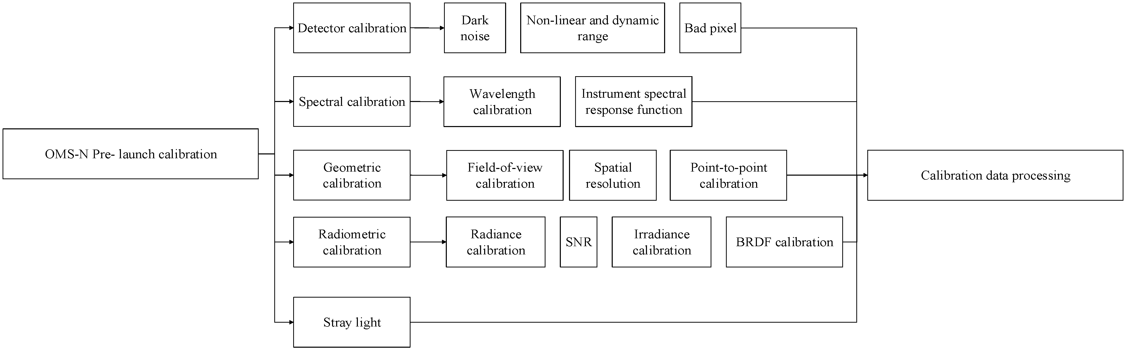
OMS-N requires pre-calibration against known radiometric sources to enable the retrieval of absolute atmospheric constituent densities. During on-orbit operations, relative calibration is conducted with respect to the Sun. The accuracy of OMS-N products depends on high-quality Level 1 (L1) data, which in turn relies on precise pre-launch ground calibration. Given the 2D CCD detector design, ground calibration should replicate on-orbit conditions and provide pixel-level calibration for radiometric, spectral, and geolocation parameters, making it a technically complex process. The OMS-N calibration workflow is shown in Figure 2.
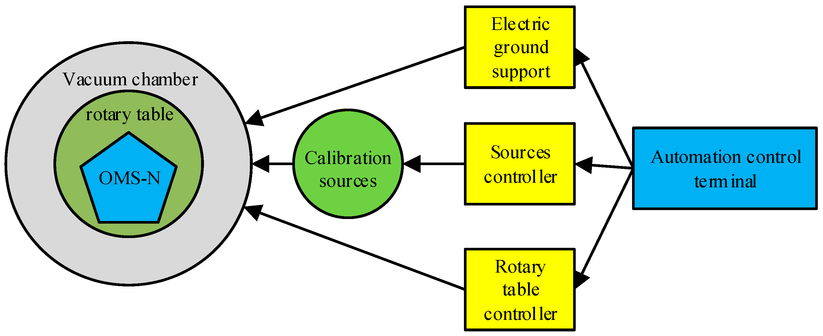
To better evaluate the on-orbit performance of OMS-N, all ground calibrations were conducted in a vacuum environment. Ground calibration was performed by the Beijing Institute of Space Mechanics and Electricity (BSME) in a 7.5 m thermal vacuum chamber located in a Class 10,000 clean room between October 2022 and January 2023. A liquid-nitrogen-cooled thermal shroud ensured a stable operating temperature. The instrument was mounted on a five-dimensional adjustment platform to allow full coverage of the field of view. The chamber was equipped with a 20 cm diameter UV-transmissive window, enabling sequential illumination across all swath angles by rotating the instrument. Calibration included both the Earth-port and Sun-port configurations, with the chamber maintained at Class 1000 cleanroom standards. An overview of the calibration setup is presented in Figure 3.

3. Results

3.1. Spectral Calibration

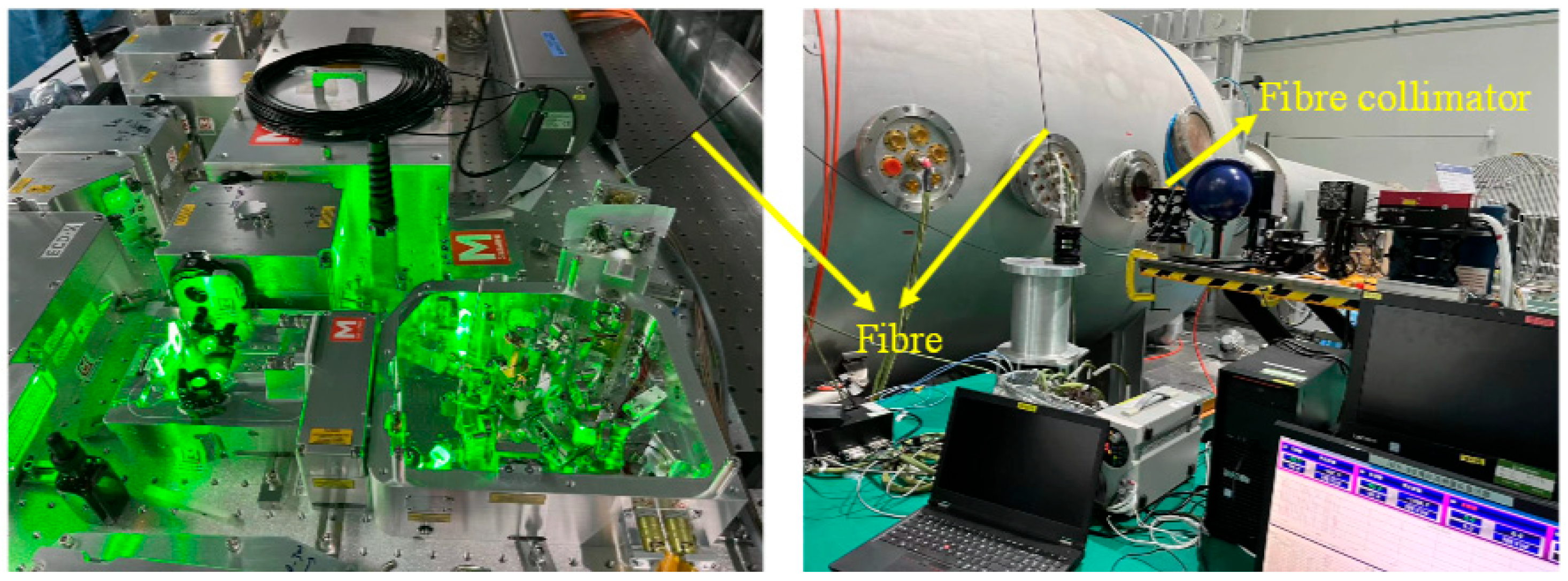
Spectral calibration consists of two components: wavelength calibration and measurement of the instrument spectral response function (ISRF). Wavelength calibration was performed to determine the spectral range and central wavelength of each detector element. For the OMS-N spectrometers, calibration was conducted using M-Squared tunable lasers (M Squared Lasers Ltd., Glasgow, UK) introduced into the instrument via fiber and collimator optics. The laser light was diffusely reflected within the OMS-N optical system, covering the full field of view and enabling pixel-level calibration by varying the laser wavelength. The experimental setup is illustrated in Figure 4.
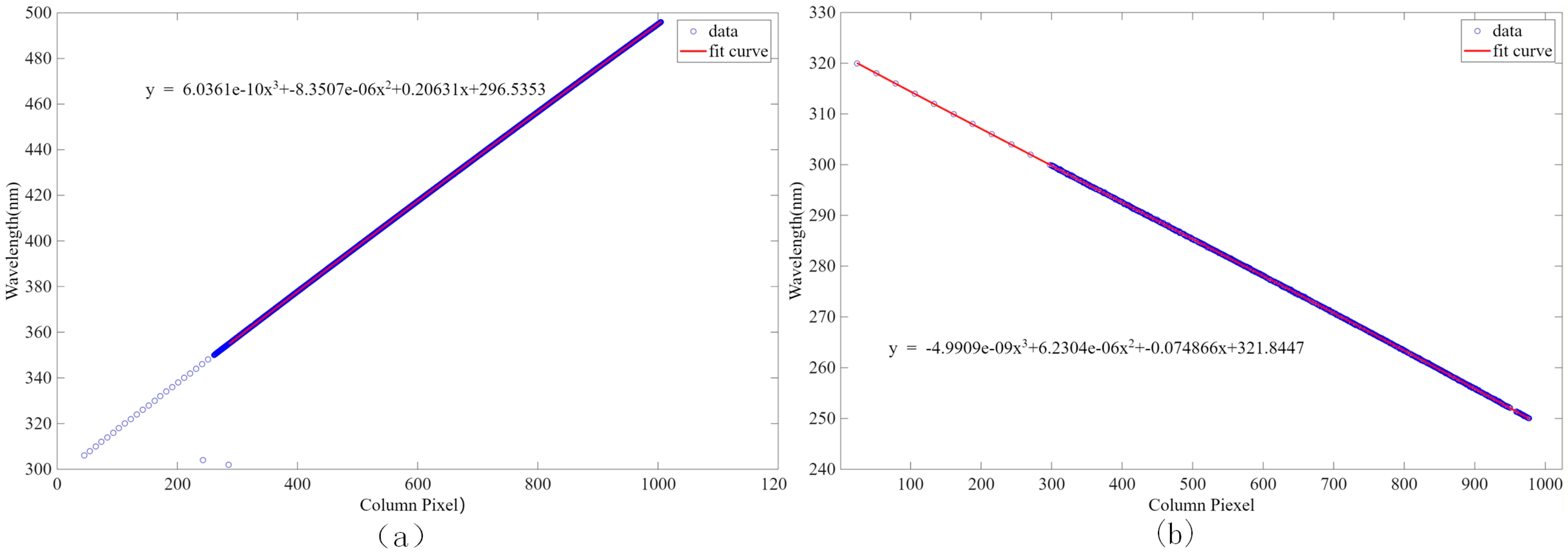
During spectral calibration, the M-Squared system supports only the spectral ranges of 250–300 nm and 350–500 nm and provides narrow linewidth and fine wavelength tuning. Therefore, for the 300–350 nm range spanning the UV2 and VIS channels, an optical parametric oscillator OPO laser (OPOTEKCarlsbad, CA, USA) with a tuning step of 2 nm was used, as shown in Figure 5. In the VIS channel, the laser wavelength was incremented in 0.02 nm steps, whereas the UV1 and UV2 channels were adjusted in 0.05 nm steps. Along one spatial dimension (rows), the spectra were fitted to determine the relationship between pixel serial number and central wavelength. Polynomial fitting was used to derive the calibration equations, and row-to-row variations resulted in distinct equations. The maximum root mean square error (RMSE) was 0.06 nm for the UV1 and UV2 channels and 0.03 nm for the VIS channel, and the correlation coefficients for all channels were greater than 0.99. The representative calibration equations for the UV and VIS channels are presented in Figure 5, and the wavelength distribution across the entire image plane was obtained by applying the calibration equation to each spatial row. The OPO laser exhibited instability at 302 and 304 nm during the tests, leading to a mismatch between the measured and nominal wavelengths. This resulted in two outliers near 300 nm, as shown in Figure 5a. Accordingly, polynomial fitting was performed starting from 306 nm to ensure the accuracy of the calibration model.
Calibration accuracy was verified using a mercury spectral lamp. Strong and isolated emission lines between 250 and 500 nm were selected for validation. The spectral response of the mercury lamp on the CCD detector was recorded, and the corresponding wavelengths were calculated using a calibration equation. Deviations were determined by comparing the calculated values with standard characteristic wavelengths. The wavelength calibration deviations are summarized in Table 2, showing a total deviation of less than 0.03 nm.
The instrument spectral response function (ISRF), also referred to as the slit function, characterizes the spectral response of each detector pixel at different wavelengths and can be expressed as R(xpixel, Δλ). Within this framework, the wavelength corresponding to a given pixel is defined as the response center. Each channel exhibits a distinct ISRF shape determined by its optical components, dispersive elements, and entrance slits. Because the spectrometer is equipped with a homogenizer slit, the ISRF is described by Equations (1) and (2). During the fitting process, multiple observations collected at the same wavelength were averaged and normalized. A pixel-specific ISRF model was established for each detector pixel for spectral calibration. The ISRF for the VIS channel is described by Equation (1).
y = n = 1 n = 8 a n e ( ( x b n ) c n ) 2
where a ( n ) represents the sub-function amplitude, b ( n ) represents the central peak of each subfunction, c ( n ) denotes the half-width correlation of subfunctions, x represents the pixel index, and y represents the wavelength.
Similarly, the ISRF for the UV channel is described by Equation (2):
y = a _ 1 + a _ 2 e ( c _ 1 ( x b ) ) 2 + ( c _ 2 ( x b ) ) 4 + ( c _ 3 ( x b ) ) 6 + ( c _ 4 ( x b ) ) 8
where a _ 1 represents the baseline of the function, a _ 2 represents the sub-function amplitude, b represents the central peak, c _ 1 c _ 4 represent the coefficients associated with the full width at half maximum (FWHM), x represents the pixel index, and y represents the wavelength.
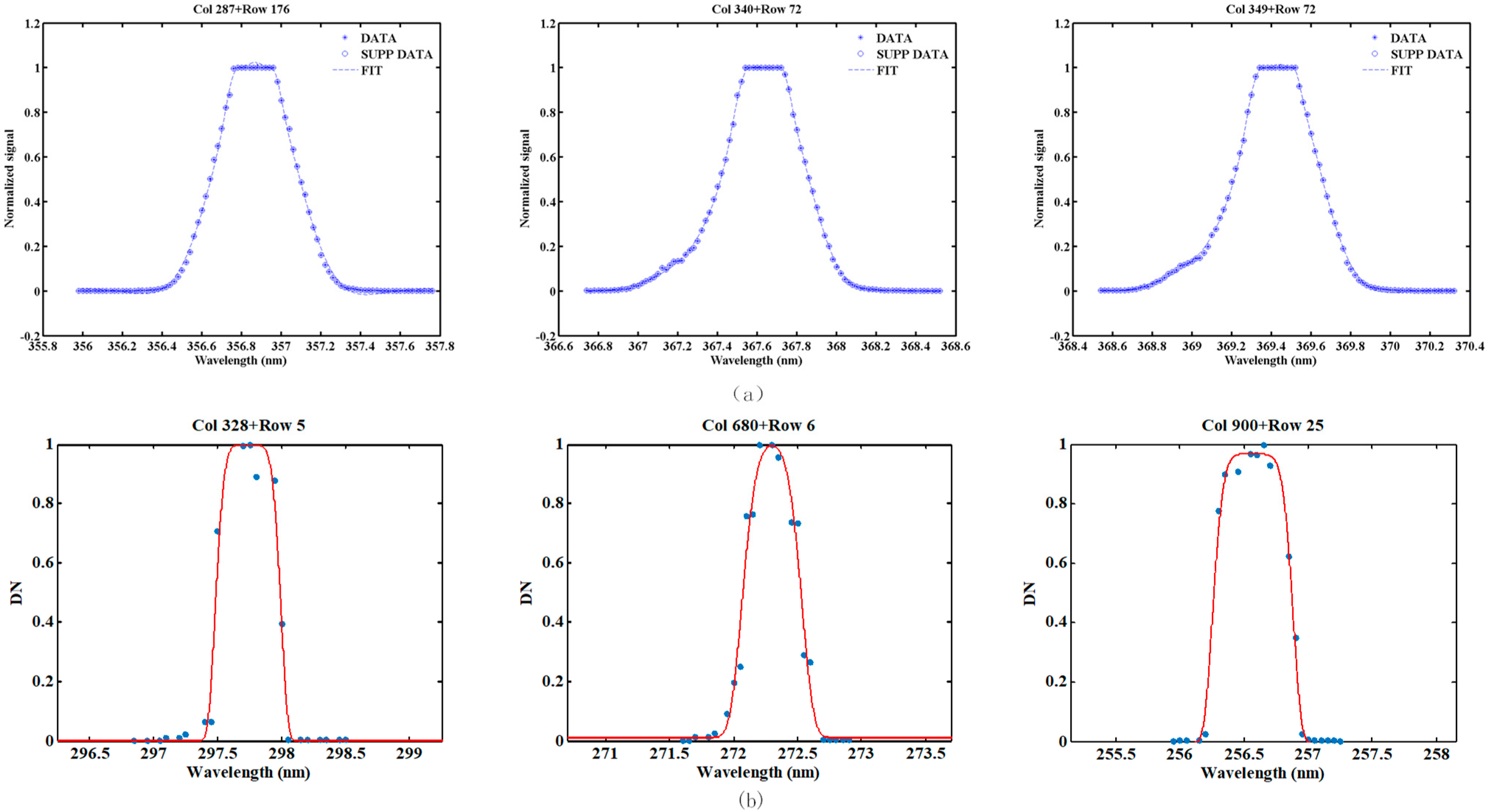
The ISRF was measured using an M-Squared tunable laser, following the wavelength step sizes specified in Section 4 (250–300 and 350–500 nm). The ISRF for each pixel was obtained after normalization. Representative ISRFs for the selected pixels from both channels are shown in Figure 6. The results indicate that, although minor variations exist across the field of view, the ISRFs for pixels within the same field are highly consistent. For the 300–350 nm range, extrapolated values were used to derive the ISRF.
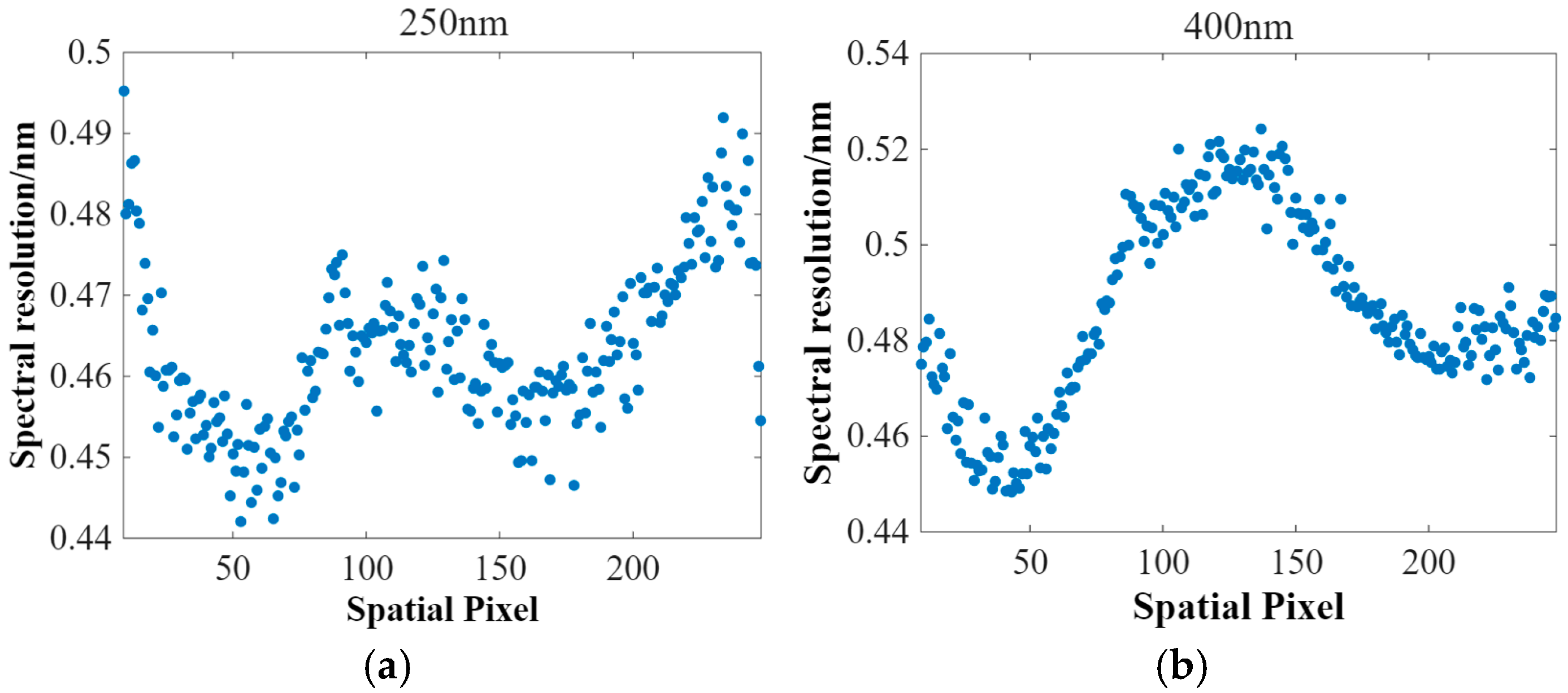
The ISRFs for OMS-N exhibited flat-topped shapes. The FWHM ranged from 0.45 to 0.50 nm for the UV1 and UV2 channels and from 0.50 to 0.60 nm for the VIS channel. Because UV1 and UV2 share a single CCD detector, the same binning factor was applied when calculating the spectral resolution. The spatial variation in spectral resolution was shown at 250 nm for the UV1 channel and at 400 nm for the VIS channel as shown in Figure 7. The results indicate that the spectral resolution at a given wavelength varies across the field of view. Therefore, a pixel-specific spectral response model was established to ensure accurate retrieval in subsequent applications.

3.2. Geometric Calibration

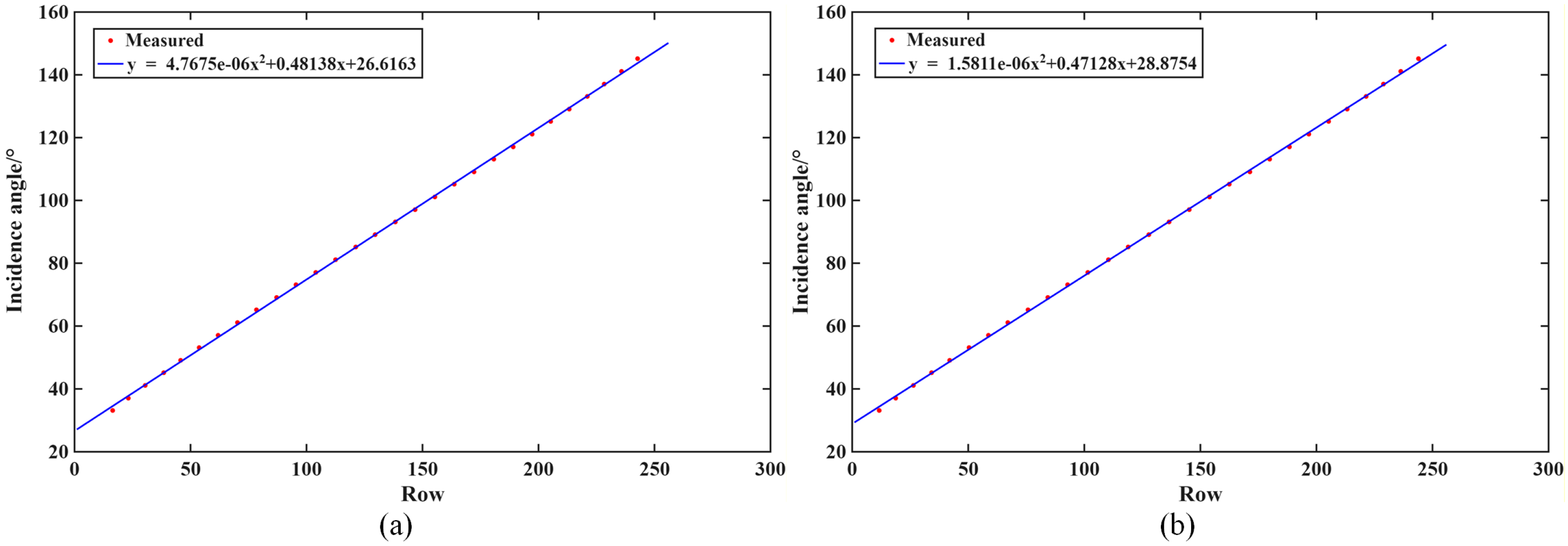
The total field of view (FOV) represents the maximum viewing angle of OMS-N in the orbital direction and was designed to be 112°. The FOV calibration method is analogous to spectral calibration. A large-diameter UV-collimated light source was used to illuminate the instrument at different incidence angles, and linear regression was applied to establish the relationship between the line pixel index and the corresponding incidence angle recorded by the CCD. The incidence angles of the first and last line pixels were defined as the boundaries of the instrument’s field of view, thereby completing calibration. For each spectral column, a polynomial fit was applied to relate the OMS-N incidence angle (An) to the spatial row, yielding FOV calibration equations (Figure 8). The fitting RMSEs were 0.10° for the UV1 and UV2 channels and 0.07° for the VIS channel, with correlation coefficients R greater than 0.99 for all channels.
y = 4.5755x2 − 0.18318x + 26.6163
y = 1.5811x2 + 66.47128x + 28.8754
where x represents the pixel index, and y represents the incident angle.
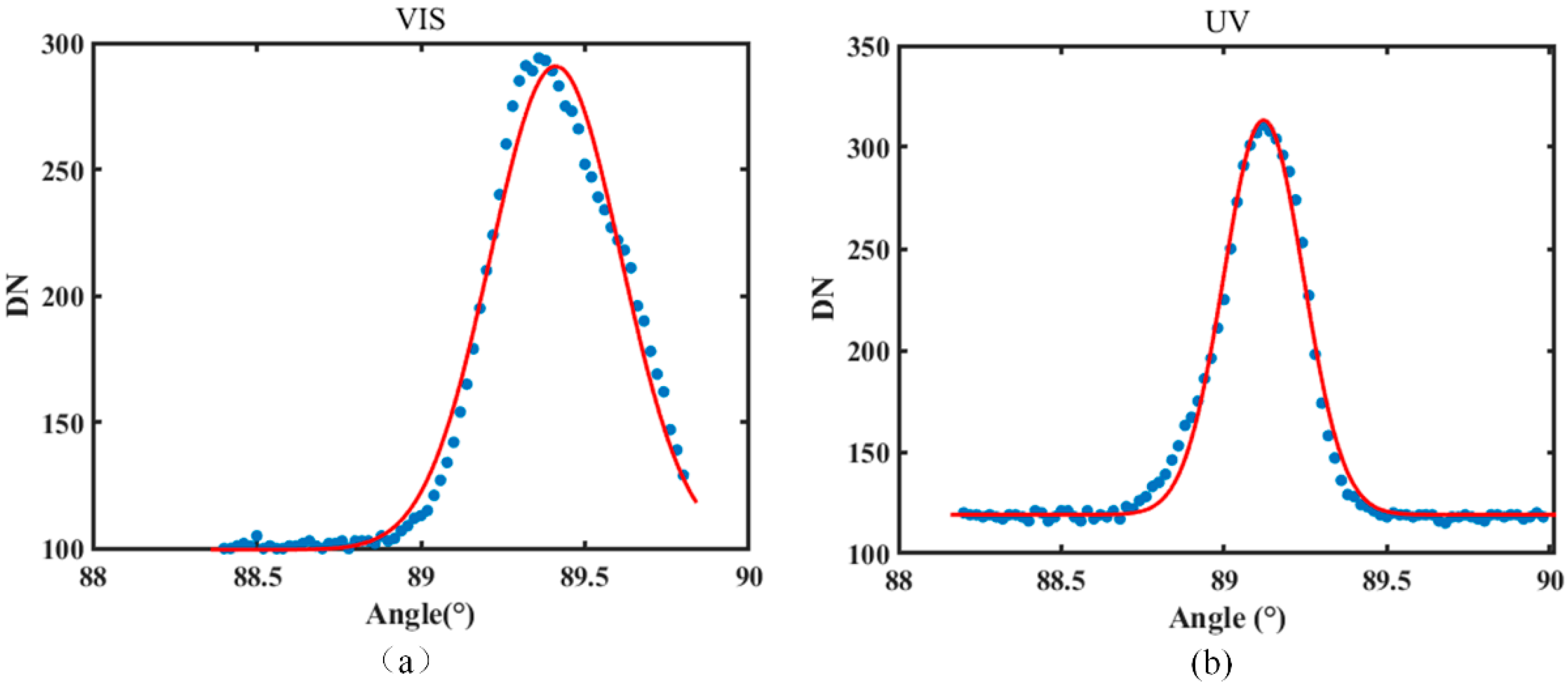
After FOV calibration, the total detection field of view of OMS-N was determined to be 112°, based on the number of pixels in the spatial dimension of the detector. The spatial response function (SRF) defines the angular response of the instrument to incident radiation and is inherently two-dimensional because both azimuth and elevation angles must be considered. The principal direction of the incoming radiation is determined by the centroid (barycenter) of the energy distribution. A collimated white light beam from a 1000 W xenon lamp was directed into the Earth port of the instrument to determine the pixel-level SRF. An alignment cube ensured coaxial alignment of the beam, and the relative orientation of the instrument was determined using a theodolite. For OMS-N, the spatial resolution is defined as the SRF in the cross-orbit direction under nadir observation. During calibration, the rotary table was adjusted in 0.02° increments near the lower edge of the OMS-N field of view. The CCD output was recorded for each pixel along the spatial dimension, and the angular position was fitted to the corresponding pixel digital number (DN) response curve. The FWHM of the fitted Gaussian curve was used to determine the angular spatial resolution (Figure 9).
The horizontal axis in Figure 8 represents the incident angle, with a minimum sampling interval of 0.02°. The vertical axis corresponds to the DN of fixed pixels. The red line represents the Gaussian fitting curve, and the FWHM of this curve defines the spatial resolution. The measured spatial resolutions were 0.478° for the VIS channel and 0.477° for the UV channel, both consistent with the design specifications.
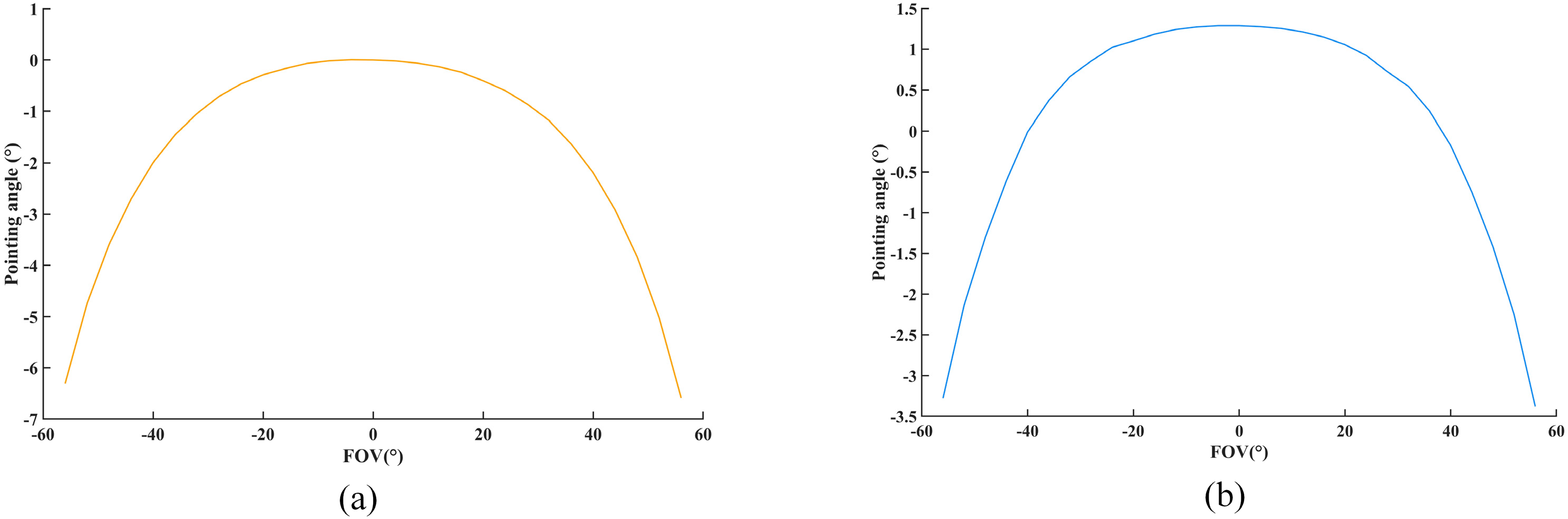
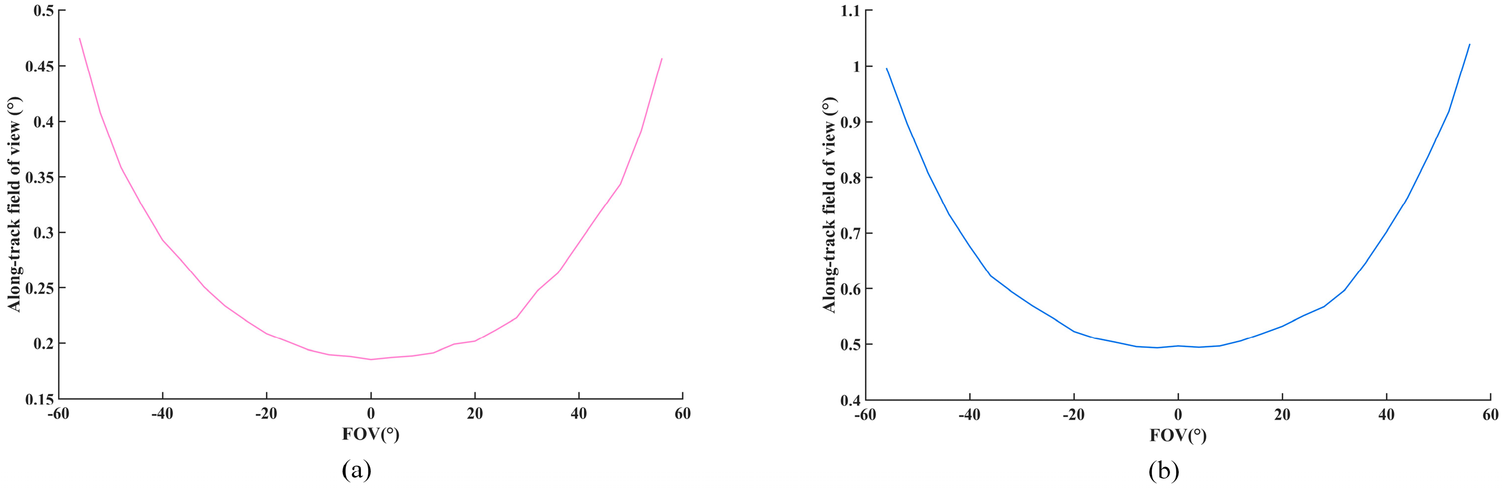
Owing to the optical characteristics of OMS-N, each cross-orbit field-of-view angle corresponds to a distinct geometric pointing angle. The calibration procedure was similar to that used for total field-of-view calibration. The rotary table pitch angle was adjusted in small increments to perform angular scanning (i.e., along the satellite orbital direction). This process established the relationship between pointing angle and field-of-view curve, as well as the correspondence between different field-of-view angles and the along-track FOV angle (Figure 10 and Figure 11).
Figure 10 and Figure 11 illustrate the relationship between FOV and pointing angle for the VIS and UV1/UV2 channels. In these plots, the cross-track field-of-view angles are shown on the horizontal axis, and the along-track pointing angles are shown on the vertical axis (Figure 10). Figure 11 further demonstrates the total along-track FOV, highlighting the variations associated with changes in the viewing angle. The results indicated that the edge along-track FOV was wider than that at nadir, and the corresponding pointing angles were also larger. For both VIS and UV1/UV2 channels, the angular difference between the maximum off-nadir pointing angle and the nadir direction was approximately 1.29°, consistent with the OMS-N optical design.

3.3. Radiometric Calibrations

3.3.1. Dark Signal

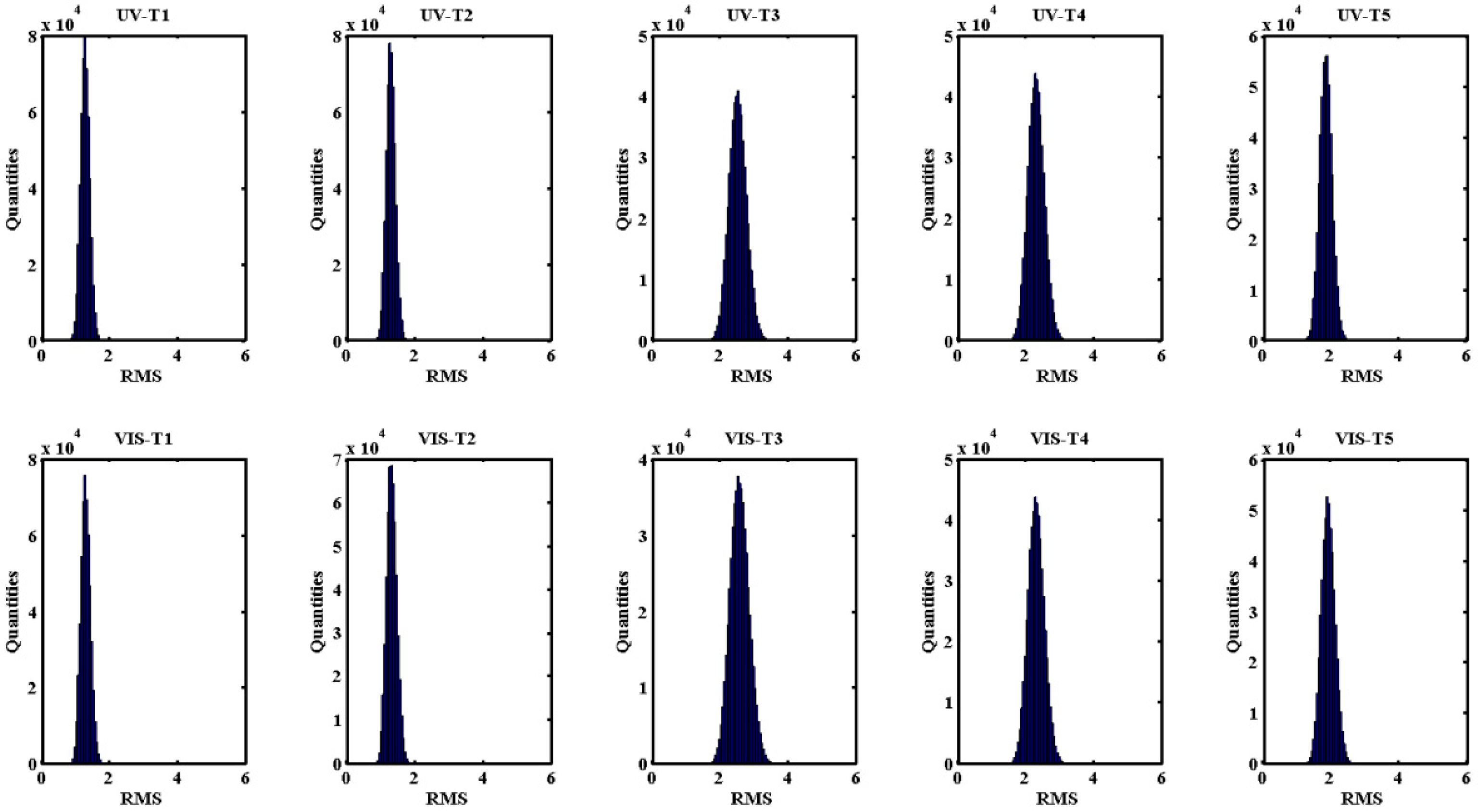
Dark current is a fundamental parameter for evaluating instrument stability. Therefore, dark background calibration was performed prior to radiometric calibration. In addition to pixel-to-pixel variations, detector temperature also affects dark noise. Because the detector temperature was actively controlled during calibration, the dark noise distribution across all pixels followed a normal distribution. The effective exposure time associated with dark noise varied across five different exposure settings, with at least two gain levels being tested for each setting.
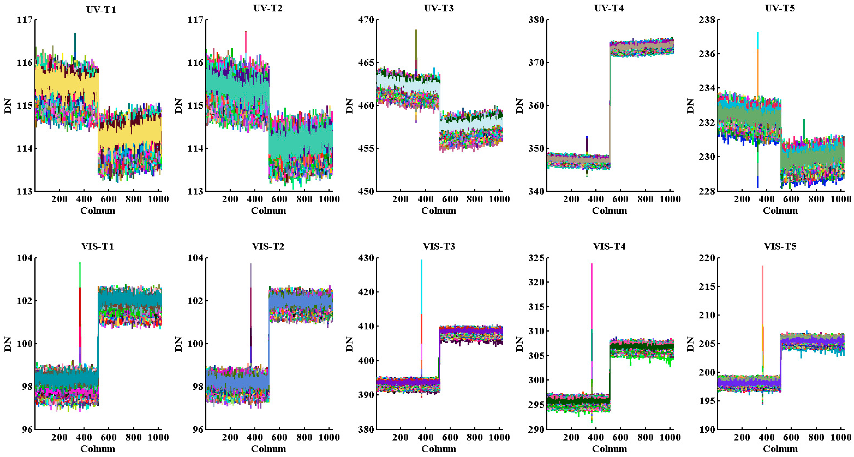
The OMS-N detectors, each with a 512 × 1024 array, were evaluated under non-binning conditions. Figure 12 shows the noise distributions at different integration times, all of which followed a normal distribution. Under non-binning conditions, the grayscale distributions of each row were plotted separately (Figure 13). The results indicate the presence of localized spikes in the distributions, originating from pixel-level noise instability at specific positions. Overall, the noise and dark-field DN values of different pixels remained relatively stable, whereas step-like patterns appeared across the 512 columns owing to bias differences between the two sides of the detectors.
To evaluate the overall instrument performance more accurately, non-binned dark frames were first acquired. To ensure consistency with the on-orbit conditions, the OMS-N instrument was tested under its operational temperature range, covering various integration times and gain levels. The test conditions were fully consistent with actual on-orbit observation scenarios. During on-orbit operations, the corresponding background values under matched conditions (integration time, gain, and operating temperature) were subtracted from the acquired observation data.

3.3.2. Radiometric Gain

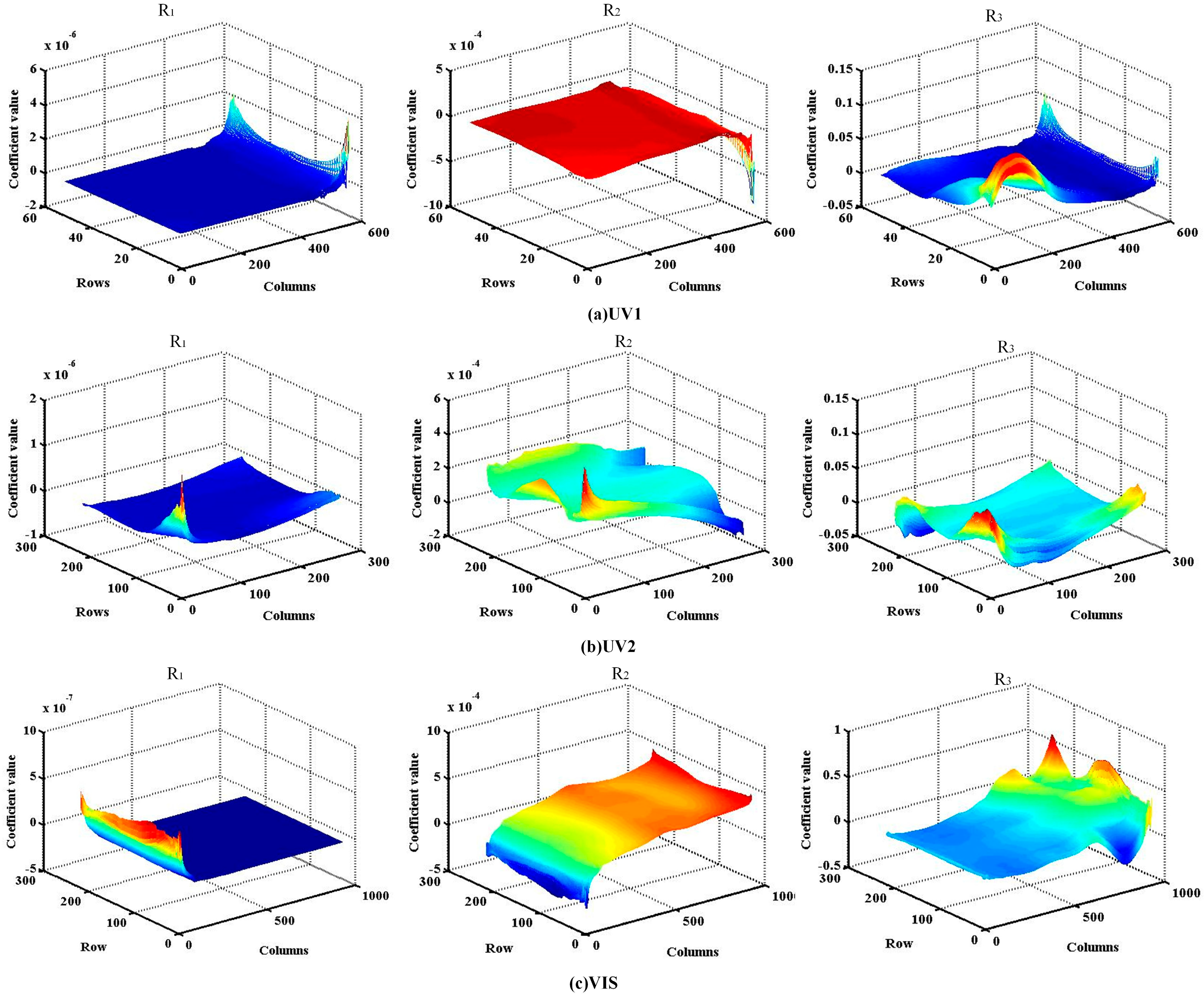
During OMS-N radiance calibration, the emitted radiance was controlled using an integrating sphere as a standard light source. Radiance levels were measured using a radiometer calibrated against a blackbody reference. Radiometric calibration employed different light sources depending on the spectral channel. Xenon lamps were used for the UV1 and UV2 channels, providing strong high-energy emission in the 250–320 nm range. For the VIS channel, tungsten lamps were used, producing a smooth spectral output between 310 and 493 nm but with limited emission below 300 nm. Tungsten lamps also provide a stable broadband output. Six distinct spectral radiance levels (L(i), i = 1, 2, 3, 4, 5, and 6) were generated by controlling the integrating sphere to simulate the nonlinear response of OMS-N. Calibration procedures and data processing methods followed the established approaches [12]. Equation (5) was used to derive the radiometric calibration coefficients, and the fitting results are presented in Figure 14.
L r o w , c o l = R 1 r o w , c o l × D N 2 ( r o w , c o l ) + R 2 r o w , c o l × D N ( r o w , c o l ) + R 3 r o w , c o l
where row and col represent the pixel indices, L ( row , col ) represents the radiance of the pixel (μW/(cm2/sr/nm)), R n (n = 1, 2, 3) represents the radiance responsivity of the pixel, and D N ( row , col ) denotes the signal counts after dark signal subtraction.
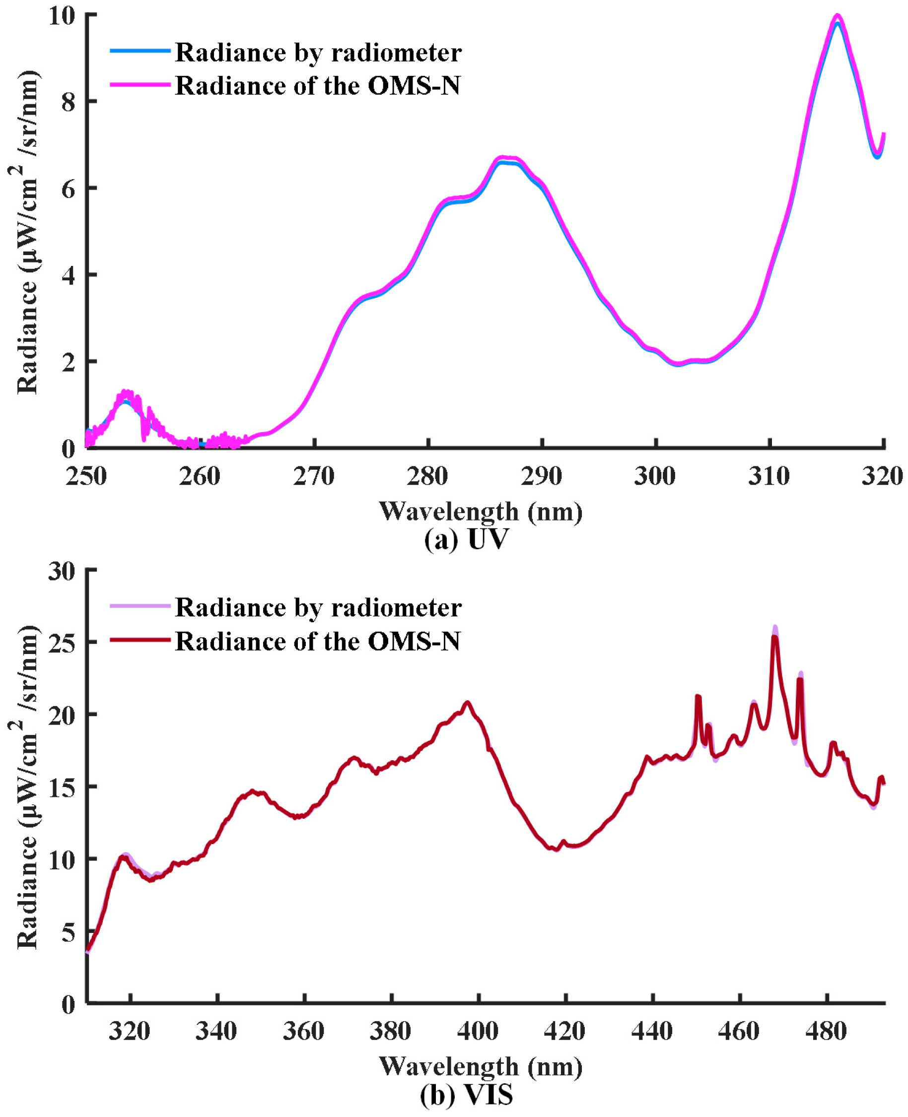
Figure 15 shows the radiance values of OMS-N in the central field of view, along with the corresponding reference radiance values measured by the transfer radiometer.
Radiance values were calculated after background subtraction and application of the calibration coefficients. The relative uncertainties were 1.84% for UV and 1.45% for VIS, A detailed breakdown of radiometric calibration uncertainties is provided in Section 4.2.1, and pixel-level validation results are reported in our previous study [12].

3.3.3. SNR

The SNR of OMS-N was derived from radiance calibration data. For a fixed pixel, noise was estimated from 50 image samples using Equation (6). The SNR under the standard light source of the integrating sphere was then calculated using Equation (7). Finally, the SNR under on-orbit radiance conditions was obtained using the conversion process described in Equation (8).
R M S ( r o w , c o l ) = i = 1 n D N r o w , c o l D N ¯ r o w , c o l 2 n 1
where D N represents the output gray value of that pixel per image, D N ¯ represents the gray value of that pixel after averaging over multiple images, n represents the number of acquisitions, and standard deviation is the noise level of that pixel.
S N R ( r o w , c o l ) = i = 1 n D N ( r o w , c o l ) / n R M S r o w , c o l
where D N represents the dark-background-subtracted signal of the pixel for each image, n represents the number of acquisitions, and standard deviation is the noise level of the pixel.
S N R r e f ( r o w , c o l ) = S N R L ( r o w , c o l ) L r e f ( r o w , c o l ) L ( r o w , c o l )
where S N R r e f represents the signal-to-noise ratio at the reference radiance level, which corresponds to the average radiance of the characteristic on-orbit target, S N R L is the signal-to-noise ratio at the measured radiance level L, L r e f denotes the required radiance for the reference condition (as listed in Table 1), and L is the radiance of the light source.
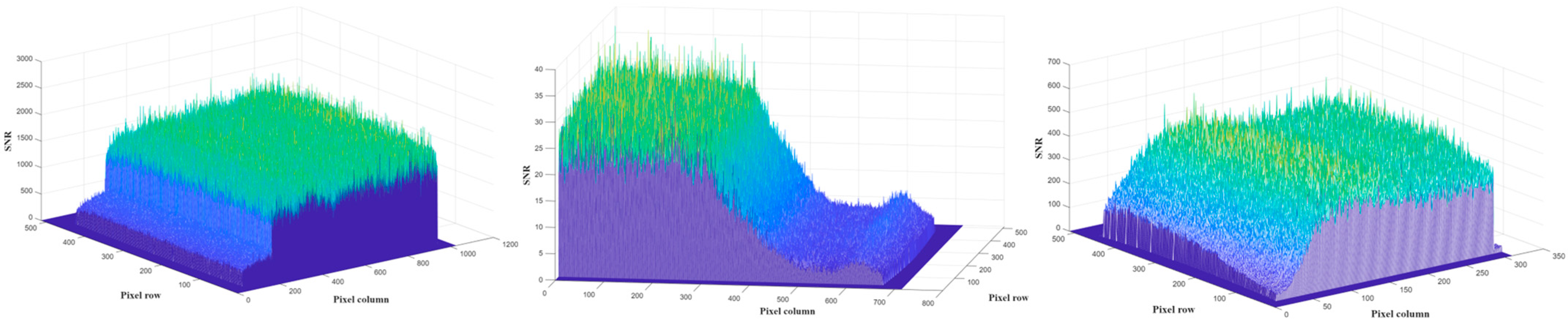
Ground-based calibrated radiance levels often do not reach the levels required for on-orbit UV detection. Therefore, the SNR values were adjusted to reflect the actual average radiance of on-orbit targets. The SNR results for the three OMS-N channels are presented in Figure 16. Because the reference radiance varies across different wavelengths in the VIS channel (as detailed in Table 1), a noticeable decrease was observed in the SNR distribution of the VIS channel. However, the SNR values were sufficient for subsequent retrieval algorithms.
The results demonstrated that OMS-N achieved high SNR across most spectral bands, ensuring reliable data for product retrieval. In particular, performance within the 270–300 nm range provided a robust foundation for ozone profile retrieval.
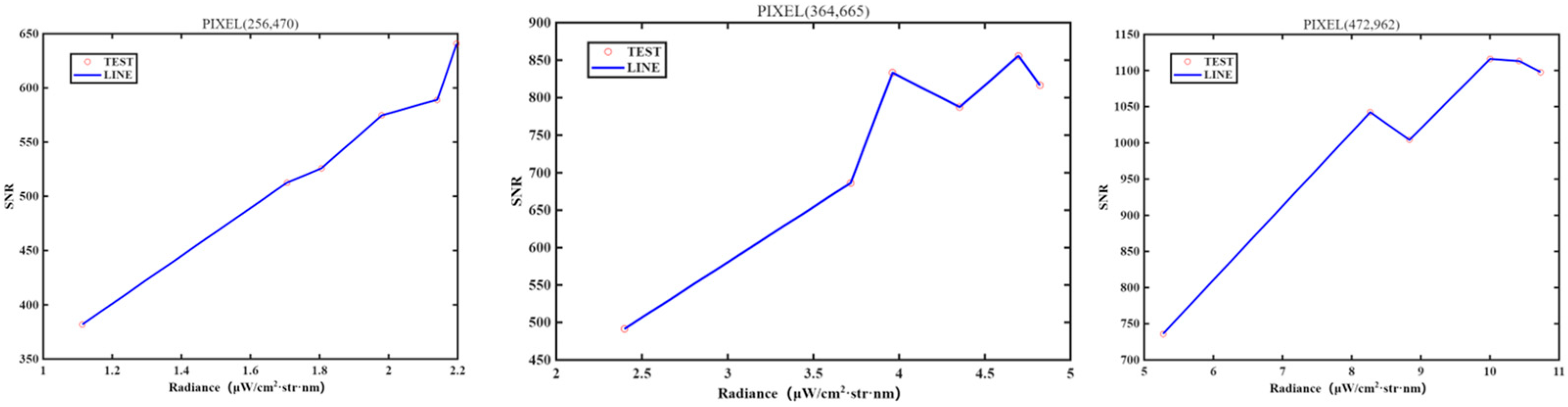
Because target radiance levels may vary significantly during on-orbit observations, a distribution model was developed to describe the relationship between SNR and target radiance. This model was constructed using the multi-level radiometric calibration results presented in Section 3.3.2 and is illustrated in Figure 17.

3.3.4. Sun Diffuser Characterization

The on-orbit calibration system of OMS-N includes solar observation capability. Therefore, the bidirectional reflectance distribution function (BRDF) of the onboard diffuser was calibrated on ground. Accurate measurement of the BRDF distribution characteristics of the diffusers requires assessing the bidirectional reflectance distribution function under varying solar incidence angles (α, β), where α and β represent the angles between the incident sunlight and the satellite flight direction. The sun observation ranges of OMS-N are α ∈ [−4°, +4°] and β ∈ [14.95°, 37.95°]. OMS-N is equipped with two standard diffuser plates (milky white quartz for diffuse scattering), with a calibration cycle of once every 10 days for the calibration plate and once every 3 months for the reference plate.
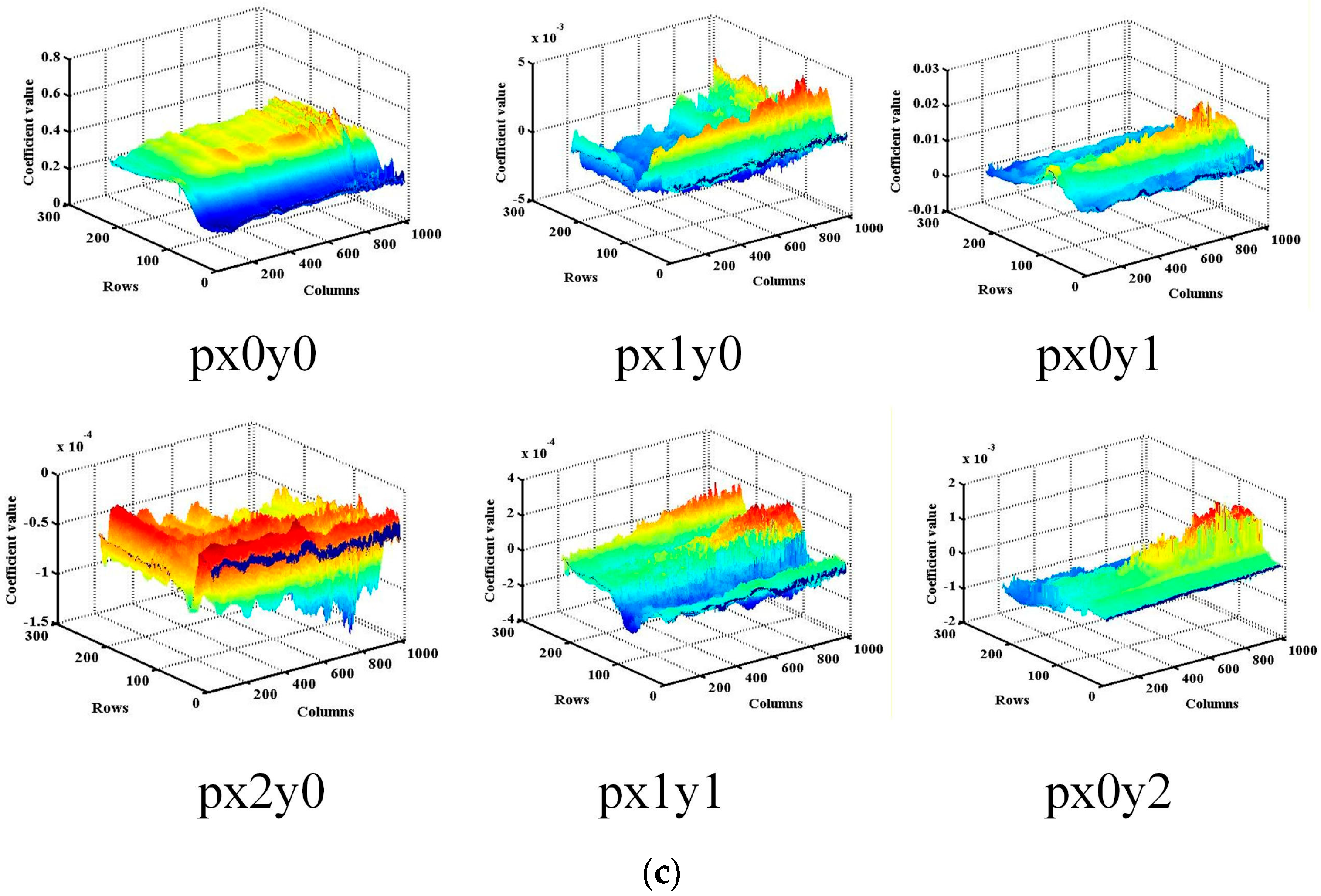
For BRDF calibration, we adopted the standard reference plate transfer method, and the selected reference plate was a polytetrafluoroethylene (PTFE) plate calibrated by NIST. The detection signals in Earth/Sun mode were derived in two steps. First, a solar simulator illuminated the reference diffuser with a known BRDF from a fixed distance L. Second, the instrument was switched to solar mode, where the same simulated light source irradiated the onboard solar-port diffuser at the identical distance L. The conversion relationship between the BRDF of the OMS-N onboard diffuser and that of the reference PTFE plate was then derived by comparing these two sets of detection signals. An “incident angle–DN” dataset was constructed by averaging experimental data obtained under different incidence angles, followed by background subtraction. The radiometric responsivity was calculated for each incidence condition using Equation (9). The NIST-standard diffuser BRDF was converted into an “instrument BRDF” dataset at various incidence angles (Equation (9)). The BRDF is influenced by the diffuser incidence angle, CCD row viewing direction, and CCD column wavelength. The BRDF results for the OMS-N onboard diffuser were obtained at a notional azimuth angle of 26.45° and an elevation angle of 0°. Equation (9) shows the quadratic fitting applied to the “α–β BRDF” dataset. The results indicate a strong dependence of the OMS-N BRDF on both azimuth and elevation angles, which should be considered together with satellite operating conditions. This relationship provides the basis for constructing pixel-level BRDF models [9] across CCD.
BRDF ( row , col ) = px 0 y 0 ( row , col ) + px 1 y 0 ( row , col ) β + px 0 y 1 ( row , col ) α + px 2 y 0 ( row , col ) β 2 + px 1 y 1 ( row , col ) β α + px 0 y 2 ( row , col ) α 2
where px 0 y 0 , px 0 y 1 , px 2 y 0 , px 1 y 1 , and px 0 y 2 are the fitting coefficients; α and β are the incidence angles, with α ∈ [−4°, +4°] and β ∈ [14.95°, 37.95°]; row denotes the row pixel index in the spatial dimension of the detector; and col denotes the column pixel index in the spectral dimension of the detector.
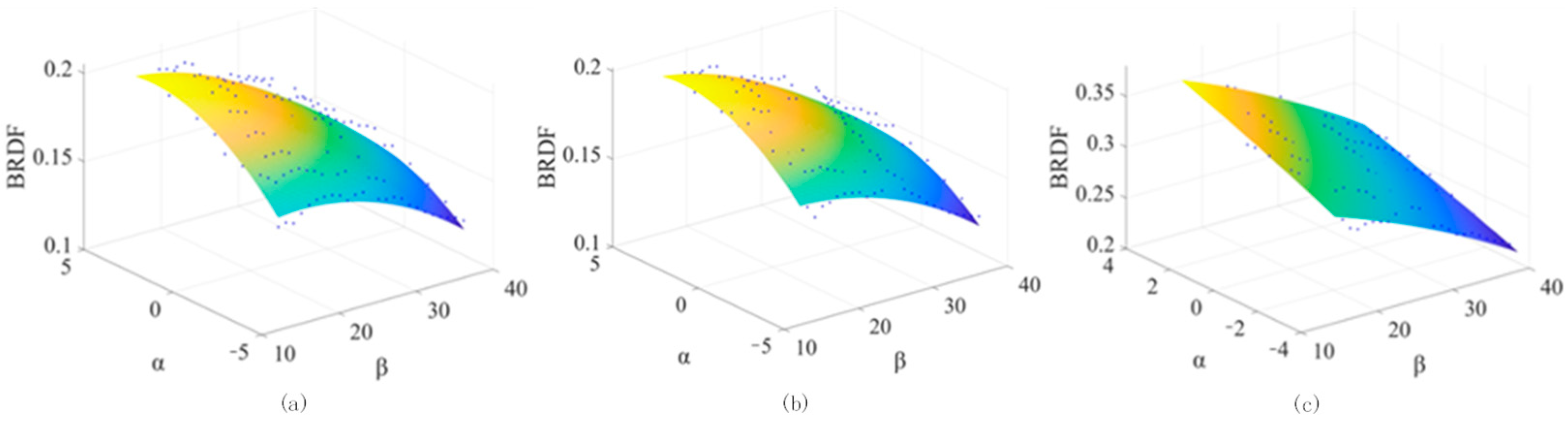
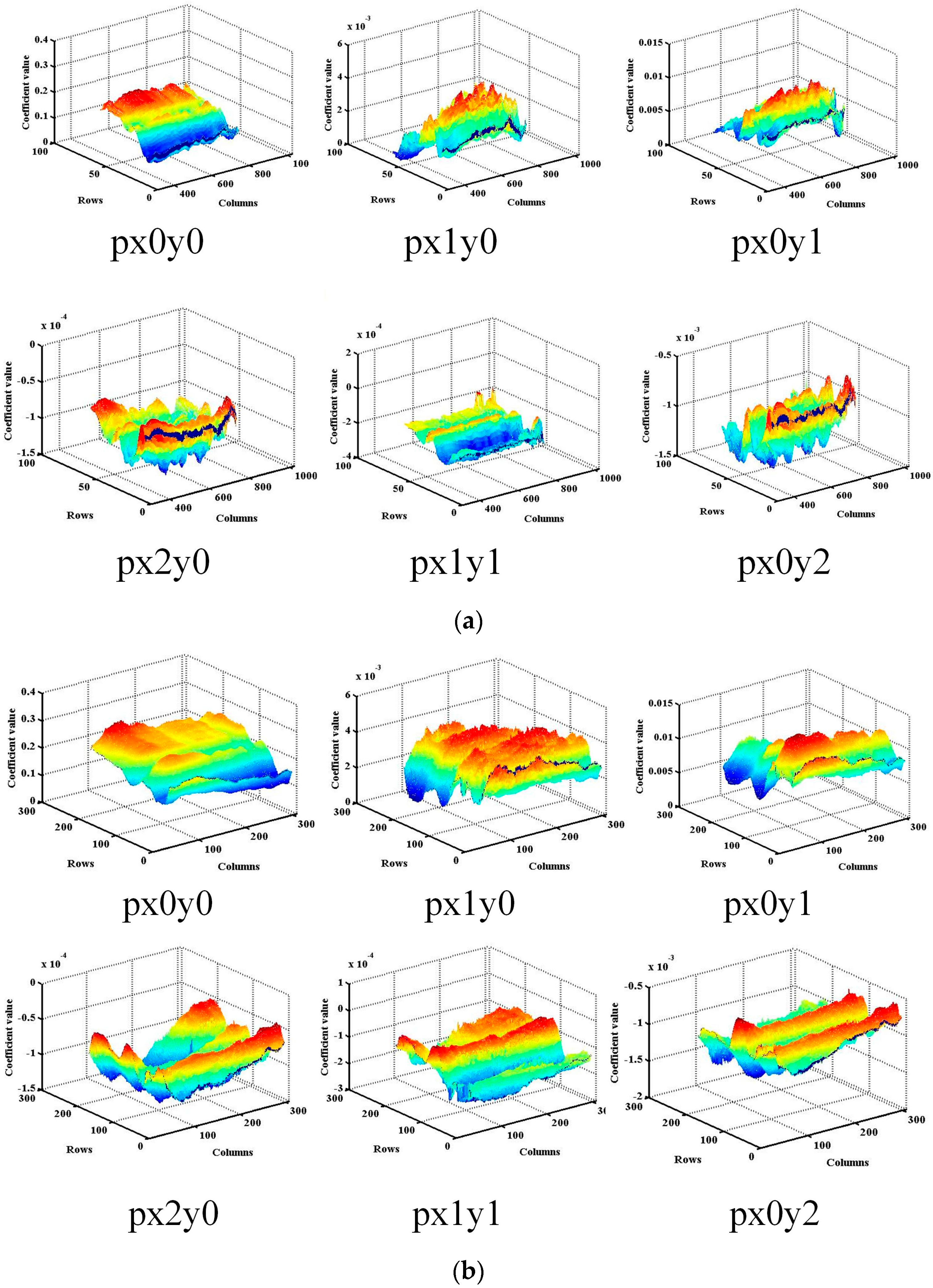
The relationship between the OMS-N diffuser BRDF and variations in α and β angles was described by a fitted surface model. Figure 18 shows the BRDF of diffuser 1 across the UV1, UV2, and VIS channels under varying azimuth and elevation conditions. A quadratic fitting function adequately characterizes the BRDF behavior as a function of azimuth and elevation. The fitted curves for all pixels in both diffusers are shown in Figure 19.

3.4. Nonlinearity and Dynamic Range

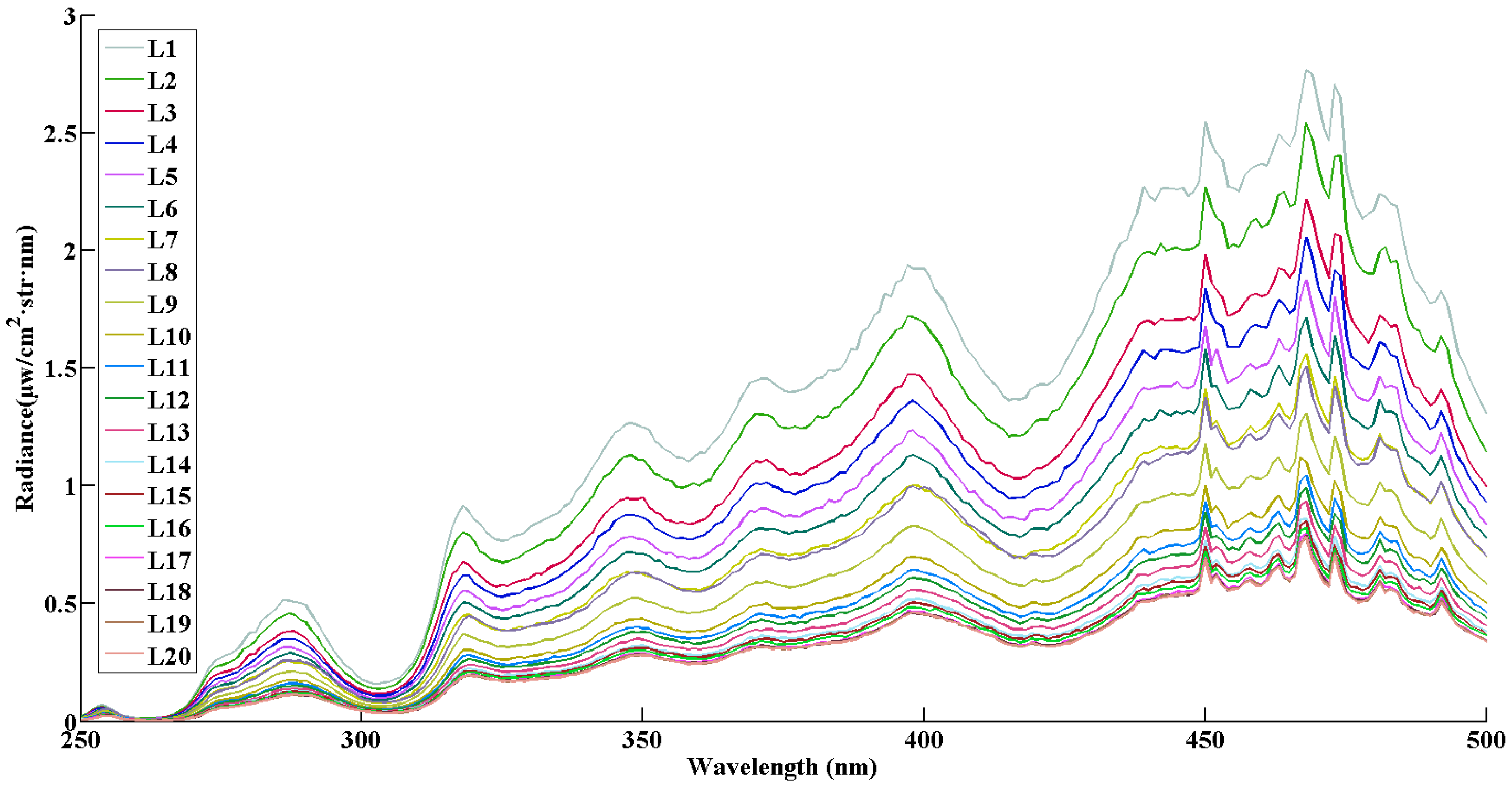
The DN-to-radiance conversion of each CCD output was not strictly linear. Nonlinearity is defined as the deviation between the expected linear response and measured output DN. To assess this behavior, system-level tests were conducted using a xenon integrating sphere as the light source. By adjusting the light-blocking aperture wheel of the integrating sphere and employing a transfer radiometer, a range of light intensities can be continuously varied and introduced into the instrument (Figure 20).
For the same detector, after correcting for nonlinearity, the residual nonlinearity error and full-well DN were found to be consistent across most of the array, with the only exception occurring at UV wavelengths, where low DN values resulted in more pronounced nonlinearity effects. Therefore, linearity was evaluated using the central field of view as a representative case. Twenty different intensity levels were applied until detector saturation was reached. The relationship between input intensity and output DN was then established, and nonlinearity and dynamic range were calculated using Equations (10) and (11), respectively.
dynamic = D N S A T U R A T I O N S D D A R K
NON-LINE = ( D N ( L ) Y F I T ( L ) ) D N ( L )
where dynamic represents the dynamic range expressed in digital numbers, D N S A T U R A T I O N represents the maximum output DN under linear conditions, S D D A R K represents the dark noise, NON-LINE represents the nonlinearity, D N ( L ) is the DN output at a radiometer intensity L, and Y F I T ( L ) is the fitted linear response value at the same radiometer intensity L.
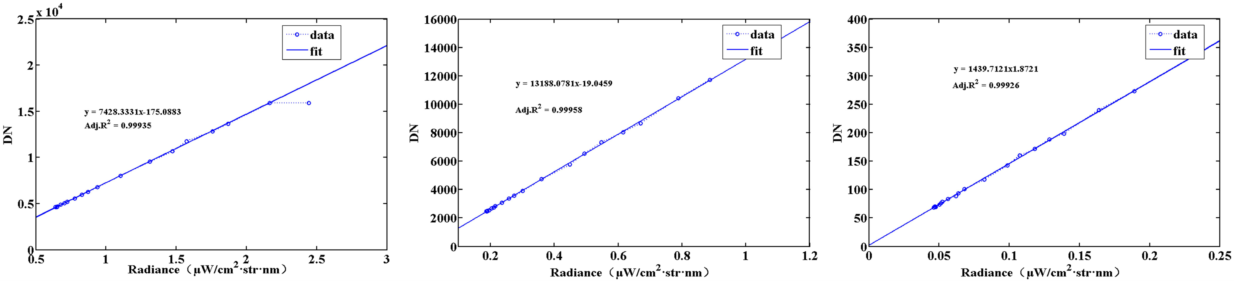
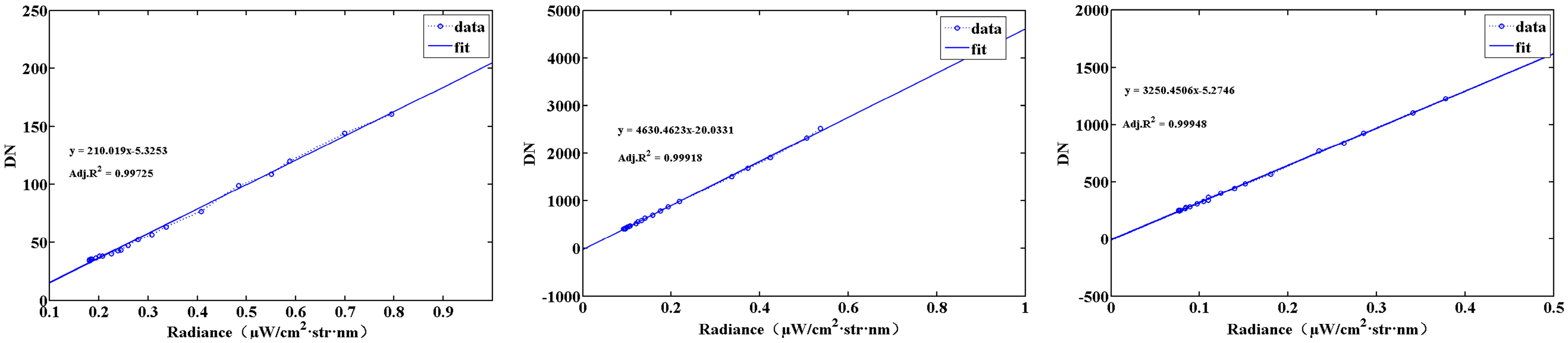
Three pixel positions, (256, 820), (256, 179), and (256, 3), were selected to represent the linear dynamic response curves of the VIS channel in Figure 19. Owing to variations in the spectral intensity distributions across different spectral dimensions, three additional pixel positions, (256, 2), (256, 125), and (256, 572), were selected to represent the linear dynamic response curves of UV1 and UV2 detectors. These positions corresponded to the high-, mid-, and low-radiance regions, respectively. The results indicate that detector nonlinearity was consistent across different radiance levels (Figure 21 and Figure 22).
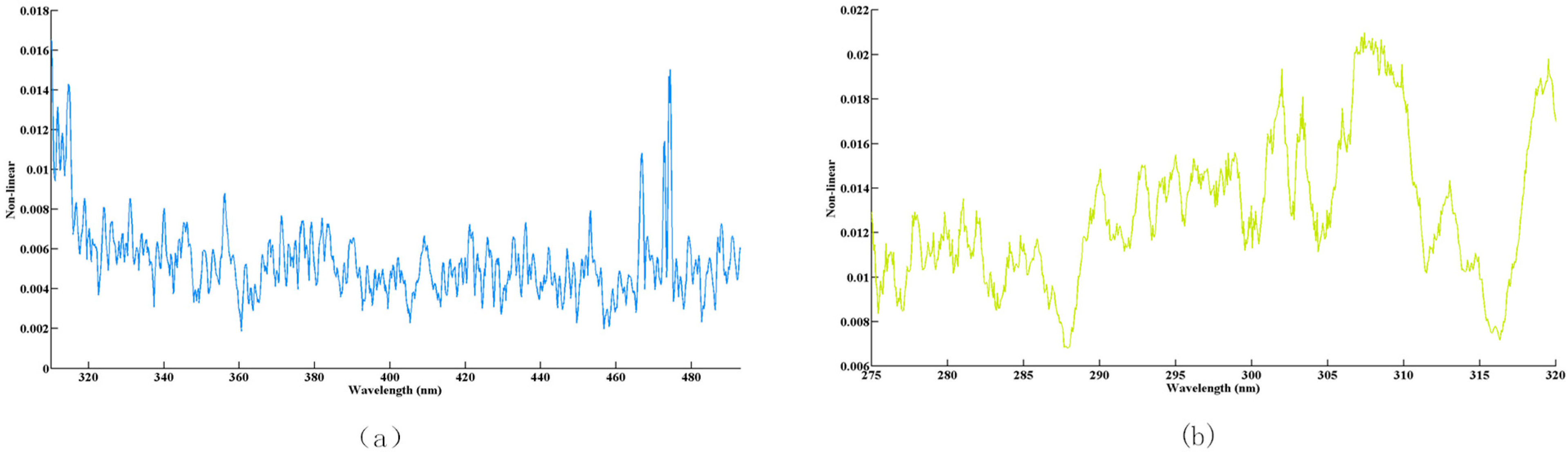
Because the UV1 and UV2 channels received relatively low radiance, saturation could not be achieved in the thermal vacuum chamber. However, these detectors shared the same model and production batch as the VIS channel, and component-level tests confirmed similar linear characteristics and full-well DN. The OMS-N exhibited a full-well DN of 16,383 (16,383 = 214 − 1) and a maximum linear-region DN of 15,989. For the VIS channel, the data points used in the linear fit were applied to Equation (11) across different spectral bands. After excluding the saturation points, the nonlinearity values were averaged, yielding maximum nonlinearities of 1.5% for the VIS channel and 2% for the UV1/UV2 channels (Figure 23). Because the signal-to-noise ratio was lower in the UV1/UV2 bands at 250–275 nm, the calculations were based on wavelengths above 275 nm.

3.5. Polarization Sensitivity

OMS-N is equipped with a spatial depolarizer to mitigate the impact of polarization on the instrument. During performance characterization, the polarization sensitivity of the OMS-N central field of view (FOV) was measured. The test setup employed a uniform light source coupled with a polarizer. By rotating the polarizer, polarized light with varying polarization states was generated, and the OMS-N instrument recorded the corresponding response distribution. The polarization sensitivity was then calculated based on these measurements. Based on the calculations, the average polarization sensitivity of the OMS-N central FOV is 3.3% across the full UV channel spectral range and 4.5% over the entire VIS channel spectral range.

3.6. Straylight

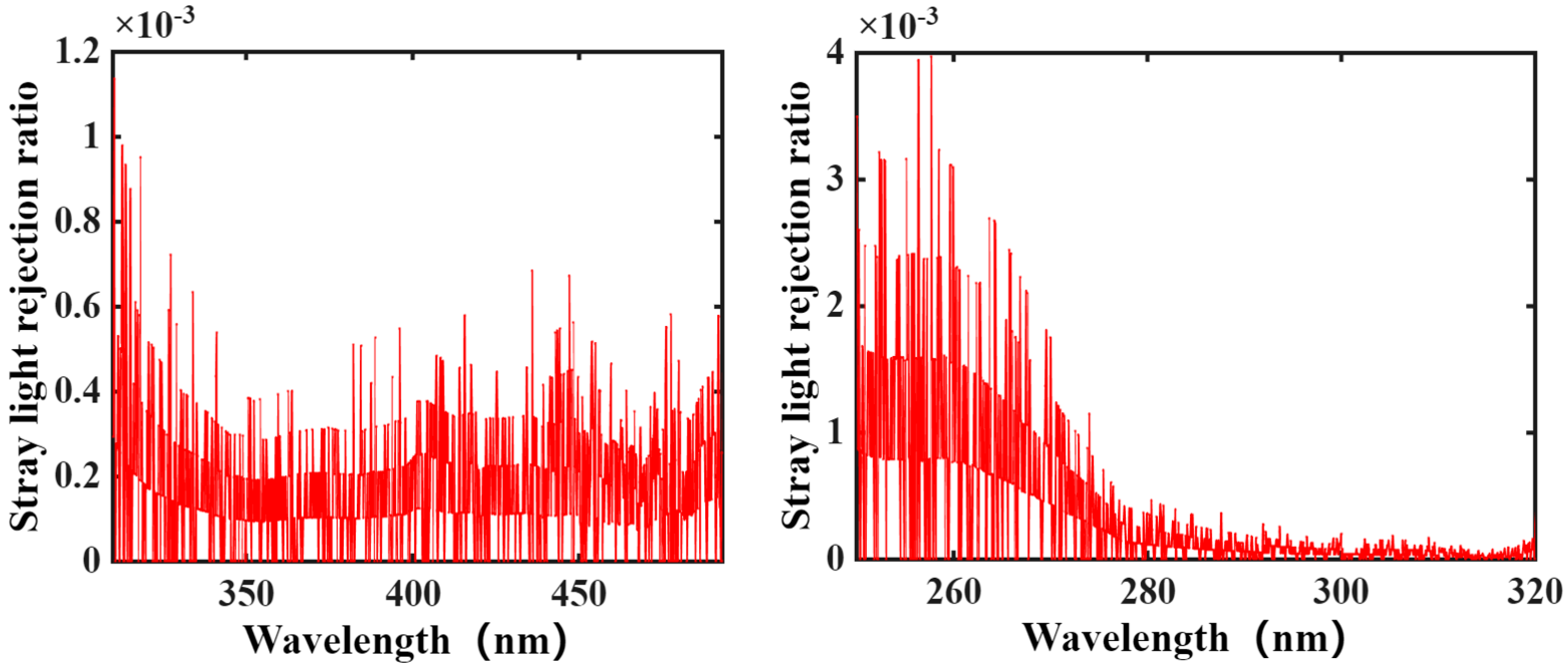
Out-of-band stray light is a key interfering factor that limits the quantitative detection accuracy of hyperspectral imaging payloads. Its primary characterization objective is to quantify the payload’s ability to suppress responses to incident light outside its operating spectral band. In this study, a test scheme based on out-of-band filters was adopted. This method uses optical filters to selectively transmit out-of-band radiation while effectively eliminating in-band signal interference.
The test procedure was as follows. First, out-of-band filters with a high cut-off depth were selected, covering typical spectral regions outside the payload’s operating band (310–495 nm for OMS-N; e.g., the 500–800 nm near-infrared band). The filters were designed to achieve an in-band rejection ratio ≥104 and a transmittance ≥85% at the target out-of-band wavelengths. The filters were then placed between the exit port of the uniform light source and the entrance pupil of OMS-N, with an integrating sphere providing stable and spatially uniform out-of-band illumination.
All tests were performed in a dark-field setting. The dark-field response baseline of the payload was first recorded. Subsequently, different out-of-band filters were introduced sequentially while maintaining consistent incident radiance, and the payload response at each out-of-band wavelength was measured. The out-of-band stray light suppression ratio was derived by calculating the ratio between the out-of-band response and the response under in-band standard radiance, thereby completing the quantitative evaluation of stray light characteristics.
For the stray light performance characterization of OMS-N, testing was focused on the central field of view to evaluate stray light suppression capability in the core detection region. The response characteristics of the central field of view to interfering radiation from different out-of-band regions were systematically obtained, and the results are shown in Figure 24.

4. Discussion

4.1. Pixel-Level Calibration Innovation

The core scientific novelty of this study lies in the establishment of a unified pixel-level calibration framework that integrates both spectral and radiometric calibration for the OMS-N wide-field-of-view (112°) hyperspectral instrument. This framework represents a fundamental departure from conventional channel-level calibration strategies.
For wide-field hyperspectral spectrometers, spatial–spectral distortions such as Spectral Misregistration along the Instrument Line Edge (SMILE) and Keystone effects introduce pronounced pixel-to-pixel variations in the radiometric response. These effects are typically overlooked in traditional channel-averaged calibration methods. Such distortions lead to wavelength shifts, spatial response non-uniformity, and radiometric bias across the detector array, directly degrading the quality of radiance retrievals and subsequent atmospheric trace gas analyses.
In this study, we address these limitations by constructing a pixel-level SRF model for every detector pixel, along with a corresponding pixel-level radiometric calibration model. Unlike channel-level SRF models, which assume a uniform spectral response across all pixels within a spectral channel, the proposed pixel-specific SRF model captures the unique spectral characteristics of each pixel, including central wavelength, full width at half maximum, and amplitude. This enables direct correction of radiometric response differences induced by SMILE and Keystone effects at the individual pixel level. Consequently, the need for post hoc spatial–spectral corrections was eliminated, and systematic biases introduced by channel-averaged approximations were avoided.
By extending pixel-level modeling to both spectral and radiometric calibrations, the reliability and consistency of OMS-N radiance data were significantly improved. This innovation is particularly important for quantitative remote sensing, as precise pixel-level radiance measurements are essential for accurate retrieval of atmospheric trace gases (e.g., O3, NO2, and SO2). These measurements preserve the fine spatial and spectral features required for trace gas detection. To further validate the robustness and quantitative performance of this pixel-level framework, a comprehensive analysis of calibration uncertainty components and their contributions is presented in the following section.

4.2. Calibration Uncertainty

4.2.1. Radiance Calibration Uncertainty

The absolute radiometric uncertainty derived from Equation (12) accounts for transfer radiometer traceability, source uniformity and stability, and instrument instability. The total uncertainty was 2.33% for the UV channels and 1.69% for the VIS channel (Table 3).
δ = x 1 2 + x 2 2 + x 3 2 + x 4 2 + x n 2 × 100 %
where δ denotes the total uncertainty, and xn denotes the uncertainty of each sub-component.
The detailed test procedures for each uncertainty component are as follows.
Transfer Radiometer Uncertainty: The transfer radiometer was calibrated by China’s National Institute of Metrology (NIM) across OMS-N’s full radiance range. The traceability uncertainty of the radiometer listed in the table is actually a combined uncertainty, which includes nonlinearity, instability, and blackbody traceability uncertainty under single-level radiance conditions.
Source Exit Angle Uniformity: The radiance of the extended light source was measured at different exit angles using a transfer radiometer. This uncertainty was derived from the variations in radiance across these angles.
Source Instability: The light source intensity was monitored in real time using a transfer radiometer over a 5 h period. This component was calculated based on temporal intensity fluctuations during the monitoring period.
Source Non-uniformity: The radiance distribution of the extended light source was measured at different spatial positions (under the same exit angle) using a transfer radiometer. This component was determined based on the radiance variation among these positions.
OMS-N Instability: OMS-N was irradiated with a constant light intensity, and the signal was recorded over a 5 h period. This component was calculated as the ratio of the time-domain Standard Deviation (SD) fluctuation to the mean signal value.
R M S E ( r o w , c o l ) = 1 n i = 1 n ( D N i D N ¯ ) 2
where SD(row, col) represents the standard deviation of the detector pixel located at coordinates (row, col), row and col denote the row and column indices of the pixel, respectively; n is the total number of repeated measurements performed on the same pixel; i is the index of each individual measurement, ranging from 1 to n; DNi is the raw digital number output by the pixel in the i measurement; and D N ¯ is the arithmetic mean of all n measured DN values for the pixel.

4.2.2. Irradiance Calibration Uncertainty

The uncertainty associated with the light source itself was negligible because the same source was used in both ground-based calibration and solar-mode calibration, with the same distance maintained relative to the sensor. However, additional sources of error may affect the BRDF calibration of the onboard diffusers. These sources include instrument limitations, alignment errors, environmental variations, and material inconsistencies, all of which can influence reflectance uncertainty and stability as shown in Table 4.
Standard diffuser plate uncertainty: This component is reported in the calibration results from the National Institute of Metrology (NIM) of China and represents the traceable uncertainty of the standard diffuse reflector plate used in the experiments.
Solar simulator distance error: During the irradiance calibration process, this uncertainty component was derived from the distance deviation between the solar simulator and the solar port of OMS-N.
Incident angle error: Based on the Lambertian cosine law and the law of propagation of uncertainty, the relative uncertainty in irradiance introduced by incident angle error is calculated as
u ( E ) E = tan θ u ( θ )
u ( θ ) = Δ θ π 180
where E is Nominal irradiance, u(E) represents the absolute dispersion of irradiance propagated from the incident angle error, θ = 26.45° is the nominal incident angle, and =0.1° is the angle error controlled by the precision rotary stage. After conversion to radians, the calculated relative uncertainty contribution is approximately 0.1% for all channels.
The overall BRDF calibration uncertainty for OMS-N, when assessed on the ground using the described methods, was better than 3%. This residual uncertainty primarily arises from the measurement errors associated with different external light sources.

5. Conclusions

This study presents a systematic pre-launch ground calibration of the Ozone Monitor Suite–Nadir (OMS-N), a payload onboard the FY-3F satellite. Calibration and verification comprehensively covered key parameters, including radiometric calibration, spectral calibration, geometric calibration, nonlinearity, and dynamic range. The absolute radiometric calibration uncertainty of the OMS-N UV1/UV2 channels was better than 2.33%, and that of the VIS channel was better than 1.69%, with a relative uncertainty of ≤1.84%. The spectral wavelength error was ≤0.01 nm for the VIS channel and ≤0.03 nm for the UV1/UV2 channels, and the geometric positioning accuracy was better than 0.1 pixels. In addition, the maximum nonlinearity did not exceed 2%. All performance indicators met or exceeded the design requirements, providing a solid technical foundation for on-orbit quantitative observations.
Based on the accurate parameter models established through ground calibration, OMS-N has successfully performed operational observations in orbit. It has acquired high-quality global data on atmospheric components, including ozone (O3) [13], sulfur dioxide (SO2) [14], nitrogen dioxide (NO2), and aerosols. The stable data output further verified the accuracy and reliability of the pre-launch ground calibration and provided important support for the quantitative assessment of the atmospheric environment.
Considering the potential subtle effects of the on-orbit environment (e.g., ultraviolet stray light and intra-pixel non-uniformity) on instrument performance, on-orbit corrections were applied to OMS-N Level-1 data to further improve data accuracy. In future work, the radiometric response coefficients will be continuously optimized by integrating onboard calibration observations with ground-based synchronous validation results. This effort will provide more reliable input data for the accurate retrieval of Level-2 products, thereby supporting both operational applications and scientific research in atmospheric ozone and trace gas monitoring in China.

Author Contributions

Writing—Original Draft Preparation: J.M.; On-ground Calibration Design: J.M. and Y.W.; Calibration Procedure: J.M., Y.W., P.L., G.D. and Y.Z.; Electronics Design: W.H. and X.L.; Calibration Data-processing Program: J.M. and J.W.; Writing—Review and Editing: Y.W. and J.M.; Data Validation: X.H. and Q.W.; Calibration Coefficient Verification: J.X., F.W. and Z.Z.; Oversight and Management: Y.Y., Q.W., Y.L., W.Z. and X.Z. All authors have read and agreed to the published version of the manuscript.

Funding

This work was supported by the New Generation of Atmospheric Composition Detection Technology [E266000740], the Youth Innovation Promotion Association of the Chinese Academy of Sciences [E2217A06], and the Ultraviolet Hyperspectral Total Ozone Sounder [Y5BZ31AC60].

Data Availability Statement

The data presented in this study are available on request from the author.

Acknowledgments

The authors wish to thank the FY-3F Project team, as well as Zongyao Ou and Guojun Du from the Beijing Institute of Space Mechanics & Electricity (BSME).

Conflicts of Interest

The authors declare no conflicts of interest.

Abbreviations

The following abbreviations are used in this manuscript:
OMS-NOzone Monitor Suite-Nadir
FY-3FFengyun-3F Satellite
UVUltraviolet
VISVisible
UV1Ultraviolet Channel 1
UV2Ultraviolet Channel 2
AODAerosol Optical Depth
NO2Nitrogen Dioxide
ODPSOn-board Data Processing System
RMSERoot Mean Square Error
SDStandard Deviation

References

  1. Veefkind, J.P.; Aben, I.; McMullan, K.; Forster, H.; de Vries, J.; Otter, G.; Claas, J.; Eskes, H.J.; de Haan, J.F.; Kleipool, Q.; et al. TROPOMI on the ESA Sentinel-5 Precursor: A GMES mission for global observations of the atmospheric composition for climate, air quality and ozone layer applications. Remote Sens. Environ. 2012, 120, 70–83. [Google Scholar] [CrossRef]
  2. Levelt, P.F.; van den Oord, G.H.J.; Dobber, M.; Eskes, H.; van Weele, M.; Veefkind, P.; van Oss, R.; Aben, I.; Jongma, R.T.; Landgraf, J.; et al. TROPOMI and TROPI: UV/VIS/NIR/SWIR instruments. In Proceedings of the SPIE OPTICS + PHOTONICS, San Diego, CA, USA, 13–17 August 2006. [Google Scholar] [CrossRef]
  3. Farman, J.C.; Gardiner, B.G.; Shanklin, J.D. Large losses of total ozone in Antarctica reveal seasonal ClOx/NOx interaction. Nature 1985, 315, 207–210. [Google Scholar] [CrossRef]
  4. Zhou, M.Q.; Wang, Y.P.; Robert, C.; Zhang, X.Y.; Zhang, L.; Deng, Z.L.; Qi, C.L.; Wang, P.C. Global carbon monoxide column derived from HIRAS-II/FY-3F satellite observations. Adv. Atmos. Sci. 2025, 42, 1776–1782. [Google Scholar] [CrossRef]
  5. Wang, Z.; Weng, F.Z.; Han, Y.; Hu, H.; Yang, J. Evaluations of microwave sounding instruments onboard FY-3F satellites for tropical cyclone monitoring. Remote Sens. 2024, 16, 4546. [Google Scholar] [CrossRef]
  6. Chen, F.X.; Hu, H.; Weng, F.Z.; Dong, C.J.; Fang, X.; Yang, J. Retrieval of cloud ice water path from FY-3F MWTS and MWHS. Remote Sens. 2025, 17, 1798. [Google Scholar] [CrossRef]
  7. Wang, L.; Chen, S.S.; Hu, X.Q.; Niu, X.H.; Xu, H.L.; Wang, J.W.; Miao, S.X.; Liu, H.; Qi, C.L.; Sun, L.; et al. FY-3F MERSI-III on-orbit calibration methodology and performance of reflective solar bands. IEEE Trans. Geosci. Remote Sens. 2025, 63, 5625815. [Google Scholar] [CrossRef]
  8. Yang, Z.D.; Lu, N.M.; Shi, J.M.; Zhang, P.; Dong, C.H.; Yang, J. Overview of FY-3 payload and ground application system. IEEE Trans. Geosci. Remote Sens. 2012, 50, 4846–4853. [Google Scholar] [CrossRef]
  9. Wang, W.H.; Zhang, X.Y.; Wang, Y.M.; Wang, Y.J.; Zhang, Z.M.; Fu, L.P.; Jiang, F.; Liu, G.Y. Introduction to the FY-3A Total Ozone Unit: Instrument, performance and results. Int. J. Remote Sens. 2011, 32, 4749–4758. [Google Scholar] [CrossRef]
  10. Huang, F.X.; Huang, Y.; Flynn, L.E.; Wang, W.H.; Cao, D.J.; Wang, S.R. Radiometric calibration of the solar backscatter ultraviolet sounder and validation of ozone profile retrievals. IEEE Trans. Geosci. Remote Sens. 2012, 50, 4956–4964. [Google Scholar] [CrossRef]
  11. Jiang, F.; Wang, W.H.; Wang, Y.M.; Wang, Y.J. Calibration in-orbit and retrieval result study of FY-3 Total Ozone Unit (TOU). Chin. J. Geophys. Chin. Ed. 2012, 55, 760–767. (In Chinese) [Google Scholar] [CrossRef]
  12. Mao, J.H.; Wang, Y.M.; Shi, E.T.; Hu, X.Q.; Wang, Q.; Wang, J.D. Pre-launch multi-energy radiance calibration of the OMS-N. Remote Sens. 2024, 16, 119. [Google Scholar] [CrossRef]
  13. Xu, J.; Wang, Y.P.; Chen, L.; Efremenko, D.; Rao, L.L.; Tana, G.; Liu, S.H.; Wang, Q.; Mao, J.H.; Wang, Y.M.; et al. First total ozone column observations from the Ozone Monitoring Suite-Nadir (OMS-N) onboard China’s FengYun-3F satellite. Sci. China Earth Sci. 2025, 68, 3665–3683. [Google Scholar] [CrossRef]
  14. Yan, H.H.; Richter, A.; Zhang, X.Y.; Schönhardt, A.; Visarius, T. Retrieval of SO2 columns from FY3F/OMS instrument observations. EGUsphere, 2025; preprint. [CrossRef]
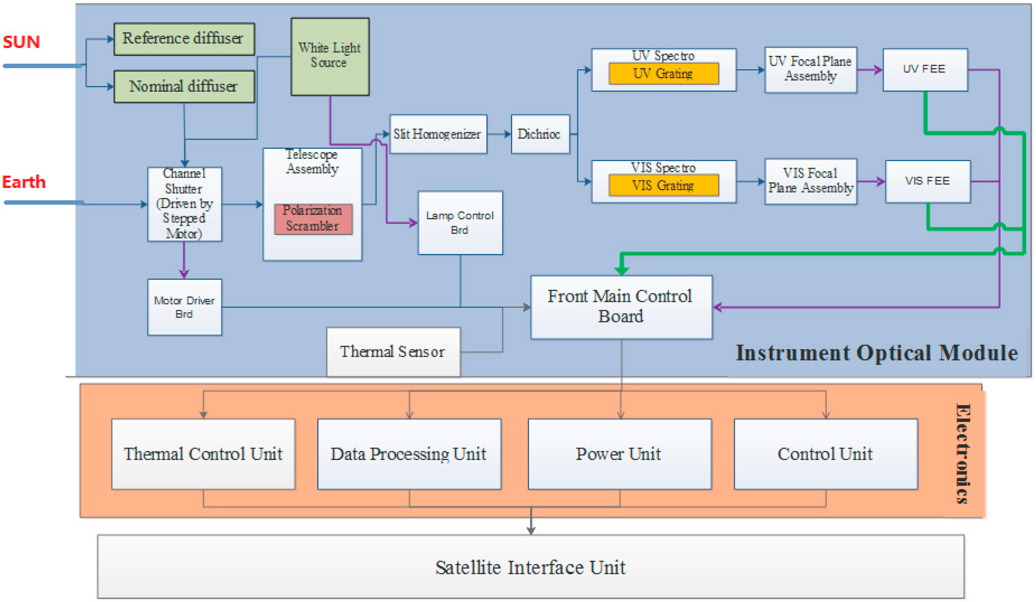
Figure 1. Schematic diagram of OMS-N.
Remotesensing 18 01456 g001
Figure 2. Calibration workflow of OMS-N.
Remotesensing 18 01456 g002
Figure 3. Overview of OMS-N calibration facilities. The OMS-N instrument was mounted on a rotational stage inside the thermal vacuum chamber. The automation control terminal controls the optical ground support equipment, electrical ground support equipment, and rotary table.
Remotesensing 18 01456 g003
Figure 4. Experimental setup for M-square laser calibration.
Remotesensing 18 01456 g004
Figure 5. Wavelength calibration equations for two channels at the initial field of view: (a) VIS channel and (b) UV1 and UV2 channels.
Remotesensing 18 01456 g005
Figure 6. Representative ISRFs of OMS-N for selected pixels. (a) VIS channel and (b) UV channel.
Remotesensing 18 01456 g006
Figure 7. Spatial distribution of spectral resolution for OMS-N: (a) UV1 at 250 nm and (b) VIS at 400 nm.
Remotesensing 18 01456 g007
Figure 8. FOV calibration equations for 309 columns of OMS-N (4 binning). (a) UV1 and UV2 channels and (b) VIS channel.
Remotesensing 18 01456 g008
Figure 9. Spatial resolution of OMS-N for selected fixed pixels. (a) VIS channel and (b) UV1 and UV2 channels.
Remotesensing 18 01456 g009
Figure 10. Relationship between FOV and pointing angle for OMS-N. (a) VIS channel and (b) UV1 and UV2 channels.
Remotesensing 18 01456 g010
Figure 11. Relationship between FOV and along-track field of view for OMS-N. (a) VIS channel and (b) UV1 and UV2 channels.
Remotesensing 18 01456 g011
Figure 12. Dark noise distributions at different integration times for the two detectors.
Remotesensing 18 01456 g012
Figure 13. Mean dark signal distributions across 512 rows under different integration times. Different colored lines represent the individual rows.
Remotesensing 18 01456 g013
Figure 14. Distribution of fitted radiometric calibration coefficients across all pixels. Radiometric responsivity was derived using Equation (5) and integrated DN maps from multiple light sources with known irradiance, with each pixel assigned a unique coefficient (Rn).
Remotesensing 18 01456 g014
Figure 15. Radiance distribution in the central field of view obtained from OMS-N retrievals and reference radiometer measurements.
Remotesensing 18 01456 g015
Figure 16. Distribution of SNR across all pixels. The SNR of OMS-N was calculated using Equations (6) and (7), with the values obtained by converting radiance intensities at different wavelengths under on-orbit conditions. The left, central, and right panels show the results for the VIS (310–493 nm), UV1 (250–300 nm), and UV2 (300–320 nm) channels, respectively.
Remotesensing 18 01456 g016
Figure 17. SNR models for different pixels of OMS-N, with data derived from multi-level radiometric calibration. The curves were fitted to the measured SNR values across varying target radiance levels. During on-orbit operations, the reliability of acquired data can be preliminarily assessed by applying this model to the observed radiance. This model supports the evaluation of on-orbit SNR performance of OMS-N, thereby improving the accuracy, quality, and reliability of retrieved atmospheric data products.
Remotesensing 18 01456 g017
Figure 18. (ac) BRDF of diffuser 1 for the three channels as a function of the azimuthal and elevation angles. (a) Fitted curve for the UV1 channel at 270 nm. (b) Fitted curve for the UV2 channel at 305 nm. (c) Fitted curve for the VIS channel at 350 nm.
Remotesensing 18 01456 g018
Figure 19. (ac) Fitted coefficients for the UV1, UV2, and VIS channels from diffuser 1, each obtained from a set of six fitting coefficients: (a) UV1 channel, (b) UV2 channel, and (c) VIS channel.
Remotesensing 18 01456 g019aRemotesensing 18 01456 g019b
Figure 20. Spectral curves at 20 different intensity levels measured at the exit of the integrating sphere measured using a radiometer.
Remotesensing 18 01456 g020
Figure 21. Linear dynamic test results and fitted curves for three pixel positions of the VIS detector: left (256, 820), center (256, 179), and right (256, 3).
Remotesensing 18 01456 g021
Figure 22. Linear dynamic test results and fitted curves for three pixel positions on the UV detector: left (256, 2), center (256, 125), and right (256, 572).
Remotesensing 18 01456 g022
Figure 23. (a) Nonlinearity of the VIS detector as a function of wavelength. (b) Nonlinearity of the UV detector (UV1 and UV2) as a function of wavelength.
Remotesensing 18 01456 g023
Figure 24. Straylight performance of OMS-N in the central field of view: VIS channel (left) and UV channel (right).
Remotesensing 18 01456 g024
Table 1. Main specifications of OMS-N.
IndexCharacteristics
Scientific ObjectivesO3, SO2, NO2, BrO, O3 profile, Aerosol, and Cloud
ChannelUV1UV2VIS
Spectral range/nm250–300 nm300–320 nm310–495 nm
Spectral resolution/nm~1 nm0.5~0.6
Field of View112°
  Spatial resolution  28 km × 21 km (at nadir)  7 km × 7 km (at nadir)  7 km × 7 km (at nadir)
  SNR  >50@6.4 × 10⁻³ μW/cm2/sr/nm  >200@1.274 μw/cm2/sr/nm  312–340 nm > 200@1.274 μw/cm2/sr/nm
  340–495 nm > 1000@8.0 μw/cm2/sr/nm
  Wavelength calibration accuracy  0.05 nm  0.05 nm  0.05 nm
Table 2. Summary of wavelength calibration deviations.
Theoretical Spectral (nm)OMS-N Spectral (nm)Deviations (nm)
253.652253.62890.0231
334.1484334.1414−0.007
404.657404.6536−0.0034
407.7837407.78790.0042
435.834435.8316−0.0024
Table 3. Absolute uncertainty of OMS-N radiance calibration [12].
ChannelTransfer
Radiometer
Uncertainty
Source Exit
Angle
Uniformity
Source
Instability
Source
Non-Uniformity
OMS-N
Instability
Total
Uncertainty
UV1 + UV22.1%0.2%0.1%@5 h0.9%0.42%2.33%
VIS1.33%0.2%0.1%@5 h0.9%0.47%1.69%
Table 4. Uncertainty components of the diffuser calibration.
ErrorUV1UV2VIS
Source non-uniformity1.5%1.5%1.5%
Standard diffuser plate uncertainty1%1%1%
OMS-N instability0.42%0.42%0.47%
Source instability1%1%1%
Solar simulator distance error0.5%0.5%0.5%
Incident angle error0.1%0.1%0.1%
Total2.165%2.165%2.175%
Disclaimer/Publisher’s Note: The statements, opinions and data contained in all publications are solely those of the individual author(s) and contributor(s) and not of MDPI and/or the editor(s). MDPI and/or the editor(s) disclaim responsibility for any injury to people or property resulting from any ideas, methods, instructions or products referred to in the content.