A Multi-Channel Convolutional Neural Network Model for Detecting Active Landslides Using Multi-Source Fusion Images

Highlights

What are the main findings?

• Based on multi-source fusion images, a new dataset and model were constructed for active landslide detection.
• The model introduces a Landslide Attention Module, which has a significant effect on improving the model’s performance in detecting active landslides.

What are the implications of the main findings?

• The proposed model achieves superior overall performance and generalization.
• Training with multi-source fusion images enhances performance and efficiency while reducing computation and parameters.

Abstract

Synthetic Aperture Radar Interferometry (InSAR) has demonstrated significant advantages in detecting active landslides. The proliferation of computing technology has enabled the combination of InSAR and deep learning, offering an innovative approach to the automation of landslide detection. However, InSAR-based detection faces two persistent challenges: (1) the difficulty in distinguishing active landslides from other deformation phenomena, which leads to high false alarm rates; and (2) insufficient accuracy in delineating precise landslide boundaries due to low image contrast. The incorporation of multi-source data and multi-branch feature extraction networks can alleviate this issue, yet it inevitably increases computational cost and model complexity. To address these issues, this study first constructs a multi-source fusion image dataset combining optical remote sensing imagery, DEM-derived slope information, and InSAR deformation data. Subsequently, it proposes a multi-channel instance segmentation framework named MCLD R-CNN (Multi-Channel Landslide Detection R-CNN). The proposed network is designed to accept multi-channel inputs and integrates a landslide-focused attention mechanism, which enhances the model’s ability to capture landslide-specific features. The experimental findings indicate that the proposed strategy effectively addresses the aforementioned challenges. Moreover, the proposed MCLD R-CNN achieves superior detection accuracy and generalization ability compared to other benchmark models.

1. Introduction

Globally, landslides represent one of the most devastating geological disasters, causing considerable risks to human life, infrastructure, and socio-economic stability annually [1]. As human activities continue to intensify, the occurrence frequency and geographic spread of landslides have progressively escalated, resulting in a significant increase in the associated risks to society [2]. Therefore, conducting high-precision landslide detection and mapping their spatial distribution is of great scientific significance. Furthermore, it is of practical importance for the timely implementation of disaster prevention and mitigation measures, ultimately helping to reduce disaster losses [3,4].

Conventional landslide detection methods have primarily relied on field surveys, offering precise and dependable data regarding landslides [5]. However, this approach is time-consuming, labor-intensive, and costly, rendering it unsuitable for large-scale landslide mapping [6]. In contrast, remote sensing technology, known for its extensive spatial coverage and high detection efficiency, has demonstrated significant promise in landslide detection and is extensively used in geological hazard monitoring. For instance, the integration of optical remote sensing and Light Detection and Ranging (LiDAR) techniques has significantly improved landslide detection efficiency [7,8,9]. Nevertheless, both optical imagery and LiDAR mainly rely on changes in surface morphology or structural features. Consequently, they are effective only for detecting landslides that exhibit substantial surface displacement. Their capability to identify active landslides with slow movements but without noticeable surface changes remains limited. These undetected active landslides may pose potential long-term threats to local residents and infrastructure. Recently, Interferometric Synthetic Aperture Radar (InSAR) technology has advanced significantly. Through interferometric processing of multi-temporal SAR images collected from the same region, InSAR can precisely extract high-resolution data on surface topography and deformation [10,11,12,13,14]. Given InSAR’s capability to detect millimeter-level ground displacement, it possesses inherent advantages in identifying active landslides [15]. Compared with other techniques, InSAR provides all-weather, day-and-night, and high-precision monitoring capabilities [16,17], and has thus been extensively applied in active landslide detection studies [18,19,20,21]. However, large-scale InSAR-based active landslide detection still faces major challenges due to a lack of efficient, automated interpretation methods. Processing massive interferometric datasets remains computationally complex and heavily dependent on manual intervention. Consequently, the establishment of an automated and large-scale detection framework based on InSAR has emerged as an important research hotspot in recent years.

Driven by the rapid progress of computing technology, deep learning has evolved rapidly, offering an innovative approach for achieving automated landslide detection [22,23,24]. Several studies have combined optical remote sensing imagery and DEM-derived information [25,26] with deep learning architectures, including object detection, semantic, and instance segmentation networks [27], enabling the automatic identification of landslides [28,29]. Building on these technological advances, numerous studies have investigated the fusion of InSAR observations with deep learning techniques to achieve large-scale automated identification of active landslides. For instance, integrating InSAR-derived deformation maps with networks like Faster R-CNN and Yolo enables the efficient recognition of active landslide distributions. This effectively achieves automated detection at a regional scale [30,31,32]. Furthermore, deep learning models based on semantic segmentation, such as U-Net, can extract semantic features of landslides from InSAR deformation fields. This capability enables precise delineation of landslide boundaries and accurate characterization of their spatial extent [33,34]. This approach effectively represents the geographic location and influence zones of active landslides. In summary, the integration of InSAR and deep learning has not only yielded remarkable success in large-scale automated detection of active landslides [35] but also demonstrates considerable promise in improving both the precision and efficiency of landslide detection.

InSAR is capable of detecting various types of slow ground deformation. However, relying solely on a single InSAR product often introduces uncertainties and potential misclassifications in landslide detection. Specifically, large-scale InSAR-based detection faces two critical bottlenecks. First, relying solely on deformation information often leads to high false alarm rates, as non-landslide geological activities frequently exhibit deformation signatures similar to active landslides. Second, accurately delineating landslide boundaries remains difficult, as deformation maps often lack the textural detail required to define precise edges, resulting in coarse segmentation. To improve the robustness of detection outcomes, several studies have developed training datasets through the fusion of various InSAR-derived products, which strengthens deep learning models in capturing the distinctive characteristics of active landslides [35]. Although such approaches have achieved certain improvements in detection performance, they remain limited in distinguishing other geological activities that exhibit deformation patterns similar to those of landslides. Integrating multi-source data is widely considered an effective strategy to address this issue. This strategy involves synergistically combining InSAR deformation measurements, optical remote sensing imagery, and DEM-derived products. Such integration enables the effective differentiation of active landslides from other ground deformations, thereby significantly enhancing detection accuracy and robustness. Several studies have utilized multi-source datasets within deep learning models featuring multi-branch architectures. These approaches have achieved high-precision automated detection of active landslides [25,36]. Nevertheless, these models are typically complex and computationally intensive, often featuring large numbers of parameters. This results in low training efficiency and limits their applicability for large-scale active landslide detection.

To address the aforementioned limitations, this study integrates optical remote sensing imagery, DEM-derived slope data, and InSAR deformation information to construct a multi-source fusion image dataset for active landslide detection. Building upon this foundation, a single-branch multi-channel convolutional neural network (CNN) is developed to enable efficient and automated detection of active landslides, while accurately outlining their spatial extents. The general framework of the research is presented in Figure 1, and the primary aims of this study are summarized as follows:

(1)

To develop a comprehensive dataset for active landslide detection by fusing optical remote sensing imagery, DEM- derived slope information, and InSAR-derived deformation data, with the goal of improving detection accuracy and reliability. The constructed dataset contains multi-source fusion images across multiple spatial scales, which enhances the model’s ability to generalize in detecting active landslides of diverse sizes.

(2)

To propose an active landslide detection model, namely MCLD R-CNN, which supports multi-channel data input and incorporates a Landslide Attention Module to fully exploit the characteristic features of active landslides embedded in the dataset.

(3)

To comprehensively assess how multi-source data influence model performance by contrasting the proposed method with traditional deep learning frameworks and various dataset types, and to further examine the strengths and weaknesses of the model regarding detection accuracy and computational efficiency.

2. Research Area and Data Sources

2.1. Research Area

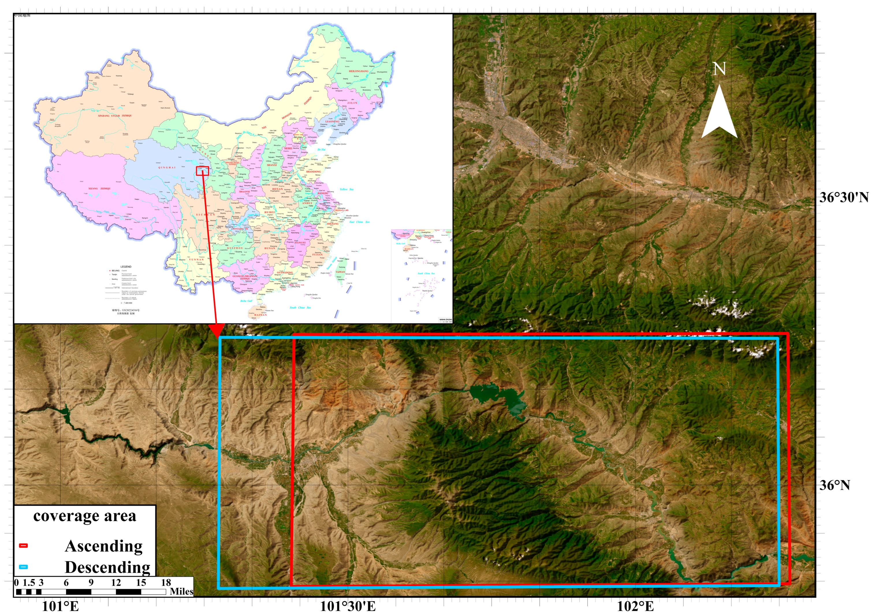
The research region is situated in the upper reaches of the Yellow River within Qinghai Province, China (Figure 2). This region encompasses two major geomorphic terraces in China and functions as a transitional zone between the highly uplifted Tibetan Plateau and the comparatively lower Loess Plateau [37]. Due to prolonged northward compression from the Tibetan Plateau, the region has developed a landscape of mountains and basins. Additionally, erosion from the Yellow River and its tributaries has generated geomorphic conditions conducive to landslide formation [38,39]. The region exhibits an arid to semi-arid continental plateau climate, with most of the 316–436 mm annual precipitation falling in summer and autumn. The unique climate and precipitation characteristics contribute to rock weathering and sparse vegetation, further promoting landslide occurrences [40]. Collectively, these factors contribute to the frequent occurrence of geological hazards, including landslides, which are typically large in scale, widely distributed, formed through complex mechanisms, and possess significant destructive potential [41]. Consequently, these landslide activities provide abundant experimental data for this study and serve as an ideal setting for validating the effectiveness of the multi-source fusion image-based active landslide detection method.

2.2. Data Sources

A total of 165 Sentinel-1 SLC images spanning the research region between 2021 and 2023 were selected, as illustrated in Figure 2. As presented in

Table 1. Fundamental Specifications of the Utilized Sentinel-1 Imagery.

Beam Modes	Polarizations	Flight Directions	Path	Frame	Number of Images
IW	VV + VH	ASCENDING	128	114	45
IW	VV + VH	DESCENDING	33	472	63
IW	VV + VH	DESCENDING	135	473	57

, the satellite data were collected in IW swath mode featuring HH + VH polarization. The images are divided into 45 ascending tracks and 120 descending track datasets. The ascending track data is located at path 128, frame 114, while the descending track data is located at path 33, frame 472, and path 135, frame 473. High-resolution DEMs obtained from ALOS PALSAR, SRTM datasets, and optical imagery sourced from Google Earth that encompass the study region were also acquired concurrently. The SRTM DEM served as auxiliary data for InSAR processing, whereas the SLC imagery, ALOS-derived DEM, and optical data were integrated to construct a multi-source fusion image dataset aimed at detecting active landslides.

3. Method

3.1. Data Preparation and Preprocessing

3.1.1. Initial Data Processing

This study utilized the SBAS-InSAR [42] approach, implemented via the GAMMA software (version 2017) suite [43], to process multiple sets of ascending and descending Sentinel-1 SAR data, thereby deriving the temporal ground deformation rates across the study region. The processing workflow proceeded as follows: First, temporal and spatial baseline thresholds were established (temporal baseline ≤ 36 days, perpendicular baseline ≤ 200 m) to filter valid interferometric pairs, ensuring the continuity and spatial correlation of the time series. Subsequently, differential processing was performed for each pair with a multi-looking factor of 5 (range) by 1 (azimuth), and high-coherence regions (coherence > 0.3) were selected for phase unwrapping using the Minimum Cost Flow (MCF) algorithm. Then, the Singular Value Decomposition (SVD) method was utilized to solve the SBAS linear equations. Subsequently, spatio-temporal filtering was applied to eliminate or mitigate atmospheric disturbances, residual orbital errors, and noise. Specifically, a spatial low-pass filter with a window size of 256 pixels was applied to estimate and remove the spatially correlated atmospheric phase components. In addition, a temporal filter with a window of 70 days was employed to further reduce temporal noise. This process ultimately yielded high-accuracy surface deformation velocities. Finally, the data were transformed from the radar coordinate system to the WGS84 geographic coordinate system, generating final deformation velocity maps in GeoTIFF format. It is important to note that the deformation results from ascending and descending tracks were maintained as independent Line-of-Sight (LOS) velocity maps for subsequent analysis, rather than being decomposed into vector components. The selection of SBAS-InSAR is justified by its superior monitoring accuracy compared to D-InSAR [44]. Furthermore, unlike PS-InSAR, the SBAS method effectively mitigates interferometric decorrelation, rendering it more suitable for detecting active landslides and characterizing their displacement rates [20,45].

In addition, since the study area covers a large region, multiple ALOS PALSAR scenes were utilized to generate the DEM data. Accordingly, the DEM raster tiles were first mosaicked and merged to produce a continuous elevation surface. The topographic gradient was then calculated to extract slope information. This processed slope map served as the topographic input feature for subsequent multi-source data fusion.

3.1.2. Multi-Source Data Fusion

First, the deformation velocity map, slope map, and Google Earth optical imagery were all projected into the WGS84 geographic coordinate system. Based on their spatial reference information, precise image registration was performed among the three datasets to ensure spatial consistency and the reliability of the multi-source fusion results.

To construct a four-channel input tensor incorporating deformation, texture, and topographic features, we adopted a step-by-step fusion strategy. First, the raw InSAR deformation rate data, denoted as V_raw (unit: mm/year), is processed. To suppress the impact of extreme outliers and conform the data to the image format, the deformation rates are clipped within the range [v_min, v_max] (set to −100 and 100 mm/year in this study) and linearly normalized to obtain V_norm ∈ [0, 1] using the following equation:

$$V_{norm}={\displaystyle \frac{clip(V_{raw},v_{min},v_{max})-v_{min}}{v_{max}-v_{min}}}$$

(1)

Subsequently, a pseudo-color mapping function is applied to convert the normalized single-channel data into a three-channel RGB deformation image:

$$C_{def}=\mathsf{\Phi }(V_{norm})$$

(2)

In the formula, $\mathsf{\Phi }$ is a pseudo-color mapping function, where C_def consists of three components: R_def, G_def, B_def.

Following the generation of the deformation image, to highlight deformation characteristics while preserving surface textures, the optical remote sensing image (C_opt) is fused with C_def through a pixel-wise weighted combination. The fused RGB image, C_fused, is calculated as:

$${\mathrm{C}}_{fused}=\lambda \times C_{def}+(1-\lambda )\times C_{opt},\lambda \in [0,1]$$

(3)

In the formula, λ represents the fusion weight coefficient. C _fused is the two-source fusion image, C _def is the deformation rate image, and C _opt is the optical remote sensing image.

Finally, to incorporate topographic features, slope data is embedded as the fourth channel (the Alpha channel) of the image. Let S denote the slope value (in degrees) derived from the DEM. We map the slope range of 0° to 90° linearly to the integer range of 0 to 255 to generate the Alpha channel value A:

$$A=round({\displaystyle \frac{S}{90}}\times 255)$$

(4)

The normalized slope map A is then concatenated with the fused RGB image C _fused to generate the final four-channel input. In this configuration, the normalized slope values serve as the Alpha channel (spanning from 0 to 255), effectively acting as a transparency mask. This linear mapping naturally enhances feature distinctiveness. Specifically, regions with high slopes are rendered with higher opacity to highlight terrain undulations. Conversely, low-slope areas remain more transparent to prioritize the underlying deformation features. Consequently, the resulting four-channel multi-source fusion image efficiently integrates deformation, optical, and topographic information within a single tensor. This approach not only enriches the input features but also enhances both the training efficiency and processing speed of the developed model. The complete data fusion process is depicted in Figure 3.

3.2. Dataset Creation

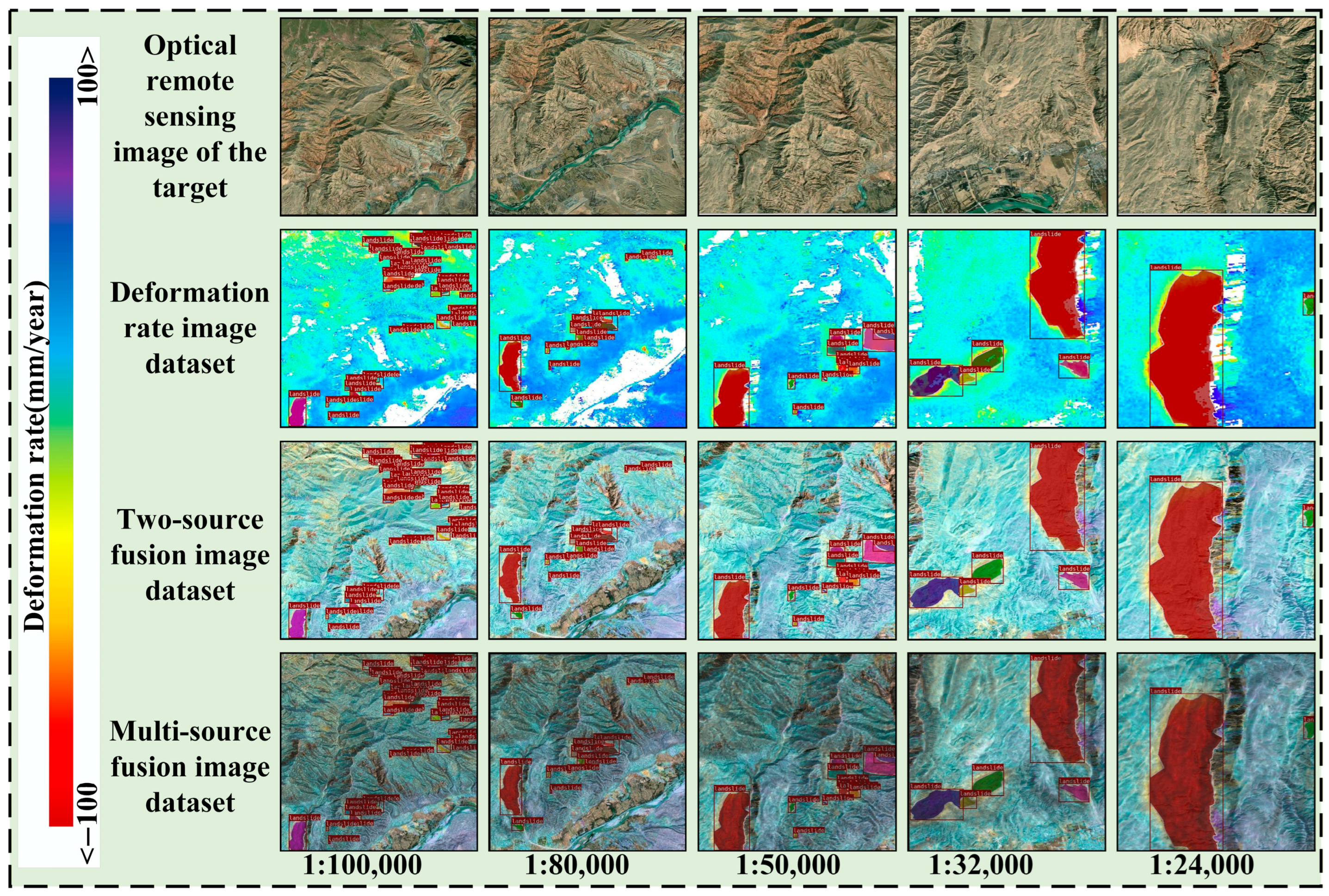
To augment the model’s generalization capability for landslides of varying sizes, this research constructed the dataset using multi-source fusion images at five distinct spatial scales, spanning from 1:24,000 to 1:100,000. The imagery was divided into training tiles with a resolution of 512 × 512 pixels. To ensure the validity and robustness of the dataset, this study established an operational definition for “active landslides” that prioritizes InSAR observation while using optical data for auxiliary verification. Considering that slow-moving landslides [35] (typical velocities less than 1.6 m/year) often lack significant surface changes visible in optical imagery, we primarily identified “activity” based on SBAS-InSAR results. Specifically, areas exhibiting continuous ground deformation with an absolute annual velocity exceeding 10 mm/year [46,47] were classified as active candidates.

Building on this definition, active landslide samples were determined by combining existing landslide data [38,41], optical remote sensing imagery and InSAR deformation information. Quantitative statistics based on spatial overlap analysis reveal that approximately 60% of the labeled samples originated from existing inventories and were subsequently refined using InSAR deformation boundaries. The remaining 40% were newly detected primarily through InSAR evidence, characterized by distinct deformation signals in areas previously unmapped or lacking clear optical signs. Existing inventories functioned as spatial priors; however, it is important to note that we did not directly inherit the boundaries from historical records; instead, all targets were re-verified, and their contours were rigorously re-delineated based on the current InSAR deformation fields. Furthermore, considering the spatial resolution of Sentinel-1 data and the reliability of feature extraction, we set the minimum mapping area to 1000 m². Deformation areas smaller than this scale were excluded from the repository.

As presented in Figure 4, a total of 437 active landslides were detected from the ascending track imagery and 427 from the descending track imagery. To characterize the dataset and assess potential biases, we analyzed the statistical distribution of the labeled active landslides. The landslide areas exhibit a wide range, spanning from a minimum of 1070 m² to a maximum of approximately 6.08 km², with the vast majority concentrated between 2000 m² and 60,000 m². Topographically, the landslides are predominantly located on slopes ranging from 15° to 40°, which aligns with regional landslide susceptibility characteristics reported in [41]. In terms of aspect, the distribution shows a clear preference for east- and south-facing slopes, likely attributable to local microclimatic conditions.

Image augmentation techniques were applied to the sliced images for data expansion. The LabelMe tool was used to manually label the active landslides in the images in COCO dataset format [48]. Following data filtering, the finalized active landslide detection dataset comprised 3450 samples, of which 3105 were allocated for model training and 345 were reserved as an independent test set for performance evaluation. In addition, to evaluate the advantages of multi-source data fusion, a two-source fusion image dataset (fusion of optical remote sensing images and deformation rate images) and a deformation rate image dataset were also created, as illustrated in the bottom-right section of Figure 3. All the aforementioned datasets employed identical mask annotations to maintain consistency and ensure comparability in the training outcomes. An example of the dataset is illustrated in Figure 5.

3.3. MCLD R-CNN

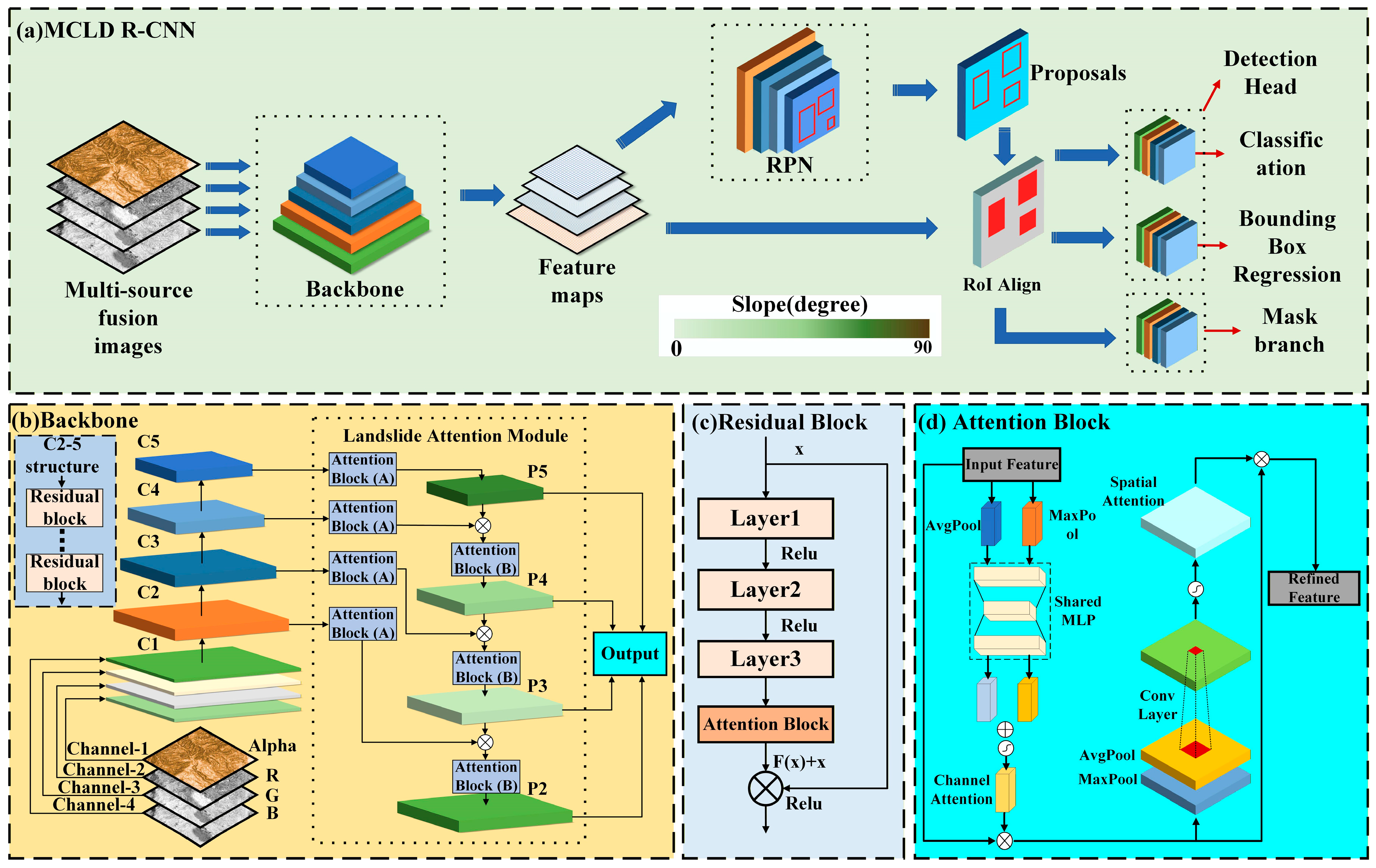
In this research, an instance segmentation model with multi-channel input, termed MCLD R-CNN (Multi-Channel Landslide Detection R-CNN), is constructed upon the Mask R-CNN architecture [49]. MCLD R-CNN functions as a two-stage framework for instance segmentation [50,51]. It is capable of performing both object detection and mask generation simultaneously, thereby enabling precise identification and contour extraction of active landslide areas. The model accommodates multi-channel data input to fully exploit the rich information contained in multi-source fusion imagery. Moreover, a Landslide Attention Module was embedded within the network architecture to strengthen the model’s capacity for extracting and identifying active landslide features. As illustrated in Figure 6a, the MCLD R-CNN primarily consists of a backbone network, a Region Proposal Network (RPN), an RoI Align layer, a detection head, and a mask branch. The following section focuses on the structural improvements incorporated into the proposed model.

3.3.1. Backbone Network of MCLD R-CNN

The backbone network mainly serves to capture image features at multiple scales from the given input samples. As shown in Figure 6b, it mainly comprises an improved Residual Network (ResNet) [52] and a Landslide Attention Module. The former supports multi-channel data input and is capable of extracting hierarchical features from the input. The latter aims to integrate multi-level features while maintaining both semantic information from higher layers and detailed characteristics from lower ones.

As the depth of convolutional neural networks increases, issues such as vanishing and exploding gradients may arise, impeding the efficiency of model training. ResNet addresses these issues by introducing residual learning and shortcut connections, enabling the stable training of deep networks while significantly enhancing feature extraction capabilities. The core component of the ResNet architecture is the residual block, and by stacking multiple residual blocks, ResNet networks of varying depths can be constructed. The residual block is defined mathematically as follows:

$$b=Y\left(a,\left\{K_i\right\}\right)+K_{s}a$$

(5)

In this equation, a denotes the input to the residual block, Y (a, {K_i}) represents the residual function, and K_S is a 1 × 1 convolution kernel employed to align the dimensions of the input a with the output.

In this work, the ResNet training architecture is adapted to handle multi-channel input data. Additionally, attention blocks (Figure 6c) are integrated into the residual blocks to improve the network’s ability to extract features associated with active landslides [53]. The fundamental structure of the attention block, shown in Figure 6d, comprises a channel attention component and a spatial attention component. The channel attention component assigns importance weights to each channel, thereby strengthening the feature responses of the most relevant channels. In contrast, the spatial attention component computes importance weights for each spatial position, enabling the model to concentrate on the target regions. The fundamental computational formulas for channel and spatial attention are given below:

$$C_{cha}(Y)=Sig(MLP(AP(Y))+MLP(MP(Y)))$$

(6)

$$Y_{cha}=C_{cha}(Y)\otimes Y$$

(7)

$$C_{spa}(Y_{cha})=Sig(Con{v}^{7\times 7}([AP(Y_{cha});MP(Y_{cha})]))$$

(8)

$$Y_{out}=C_{spa}(Y_{cha})\otimes Y_{cha}$$

(9)

In the formula, C_cha and C_spa denote the channel and spatial attention components, respectively. Y is the input feature map, Y_cha is the feature map after channel attention, and Y_out represents the final output. AP(Y) and MP(Y) perform average and max pooling over the spatial dimensions H × W. MLP denotes a shared two-layer fully connected network. Conv ^7×7 denotes a 7 × 7 convolution, and Sig is the Sigmoid function that normalizes weights to [0, 1].

The original ResNet architecture outputs only the highest-level features, which are highly abstract and often lack detailed information about target objects. This constraint limits the model’s capacity to precisely detect active landslides with diverse shapes and scales. To overcome this limitation, this study proposes a Landslide Attention Module that combines attention blocks with a Feature Pyramid Network (FPN) structure [54]. As illustrated in Figure 6b, the Landslide Attention Module initially extracts multi-level features via lateral connections and refines the original features using Attention Block A. Then, starting from the topmost feature level, a top-down pathway with upsampling is employed to progressively fuse the higher-level features with those from lower levels. Attention block B is applied to reinforce the fused features. This design facilitates the flow of high-level semantic information to lower layers while concurrently strengthening features relevant to the target. In contrast to relying solely on a single high-level feature map, integrating multi-level features retains both semantic and fine-grained information from the input. This integration enhances the model’s ability to detect and localize objects, thereby improving the accuracy of both detection and mask generation.

3.3.2. The Improved RPN and the RoI Align Layer

The RPN produces candidate regions of interest, represented as bounding boxes that potentially contain objects, using the feature maps generated by the backbone network. Its core task is to determine whether an anchor box contains an object. Additionally, it adjusts the anchor box’s position and size through a regression branch, bringing it closer to the true object bounding box. Finally, high-quality candidate regions are selected through Non-Maximum Suppression.

The specific process is as follows:

(1)

Multiple rectangular anchor boxes with varying scales and aspect ratios are predefined for each pixel in the input feature map. For the pixel located at (i, j) in the feature map, the center coordinates of its corresponding anchor boxes are defined as:

$$x_c=(i+0.5)\times s$$

(10)

$$y_c=(j+0.5)\times s$$

(11)

In the formula, s represents the total stride of the backbone network.

(2)

Through convolutional processing in the RPN head, the network outputs the objectness score for each anchor box and the bounding box offsets, which determine the candidate regions for subsequent processing. The RPN employs a joint loss function that includes both classification and regression components:

$$L{(\{p_i\},\{t_i\})}_{RPN}={\displaystyle \frac{1}{N_{cls}}}{\displaystyle \sum _i{L}_{cls}(p_i,p_i^{*})+\lambda \frac{1}{N_{reg}}{\displaystyle \sum _i{p}_i^{*}{L}_{reg}(t_i,t_i^{*})}}$$

(12)

In the formula, L_cls denotes the binary cross-entropy term, while L_reg corresponds to the smooth L1 regression loss. p_i indicates the predicted probability for the foreground class, and $p_i^{*}$∈ {0, 1} is the corresponding ground-truth label. t_i and $t_i^{*}$ represent the predicted and reference bounding-box offsets, respectively. N_cls and N_reg serve as normalization terms, and λ acts as a weighting coefficient to balance the two loss components.

The RoI Align layer addresses the key issue of feature alignment for candidate regions through precise coordinate mapping and feature sampling mechanisms. The primary role of this module is to precisely project the Region of Interest (RoI) coordinates from the original image domain onto the feature map domain. It then extracts the corresponding target regions from the feature maps generated by the backbone network. By leveraging bilinear interpolation, RoI Align preserves sub-pixel spatial information during feature sampling. This effectively avoids the feature misalignment problems caused by the double quantization in the traditional RoI Pool method [55]. As a result, it significantly improves spatial alignment accuracy and enhances both the smoothness of pixel-level mask boundaries and the precision of object localization.

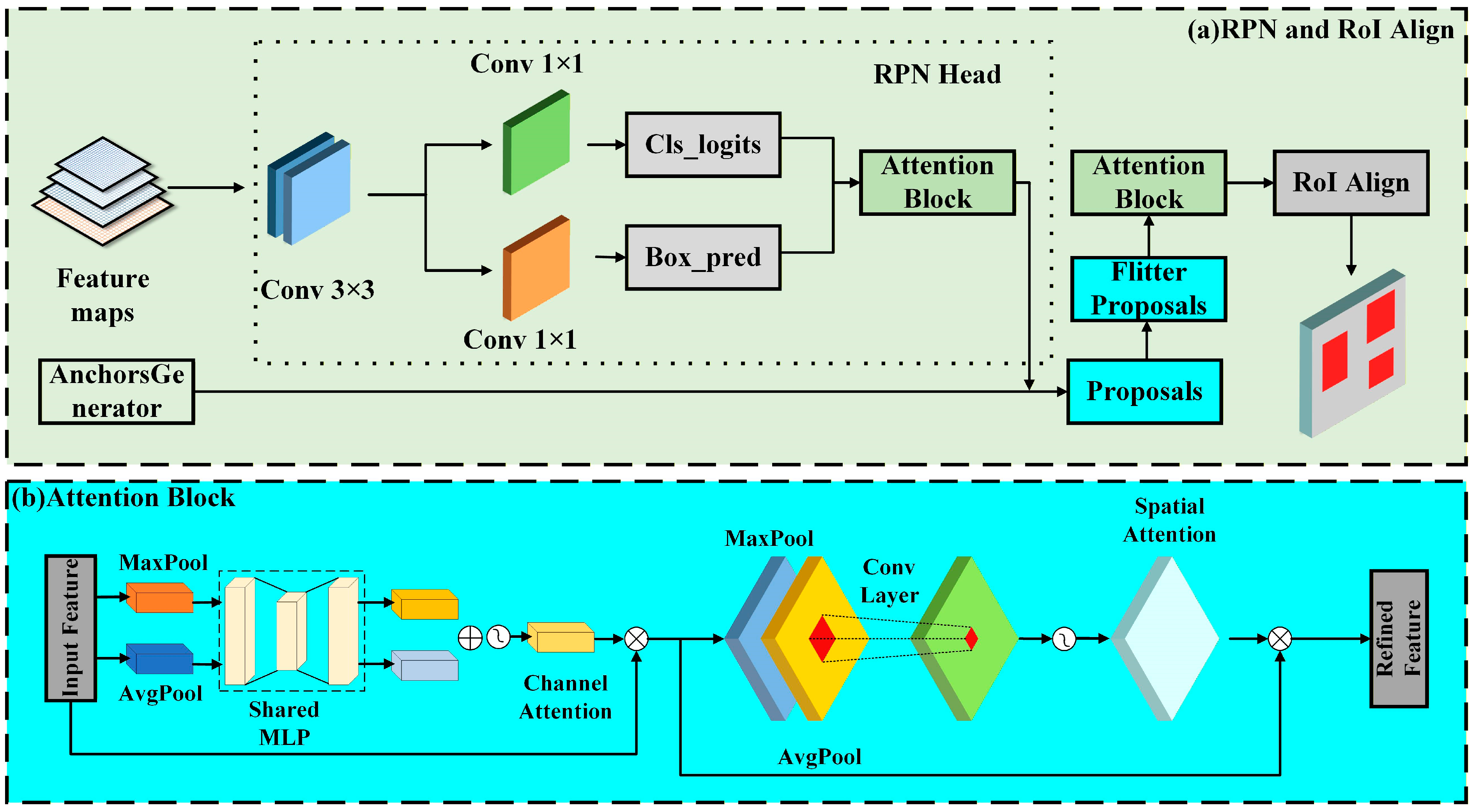
As shown in Figure 7, incorporating attention blocks into both the RPN and RoI Align layers optimizes proposal matching and region selection. This enhancement improves the quality of candidate bounding boxes from the RPN and strengthens feature alignment in the RoI Align layer. Consequently, it yields more precise feature representations, enhancing subsequent detection and segmentation performance.

3.4. Model Performance Evaluation Metrics

Five evaluation metrics were employed to assess model performance. The selected metrics include Precision (P), Recall (R), F1-score, mean Average Precision at IoU = 0.5 (mAP₅₀), and mean Average Precision computed over IoU thresholds from 0.5 to 0.95 (mAP_50–95). Among these metrics, P measures the ratio of correctly identified positive samples to the total number of samples predicted as positive by the model. R measures the proportion of actual positive samples that are correctly detected by the model. mAP₅₀ reflects object detection robustness and coarse localization, whereas mAP_50–95 evaluates the quality of high-precision bounding box regression and spatial fitting. The F1-score is employed to assess the harmonic balance between precision and recall, providing an integrated measure of the model’s overall performance. The computational formulations of these metrics are presented in Equations (10)–(13).

$$P=TP/(FP+TP)$$

(13)

$$R=TP/(FN+TP)$$

(14)

$$mAP={\displaystyle \frac{1}{c}}{\displaystyle \sum _{i=1}^c({\displaystyle {\int }_0^1{P}_i(R)dR})}$$

(15)

$$F1=2\times P\times R/(R+P)$$

(16)

In the above equations, TP denotes the number of true positive samples correctly identified as positive by the model, FP refers to false positive samples that are incorrectly classified as positive, and FN indicates false negative samples that are mistakenly predicted as negative. The variable c represents the total number of classes.

This study evaluates the performance of the MCLD R-CNN model from two perspectives: active landslide detection and segmentation. Detection performance assesses the model’s capability to accurately identify and localize active landslides, while segmentation performance assesses its capability to extract and refine object contours. Both aspects are evaluated using the five aforementioned performance metrics.

4. Results and Analysis of Experiments

4.1. Model Training Parameters

The experiments were conducted in a workstation environment using Python 3.12 as the programming language and PyTorch 1.13 as the deep learning framework. The workstation was equipped with an Intel i5-14600KF CPU and an NVIDIA GeForce RTX 4090D GPU, providing the computational resources necessary for model training and evaluation. The model was trained for 200 epochs with a batch size of 8 and a learning rate of 0.001. To comprehensively assess the performance of MCLD R-CNN, several instance segmentation models were included for comparative evaluation. To ensure the fairness and validity of the comparative experiments, a strict protocol covering both model architecture and training strategies was established. First, regarding architecture adaptation, the input layers of all baseline models were adapted to match the channel dimensions of the dataset. Specifically, for the multi-source fusion image dataset, the first convolutional layers were adjusted to accept four-channel inputs, ensuring that all models had equal access to the slope information. Second, regarding the training process, although hyperparameters such as epoch numbers and learning rates varied to accommodate the distinct convergence characteristics of one-stage (Yolo series) and two-stage (R-CNN series) architectures, the optimization objective remained consistent. Training was conducted for sufficient fixed epochs (as detailed in

Table 2. Training Configurations of Comparative Models.

Model	Epoch	Learning-Rate	Batch Size
Yolov8 [56]	1000	0.001	8
Yolov9 [57]	1000	0.001	8
Yolov11 [58]	1000	0.001	8
Yolov12 [59]	1000	0.001	8
Mask R-CNN-50 [49]	40	0.02	8
Mask R-CNN-101	40	0.02	8
Mask R-CNN-152	40	0.02	8

) to ensure full model convergence, which was assessed by monitoring the stabilization of validation loss and mAP curves. Crucially, the “best model” checkpoint for each method was selected based on the highest mAP₅₀ score achieved on the validation set during training, rather than relying on the final epoch weights. Furthermore, to eliminate data-related bias, an identical data augmentation pipeline was applied uniformly across all models. The models along with their respective training parameters are summarized in Table 2. For the Mask R-CNN variants, the designations ranging from 50 to 152 represent the varying depths of the backbone networks, corresponding to ResNet architectures with 50 to 152 layers.

4.2. Model Performance Comparison

4.2.1. Comparison of Performance Evaluation Metrics

Table 3. Quantitative Indicators for Each Model Under Different Data Sets.

Dataset	Model	Detection Performance					Segmentation Performance
		P	R	F1	mAP50	mAP50–95	P	R	F1	mAP50	mAP50–95
Defor mation rate image dataset	Yolov8	81.40	64.00	71.66	73.60	44.00	79.80	59.20	67.97	69.10	32.30
	Yolov9	94.60	87.00	90.64	93.30	72.80	93.50	82.60	87.71	90.20	57.50
	Yolov11	85.10	67.80	75.47	77.00	48.60	83.50	63.80	72.33	73.00	36.50
	Yo1ov12	85.50	67.40	75.38	77.40	50.10	85.10	65.60	74.09	75.10	38.70
	Maskrcnn-50	73.74	78.96	76.26	78.16	54.27	66.14	71.52	68.73	70.69	37.58
	Maskrcnn-101	75.46	79.67	77.51	79.24	55.31	67.46	72.53	69.90	72.20	38.39
	Maskrcnn-152	76.65	80.83	78.68	80.12	56.15	67.44	72.96	70.09	73.15	38.94
	Our model	93.95	95.93	94.93	95.00	61.86	87.06	89.98	88.50	91.25	45.18
Two- source fusion image dataset	Yolov8	84.60	66.10	74.21	76.80	46.70	85.50	64.40	73.46	75.10	39.10
	Yolov9	96.10	90.10	93.00	95.10	78.30	93.60	87.20	90.29	93.10	63.20
	Yolov11	83.10	72.10	77.21	80.50	52.70	85.40	68.10	75.78	78.50	43.30
	Yolov12	88.50	70.90	78.73	81.81	54.50	87.80	69.40	77.52	80.40	45.60
	Maskrcnn-50	81.04	84.71	82.83	84.29	59.31	76.73	80.63	78.63	80.33	45.79
	Maskrcnn-101	81.92	85.71	83.78	85.34	60.00	78.73	82.50	80.57	82.06	46.93
	Maskrcnn-152	82.90	86.39	84.60	84.99	60.60	78.24	82.22	80.18	81.19	46.65
	Our model	96.66	97.60	97.13	97.50	71.23	93.34	94.82	94.08	95.45	56.75
Multi-source fusion image dataset	Yolov8	92.80	82.30	87.24	90.60	64.00	92.80	77.30	84.34	87.70	51.80
	Yolov9	97.20	95.70	96.44	97.20	86.80	95.00	90.20	92.54	95.50	70.10
	Yolov11	89.90	79.30	84.27	87.60	60.20	89.20	76.70	82.48	85.70	49.80
	Yolov12	91.30	77.50	83.84	87.40	60.20	91.50	74.20	81.95	85.10	49.00
	Maskrcnn-50	83.08	85.67	84.35	86.10	60.10	78.63	81.54	80.06	82.10	47.20
	Maskrcnn-101	84.51	87.78	86.11	87.30	60.40	79.84	83.03	81.40	83.50	46.80
	Maskrcnn-152	83.01	86.00	84.48	86.00	60.20	78.01	81.45	79.69	82.50	47.20
	Our model	97.79	98.18	97.98	97.88	75.48	95.70	96.55	96.12	96.73	60.95

Underlined values represent the best metric for each dataset, while bold values denote the overall best performance across all datasets.

provides a summary of the detection and segmentation performance of each model across the three datasets. As shown in the tables:

(1)

For the same model across different datasets, the models trained with multi-source fusion images consistently show the best performance, while the models trained with deformation rate image datasets perform inferiorly. This indicates that training the model with fusion images yields better results, and as the variety of fused data increases, the model’s performance improves progressively. This is particularly evident in the mAP_50–95 metric, where the maximum improvements reached 45% (detection performance) and 60% (segmentation performance). Moreover, the Precision (detection performance) of our model improved from 93.95% on the deformation-only dataset to 97.79% on the multi-source dataset. This increase of nearly 4 percentage points signifies a substantial reduction in False Positives (FP), quantitatively confirming that fusing multi-source data effectively filters out confounding geological activities.

(2)

Across different models on the same dataset, MCLD R-CNN consistently demonstrates superior performance. Particularly in terms of R, F1, and mAP₅₀ metrics, it achieved the highest detection and segmentation scores across all datasets. In some datasets, it also achieved the highest P score, and the mAP_50–95 metric was only slightly lower than Yolov9. Therefore, based on these comparative results, it is evident that MCLD R-CNN offers the best overall performance.

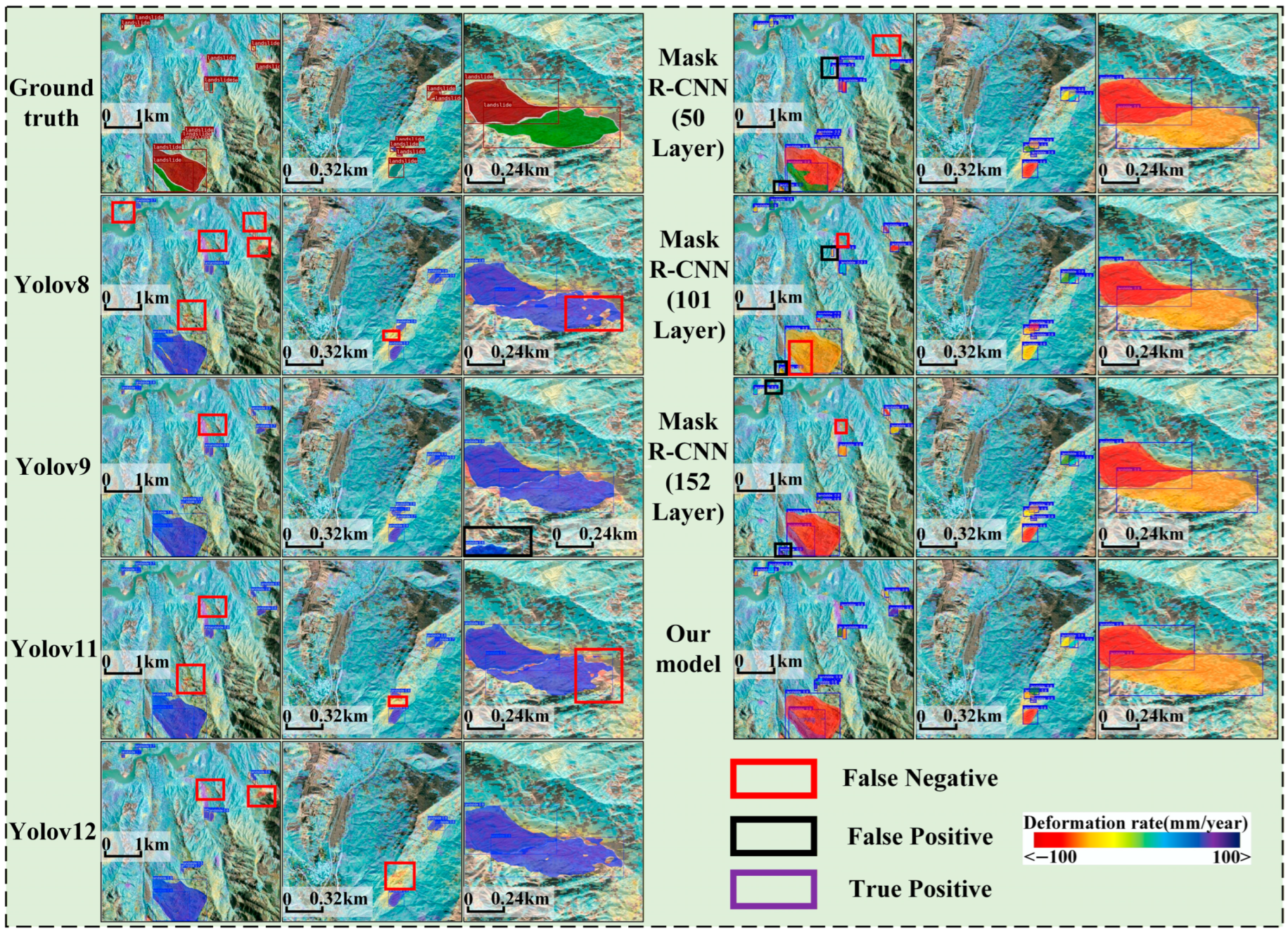
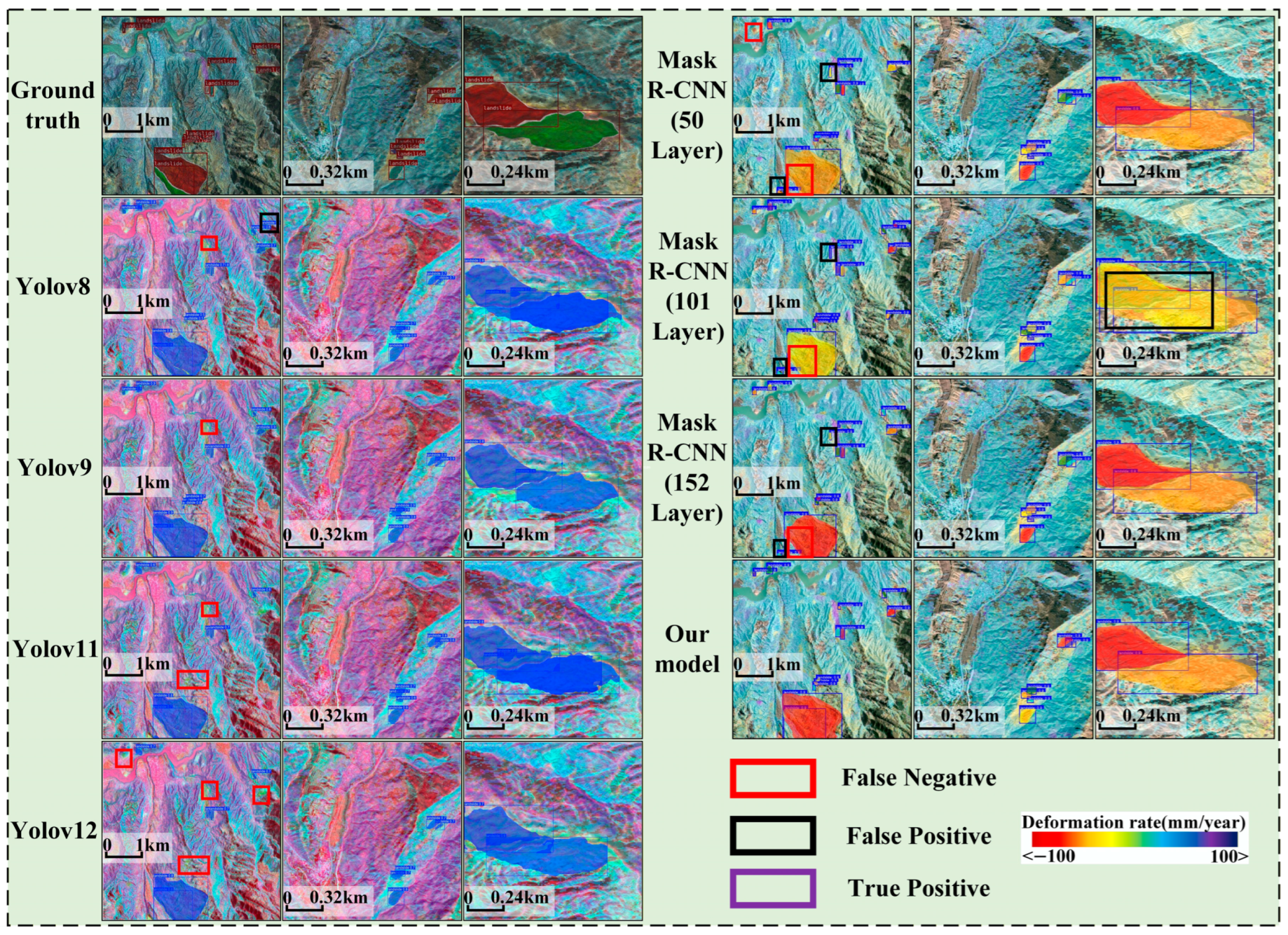
Figure 8, Figure 9 and Figure 10 illustrate the detection results of each model on images of varying scales across the different datasets. As observed in the figure:

(1)

In the deformation rate image dataset, all models showed varying levels of missed and false detections, which were particularly pronounced for small-scale images. This is primarily attributed to the relatively small spatial extent of most active landslides in these images, posing a challenge for the models to effectively extract features. The Yolov11 model exhibited the most severe detection errors, whereas MCLD R-CNN achieved an exceptionally low missed detection rate despite a few false positives. Segmentation performance across all models was generally poor, especially in large-scale images, where models struggled to outline complete landslide contours. This suggests that deformation rate features mainly assist in localization but are insufficient for determining precise coverage and contours.

(2)

In both the two-source and multi-source fusion image datasets, most models exhibited reduced missed and false detections, alongside significantly enhanced segmentation performance. Notably, models trained on multi-source fusion images demonstrated superior segmentation performance compared to those trained on two-source fusion image datasets. This indicates that multi-source imagery provides richer landslide-related features, thereby enhancing the model’s detection capability. However, it is notable that detection results for identical landslide instances were inconsistent across datasets. Specifically, models like Yolov8 and Yolov12 missed certain active landslides in the fusion images that they had correctly identified in other datasets. This phenomenon was primarily concentrated in small-scale images. A likely reason is that these models extract conflicting features from the fused images, rendering it difficult to distinguish whether a target is an active landslide. In summary, utilizing fusion imagery reduces detection errors, with the multi-source fusion image dataset yielding the most significant performance gains. The quantitative improvements shown in Table 3 effectively support this conclusion.

(3)

Across all datasets, our proposed model consistently maintained superior detection correctness and segmentation accuracy. This visual evidence directly demonstrates the performance advantages of our model, a finding further substantiated by the quantitative metrics analyzed above.

4.2.2. Model Training Curve Analysis

Figure 11 shows the mAP₅₀ and Loss curves for each model across different datasets. Since the training epochs vary across models, data from the first 100 epochs are selected for comparison. As observed in the figure:

(1)

Within the same model, models trained with fusion images generally exhibit better performance and faster convergence. As the variety of fused data increases, the training results progressively improve. This is particularly evident in the Yolo series models. Therefore, using multi-source fused images for training significantly enhances training efficiency, enabling the model to attain improved performance with fewer training epochs.

(2)

Comparing Figure 11 with Table 3, it is clear that both MCLD R-CNN and Yolov9 models exhibit superior detection performance, but the former converges faster. Although Mask R-CNN has the fastest convergence speed, its detection performance is relatively weaker. Therefore, the model proposed in this study achieves a balance between convergence speed and detection performance. By leveraging multi-source fusion images, the training time of detection models can be reduced, thereby enhancing the efficiency of landslide detection.

4.3. Ablation Experiment

The Landslide Attention Module serves as a crucial component of MCLD R-CNN, enhancing the model’s capability to extract and identify landslide-related features. To analyze its contribution to the landslide detection process, we trained and evaluated a model without this module.

Table 4. Quantitative results of the ablation experiment.

Index	Att	Layers	Par	FLOPs	P	R	mAP50	mAP50–95	F1
Det	No	50	43.98 M	129.46 G	96.48	97.60	97.26	68.94	97.03
	Yes	50	46.51 M	201.97 G	97.79	98.18	97.88	75.48	97.98
Seg	No	50	43.98 M	129.46 G	92.35	93.82	94.52	54.99	93.07
	Yes	50	46.51 M	201.97 G	95.70	96.55	96.73	60.95	96.12

Att denotes the attention module, Par denotes the parameter count, and FLOPs corresponds to the computational complexity.

presents the model’s performance in detecting landslides using the multi-source fusion image dataset. As indicated in the table, eliminating the Landslide Attention Module resulted in a noticeable reduction in the model’s detection and segmentation performance across all evaluation metrics, with the mAP_50–95 metric experiencing the largest decrease, dropping by 8.7% (detection performance) and 9.8% (segmentation performance). This finding suggests that the Landslide Attention Module is essential for enhancing the overall performance of the model. Figure 12 displays the attention heatmaps generated by the model along with the corresponding detection results. As shown in the figure:

(1)

The visualization demonstrates that the attention module operates as a dual-functional filter. While it intensifies the feature response in target regions (indicated by “hot” red colors), it simultaneously suppresses activation in non-landslide regions (indicated by “cool” blue colors). The Sigmoid activation function within the module acts as a gate, assigning near-zero weights to complex background features such as rivers, vegetation, and stable slopes. This effectively “mutes” the interference from these areas, preventing them from being misclassified as foreground.

(2)

After removing the Landslide Attention Module, the model’s attention becomes randomly dispersed across the entire image, making it difficult to focus on the target. As a result, the model struggles to detect the landslide accurately and is more easily affected by irrelevant regions.

(3)

In certain cases, the model also focuses its attention on incorrect regions. For example, in the seventh sample image shown, the model concentrates on the river instead of the active landslide.

In summary, the model incorporating the Landslide Attention Module exhibits fewer missed and false detections, along with superior segmentation performance. This suggests that the module enables the model to concentrate more precisely on landslide areas while improving its capacity to identify and delineate landslide contours. Although the integration of the Landslide Attention Module leads to a higher computational burden and an increased number of parameters, as shown in Table 4, this trade-off is justified by its significant enhancement of model performance.

4.4. Evaluation of the Model’s Generalization Capability

To assess the model’s generalization ability, we selected the Longyangxia Reservoir area as an independent test site. This region is geographically disjoint from the training tiles. Using the established operational definition, we constructed a generalization test dataset comprising 300 image samples containing a total of 58 labeled active landslides.

Compared to the training region, the Longyangxia test site exhibits significantly more rugged terrain, featuring deep alpine canyons and steep bedrock slopes along the reservoir banks. Regarding land cover and climate, while both regions share a semi-arid climate with sparse vegetation, the test site presents more complex background interference due to the presence of the large water body (reservoir). Finally, regarding data acquisition, Sentinel-1 imagery was collected using identical acquisition parameters (IW mode, VV + VH) as the training data to strictly evaluate model transferability without sensor-related bias.

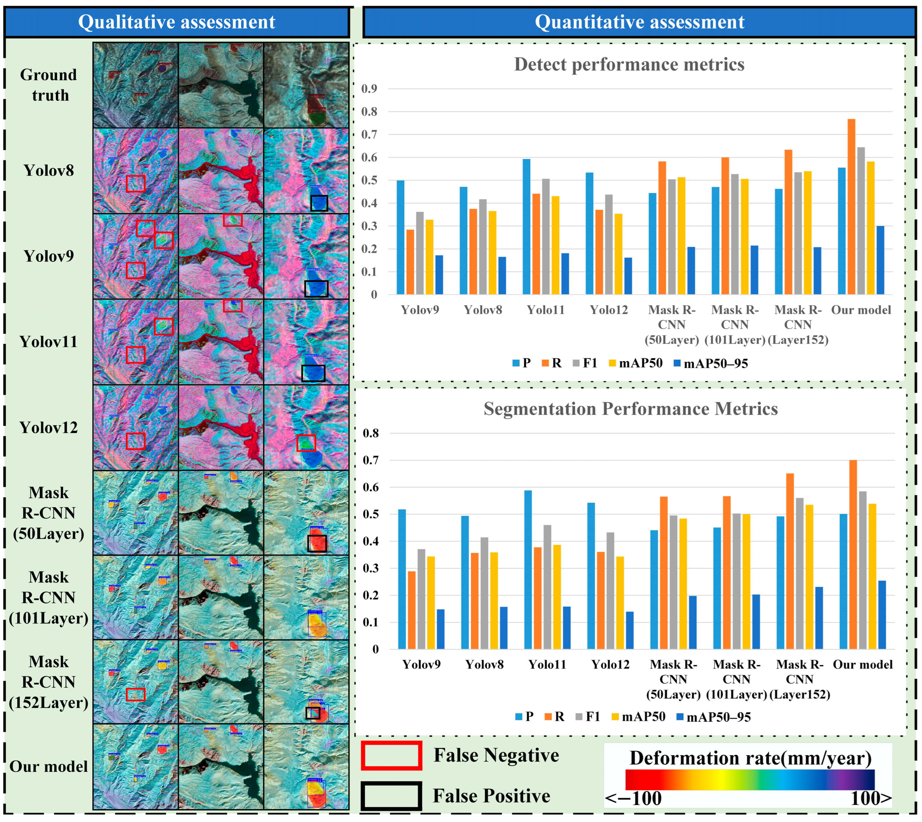
All models trained on the multi-source fusion image dataset were tested in this section, and the results are illustrated in Figure 13. As depicted in the figure:

(1)

MCLD R-CNN effectively detects most active landslides, demonstrating its high sensitivity to active landslides.

(2)

The Yolo series models exhibit a high number of missed detections, while Mask R-CNN exhibits poor segmentation performance. This indicates that these models struggle to adapt to unfamiliar images and can only achieve good performance on specific datasets.

(3)

The quantitative results presented on the right demonstrate that variations in landslide characteristics and data distribution relative to the training datasets led to decreased performance across all models. However, MCLD R-CNN still outperformed the others overall, with scores higher than the other models for all metrics except P.

In conclusion, compared to other models, MCLD R-CNN demonstrates better generalization capability. For detection tasks in specific regions, a small number of local samples can be used to fine-tune the model, enhancing its ability to detect active landslides in those particular areas.

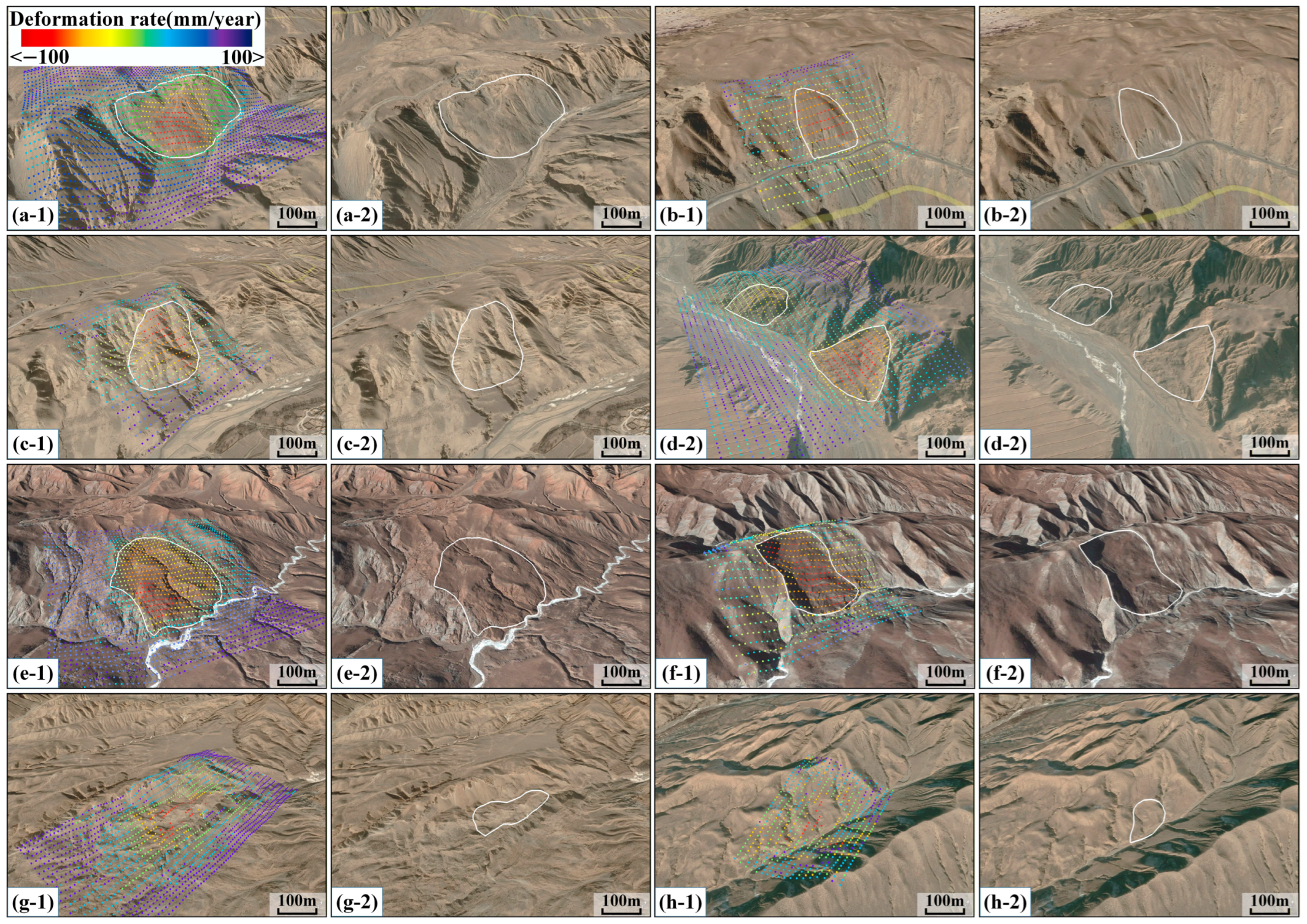
Figure 14 presents the InSAR deformation maps and optical imagery of typical cases identified within the test region. For the successfully detected active landslides, the boundaries delineated by the proposed model (white contour lines) align well with the actual terrain and topographic features, demonstrating the robustness and reliability of the model in identifying active landslides. However, the figure also illustrates typical failure cases (missed detections) to analyze the model’s limitations. As observed in the bottom row of Figure 14, these missed landslides are characterized by extremely sparse InSAR measurement points (coherent pixels) on the slope surface. The scarcity of deformation signals results in incomplete feature information, making it difficult for the model to distinguish the landslide from the background or to verify its activity status. This indicates that while the model generalizes well, its performance remains sensitive to the density and quality of the input InSAR observations.

5. Discussion

5.1. Advantages and Limitations of the Dataset and Method

Multi-source fusion image enables the efficient integration of heterogeneous information within a single tensor, with distinct remarkable advantages in active landslide detection tasks. Integrating multiple data modalities markedly strengthens the model’s capacity to identify landslide boundaries, deformation features, and fine-scale geomorphic variations. Moreover, such fused data substantially improves model convergence speed and training stability. This allows the network to achieve superior performance with fewer training epochs, which is especially valuable under limited computational resources.

Specifically, this study fuses multi-source data, including optical imagery, DEM-derived slope, and InSAR deformation. By integrating these along the channel dimension, we adopt a single-branch network for training. This design not only maintains computational efficiency but also systematically mitigates two persistent challenges in InSAR-based detection.

Firstly, it addresses the difficulty existing methods face in distinguishing active landslides from other ground deformations, thereby reducing false alarms. By enhancing data richness through fusion, the model can better locate active landslides. This improvement is quantitatively confirmed by the significant increase in the Precision (detection performance) of MCLD R-CNN. Specifically, precision rose from 93.95% on deformation-only data to 97.79% on multi-source fusion data, indicating a substantial reduction in false positives. Simultaneously, this approach improves boundary delineation, which is often limited by blurred edges in deformation maps. By incorporating optical texture and slope information, our method enhances feature representation and sharpens boundary definition. The increase in Segmentation mAP_50–95 of the proposed model (rising from 45.18% on deformation-only data to 60.95% on multi-source fusion data) serves as robust proof of this improvement.

Furthermore, to address the challenge of class imbalance, specific strategies were employed at the data level. Rigorous data augmentation techniques, including random vertical/horizontal flipping and rotation, were applied to the training dataset. This approach effectively increased the frequency and diversity of positive samples, directly contributing to the model’s notable balance between high Precision and Recall.

Nevertheless, this approach introduces greater complexity in data preprocessing, imposes higher demands on spatial co-registration accuracy, and may cause information loss during the fusion process, leading to partial feature attenuation. Future research will focus on reducing data loss, improving spatial alignment precision, and optimizing multimodal fusion strategies, with the goal of further enhancing model robustness and accuracy in complex geological environments.

5.2. Model Advantages and Limitations

Although MCLD R-CNN demonstrates superior detection and segmentation performance across three datasets as well as robust generalization capabilities, its performance on the high-precision localization metric mAP_50–95 is slightly lower than that of Yolov9. This discrepancy in localization accuracy is primarily attributed to two factors. First, differences in model architecture and regression loss play a role. Specifically, the Smooth L1 loss used by the two-stage MCLD R-CNN is less sensitive to fine-grained boundary adjustments for high-IoU samples than the dynamic label assignment and high-order IoU losses employed by Yolov9. Second, inherent limitations exist within the feature, as the bilinear interpolation in the RoI Align layer may cause slight feature smoothing at object edges. However, it is worth noting that compared to the standard Mask R-CNN baseline, the proposed modifications significantly mitigate this smoothing effect. As evidenced in Table 3, MCLD R-CNN achieves a Segmentation mAP_50–95 of 60.95%, a substantial improvement over the baseline’s 47.20%, indicating that the Landslide Attention Module effectively enhances edge feature representation before pooling.

Furthermore, through qualitative visual assessment (as seen in Figure 8, Figure 9, Figure 10 and Figure 13), we observed that while baseline models like Yolov9 tend to generate smoothed, convex masks to maximize IoU. In contrast, MCLD R-CNN produces boundaries with higher topographic conformity. It more accurately traces complex geological features. From a unified analytical perspective, MCLD R-CNN achieves a significantly higher Recall score than Yolov9, despite a slightly lower mAP_50–95. This reveals a distinct trade-off between extreme localization precision and comprehensive target capture. For active landslide detection, high recall holds greater practical value, as timely identifying potential hazards—even with slight positional deviations—is far more critical than missing high-risk targets. Future work will focus on addressing these limitations to further improve boundary optimization strategies.

6. Conclusions

This study constructed a multi-source fusion image dataset integrating optical remote sensing imagery, DEM-derived slope data, and InSAR deformation information for active landslide detection. Based on this dataset, a multi-channel instance segmentation model, termed MCLD R-CNN, was developed. The model was systematically evaluated and compared across three independent datasets. Experimental results demonstrate that training with the multi-source fusion image dataset significantly enhances both the detection performance and training convergence efficiency. These findings confirm the dataset’s effectiveness and superiority in active landslide detection. Across all evaluation metrics, MCLD R-CNN achieved the best overall performance. The incorporation of the Landslide Attention Module substantially enhanced the extraction and recognition of landslide-related features, resulting in higher sensitivity and responsiveness to active landslide regions. Moreover, MCLD R-CNN exhibited strong cross-dataset generalization capability, effectively adapting to diverse data sources and geological environments. Overall, the proposed approach provides a promising framework for large-scale, high-precision, and automated detection of active landslides, offering important scientific and practical value for the monitoring of landslide hazards and early warning.

Future work will aim to enhance the diversity of the fused datasets and optimize the efficiency of data fusion. In particular, we plan to introduce a dynamic data fusion mechanism and expand the input dimensionality of the multi-channel model to integrate additional sensing modalities. These efforts are intended to improve the model’s capacity for feature representation and its detection accuracy in complex and heterogeneous landslide environments.

References

1. Keefer, D.K.; Larsen, M.C. Assessing landslide hazards. Science 2007, 316, 1136–1138. [Google Scholar] [CrossRef]
2. Froude, M.J.; Petley, D.N. Global fatal landslide occurrence from 2004 to 2016. Nat. Hazards Earth Syst. Sci. 2018, 18, 2161–2181. [Google Scholar] [CrossRef]
3. Lan, H.; Liu, X.; Li, L.; Li, Q.; Tian, N.; Peng, J. Remote Sensing Precursors Analysis for Giant Landslides. Remote Sens. 2022, 14, 4399. [Google Scholar] [CrossRef]
4. Xu, Q.; Zhao, B.; Dai, K.; Dong, X.; Li, W.; Zhu, X.; Yang, Y.; Xiao, X.; Wang, X.; Huang, J.; et al. Remote sensing for landslide investigations: A progress report from China. Eng. Geol. 2023, 321, 107156. [Google Scholar] [CrossRef]
5. Santangelo, M.; Cardinali, M.; Rossi, M.; Mondini, A.C.; Guzzetti, F. Remote landslide mapping using a laser rangefinder binocular and GPS. Nat. Hazards Earth Syst. Sci. 2010, 10, 2539–2546. [Google Scholar] [CrossRef]
6. Guzzetti, F.; Mondini, A.C.; Cardinali, M.; Fiorucci, F.; Santangelo, M.; Chang, K.-T. Landslide inventory maps: New tools for an old problem. Earth Sci. Rev. 2012, 112, 42–66. [Google Scholar] [CrossRef]
7. Haneberg, W.C.; Cole, W.F.; Kasali, G. High-resolution lidar-based landslide hazard mapping and modeling, UCSF Parnassus Campus, San Francisco, USA. Bull. Eng. Geol. Environ. 2009, 68, 263–276. [Google Scholar] [CrossRef]
8. Kurtz, C.; Stumpf, A.; Malet, J.-P.; Gancarski, P.; Puissant, A.; Passat, N. Hierarchical extraction of landslides from multiresolution remotely sensed optical images. ISPRS J. Photogramm. Remote Sens. 2014, 87, 122–136. [Google Scholar] [CrossRef]
9. Pesci, A.; Teza, G.; Casula, G.; Loddo, F.; De Martino, P.; Dolce, M.; Obrizzo, F.; Pingue, F. Multitemporal laser scanner-based observation of the Mt. Vesuvius crater: Characterization of overall geometry and recognition of landslide events. ISPRS J. Photogramm. Remote Sens. 2011, 66, 327–336. [Google Scholar] [CrossRef]
10. Ferretti, A.; Prati, C.; Rocca, F. Permanent scatterers in SAR interferometry. IEEE Trans. Geosci. Remote Sens. 2001, 39, 8–20. [Google Scholar] [CrossRef]
11. Massonnet, D.; Rossi, M.; Carmona, C.; Adragna, F.; Peltzer, G.; Feigl, K.; Rabaute, T. The displacement field of the Landers earthquake mapped by radar interferometry. Nature 1993, 364, 138–142. [Google Scholar] [CrossRef]
12. Zebker, H.A.; Villasenor, J. Decorrelation in interferometric radar echoes. IEEE Trans. Geosci. Remote Sens. 1992, 30, 950–959. [Google Scholar] [CrossRef]
13. Zhuang, H.; Tang, Z.; Du, S.; Wang, P.; Fan, H.; Hao, M.; Tan, Z. Shadow-robust unsupervised flood mapping via GMM-enhanced generalized dual-polarization flood index and topography features. Int. J. Appl. Earth Obs. Geoinf. 2025, 143, 104787. [Google Scholar] [CrossRef]
14. Zhuang, H.; Wang, P.; Hao, M.; Fan, H.; Tan, Z. Flood inundation mapping in SAR images based on nonlocal polarization combination features. J. Hydrol. 2025, 646, 132326. [Google Scholar] [CrossRef]
15. Pedretti, L.; Bordoni, M.; Vivaldi, V.; Figini, S.; Parnigoni, M.; Grossi, A.; Lanteri, L.; Tararbra, M.; Negro, N.; Meisina, C. InterpolatiON of InSAR Time series for the dEtection of ground deforMatiOn eVEnts (ONtheMOVE): Application to slow-moving landslides. Landslides 2023, 20, 1797–1813. [Google Scholar] [CrossRef]
16. Rosen, P.A.; Hensley, S.; Joughin, I.R.; Li, F.K.; Madsen, S.N.; Rodriguez, E.; Goldstein, R.M. Synthetic aperture radar interferometry. Proc. IEEE 2000, 88, 333–382. [Google Scholar] [CrossRef]
17. Zhou, C.; Cao, Y.; Gan, L.; Wang, Y.; Motagh, M.; Roessner, S.; Hu, X.; Yin, K. A novel framework for landslide displacement prediction using MT-InSAR and machine learning techniques. Eng. Geol. 2024, 334, 107497. [Google Scholar] [CrossRef]
18. Dille, A.; Kervyn, F.; Handwerger, A.L.; d’Oreye, N.; Derauw, D.; Bibentyo, T.M.; Samsonov, S.; Malet, J.-P.; Kervyn, M.; Dewitte, O. When image correlation is needed: Unravelling the complex dynamics of a slow-moving landslide in the tropics with dense radar and optical time series. Remote Sens. Environ. 2021, 258, 112402. [Google Scholar] [CrossRef]
19. Kang, Y.; Lu, Z.; Zhao, C.; Qu, W. Inferring slip-surface geometry and volume of creeping landslides based on InSAR: A case study in Jinsha River basin. Remote Sens. Environ. 2023, 294, 113620. [Google Scholar] [CrossRef]
20. Lauknes, T.R.; Piyush Shanker, A.; Dehls, J.F.; Zebker, H.A.; Henderson, I.H.C.; Larsen, Y. Detailed rockslide mapping in northern Norway with small baseline and persistent scatterer interferometric SAR time series methods. Remote Sens. Environ. 2010, 114, 2097–2109. [Google Scholar] [CrossRef]
21. Wang, W.; Motagh, M.; Mirzaee, S.; Li, T.; Zhou, C.; Tang, H.; Roessner, S. The 21 July 2020 Shaziba landslide in China: Results from multi-source satellite remote sensing. Remote Sens. Environ. 2023, 295, 113669. [Google Scholar] [CrossRef]
22. LeCun, Y.; Bengio, Y.; Hinton, G. Deep learning. Nature 2015, 521, 436–444. [Google Scholar] [CrossRef]
23. Ma, Z.; Mei, G. Deep learning for geological hazards analysis: Data, models, applications, and opportunities. Earth Sci. Rev. 2021, 223, 103858. [Google Scholar] [CrossRef]
24. Wei, R.; Li, Y.; Li, Y.; Zhang, B.; Wang, J.; Wu, C.; Yao, S.; Ye, C. A universal adapter in segmentation models for transferable landslide mapping. ISPRS J. Photogramm. Remote Sens. 2024, 218, 446–465. [Google Scholar] [CrossRef]
25. Lu, W.; Hu, Y.; Zhang, Z.; Cao, W. A dual-encoder U-Net for landslide detection using Sentinel-2 and DEM data. Landslides 2023, 20, 1975–1987. [Google Scholar] [CrossRef]
26. Lu, Z.; Peng, Y.; Li, W.; Yu, J.; Ge, D.; Han, L.; Xiang, W. An Iterative Classification and Semantic Segmentation Network for Old Landslide Detection Using High-Resolution Remote Sensing Images. IEEE Trans. Geosci. Remote Sens. 2023, 61, 4408813. [Google Scholar] [CrossRef]
27. Gu, W.; Bai, S.; Kong, L. A review on 2D instance segmentation based on deep neural networks. Image Vis. Comput. 2022, 120, 104401. [Google Scholar] [CrossRef]
28. Lv, P.; Ma, L.; Li, Q.; Du, F. ShapeFormer: A Shape-Enhanced Vision Transformer Model for Optical Remote Sensing Image Landslide Detection. IEEE J. Sel. Top. Appl. Earth Obs. Remote Sens. 2023, 16, 2681–2689. [Google Scholar] [CrossRef]
29. Ullo, S.L.; Mohan, A.; Sebastianelli, A.; Ahamed, S.E.; Kumar, B.; Dwivedi, R.; Sinha, G.R. A New Mask R-CNN-Based Method for Improved Landslide Detection. IEEE J. Sel. Top. Appl. Earth Obs. Remote Sens. 2021, 14, 3799–3810. [Google Scholar] [CrossRef]
30. Cai, J.; Zhang, L.; Dong, J.; Guo, J.; Wang, Y.; Liao, M. Automatic identification of active landslides over wide areas from time-series InSAR measurements using Faster RCNN. Int. J. Appl. Earth Obs. Geoinf. 2023, 124, 103516. [Google Scholar] [CrossRef]
31. Guo, H.; Yi, B.; Yao, Q.; Gao, P.; Li, H.; Sun, J.; Zhong, C. Identification of Landslides in Mountainous Area with the Combination of SBAS-InSAR and Yolo Model. Sensors 2022, 22, 6235. [Google Scholar] [CrossRef] [PubMed]
32. Zhang, T.; Zhang, W.; Cao, D.; Yi, Y.; Wu, X. A New Deep Learning Neural Network Model for the Identification of InSAR Anomalous Deformation Areas. Remote Sens. 2022, 14, 2690. [Google Scholar] [CrossRef]
33. Chen, L.-C.; Zhu, Y.; Papandreou, G.; Schroff, F.; Adam, H. Encoder-Decoder with Atrous Separable Convolution for Semantic Image Segmentation. In Proceedings of the European Conference on Computer Vision, Munich, Germany, 8–14 September 2018; pp. 833–851. [Google Scholar]
34. Chen, X.; Yao, X.; Zhou, Z.; Liu, Y.; Yao, C.; Ren, K. DRs-UNet: A Deep Semantic Segmentation Network for the Recognition of Active Landslides from InSAR Imagery in the Three Rivers Region of the Qinghai–Tibet Plateau. Remote Sens. 2022, 14, 1848. [Google Scholar] [CrossRef]
35. Chen, X.; Zhao, C.; Liu, X.; Zhang, S.; Xi, J.; Khan, B.A. An Embedding Swin Transformer Model for Automatic Slow-Moving Landslide Detection Based on InSAR Products. IEEE Trans. Geosci. Remote Sens. 2024, 62, 5223915. [Google Scholar] [CrossRef]
36. Chen, H.; He, Y.; Zhang, L.; Yang, W.; Liu, Y.; Gao, B.; Zhang, Q.; Lu, J. A Multi-Input Channel U-Net Landslide Detection Method Fusing SAR Multisource Remote Sensing Data. IEEE J. Sel. Top. Appl. Earth Obs. Remote Sens. 2023, 17, 1215–1232. [Google Scholar] [CrossRef]
37. Li, X.; Guo, X.; Li, W. Mechanism of Giant Landslides from Longyangxia Valley to Liujiaxia Valley along Upper Yellow River. J. Eng. Geol. 2011, 19, 516–529. [Google Scholar] [CrossRef]
38. Du, J.; Li, Z.; Song, C.; Zhu, W.; Ji, Y.; Zhang, C.; Chen, B.; Su, S. InSAR-Based Active Landslide Detection and Characterization Along the Upper Reaches of the Yellow River. IEEE J. Sel. Top. Appl. Earth Obs. Remote Sens. 2023, 16, 3819–3830. [Google Scholar] [CrossRef]
39. Peng, J.; Lan, H.; Qian, H.; Wang, W.; Li, R.; Li, Z.; Zhuang, J.; Liu, X.; Liu, S. Scientific Research Framework of Livable Yellow River. J. Eng. Geol. 2020, 28, 189–201. [Google Scholar] [CrossRef]
40. Yin, Z.; Cheng, G.; Hu, G.; Wei, G.; Wang, Y. Preliminary Study on Characteristic and Mechanism of Super-Large Landslides in Upper Yellow River Since Late-Pleistocene. J. Eng. Geol. 2010, 18, 41. [Google Scholar] [CrossRef]
41. Yin, Z.; Qin, X.; Zhao, W. Characteristics of Landslides from Sigou Gorge to Lagan Gorge in the Upper Reaches of Yellow River. In Proceedings of the Third World Landslide Forum, Beijing, China, 2–6 June 2014; pp. 397–406. [Google Scholar]
42. Berardino, P.; Fornaro, G.; Lanari, R.; Sansosti, E. A new algorithm for surface deformation monitoring based on small baseline differential SAR interferograms. IEEE Trans. Geosci. Remote Sens. 2002, 40, 2375–2383. [Google Scholar] [CrossRef]
43. Wegmller, U.; Strozzi, T.; Wiesmann, A. GAMMA SAR and interferometric processing software. In Proceedings of the ERS-Envisat Symposium, Gothenburg, Sweden, 16–20 October 2000. [Google Scholar]
44. Xue, F.; Lv, X.; Dou, F.; Yun, Y. A Review of Time-Series Interferometric SAR Techniques: A Tutorial for Surface Deformation Analysis. IEEE Geosci. Remote Sens. Mag. 2020, 8, 22–42. [Google Scholar] [CrossRef]
45. Hooper, A. A multi-temporal InSAR method incorporating both persistent scatterer and small baseline approaches. Geophys. Res. Lett. 2008, 35, L16302. [Google Scholar] [CrossRef]
46. Li, Y.; Zhang, Y.; Su, X.; Zhao, F.; Liang, Y.; Meng, X.; Jia, J. Early identification and characteristics of potential landslides in the Bailong River Basin using InSAR technique. Natl. Remote Sens. Bull. 2021, 25, 677–690. [Google Scholar] [CrossRef]
47. He, Y.; Wang, W.; Zhang, L.; Chen, Y.; Chen, Y.; Chen, B.; He, X.; Zhao, Z. An identification method of potential landslide zones using InSAR data and landslide susceptibility. Geomat. Nat. Hazards Risk 2023, 14, 2185120. [Google Scholar] [CrossRef]
48. Lin, T.-Y.; Maire, M.; Belongie, S.; Hays, J.; Perona, P.; Ramanan, D.; Dollár, P.; Zitnick, C.L. Microsoft COCO: Common Objects in Context. In Proceedings of the European Conference on Computer Vision, Zurich, Switzerland, 6–12 September 2014; pp. 740–755. [Google Scholar]
49. He, K.; Gkioxari, G.; Dollár, P.; Girshick, R. Mask R-CNN. In Proceedings of the 2017 IEEE International Conference on Computer Vision (ICCV), Venice, Italy, 22–29 October 2017; pp. 2980–2988. [Google Scholar]
50. Brabandere, B.D.; Neven, D.; Gool, L.V. Semantic Instance Segmentation with a Discriminative Loss Function. arXiv 2017. [Google Scholar] [CrossRef]
51. Hariharan, B.; Arbeláez, P.; Girshick, R.; Malik, J. Simultaneous Detection and Segmentation. In Proceedings of the European Conference on Computer Vision, Zurich, Switzerland, 6–12 September 2014; pp. 297–312. [Google Scholar]
52. He, K.; Zhang, X.; Ren, S.; Sun, J. Deep Residual Learning for Image Recognition. In Proceedings of the 2016 IEEE Conference on Computer Vision and Pattern Recognition (CVPR), Las Vegas, NV, USA, 27–30 June 2016; pp. 770–778. [Google Scholar]
53. Woo, S.; Park, J.; Lee, J.-Y.; Kweon, I.S. CBAM: Convolutional Block Attention Module. In Proceedings of the 15th European Conference on Computer Vision (ECCV), Munich, Germany, 8–14 September 2018; pp. 3–19. [Google Scholar]
54. Lin, T.-Y.; Dollár, P.; Girshick, R.; He, K.; Hariharan, B.; Belongie, S. Feature Pyramid Networks for Object Detection. In Proceedings of the 2017 IEEE Conference on Computer Vision and Pattern Recognition (CVPR), Honolulu, HI, USA, 21–26 July 2017; pp. 936–944. [Google Scholar]
55. Ren, S.; He, K.; Girshick, R.; Sun, J. Faster R-CNN: Towards Real-Time Object Detection with Region Proposal Networks. IEEE Trans. Pattern Anal. Mach. Intell. 2017, 39, 1137–1149. [Google Scholar] [CrossRef]
56. Varghese, R.; M., S. YOLOv8: A Novel Object Detection Algorithm with Enhanced Performance and Robustness. In Proceedings of the 2024 International Conference on Advances in Data Engineering and Intelligent Computing Systems (ADICS), Chennai, India, 18–19 April 2024; pp. 1–6. [Google Scholar]
57. Wang, C.-Y.; Yeh, I.-H.; Mark Liao, H.-Y. YOLOv9: Learning What You Want to Learn Using Programmable Gradient Information. In Proceedings of the European Conference on Computer Vision, Milan, Italy, 29 September–4 October 2024; pp. 1–21. [Google Scholar]
58. Khanam, R.; Hussain, M. YOLOv11: An Overview of the Key Architectural Enhancements. arXiv 2024. [Google Scholar] [CrossRef]
59. Tian, Y.; Ye, Q.; Doermann, D. YOLOv12: Attention-Centric Real-Time Object Detectors. arXiv 2025. [Google Scholar] [CrossRef]
Figure 1. Experimental Workflow.
Remotesensing 18 00126 g001
Figure 2. Research region. The red and blue rectangles represent the ascending and descending track image coverage areas, respectively.
Remotesensing 18 00126 g002
Figure 3. Multi-source fusion image processing flow. The black arrows represent the fusion process, the blue arrows indicate landslide target localization and mask drawing, and the red arrows represent the dataset label creation.
Remotesensing 18 00126 g003
Figure 4. Spatial distribution of active landslides within the study region. Red and blue boxes denote landslides detected from ascending and descending track imagery, respectively.
Remotesensing 18 00126 g004
Figure 5. Examples from each dataset.
Remotesensing 18 00126 g005
Figure 6. MCLD R-CNN. (a) illustrates the overall architecture of the MCLD R-CNN model. (b) illustrates the backbone network structure used for extracting target features. (c) depicts the structure of the improved residual block that makes up the backbone network. (d) demonstrates the attention block used to build the backbone network.
Remotesensing 18 00126 g006
Figure 7. Improved RoI Align Layer and RPN. (a) illustrates the framework composition of the RoI Align layers and RPN. (b) depicts the attention block incorporated into the framework.
Remotesensing 18 00126 g007
Figure 8. Detection results on the deformation rate image dataset.
Remotesensing 18 00126 g008
Figure 9. Detection results on the two-source fusion image dataset.
Remotesensing 18 00126 g009
Figure 10. Detection results on the multi-source fusion image dataset. To improve visual clarity, MCLD R-CNN uses images with a transparency channel for landslide detection, but presents the prediction results on RGB-format images.
Remotesensing 18 00126 g010
Figure 11. Training curves of each model for the first 100 epochs across three datasets.
Remotesensing 18 00126 g011
Figure 12. Heatmaps and detection results before and after introducing the landslide attention mechanism.
Remotesensing 18 00126 g012
Figure 13. Model Generalization Capability Test Results.
Remotesensing 18 00126 g013
Figure 14. InSAR results (subgraphs with suffix-1) and Google Earth optical images (subgraphs with suffix-2) of representative landslide cases in the test area. (af) illustrate successfully detected active landslides, where white lines indicate the delineated boundaries. (g,h) represent failure cases (missed detections).
Remotesensing 18 00126 g014