On the Potential of Bayesian Neural Networks for Estimating Chlorophyll-a Concentration from Satellite Data

Abstract

This work introduces the use of Bayesian Neural Networks (BNNs) for inferring chlorophyll-a concentration ([CHL-a]) from remotely sensed data. BNNs are probabilistic models that associate a probability distribution to the neural network parameters and rely on Bayes’ rule for training. The performance of the proposed probabilistic model is compared to that of standard ocean color algorithms, namely ocean color 4 (OC4) and ocean color index (OCI). An extensive in situ bio-optical dataset was used to train and validate the ocean color models. In contrast to established methods, the BNN allows for enhanced modeling flexibility, where different variables that affect phytoplankton phenology or describe the state of the ocean can be used as additional input for enhanced performance. Our results suggest that BNNs perform at least as well as established methods, and they could achieve 20–40% lower mean squared errors when additional input variables are included, such as the sea surface temperature and its climatological mean alongside the coordinates of the prediction. The BNNs offer means for uncertainty quantification by estimating the probability distribution of [CHL-a], building confidence in the [CHL-a] predictions through the variance of the predictions. Furthermore, the output probability distribution can be used for risk assessment and decision making through analyzing the quantiles and shape of the predicted distribution.

1. Introduction

Phytoplankton are a diverse group of microscopic photosynthetic organisms that play a crucial role in marine ecosystems, serving as the foundation of the marine food web [1]. Their pivotal role extends to the cycling of carbon, oxygen, nitrogen, and other elements between the atmosphere and the ocean [2,3]. Phytoplankton also act as climate regulators by absorbing substantial amounts of atmospheric carbon dioxide during photosynthesis, thereby mitigating the impacts of greenhouse gas emissions on the planet’s climate system [4,5,6]. Apart from their ecological and biogeochemical importance, changes in phytoplankton phenology can have direct impacts on human societies by influencing the survival of fish larvae and consequently fish stocks [7]. Harmful algal blooms (HABs), for instance, can release toxins that accumulate in seafood, posing threats to human health and causing disruptions in local economies [8,9]. It is, therefore, important to understand phytoplankton dynamics and identify changes to their seasonality and abundance.

Monitoring phytoplankton through remote sensing is important to study their distribution, abundance, and productivity across the world oceans and inland waters [10]. Remote sensing enables the acquisition of high-resolution data on large spatial and temporal scales, providing a comprehensive understanding of the processes governing phytoplankton dynamics [11]. A key advantage of remote sensing lies in its capacity to offer synoptic coverage of the ocean surface, surpassing the limitations of traditional sampling methods [12]. This facilitates detecting spatial and temporal patterns in phytoplankton abundance and productivity, as well as the identification of ecological hotspots [13] and their responses to global environmental changes, such as oceanic warming, ocean acidification, and eutrophication [14]. Remotely sensed data can also be utilized to calibrate and validate ocean biogeochemical models, which are crucial for predicting the responses of marine ecosystems to global environmental changes [15].

Ocean color algorithms are analytical tools that harness satellite imagery to estimate the concentrations of phytoplankton, sediment, and dissolved organic matter in the oceans. These algorithms operate on the principle of light absorption and scattering by various components present in the water, which influence the observed color of light reflected from the ocean’s surface [16]. To estimate phytoplankton concentration, these algorithms leverage the unique spectral characteristics exhibited by its pigment. Chlorophyll-a, the dominant photosynthetic pigment found in most phytoplankton, displays a distinctive optical signature, with high absorption of blue and red light and relatively high reflection of green light [17,18]. By utilizing the ratio (or difference) in blue to green light reflected by the ocean’s surface, these algorithms can derive estimates of chlorophyll-a concentration ([CHL-a]), thereby inferring the abundance of phytoplankton [16]. Recent advances in satellite technology and algorithm development have significantly improved the accuracy of these empirical algorithms [19,20]. However, the performance of ocean color models can still vary depending on the studied environmental conditions, with some regions posing greater challenges [19]. Furthermore, standard ocean color models rely on curve fitting noisy data using a polynomial function typically applied on limited datasets, providing no uncertainty estimates associated with the predictions. Studies evaluating the performance of ocean color algorithms generally indicate reasonable estimates across a range of conditions, though their accuracy can be affected by factors such as cloud cover, atmospheric interference, bottom reflectance, and the presence of other water constituents; for example, in rivers and estuaries [21,22].

Neural networks have emerged as a promising approach for analyzing complex remote sensing data due to their ability to recognize patterns within the data. A notable example is the Case2R algorithm, which leverages inverse modeling techniques to estimate [CHL-a] and total suspended matter from normalized water-leaving reflectance using an Inverse Radiative Transfer Model–Neural Network (IRTM-NN) [23]. Convolutional neural networks and artificial neural networks have also shown promising results in accurately estimating [CHL-a], with some studies reporting improved accuracy compared to traditional ocean color algorithms [24,25,26,27]. These methods provide deterministic estimates of [CHL-a] despite the inherent noise in the dataset, which arises from various sources of error in collecting [CHL-a] samples and imperfections in remotely sensed imagery, among others. On the other hand, a branch of deep learning explores probabilistic neural network models, which allow for uncertainty quantification and stochastic model evaluation [28].

Bayesian Neural Networks (BNNs) are a class of neural networks that incorporate probabilistic modeling to capture uncertainty in their predictions using Bayes’ rule [29]. In a BNN, the network’s parameters are treated as random variables by associating a probability distribution with the model parameters. Training these networks involves incorporating prior distributions over the weights, which are then updated using Bayesian inference techniques such as Markov Chain Monte Carlo (MCMC) or variational methods [30]. By accounting for uncertainty, BNNs enable more efficient and robust predictions, particularly in scenarios with limited data or complex datasets [31]. They present significant value particularly to ocean color models due to the uncertainty involved in the data acquisition and processing, where remotely sensed data are noisy, in situ measurements are not exact, and satellite image processing is extensively parameterized, to name a few of the challenges.

Bayesian models, including BNNs, offer significant advantages over deterministic models, such as integrating prior knowledge, estimating uncertainties through probability distributions [32]. Furthermore, the Bayesian framework is inherently robust to overfitting, as it models the underlying probabilistic distribution of the data rather than fitting the data. BNNs have found applications across various fields, including computer vision [33], natural language processing [34], robotics [35], and healthcare [36], where reliable uncertainty estimates and probabilistic reasoning are crucial for informed decision-making and risk assessment. Nevertheless, the application of BNNs in ocean color remote sensing remains relatively unexplored. The literature on probabilistic ocean color models is largely limited to mixture density networks (MDNs) [37,38], which employ neural networks to fit a mixture of Gaussian distributions for predicting surface [CHL-a]. Another common approach utilizes Monte Carlo (MC) dropout [39], which approximates Bayesian inference by modeling the posterior distribution of network weights as a mixture of delta functions, leveraging stochastic forward passes to estimate predictive uncertainty. However, neither of these methods explicitly applies Bayes’ theorem to derive a posterior distribution for surface [CHL-a], in contrast to the study by Frouin and Pelletier (2015) [40], which incorporates Bayesian principles for atmospheric correction.

The objective of this study is to introduce a new class of ocean color algorithms based on BNNs. These new models enable a more reliable [CHL-a] estimate when ancillary data are provided, and they perform at least equally to standard models in the statistical mean limit when using the same input. This research also expands beyond the capabilities of standard ocean color algorithms by incorporating auxiliary variables that affect phytoplankton growth, such as temperature. Finally, by integrating Bayesian inference principles into the algorithmic framework, uncertainty estimates can be derived from the model’s predictions, providing additional information about surface [CHL-a] compared to standard algorithms. These findings advance ocean color research and contribute to a deeper understanding of phytoplankton dynamics.

2. Data and Methods

2.1. Training and Validation Data

We utilized the extensive bio-optical in situ database from Valente et al. (2022) [41], which merges 27 datasets that were individually processed to maximize data quality. Observations with missing or incorrect dates and/or geographic coordinates, as well as those obtained using incompatible measurement methods or exhibiting extreme values, were excluded by Valente et al. (2022) [41]. This comprehensive database was constructed by applying a specified threshold for the coefficient of variation to assess spatial and temporal variability among replicate data points. Observations below this threshold were averaged, while those exceeding it were discarded, thereby ensuring a reliable and consistent dataset.

The unified database consists of inherent optical properties (IOPs), such as absorption coefficients of phytoplankton ($a_{ph}$), detrital matter ($a_d$), colored dissolved organic matter ($a_g$), and backscattering coefficients of particles ($b_{bp}$). Additionally, the dataset contains measurements of [CHL-a] measured using fluorometry ([CHL-a]_fluor) or High-Performance Liquid Chromatography ([CHL-a]_hplc), total suspended matter ($t_{sm}$), diffuse attenuation coefficient for downward irradiance ($K_d$), and remote sensing reflectance ($R_{rs}$). The objective of the matchups is to enable building ocean color models that rely on remotely sensed reflectances as input to predict [CHL-a]. Each of these variables offers valuable information about the optical and biological characteristics of the ocean, enabling comprehensive analyses and investigations related to ocean color and ecosystem dynamics.

The data were collected from multi-project archives obtained through open internet services or directly from data providers. In particular, the bio-optical match-ups were compiled from 27 sets of in situ data obtained from various sources, including SeaBASS [42], NOMAD [43], MERMAID [44], ICES (https://www.ices.dk/data/dataset-collections/Pages/Plankton.aspx, accessed on 19 May 2025), ARCSSPP [45], BIOCHEM [46], BODC (https://www.bodc.ac.uk/data/bodc_database/, accessed on 19 May 2025), COASTColour [47], MAREDAT [48], and SEADATANET (seadatanet.org). In addition, data were collected from projects including MOBY [49], BOUSSOLE, AERONET-OC, HOT, GeP&CO, AMT, AWI, BARENTSSEA, BATS, CALCOFI, CCELTER, CIMT, ESTOC, IMOS, PALMER, TPSS, and TARA. Readers are referred to [41] for a comprehensive description of each project. Remotely sensed reflectances were retrieved from ESA’s Medium Resolution Imaging Spectrometer (MERIS), ESA’s Ocean and Land Colour Instrument (OLCI), NASA’s Sea-viewing Wide Field-of-view Sensor (SeaWiFS), NASA’s Visible Infrared Imaging Radiometer Suite (VIIRS), and NASA’s Moderate resolution Imaging Spectro-radiometer (MODIS). The match-ups have a global distribution covering coastal and open waters, making this database attractive for the development and testing of ocean color models; e.g., [20].

Sea Surface Temperature (SST) data were acquired from the Operational SST and Sea Ice Analysis (OSTIA) system [50,51]. This global SST system offers daily averaged SST fields at a 1/20° horizontal resolution (∼5–6 km). The analysis merges SST data from microwave and infrared satellite instruments, supplied by international agencies through the Group for High-Resolution SST (GHRSST), with in situ observations from the International Comprehensive Ocean-Atmosphere Data Set (ICOADS) database. The OSTIA products undergo validation through intercomparisons with other historical datasets and are continuously monitored and validated using in situ measurements. In this study, the match-ups obtained from the study by Valente et al. (2022) [41] were extended utilizing the OSTIA system by augmenting the database with the SST and SST climatology based on a 29-year climatological average from 1993 to 2022.

2.2. Standard Ocean Color Models

2.2.1. Ocean Chlorophyll 4-Band

The NASA Ocean Chlorophyll 4-band (OC4) maximum band ratio algorithm [52] is one of the most reliable and commonly applied ocean color algorithms due to its simplicity and high accuracy. These algorithms exploit findings that phytoplankton exhibit high light absorption of blue and red light and relatively lower absorption of green light [17] [CHL-a]. Hence, by using the ratio in blue to green light reflected by the ocean’s surface, ocean color algorithms based on the band ratios as input can be used to estimate [CHL-a] [16]. The OC4 algorithm is a 4th order polynomial equation relating the log [CHL-a] to the maximum band ratio (MBR), where the MBR is given as follows:

$$\mathrm{MBR}={log}_{10}\{max\left[R_{rs}\left(443\mathrm{nm}\right),R_{rs}\left(490\mathrm{nm}\right),R_{rs}\left(510\mathrm{nm}\right)\right]/R_{rs}\left(555\mathrm{nm}\right)\}.$$

(1)

The [CHL-a] is then estimated according to:

$$\left[\mathrm{C}\mathrm{H}\mathrm{L}\text{-}\mathrm{a}\right]={10}^{c_0+c_1\mathrm{MBR}+c_2{\mathrm{MBR}}^2+c_3{\mathrm{MBR}}^3+c_4{\mathrm{MBR}}^4},$$

(2)

where $c_0=0.310$, $c_1=-2.621$, $c_2=2.910$, $c_3=-3.238$, and $c_4=1.036$, which were obtained following a LASSO regularized regression approach [53] using the same dataset adopted to train the BNN. Note that for the sake of brevity, the units for reflectance values are omitted.

2.2.2. Ocean Color Index

The Ocean Color Index (OCI) algorithm, also known as the band-difference algorithm, is another frequently employed ocean color algorithm [54]. This algorithm has demonstrated favorable performance in estimating low-concentration values of phytoplankton (<0.25 mg m⁻³) [54]. This approach relies on the band difference between remotely sensed reflectances, known as the color index, $\xi$, given as follows:

$$\xi =R_{rs}\left(555\right)-0.5\left[R_{rs}\left(443\right)+R_{rs}\left(670\right)\right].$$

(3)

$\xi$ takes the difference between the reflectances in the green part of the visible spectrum and the average between the reflectances of the blue and red wavelengths. The [CHL-a] is then be estimated according to:

$$\left[\mathrm{C}\mathrm{H}\mathrm{L}\text{-}\mathrm{a}\right]={10}^{A+B\xi },$$

(4)

where $A=-0.4451$ and $B=217.145$ are also obtained following a LASSO regularized regression approach using the same dataset adopted to train the BNN. Note that the standard OCI algorithm is tailored for low-concentration values (<0.25 mg m⁻³). To estimate higher [CHL-a], a linear interpolation between OCI and OC4 is performed [55] as follows:

$$\left[\mathrm{C}\mathrm{H}\mathrm{L}\text{-}\mathrm{a}\right]=\left\{\begin{array}{cc}{10}^{A+B\xi }\hfill & {10}^{A+B\xi }\le 0.25\mathrm{mg}{\mathrm{m}}^{-3}\hfill \\ \alpha \left[{10}^{c_0+c_1\mathrm{MBR}+c_2{\mathrm{MBR}}^2+c_3{\mathrm{MBR}}^3+c_4{\mathrm{MBR}}^4}\right]+(1-\alpha )\left[{10}^{A+B\xi }\right]\hfill & 0.25<{10}^{A+B\xi }\le 0.3\mathrm{mg}{\mathrm{m}}^{-3}\hfill \\ {10}^{c_0+c_1\mathrm{MBR}+c_2{\mathrm{MBR}}^2+c_3{\mathrm{MBR}}^3+c_4{\mathrm{MBR}}^4}\hfill & {10}^{A+B\xi }>0.3\mathrm{mg}{\mathrm{m}}^{-3}\hfill \end{array}\right.$$

(5)

where $\alpha =({10}^{A+B\xi }-0.25)/(0.3-0.25)$.

2.3. Bayesian Neural Network

BNNs extend traditional neural networks by incorporating Bayesian probability principles. Unlike conventional neural networks that generate point estimates as outputs, BNNs estimate a probability distribution for each network weight. In this study, BNNs were trained as probabilistic surrogates for ocean color, accounting for uncertainties during model training [56]. This was achieved by training the BNNs within a Bayesian framework, as detailed in Section 2.4.1, and following the procedures outlined in [57]. The Bayesian framework integrates both prior information about the problem and uncertainties within the data to estimate the probability distribution of the output random variable, expressing uncertainty using probabilities. In contrast, the traditional frequentist approach views probabilities through the lens of long-term frequencies, requiring large datasets for analysis. A comprehensive comparison of these two approaches is available in Samaniego 2010 [58]. Here, we present a proof-of-concept analysis exploring the use of BNNs in the context of ocean color models.

The BNNs used in this study are densely connected multilayer perceptrons [59], featuring 2 hidden layers with 20 neurons each, in addition to the input and output layers. The nonlinear softplus activation function was applied to the outputs of the input and hidden layers. In this model, the weights and biases are considered random variables and are assigned a uniform prior distribution. These parameters fully describe the BNNs that were trained for this study, and further discussions are presented for the training parameters. We also conducted a preliminary sensitivity study testing different Bayesian prior distributions and neural network architectures; however, this study resulted in similar behavior across various architectures and priors, and it was consequently deferred to the Supplementary Materials (Figures S3 and S4).

For a given input, [CHL-a] predictions are generated by sampling model parameters from their respective distributions, resulting in a distribution of [CHL-a] instead of a single value, as provided by a deterministic model. In line with standard practices in Bayesian inference, [CHL-a] is assumed to be noisy, following a Gaussian distribution with a learnable variance. This means that the BNN prediction, denoted as $\mathcal{F}$, is expressed as $\mathcal{F}\left(\mathit{x}\right)+ϵ$, where $\mathit{x}$ is the input and $ϵ$ represents Gaussian noise with zero mean and learnable variance. This prediction represents the approximate posterior distribution of [CHL-a] and differs from previous studies that address ocean color uncertainties using a frequentist approach [21,60].

The model is trained using Stochastic Variational Inference (SVI), a technique employed to approximate the posterior distribution of the model’s latent variables in Pyro [57]. The SVI approach was adopted in this study for its scalability to large datasets, computational efficiency, and flexibility in approximate posteriors [61]. SVI frames inference as an optimization problem, aiming to find the best-fitting distribution within a parametric family to approximate the posterior distribution [61,62,63]. During training, the SVI algorithm optimizes the model’s parameters by minimizing the Evidence Lower Bound (ELBO) loss function (Equation (6)) [64]. The ELBO loss is commonly employed for training BNNs because maximizing it is equivalent to maximizing the log evidence or minimizing the Kullback–Leibler divergence between the approximate and true posterior distributions [61]. It is defined as follows:

$$\mathrm{ELBO}={\mathbb{E}}_{q_{\varphi }\left(z\right)}\left[log{p}_{\theta }(x,z)-log{q}_{\varphi }\left(z\right|x)\right],$$

(6)

where x represents the observations, z the latent variables, and p and q the true and approximate posterior distributions parameterized by $\theta$ and $\varphi$, respectively. The trained BNN model captures both aleatoric (inherent to the underlying phenomena) and epistemic (due to imperfect models and lack of data) uncertainties [65].

The algorithm iteratively updates the variational parameters to closely approximate the true posterior distribution. SVI has been adopted in various applications including water research [66], image processing [29], and cosmic research [67], making it an attractive option for training BNNs. The SVI framework is further described in Section 2.4.2.

For completeness, the BNN training procedure is outlined below. Training BNNs typically follows the same general framework for training as with deterministic models. In particular, all BNN models were trained using the ADAM stochastic optimization algorithm [68] with a learning rate of ${10}^{-3}$ and a weight decay of ${10}^{-2}$. Additionally, the BNN was trained using a 10-fold cross-validation strategy, where each fold involved randomly sampling 90% of the complete dataset for training and using the remaining 10% for validation. The results presented correspond to the best-trained BNN applied to the entire dataset for inference. This approach allows the trained BNN to generalize to new observations that rely on similar measurement techniques.

The model did not experience overfitting for three key reasons: the model is shallow, the data are noisy, and the model predictions are perturbed, as previously described. Furthermore, Bayesian models are robust to overfitting because they incorporate prior distributions over parameters and infer a posterior distribution, effectively averaging over multiple plausible models rather than relying on a single point estimate, which regularizes the learning process and mitigates overfitting [69]. Once trained, the BNN model can be used in an operational setting to predict the [CHL-a] distribution by randomly sampling the model parameters and generating an ensemble of predictions. The increased computational complexity in this process is directly proportional to the number of realizations through Monte Carlo sampling, which is the typical cost of any sampling algorithm [70]. Nevertheless, the neural network is relatively computationally cheap to train, where each model can be trained within minutes using inexpensive hardware.

2.4. Stochastic Variational Inference

2.4.1. Bayesian Statistics

To introduce SVI, we first define the notation and the foundational statistics. In probabilistic models, the response is related to the input random variables through the joint probability distribution. A model with observations $\mathit{x}$, latent random variables $\mathit{z}$, and parameterized with $\mathit{\theta }$ can assume the joint density function given as follows:

$$p_{\theta }(\mathit{x},\mathit{z})=p_{\theta }\left(\mathit{X}\right|\mathit{z})p_{\theta }\left(\mathit{z}\right),$$

(7)

where $p_{\theta }\left(\mathit{z}\right)$ is the prior distribution of $\mathit{z}$ and $p_{\theta }\left(\mathit{X}\right|\mathit{z})$ denotes the likelihood.

Generally, probabilistic modeling could be made efficient by decomposing the joint probability distribution into simpler conditional probability functions $p_i$. This ensures that $p_i$ can be efficiently sampled, is differentiable with respect to $\mathit{\theta }$, and allows for the efficient computation of point-wise probability densities.

Inference can be done following Bayes’ rule by evaluating the posterior distribution over $\mathit{z}$:

$$p_{\theta }\left(\mathit{z}\right|\mathit{x})={\displaystyle \frac{p_{\theta }(\mathit{x},\mathit{z})}{\int d\mathit{z}{p}_{\theta }(\mathit{x},\mathit{z})}}$$

(8)

where the denominator is called the marginal likelihood or evidence. Finally, it is generally preferable to learn the parameters $\mathit{\theta }$ that maximize the marginal likelihood, where:

$${\theta }_{\max }={\mathrm{argmax}}_{\theta }log{p}_{\theta }\left(\mathit{x}\right)={\mathrm{argmax}}_{\theta }\int d\mathit{z}{p}_{\theta }(\mathit{x},\mathit{z}).$$

(9)

Furthermore, predictions for new input data are performed with the posterior predictive distribution according to:

$$p_{\theta }\left(x^{\prime }\right|\mathit{x})=\int d\mathit{z}{p}_{\theta }(\mathit{x},\mathit{z}),$$

(10)

where predictions from the posterior predictive distribution corresponding to ${\theta }_{\max }$ are called maximum a posteriori probability (MAP) estimates.

2.4.2. Variational Inference

In the previous section, the computations involved required evaluating complex integrals that are computationally non-trivial, requiring approximation algorithms, namely variational inference. SVI builds on variational inference by approximating the posterior distribution with a simpler distribution from a predefined family. This family of distributions is typically chosen to be tractable, such as a mean-field Gaussian or a neural network.

Variational inference algorithms aim at finding ${\theta }_{max}$ by computing the variational distribution over the model’s latent variables $q_{\varphi }\left(\mathit{z}\right)$, which serves as an approximation of the true but unknown posterior $p_{{\theta }_{max}}\left(\mathit{z}\right|\mathit{x})$. The objective is to find an approximate joint probability function that is valid over the space of latent random variables in the model. This is achieved by formulating the inference problem as an optimization problem instead of a sampling one. In order to define a BNN, the model has to be differentiable and computationally efficient to evaluate. In the probabilistic framework, the model parameters are treated as random variables, each assigned a prior distribution. Additionally, a likelihood distribution is assigned to the model output, typically based on the application.

In variational inference, the parameters of the model are learned by solving an optimization problem that adjusts the variational posterior distribution closer to the true posterior. Typically, the evidence lower bound (ELBO) loss is used to update the parameters of the probabilistic model, ensuring that the approximate posterior distribution is closer to the true posterior. The ELBO loss is defined as the difference between the expected log-likelihood of the data under the approximating distribution and the Kullback–Leibler (KL) divergence between the approximating distribution and the prior distribution over the latent variables. Maximizing the ELBO loss is equivalent to minimizing the KL divergence between the approximate and true posterior distributions, enabling the best possible approximation within the chosen family of distributions. In SVI, stochastic optimization techniques are typically adopted to efficiently handle large datasets. In particular, SVI randomly selects a subset (or minibatch) of the data to estimate the gradient of the objective function instead of processing entire datasets in each iteration, which improves the scalability of such methods.

Once training is terminated and a suitably trained model is obtained, the variational posterior is sampled. Since the true posterior is intractable, the posterior predictive estimates are obtained according to the following equation:

$$p_{\theta }\left(x^{\prime }\right|\mathit{x})=\int d\mathit{z}{p}_{\theta }(x^{\prime },\mathit{z})p_{\theta }(\mathit{z},\mathit{x})\approx \int d\mathit{z}{p}_{\theta }(x^{\prime },\mathit{z})q_{\varphi }\left(\mathit{z}\right|\mathit{x}).$$

(11)

In practice, the posterior predictive could then be sampled by first drawing a random sample $\tilde{\mathit{z}}\sim q_{\varphi }\left(\mathit{z}\right)$ from the approximate posterior and used to sample $x^{\prime }\sim p_{\theta }\left(x\right|\tilde{\mathit{z}})$.

Finally, we highlight the key differences between SVI and other commonly used methods in the literature, namely MDNs and Monte Carlo dropout. SVI-trained BNNs provide a principled Bayesian approach, capturing both aleatoric and epistemic uncertainties while adhering to Bayes’ rule. Among the compared methods, SVI is the only one grounded in a rigorous probabilistic framework [62]. In contrast, MDNs are particularly well-suited for multi-modal distributions, making them effective for tasks where multiple possible outcomes exist for the same input [71]. While MDNs account for aleatoric uncertainty, they do not capture epistemic uncertainty and lack a formal Bayesian foundation. Monte Carlo dropout offers the most computationally efficient approach for estimating epistemic uncertainty [72]. However, since it does not explicitly compute a posterior distribution using Bayes’ rule, its theoretical foundation is weaker compared to SVI-trained BNNs.

2.5. Evaluation Metrics

The performance of the models was evaluated following the statistical metrics proposed by Brewin et al. (2015) [55]. These metrics are the Pearson correlation coefficient (r), the average bias between the measurements and model predictions ($\delta$), the slope (S) and intercept (I) of a Type-II regression, the root mean squared error ($\mathsf{\Psi }$), the unbiased root mean squared error ($\Delta$), and the percentage of retrieval ($\eta$). Readers are referred to Section 4.1 of Brewin et al. (2015) [55] for further information about the metrics and the equations used to compute them. As commonly performed in the literature, the statistical tests were performed in the $lo{g}_{10}$ space. Finally, the coefficient of variation, defined as the ratio of the standard deviation of the predictions to their mean value, was evaluated to quantify the magnitude of the prediction uncertainty. Using the BNN model, we randomly sample the BNN’s parameters to generate different model realizations that are used to populate the posterior distribution of [CHL-a]. The statistical metrics were then computed on the maximum probability of the [CHL-a] posterior probability distribution, which is known as the maximum a posteriori estimate (MAP).

3. Results and Discussion

This section describes the progression in training BNN models using different input variables and datasets, and it evaluates the performance at each stage. Initially, we test the performance of the BNN through a direct comparison with standard algorithms by using the same input variables. We then test the performance of BNNs beyond the capabilities of standard ocean color algorithms by using reflectances directly and incorporating additional variables. Specifically, the MBR-based BNN model is augmented with information such as IOP, coordinates, and SST, to name a few.

3.1. Numerical Comparison with Standard Algorithms

Before describing the additional benefits that BNNs provide, we compare their performance with established ocean color algorithms. In order to make a fair and meaningful performance comparison with standard algorithms, training data from a single sensor are first used. This is because different sensors measure reflectance at different wavelengths, and by isolating a single sensor, variability in wavelengths is removed. The BNN model is initially trained with the MBR as input using the SeaWiFS dataset, which refers to the radiometer matchups that correspond to the same wavelengths as those present with the SeaWiFS sensor. We also test the performance of the BNN when trained using the MBR from multiple satellites by computing the MBR that is specific to a given sensor [20].

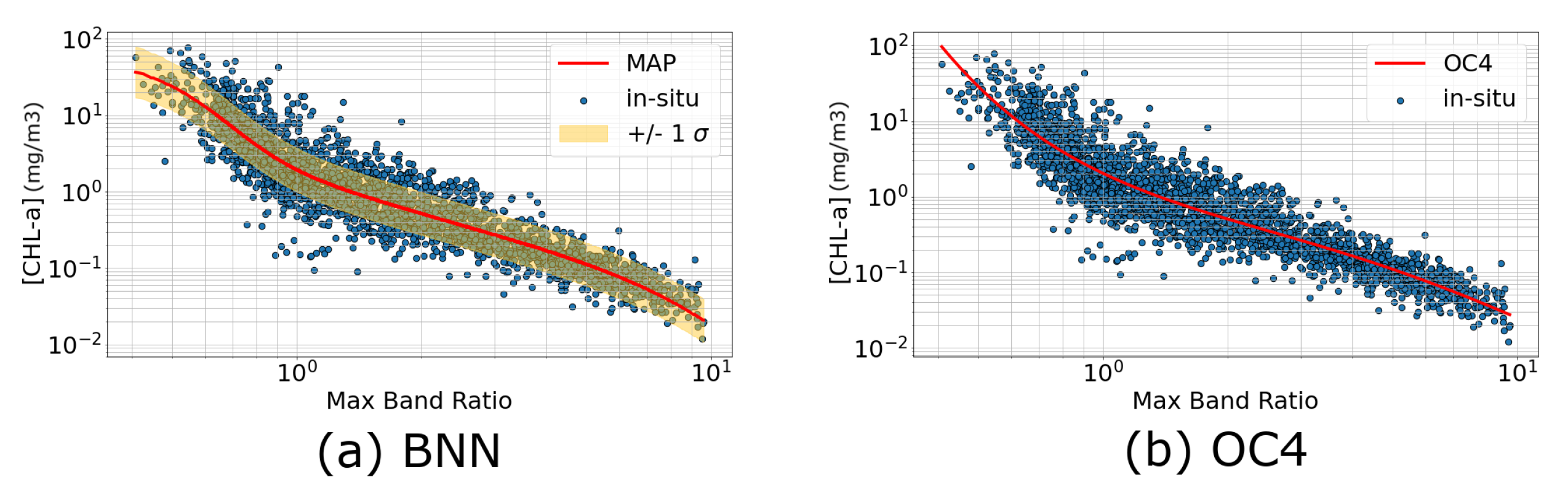
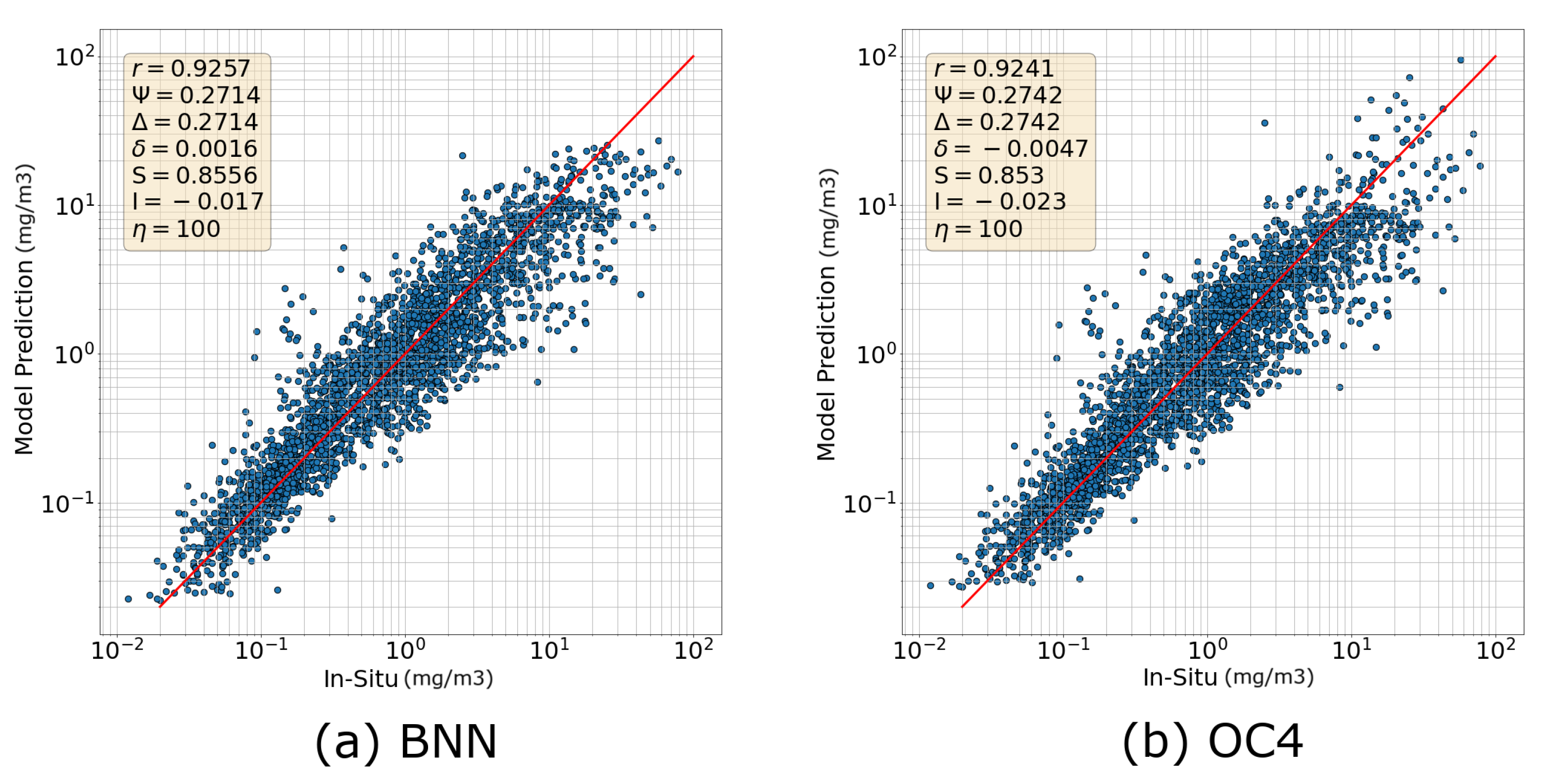
3.1.1. Comparison with OC4

The BNN MAP accurately captures the relationship between [CHL-a] and the MBR, indicating that higher MBR values correspond to lower [CHL-a] values (Figure 1). The uncertainties inherent to the match-ups are also adequately captured within the standard deviation range, where most of the in situ measurements are covered by this window. These results suggest that the BNN does not overfit to the dataset, behaving similarly to the OC4 model and adequately predicting [CHL-a] and its associated uncertainty. Furthermore, the BNN provides reliable estimates of the first two statistical moments, and its predictions fit the distribution of the data.

To assess the performance of the models, various statistical measures were computed and are presented in Figure 2. A strong correlation is observed between the model predictions and the in situ measurements for both the BNN and OC4 models, with r values of 0.9257 and 0.9241, respectively. This suggests that the BNN’s prediction with the highest probability performs at least as well as the OC4 when only MBR is used as input. Note that the BNN also allows for uncertainty estimates through an ensemble of predictions that characterize a posterior distribution for [CHL-a], which implies better characterization of the prediction’s reliability, which adds another layer of information to the analysis. The slope and intercept of a type II regression are close to 1 and 0, respectively, for both the BNN’s MAP ($S=0.8556$ and $I=-0.017$) and for OC4 ($S=0.853$ and $I=-0.023$). These measures suggest that the BNN’s highest probability prediction correlates with the data almost equally to OC4, while imposing a slightly smaller bias. The errors resulting from the BNN’s MAP ($\mathsf{\Psi }=0.2714$ and $\Delta =0.2714$) are also slightly smaller than those obtained with OC4 ($\mathsf{\Psi }=0.2742$ and $\Delta =0.2742$). Consequently, when only MBR from a single sensor is used as input, the BNN model performs similarly to OC4.

3.1.2. Comparison with OCI

There is a general positive agreement between both the MAP and OCI predictions with the in situ data, as seen from Figure 3a,b. Since the OC4 and OCI algorithms rely on reflectances from different wavelengths, the size of the dataset used for training these models is different. However, there are some points, primarily representing low [CHL-a] values, that are not captured well by the OCI model, as seen by the deviation of the OCI predictions (red) from the in situ values (blue) (Figure 3b). Figure 3c,d indicate a strong correlation between the MAP predictions and the in situ measurements with a correlation coefficient of $r=0.9155$, which is slightly higher than the correlation coefficient between the in situ and OCI predictions ($r=0.9126$). This suggests that the performance of the BNN’s highest probability predictions is similar to the OCI, with the added benefit of estimating the uncertainties associated with the prediction. Regarding other statistical measures, the OCI model performs slightly less favorably compared to the MAP and OC4 models. Specifically, the OCI model exhibits slightly larger MSEs ($\mathsf{\Psi }=0.3033$ and $\Delta =0.3021$) and a larger absolute bias ($\left|\delta \right|=0.0263$) than the BNN MAP ($\mathsf{\Psi }=0.2980$, $\Delta =0.2979$ and $\left|\delta \right|=0.003$). This signifies that the BNN’s MAP is more accurate than the OCI prediction, which exhibits a bias in its prediction that is an order of magnitude larger than that of the BNN’s MAP (Figure 3d). Therefore, the BNN performs slightly better than the OCI when using only the MBR from a single sensor as input.

3.1.3. Maximum Band Ratio from Multiple Sensors

The in situ match-ups from all satellites demonstrate a strong correlation, as depicted in Figure S1, illustrating the relationship between in situ [CHL-a] and MBR in the compiled database [41]. To capitalize on this comprehensive database, a BNN model was trained using the combined database comprised of the match-ups retrieved using MODIS, OLCA, OLCB, MERIS, SeaWIFS, and VIIRS, benefiting from a larger database than when using match-ups from a single satellite. Using the MBR definitions presented in [20] for the OC4 model, a BNN was trained using a comprehensive dataset involving matchups from MODIS, OLCA, OLCB, MERIS, SeaWIFS, and VIIRS.

The model realizations sampled from the BNN exhibit similar behavior with the MBR, with predictions exhibiting a wider spread at extreme MBR values and a tighter spread at the center where the in situ points are densely concentrated (Figure 4a). This suggests that any given BNN model realization will provide reliable estimates of [CHL-a] for MBR values that are not too small or too large, where data are abundant. However, the deviation in the predictions between different model realizations becomes significant for extreme MBR values, which corresponds to limited data regimes. Statistical measures demonstrate comparable error and correlation values to those obtained from the BNN trained on the SeaWiFS dataset (Figure 4b). Particularly, the MAP of the BNN trained on the combined dataset yields a high correlation coefficient $r=0.9159$, low errors with $\mathsf{\Psi }=0.2968$ and $\Delta =0.2963$, small bias $\delta =-0.017$, and reasonably reliable S and I values of 0.825 and –0.013, respectively. For comparison, Figure S2a,b present the OC4 predicted [CHL-a] as a function of the MBR and the corresponding scatter plot of the in situ [CHL-a] against their model-predicted counterparts. Consequently, when training the model with the MBR from multiple sensors, the BNN maintains high accuracy, similar to standard algorithms. This highlights the flexibility that the BNN offers, enabling the input of MBR from any combination of sensors without impacting its performance.

3.2. Advancing Beyond Standard Ocean Color Algorithm Capabilities

Standard ocean color algorithms rely on reflectances from specific wavelength bands in the green and blue spectrum to compute the MBR or $\xi$ to estimate [CHL-a]. A major advantage of the proposed framework is that it enables the use of one or multiple variables describing the ocean’s condition as additional input to the standard models without empirical tuning and with great implementation simplicity. This modeling flexibility enables data fusion of multi-modality datasets to exploit all available datasets describing the status of the ocean surface and atmosphere. Specifically, the input vector is extended to include auxiliary data co-located with the reflectance data. Initially, we train the BNN model using reflectances directly. Subsequently, we examine the addition of IOPs, coordinates, SST, and SST climatology to the previously described MBR-based model.

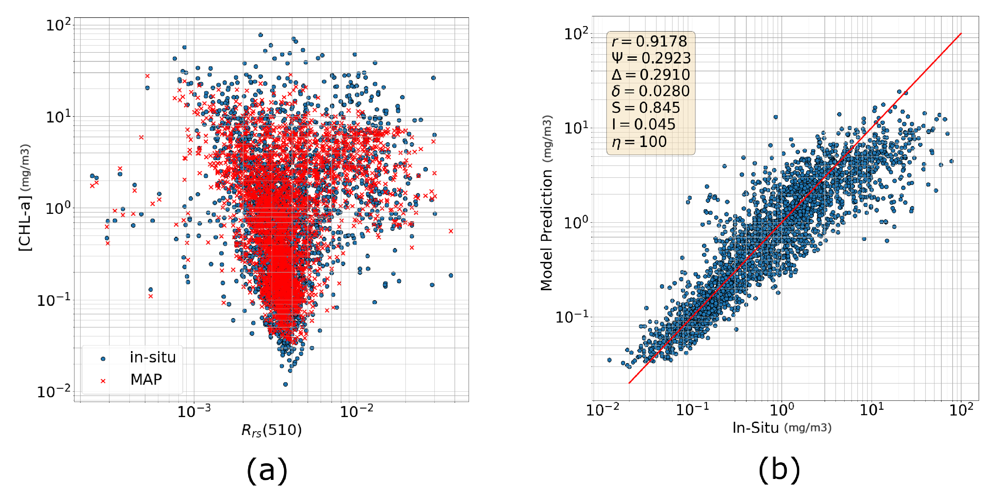
3.2.1. Training Directly with Reflectances

In this experiment, we explore the use of $R_{rs}$ in the blue and green wavelengths, instead of the MBR, as input for the BNN model to construct a higher-dimensional ocean color model. Specifically, we employ the SeaWiFS $R_{rs}$ at wavelengths of 411 nm, 443 nm, 489 nm, 510 nm, and 555 nm as inputs to the BNN to predict [CHL-a]. The scatter plot depicted in Figure 5a indicates a high correlation between the MAP predictions and the in situ measurements of [CHL-a] against the reflectances, where the reflectance value at 510 nm ($R_{rs}\left(510\right)$) was selected for illustration. The BNN’s MAP predictions follow the same distribution of [CHL-a] as the in situ data, with the points scattered within close proximity to each other, with the exception of some extreme values (Figure 5). A strong correlation exists between the in situ data points and their corresponding model predictions, as evidenced by the high correlation coefficient (r = 0.9178) and the S and I values of 0.845 and 0.045, respectively. Even though the resulting errors are relatively small ($\mathsf{\Psi }=0.2923$ and $\Delta =0.2910$), they are slightly larger compared to those obtained using the MBR model (Section 3.1.1).

3.2.2. Incorporating IOPs

IOPs are essential for gaining insights into the characteristics of seawater, providing valuable insights into the composition, [CHL-a], and distribution of optically active substances in the ocean, such as phytoplankton, suspended particles, and colored dissolved organic matter [73]. The inclusion of phytoplankton absorption coefficients is investigated, specifically $a_{ph}$ at wavelengths of 411 nm, 443 nm, 489 nm, 510 nm, and 555 nm, in conjunction with the MBR, as input to the BNN model. This BNN model was trained using the SeaWiFS dataset under the training conditions described in Section 2.3.

Figure 6a shows that the MAP’s [CHL-a] predictions closely follow the behavior of the in situ data. Notably, the inclusion of the absorption coefficient leads to a reduction in prediction uncertainty, as evidenced by the tighter clustering of data points and the improved statistical measures in comparison to the previous models (Figure 6). Particularly, a substantial correlation ($r=0.9628$) and Type-II regression slope close to 1 ($S=0.919$) are observed between the in situ measurements and the model predictions, which means that this model’s MAP predictions closely resemble the in situ values. Minimal errors are also observed, where $\mathsf{\Psi }=0.1665$ and $\Delta =0.1664$, the lowest among all explored models. The MAP also yields a low bias of $\left|\delta \right|=0.0069$ and intercept $I=-0.02$, comparable to those obtained with the MBR model in Section 3.1.1. These results suggest that including IOPs, when they are available, offers more reliable MAP predictions with around $40\%$ lower error than relying solely on MBR as input.

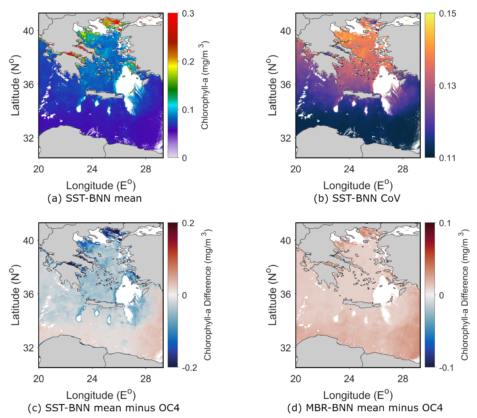
3.2.3. Incorporating Coordinates and Sea Surface Temperature

A major advantage of the proposed AI framework is that it enables the use of multiple variables describing the ocean’s condition as input to the model, such as the SST, which is an important variable for phytoplankton growth. To investigate the impact of including SST on the performance of the BNN, the matchups database was extended to incorporate SST, SST climatological means, and the spatial coordinates (longitude and latitude) as additional inputs to the MBR-based BNN model. While SST is an important factor for phytoplankton growth, it slightly improves upon the model’s performance, whereas information about the location and SST climatology significantly improved prediction reliability. This suggests that phytoplankton growth can be affected differently by SST variations in each region.

Again, there is a clear agreement between the BNN’s MAP predictions and the in situ observations (Figure 7). Moreover, predictions no longer fit a single curve as with the predictions in Section 3.1.1 and Section 3.1.2, where adding more variables as input introduces new dimensions to the prediction, allowing it to capture deviations that were previously unachievable. This BNN model achieves high correlation values with $r=0.9455$, and a significant reduction of ∼20% in $\mathsf{\Psi }$ and $\Delta$ in comparison to the models in Section 3.1.1 and Section 3.1.2. This indicates that using a nonlinear combination of the remotely sensed reflectances achieves significantly better accuracy than combining these reflectances into the MBR. Furthermore, the slope and intercept of a Type-II regression are $S=0.829$ and $I=-0.026$, indicating good correlation and low bias for the MAP predictions with respect to the in situ data. These results highlight the significance of incorporating additional variables describing oceanic conditions to enhance the performance of ocean color models.

4. Spatial Evaluation of the BNN Models

In this section, [CHL-a] estimates from OC4, the MBR-based BNN model (MBR-BNN), and the best performing BNN model (SST-BNN) are compared spatially. The MBR-based BNN model and OC4 use the same input variables for [CHL-a] estimation, while the SST-BNN model also includes coordinates, SST, and SST climatology. Comparisons are made at different spatial and temporal resolutions, using daily Sentinel-3 imagery, as well as monthly AQUA-MODIS imagery. We identify potential model performance disparities across different marine ecosystems by conducting the comparison over a diverse range of regions and environmental conditions, including distinct coastal and open ocean areas. In addition to comparing the average BNN model predictions to those of OC4, the coefficient of variation (CoV) is presented as a normalized measure of the magnitude of uncertainty. Due to the large difference between mean [CHL-a] values in the selected regions, the CoV is a more suitable metric than standard deviation (StD) alone, since it is normalized by the mean, giving a relative estimate of the confidence in the prediction. The CoV is defined as the ratio of the StD to the mean of the ensemble of the BNN sample predictions, which was computed using the logarithmic [CHL-a] predictions. This is particularly significant because the BNN predicted distributions are heteroskedastic, meaning that the StD varies with the mean value. In other words, lower CoV values indicate that the StD is low compared to the mean; thus, the predictions are more reliable, while the opposite is true for higher CoV values.

4.1. Sentinel-3 Daily Imagery

Single scenes of two regions with different environmental conditions and typical [CHL-a] phenology during different seasons were selected for the spatial comparison of the three different models: the Aegean Sea (Figure 8) and the Southern Red Sea (SRS) including the Gulf of Aden (Figure 9). In all these cases, Sentinel-3 daily images were used to estimate an ensemble of [CHL-a] realizations, from which the mean and CoV were computed and reported. The Aegean Sea, located in the Eastern Mediterranean Sea, is characterized by a temperate climate and generally low [CHL-a]. The SRS is a tropical sea with many shallow regions populated by coral reefs, where [CHL-a] variability is much higher. Furthermore, the training dataset contains many more points from the Mediterranean Sea compared to the Red Sea, allowing us to investigate whether it has an effect on the model predictions. The mean and CoV of both BNN model predictions are calculated from 100 different samples generated from unique model realizations, which is a reasonable tradeoff between storage requirements and resolution.

4.1.1. Aegean Sea

The Aegean Sea scene was taken on the 23rd of May 2020 and is characterized by a relatively low [CHL-a] that increases slightly from South to North, reaching its highest values near the coasts. Figure 8a shows that the very low [CHL-a] values have the lowest CoV values due to their very low StD, while the highest CoV is observed at [CHL-a] values between 0.1 and 0.2 mg/m³ (Figure 8b). The highest [CHL-a] values, predominantly close to the coasts, have a relatively low StD in comparison to the mean, which translates into low CoV. This suggests that the model predictions are more reliable in the Southern Aegean than the Northern Aegean, where uncertainty is slightly higher. Consequently, confidence in the model prediction is lower in those areas.

Some differences can be observed between the SST-BNN prediction mean values and the OC4 estimates (Figure 8c). The SST-BNN predicts slightly higher [CHL-a] at the very low concentrations (<0.08 mg/m³), while the OC4 estimates much higher [CHL-a] at the highest concentrations (>0.2 mg/m³) near the coasts. This suggests that the SST-BNN predictions are more conservative in regions with high [CHL-a], which is due to the network architecture. The standard ocean color algorithms, such as OC4, are also known to overestimate [CHL-a] in such regions, especially near the coasts. On the other hand, the differences between the average MBR-BNN prediction and the OC4 estimate are relatively small (Figure 8d). This is an expected result, since both models use the same input variables (MBR). An overall slight negative bias is also present in the OC4 estimate compared to the MBR-BNN mean prediction.

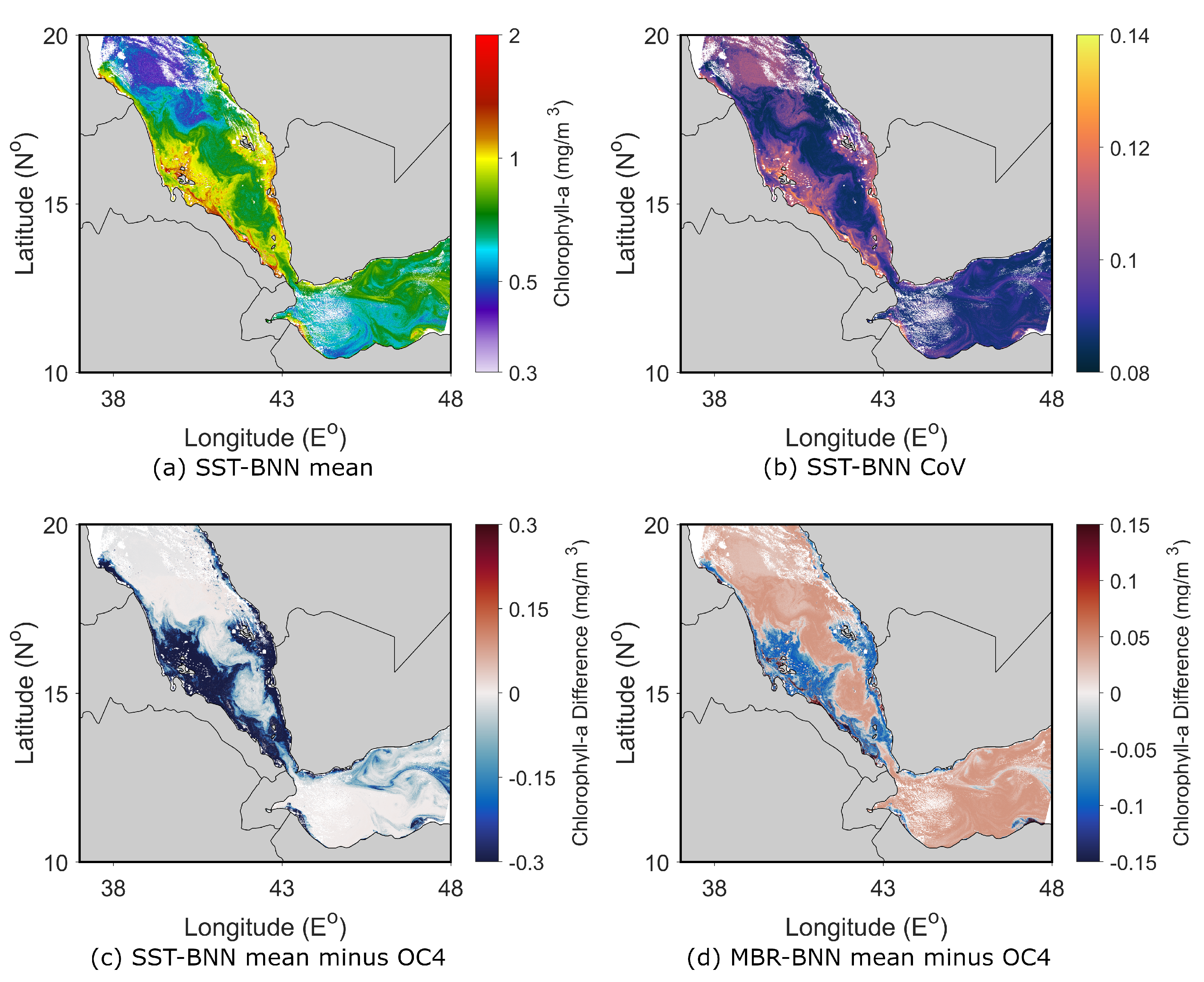
4.1.2. Southern Red Sea

The SRS scene was taken on the 20th of November 2019 and shows a much larger spatial variability in [CHL-a] than the Aegean Sea (Figure 9a). The SRS is relatively shallow and is characterized by higher [CHL-a] than the central Red Sea and the Gulf of Aden. The CoV (Figure 9b) is slightly smaller than that obtained in the Aegean, which is likely associated with the larger mean [CHL-a] in the SRS in comparison to the Aegean Sea. Specifically, the CoV is smallest in productive open ocean areas, where the mean [CHL-a] values are between 0.6 and 0.9 mg/m³, and largest in shallower coastal areas, which are typically associated with high [CHL-a] concentrations (>1 mg/m³). It is also worth noting that the lack of training data from the Red Sea did not increase the CoV, indicating that the SST-BNN can be used effectively on a global scale.

There are more evident differences between the three models in the SRS than in the Aegean Sea. Similarly, the average SST-BNN predicts lower [CHL-a] in the most productive and some of the coastal areas compared to the OC4 estimation (Figure 9c). On the other hand, their difference is negligible in most of the lower concentration open sea areas of the SRS and the Gulf of Aden. As was the case in the Aegean Sea image, the MBR-BNN mean prediction is similar to the OC4 estimate due it to sharing the same input variables (Figure 9d). However, there are areas that the OC4 slightly overestimates compared to the MBR-BNN model: the high productivity areas. Such areas appear to be the most susceptible to overestimation by the standard ocean color algorithms, such as the OC4, since, even with the same input variables, the MBR-BNN mean values are still lower.

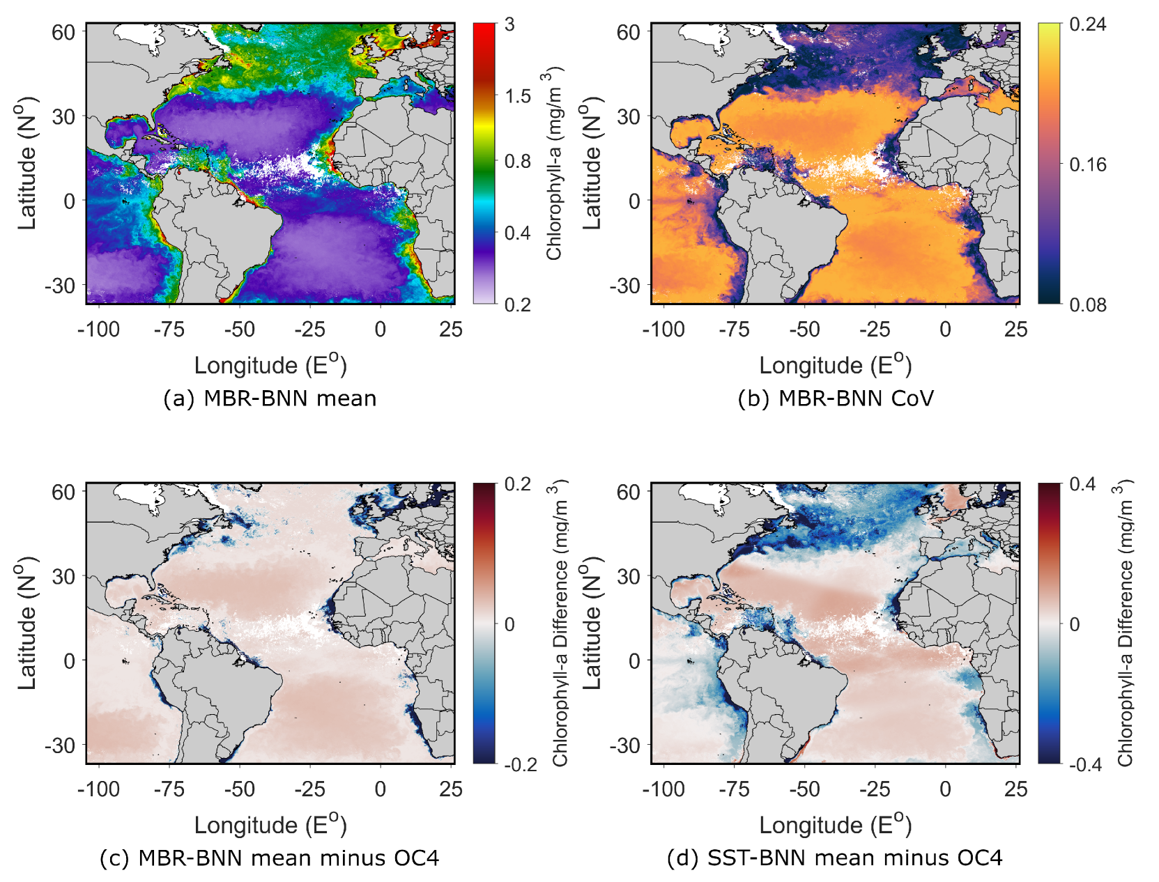
4.2. MODIS Monthly Imagery

A global monthly composite image was retrieved from MODIS for May of 2009 and used to analyze the performances of the MBR-BNN and SST-BNN models in comparison to that of OC4. The SST-BNN model was designed to take the SST at a given instance as input to the model, whereas a composite employs average quantities as input. Therefore, the MBR-BNN is used as the optimal model in this case since it is more suitable for dealing with composite images. Note that the comparison thereon is among the predictions performed on the same MODIS composite scene. During May, as expected, the MBR-BNN mean [CHL-a] is high in the northern Atlantic Ocean, the Baltic Sea, and in most of the coastal regions of South America and Western Africa (Figure 10a). Due to the higher mean values, the CoV of these areas (~0.1) is lower than the open sea areas (~0.2) that have lower mean [CHL-a] values, such as the oceanic waters between −30 and 30 N°. Consequently, the MBR-BNN’s predictions are more certain in higher concentration regions, such as the coast and the northern regions.

The differences between both BNN models and the OC4 algorithm follow a similar pattern (Figure 10c,d). Similarly to the Sentinel-3 daily images discussed above, the BNN models predict lower [CHL-a] values in high productivity areas and slightly lower [CHL-a] values in low productivity areas. These differences have a larger magnitude between the SST-BNN mean predictions and the OC4 estimates, which arise from using the monthly mean SST as input. Even though the MBR-BNN demonstrates that it can be conveniently used to predict [CHL-a] from composite imagery, the highest accuracy would be achieved by using daily data as input to the SST-BNN, then averaging the predictions for a given period.

5. Limitations and Future Directions

As with all computational tools, there are limitations in the tool’s use in certain settings. One of the limitations of including additional datasets in the BNN training is the difference in spatial resolution amongst different data modalities. For instance, while Sentinel-3 imagery is available at around 300 × 300 m resolution, the OSTIA SST dataset is available at 0.05° resolution, meaning that errors associated with regridding the data onto the same mesh will inevitably arise. Additionally, each data modality that is used for training the BNN model must be used as input for predicting [CHL-a]; i.e., all the input variables must be available to use the model. In some cases, this could limit the applicability of the trained BNN model, or even training in the case when an adequate number of matchups cannot be achieved. Monthly composites of MBR and SST (or any other dataset) also offer a significant limitation, where by definition, the SST-BNN requires instantaneous SST estimates as input, not averages. While the MBR-BNN can still be used in those cases, the SST-BNN should be used to predict [CHL-a] with daily data and then average those to create temporal means. Nevertheless, these limitations do not hinder the utility of the BNN model in various applications requiring rigorous understanding of the uncertainty associated with [CHL-a].

There are several applications and directions for future work. The proposed methodology can be used for policy making by estimating quantities such as probability at risk, where the probability of eutrophication events can be estimated, leading to more informed environmental protection strategies. Along the same lines, the probability distribution output from the proposed model can be used to monitor extreme events. For instance, the conditional probability that [CHL-a] exceeds a certain threshold can be monitored as an early detection strategy for extreme events. Furthermore, tuning BNN models with more high-quality regional observations would further improve the model’s reliability in regions with higher prediction uncertainty. Such regionally tuned BNN models could also be tailored to offer predictions at higher accuracies for specific ecoregions.

6. Conclusions

This work introduces the use of a Bayesian Neural Network (BNN) for estimating chlorophyll-a ([CHL-a]) from remotely sensed data, using the largest available database of in situ match-ups. The BNN’s MAP performs at a slightly higher accuracy than established ocean color models, such as OC4 and OCI, providing reliable estimates for [CHL-a] when the same inputs are used. The learning-based method also allows for more degrees of freedom in ocean color modeling by involving more input variables, describing the state of the ocean, to more reliably predict the [CHL-a] concentration. Specifically, when an extended input vector, including data such as coordinates and SST, is used for estimating the surface [CHL-a], the prediction errors with respect to the in situ values are reduced by 20–40% compared to standard ocean color algorithms (Table 1). The potential of the BNN model also lies in its uncertainty quantification capabilities, where the BNN predicts the distribution of potential [CHL-a] values, which builds confidence in the predicted values and enables further statistical analyses.

By including uncertainty estimates, the proposed model provides additional information that is missing from traditional algorithms. This is especially beneficial for coastal waters when using higher spatial resolution ocean color imagery, such as from the Sentinel-3 OLCI. This could benefit coastal ecosystem health and biodiversity assessments by studying the nutrient circulation, detecting localized HABs, as well as monitoring climate change and other anthropogenic impacts on phytoplankton dynamics. While the BNN may not guarantee more accurate results in challenging regions in comparison to their deterministic counterparts, they offer a means of estimating uncertainties indicating when it lacks confidence in its predictions. These uncertainty estimates help us to understand when and where the BNN predictions are reliable, as opposed to other regions where uncertainties are large and additional data may be necessary to improve prediction accuracy. In addition to enabling enhanced management applications, the proposed BNN models also offer new directions for research in the field of ocean color remote sensing, such as region-specific models.

Table 1. Summary of the percentage relative error in statistical measures for each of the algorithms relative to the NASA Ocean Chlorophyll 4-band (OC4) model, calculated as $100\times (x_{alg}-x_{oc4})/x_{oc4}$, where x is a statistical measure, and the subscript corresponds to the algorithm. The algorithms listed are as follows: BNN based on the maximum band ratio of SeaWiFS (BNN-MBR), Ocean Color Index (OCI), BNN based on the three wavelengths used by the OCI algorithm (BNN-OCI), BNN based on the maximum band ratio from multiple sensors (BNN-MBR merged), BNN based on five reflectance values from SeaWiFS (BNN-Rrs), BNN based on absorption coefficient $a_{ph}$ (BNN-abs), BNN based on the maximum band ratio, spatial coordinates, and sea surface temperature (BNN-enhanced). Higher correlation, lower errors, and bias are preferred. The row italicized indicates the best model in terms of errors and correlation. The row highlighted in bold font indicates the best performing model based on readily available auxiliary data, including the SST and geospatial coordinates.

	r	Ψ	Δ	δ
OC4	-	-	-	-
BNN-MBR	0.173	−1.021	−1.021	−134.043
OCI	−1.244	10.613	10.175	−659.574
BNN-OCI	−0.931	8.680	8.643	−36.170
BNN-MBR (merged dataset)	−0.887	8.242	8.060	261.702
BNN-Rrs	−0.682	6.601	6.127	−695.745
BNN-abs	4.188	−39.278	−39.314	46.809
BNN-enhanced	2.316	−12.874	−12.874	−4.255

Table 1. Summary of the percentage relative error in statistical measures for each of the algorithms relative to the NASA Ocean Chlorophyll 4-band (OC4) model, calculated as $100\times (x_{alg}-x_{oc4})/x_{oc4}$, where x is a statistical measure, and the subscript corresponds to the algorithm. The algorithms listed are as follows: BNN based on the maximum band ratio of SeaWiFS (BNN-MBR), Ocean Color Index (OCI), BNN based on the three wavelengths used by the OCI algorithm (BNN-OCI), BNN based on the maximum band ratio from multiple sensors (BNN-MBR merged), BNN based on five reflectance values from SeaWiFS (BNN-Rrs), BNN based on absorption coefficient $a_{ph}$ (BNN-abs), BNN based on the maximum band ratio, spatial coordinates, and sea surface temperature (BNN-enhanced). Higher correlation, lower errors, and bias are preferred. The row italicized indicates the best model in terms of errors and correlation. The row highlighted in bold font indicates the best performing model based on readily available auxiliary data, including the SST and geospatial coordinates.

	r	Ψ	Δ	δ
OC4	-	-	-	-
BNN-MBR	0.173	−1.021	−1.021	−134.043
OCI	−1.244	10.613	10.175	−659.574
BNN-OCI	−0.931	8.680	8.643	−36.170
BNN-MBR (merged dataset)	−0.887	8.242	8.060	261.702
BNN-Rrs	−0.682	6.601	6.127	−695.745
BNN-abs	4.188	−39.278	−39.314	46.809
BNN-enhanced	2.316	−12.874	−12.874	−4.255

References

1. Harris, G. Phytoplankton Ecology: Structure, Function and Fluctuation; Springer Science & Business Media: Berlin/Heidelberg, Germany, 2012. [Google Scholar]
2. Jones, R.I. Phytoplankton, primary production and nutrient cycling. In Aquatic Humic Substances: Ecology and Biogeochemistry; Springer: Berlin/Heidelberg, Germany, 1998; pp. 145–175. [Google Scholar]
3. Falkowski, P.G.; Raven, J.A. Aquatic Photosynthesis; Princeton University Press: Princeton, NJ, USA, 2013. [Google Scholar]
4. Hays, G.C.; Richardson, A.J.; Robinson, C. Climate change and marine plankton. Trends Ecol. Evol. 2005, 20, 337–344. [Google Scholar] [CrossRef] [PubMed]
5. Haeder, D.P.; Villafane, V.E.; Helbling, E.W. Productivity of aquatic primary producers under global climate change. Photochem. Photobiol. Sci. 2014, 13, 1370–1392. [Google Scholar] [CrossRef] [PubMed]
6. Basu, S.; Mackey, K.R. Phytoplankton as key mediators of the biological carbon pump: Their responses to a changing climate. Sustainability 2018, 10, 869. [Google Scholar] [CrossRef]
7. Platt, T.; Fuentes-Yaco, C.; Frank, K.T. Spring algal bloom and larval fish survival. Nature 2003, 423, 398–399. [Google Scholar] [CrossRef]
8. Anderson, D.M.; Glibert, P.M.; Burkholder, J.M. Harmful algal blooms and eutrophication: Nutrient sources, composition, and consequences. Estuaries 2002, 25, 704–726. [Google Scholar] [CrossRef]
9. Gokul, E.A.; Raitsos, D.E.; Gittings, J.A.; Alkawri, A.; Hoteit, I. Remotely sensing harmful algal blooms in the Red Sea. PLoS ONE 2019, 14, e0215463. [Google Scholar] [CrossRef]
10. Klemas, V. Remote sensing of algal blooms: An overview with case studies. J. Coast. Res. 2012, 28, 34–43. [Google Scholar] [CrossRef]
11. Racault, M.F.; Platt, T.; Sathyendranath, S.; Ağirbaş, E.; Martinez Vicente, V.; Brewin, R. Plankton indicators and ocean observing systems: Support to the marine ecosystem state assessment. J. Plankton Res. 2014, 36, 621–629. [Google Scholar] [CrossRef]
12. Platt, T.; White III, G.N.; Zhai, L.; Sathyendranath, S.; Roy, S. The phenology of phytoplankton blooms: Ecosystem indicators from remote sensing. Ecol. Model. 2009, 220, 3057–3069. [Google Scholar] [CrossRef]
13. Hazen, E.L.; Suryan, R.M.; Santora, J.A.; Bograd, S.J.; Watanuki, Y.; Wilson, R.P. Scales and mechanisms of marine hotspot formation. Mar. Ecol. Prog. Ser. 2013, 487, 177–183. [Google Scholar] [CrossRef]
14. Racault, M.F.; Le Quéré, C.; Buitenhuis, E.; Sathyendranath, S.; Platt, T. Phytoplankton phenology in the global ocean. Ecol. Indic. 2012, 14, 152–163. [Google Scholar] [CrossRef]
15. Shu, C.; Xiu, P.; Xing, X.; Qiu, G.; Ma, W.; Brewin, R.J.; Ciavatta, S. Biogeochemical Model Optimization by Using Satellite-Derived Phytoplankton Functional Type Data and BGC-Argo Observations in the Northern South China Sea. Remote Sens. 2022, 14, 1297. [Google Scholar] [CrossRef]
16. Joint, I.; Groom, S.B. Estimation of phytoplankton production from space: Current status and future potential of satellite remote sensing. J. Exp. Mar. Biol. Ecol. 2000, 250, 233–255. [Google Scholar] [CrossRef] [PubMed]
17. Morel, A.; Prieur, L. Analysis of variations in ocean color1. Limnol. Oceanogr. 1977, 22, 709–722. [Google Scholar] [CrossRef]
18. Bricaud, A.; Babin, M.; Morel, A.; Claustre, H. Variability in the chlorophyll-specific absorption coefficients of natural phytoplankton: Analysis and parameterization. J. Geophys. Res. Ocean. 1995, 100, 13321–13332. [Google Scholar] [CrossRef]
19. Groom, S.; Sathyendranath, S.; Ban, Y.; Bernard, S.; Brewin, R.; Brotas, V.; Brockmann, C.; Chauhan, P.; Choi, J.k.; Chuprin, A.; et al. Satellite ocean colour: Current status and future perspective. Front. Mar. Sci. 2019, 6, 485. [Google Scholar] [CrossRef] [PubMed]
20. O’Reilly, J.E.; Werdell, P.J. Chlorophyll algorithms for ocean color sensors—OC4, OC5 & OC6. Remote Sens. Environ. 2019, 229, 32–47. [Google Scholar]
21. Mélin, F. Uncertainties in Ocean Colour Remote Sensing; International Ocean Colour Coordinating Group (IOCCG): Dartmouth, NS, Canada, 2019. [Google Scholar] [CrossRef]
22. Neil, C.; Spyrakos, E.; Hunter, P.D.; Tyler, A.N. A global approach for chlorophyll-a retrieval across optically complex inland waters based on optical water types. Remote Sens. Environ. 2019, 229, 159–178. [Google Scholar] [CrossRef]
23. Doerffer, R.; Schiller, H. The MERIS Case 2 water algorithm. Int. J. Remote Sens. 2007, 28, 517–535. [Google Scholar] [CrossRef]
24. Yu, B.; Xu, L.; Peng, J.; Hu, Z.; Wong, A. Global chlorophyll-a concentration estimation from moderate resolution imaging spectroradiometer using convolutional neural networks. J. Appl. Remote Sens. 2020, 14, 034520. [Google Scholar] [CrossRef]
25. Ye, H.; Tang, S.; Yang, C. Deep learning for Chlorophyll-a concentration retrieval: A case study for the Pearl River Estuary. Remote Sens. 2021, 13, 3717. [Google Scholar] [CrossRef]
26. Fan, D.; He, H.; Wang, R.; Zeng, Y.; Fu, B.; Xiong, Y.; Liu, L.; Xu, Y.; Gao, E. CHLNET: A novel hybrid 1D CNN-SVR algorithm for estimating ocean surface chlorophyll-a. Front. Mar. Sci. 2022, 9, 934536. [Google Scholar] [CrossRef]
27. Hadjal, M.; Medina-Lopez, E.; Ren, J.; Gallego, A.; McKee, D. An artificial neural network algorithm to retrieve chlorophyll a for Northwest European shelf seas from top of atmosphere ocean colour reflectance. Remote Sens. 2022, 14, 3353. [Google Scholar] [CrossRef]
28. MacKay, D.J. Bayesian neural networks and density networks. Nucl. Instruments Methods Phys. Res. Sect. A Accel. Spectrometers Detect. Assoc. Equip. 1995, 354, 73–80. [Google Scholar] [CrossRef]
29. Jospin, L.V.; Laga, H.; Boussaid, F.; Buntine, W.; Bennamoun, M. Hands-On Bayesian Neural Networks—A Tutorial for Deep Learning Users. IEEE Comput. Intell. Mag. 2022, 17, 29–48. [Google Scholar] [CrossRef]
30. Shen, G.; Chen, X.; Deng, Z. Variational Learning of Bayesian Neural Networks via Bayesian Dark Knowledge. In Proceedings of the Twenty-Ninth International Joint Conference on Artificial Intelligence, IJCAI-20; Bessiere, C., Ed.; International Joint Conferences on Artificial Intelligence Organization: Montreal, QC, Canada, 2020; pp. 2037–2043. [Google Scholar] [CrossRef]
31. Izmailov, P.; Vikram, S.; Hoffman, M.D.; Wilson, A.G.G. What Are Bayesian Neural Network Posteriors Really Like? In Proceedings of the 38th International Conference on Machine Learning, Virtual, 18–24 July 2021; Meila, M., Zhang, T., Eds.; Proceedings of Machine Learning Research. Volume 139, pp. 4629–4640. [Google Scholar]
32. Magris, M.; Iosifidis, A. Bayesian learning for neural networks: An algorithmic survey. Artif. Intell. Rev. 2023, 56, 11773–11823. [Google Scholar] [CrossRef]
33. Kendall, A.; Gal, Y. What Uncertainties Do We Need in Bayesian Deep Learning for Computer Vision? In Proceedings of the Advances in Neural Information Processing Systems; Guyon, I., Luxburg, U.V., Bengio, S., Wallach, H., Fergus, R., Vishwanathan, S., Garnett, R., Eds.; Curran Associates, Inc.: Newry, UK, 2017; Volume 30. [Google Scholar]
34. Goan, E.; Fookes, C. Bayesian Neural Networks: An Introduction and Survey. In Case Studies in Applied Bayesian Data Science: CIRM Jean-Morlet Chair, Fall 2018; Mengersen, K.L., Pudlo, P., Robert, C.P., Eds.; Springer International Publishing: Cham, Switzerland, 2020; pp. 45–87. [Google Scholar] [CrossRef]
35. Chen, B.; Zhang, A.; Cao, L. Autonomous intelligent decision-making system based on Bayesian SOM neural network for robot soccer. Neurocomputing 2014, 128, 447–458. [Google Scholar] [CrossRef]
36. Abdullah, A.A.; Hassan, M.M.; Mustafa, Y.T. A Review on Bayesian Deep Learning in Healthcare: Applications and Challenges. IEEE Access 2022, 10, 36538–36562. [Google Scholar] [CrossRef]
37. Pahlevan, N.; Smith, B.; Schalles, J.; Binding, C.; Cao, Z.; Ma, R.; Alikas, K.; Kangro, K.; Gurlin, D.; Ha, N.; et al. Seamless retrievals of chlorophyll-a from Sentinel-2 (MSI) and Sentinel-3 (OLCI) in inland and coastal waters: A machine-learning approach. Remote Sens. Environ. 2020, 240, 111604. [Google Scholar] [CrossRef]
38. Saranathan, A.M.; Smith, B.; Pahlevan, N. Per-Pixel Uncertainty Quantification and Reporting for Satellite-Derived Chlorophyll-a Estimates via Mixture Density Networks. IEEE Trans. Geosci. Remote Sens. 2023, 61, 4200718. [Google Scholar] [CrossRef]
39. Saranathan, A.M.; Werther, M.; Balasubramanian, S.V.; Odermatt, D.; Pahlevan, N. Assessment of advanced neural networks for the dual estimation of water quality indicators and their uncertainties. Front. Remote Sens. 2024, 5, 1383147. [Google Scholar] [CrossRef]
40. Frouin, R.; Pelletier, B. Bayesian methodology for inverting satellite ocean-color data. Remote Sens. Environ. 2015, 159, 332–360. [Google Scholar] [CrossRef]
41. Valente, A.; Sathyendranath, S.; Brotas, V.; Groom, S.; Grant, M.; Jackson, T.; Chuprin, A.; Taberner, M.; Airs, R.; Antoine, D.; et al. A compilation of global bio-optical in situ data for ocean colour satellite applications–version three. Earth Syst. Sci. Data 2022, 14, 5737–5770. [Google Scholar] [CrossRef]
42. Werdell, P.; Bailey, S. The SeaWiFS Bio-Optical Archive and Storage System (SeaBASS): Current Architecture and Implementation; Technical Memorandum 2002-211617; NASA Goddard Space Flight Center: Greenbelt, MD, USA, 2002. [Google Scholar]
43. Werdell, P.J.; Bailey, S.W. An improved in-situ bio-optical data set for ocean color algorithm development and satellite data product validation. Remote Sens. Environ. 2005, 98, 122–140. [Google Scholar] [CrossRef]
44. Barker, K.; Mazeran, C.; Lerebourg, C.; Bouvet, M.; Antoine, D.; Ondrusek, M.; Zibordi, G.; Lavender, S. Mermaid: The MERIS matchup in-situ database. In Proceedings of the 2nd (A) ATSR and MERIS Workshop, Frascati, Italy, 22–26 September 2008; pp. 22–26. [Google Scholar]
45. Matrai, P.; Olson, E.; Suttles, S.; Hill, V.; Codispoti, L.; Light, B.; Steele, M. Synthesis of primary production in the Arctic Ocean: I. Surface waters, 1954–2007. Prog. Oceanogr. 2013, 110, 93–106. [Google Scholar] [CrossRef]
46. Devine, L.; Galbraith, P.S.; Joly, P.; Plourde, S.; Saint-Amand; Pierre, J.S.; Starr, M. Chemical and Biological Oceanographic Conditions in the Estuary and Gulf of St. Lawrence During 2015; Fisheries and Oceans Canada, Ecosystems and Oceans Science: Sidney, BC, Canada, 2015. [Google Scholar]
47. Nechad, B.; Ruddick, K.; Schroeder, T.; Oubelkheir, K.; Blondeau-Patissier, D.; Cherukuru, N.; Brando, V.; Dekker, A.; Clementson, L.; Banks, A.C.; et al. CoastColour Round Robin data sets: A database to evaluate the performance of algorithms for the retrieval of water quality parameters in coastal waters. Earth Syst. Sci. Data 2015, 7, 319–348. [Google Scholar] [CrossRef]
48. Peloquin, J.M.; Swan, C.; Gruber, N.; Vogt, M.; Claustre, H.; Ras, J.; Uitz, J.; Barlow, R.G.; Behrenfeld, M.J.; Bidigare, R.R.; et al. The MAREDAT global database of high performance liquid chromatography marine pigment measurements - Gridded data product (NetCDF) - Contribution to the MAREDAT World Ocean Atlas of Plankton Functional Types. Earth Syst. Sci. Data 2013, 5, 109–123. [Google Scholar] [CrossRef]
49. Clark, D.; Murphy, M.; Yarbrough, M.; Feinholz, M.; Flora, S.; Broenkow, W.; Johnson, B.; Brown, S.; Kim, Y.; Mueller, J. MOBY, A Radiometric Buoy for Performance Monitoring and Vicarious Calibration of Satellite Ocean Color Sensors: Measurement and Data Analysis Protocols. 2003. Available online: https://ntrs.nasa.gov/api/citations/20030063145/downloads/20030063145.pdf (accessed on 19 May 2025).
50. Stark, J.D.; Donlon, C.J.; Martin, M.J.; McCulloch, M.E. OSTIA: An operational, high resolution, real time, global sea surface temperature analysis system. In Proceedings of the OCEANS 2007-Europe, Aberdeen, UK, 18–21 June 2007; pp. 1–4. [Google Scholar] [CrossRef]
51. Donlon, C.; Berruti, B.; Buongiorno, A.; Ferreira, M.H.; Féménias, P.; Frerick, J.; Goryl, P.; Klein, U.; Laur, H.; Mavrocordatos, C.; et al. The Global Monitoring for Environment and Security (GMES) Sentinel-3 mission. Remote Sens. Environ. 2012, 120, 37–57. [Google Scholar] [CrossRef]
52. O’Reilly, J.; Maritorena, S.; Siegel, D.; O’Brien, M.; Toole, D.; Mitchell, B.; Kahru, M.; Chavez, F.; Strutton, P.; Cota, G. Ocean Color Chlorophyll a Algorithms for SeaWiFS, OC2, and OC4: Technical Report; SeaWiFS Postlaunch Technical Report Series; SeaWiFS Postlaunch Calibration and Validation Analyses Part 3; NASA, Goddard Space Flight Center: Greenbelt, MD, USA, 2000; Volume 11. [Google Scholar]
53. Hammoud, M.A.E.R.; Mittal, H.V.R.; Le Maître, O.; Hoteit, I.; Knio, O. Variance-based sensitivity analysis of oil spill predictions in the Red Sea region. Front. Mar. Sci. 2023, 10, 1185106. [Google Scholar] [CrossRef]
54. Hu, C.; Lee, Z.; Franz, B. Chlorophyll aalgorithms for oligotrophic oceans: A novel approach based on three-band reflectance difference. J. Geophys. Res. Ocean. 2012, 117. [Google Scholar] [CrossRef]
55. Brewin, R.J.; Sathyendranath, S.; Müller, D.; Brockmann, C.; Deschamps, P.Y.; Devred, E.; Doerffer, R.; Fomferra, N.; Franz, B.; Grant, M.; et al. The Ocean Colour Climate Change Initiative: III. A round-robin comparison on in-water bio-optical algorithms. Remote Sens. Environ. 2015, 162, 271–294. [Google Scholar] [CrossRef]
56. Neal, R.M. Bayesian Learning for Neural Networks; Springer: New York, NY, USA, 1996. [Google Scholar] [CrossRef]
57. Bingham, E.; Chen, J.P.; Jankowiak, M.; Obermeyer, F.; Pradhan, N.; Karaletsos, T.; Singh, R.; Szerlip, P.; Horsfall, P.; Goodman, N.D. Pyro: Deep Universal Probabilistic Programming. J. Mach. Learn. Res. 2019, 20, 973–978. [Google Scholar] [CrossRef]
58. Samaniego, F.J. A comparison of the Bayesian and Frequentist Approaches to Estimation; Springer: New York, NY, USA, 2010; Volume 24. [Google Scholar]
59. Chen, T.; Chen, H. Universal approximation to nonlinear operators by neural networks with arbitrary activation functions and its application to dynamical systems. IEEE Trans. Neural Netw. 1995, 6, 911–917. [Google Scholar] [CrossRef] [PubMed]
60. Moore, T.S.; Campbell, J.W.; Dowell, M.D. A class-based approach to characterizing and mapping the uncertainty of the MODIS ocean chlorophyll product. Remote Sens. Environ. 2009, 113, 2424–2430. [Google Scholar] [CrossRef]
61. Blei, D.M.; Kucukelbir, A.; McAuliffe, J.D. Variational Inference: A Review for Statisticians. J. Am. Stat. Assoc. 2017, 112, 859–877. [Google Scholar] [CrossRef]
62. Hoffman, M.D.; Blei, D.M.; Wang, C.; Paisley, J. Stochastic variational inference. J. Mach. Learn. Res. 2013, 14, 1303–1347. [Google Scholar]
63. Ranganath, R.; Gerrish, S.; Blei, D. Black box variational inference. In Proceedings of the Artificial Intelligence and Statistics, Reykjavik, Iceland, 22–25 April 2014; pp. 814–822. [Google Scholar]
64. Kingma, D.P.; Welling, M. Auto-Encoding Variational Bayes. arXiv 2022, arXiv:1312.6114. [Google Scholar]
65. Olivier, A.; Shields, M.D.; Graham-Brady, L. Bayesian neural networks for uncertainty quantification in data-driven materials modeling. Comput. Methods Appl. Mech. Eng. 2021, 386, 114079. [Google Scholar] [CrossRef]
66. Li, D.; Marshall, L.; Liang, Z.; Sharma, A.; Zhou, Y. Bayesian LSTM with Stochastic Variational Inference for Estimating Model Uncertainty in Process-Based Hydrological Models. Water Resour. Res. 2021, 57, e2021WR029772. [Google Scholar] [CrossRef]
67. Campagne, J.E.; Lanusse, F.; Zuntz, J.; Boucaud, A.; Casas, S.; Karamanis, M.; Kirkby, D.; Lanzieri, D.; Peel, A.; Li, Y. JAX-COSMO: An End-to-End Differentiable and GPU Accelerated Cosmology Library. Open J. Astrophys. 2023, 6. [Google Scholar] [CrossRef]
68. Kingma, D.P.; Ba, J. Adam: A Method for Stochastic Optimization. arXiv 2017, arXiv:1412.6980. [Google Scholar]
69. Bishop, C.M. Pattern Recognition and Machine Learning; Springer: New York, NY, USA, 2006. [Google Scholar]
70. Ben Hammouda, C.; Ben Rached, N.; Tempone, R. Importance sampling for a robust and efficient multilevel Monte Carlo estimator for stochastic reaction networks. Stat. Comput. 2020, 30, 1665–1689. [Google Scholar] [CrossRef]
71. Bishop, C.M. Mixture Density Networks; Technical Report NCRG/94/004; Aston University: Birmingham, UK, 1994. [Google Scholar]
72. Gal, Y.; Ghahramani, Z. Dropout as a Bayesian Approximation: Representing Model Uncertainty in Deep Learning. In Proceedings of the 33rd International Conference on Machine Learning, New York, NY, USA, 20–22 June 2016; pp. 1050–1059. [Google Scholar]
73. Woźniak, S.B.; Meler, J.; Stoń-Egiert, J. Inherent optical properties of suspended particulate matter in the southern Baltic Sea in relation to the concentration, composition and characteristics of the particle size distribution; new forms of multicomponent parameterizations of optical properties. J. Mar. Syst. 2022, 229, 103720. [Google Scholar] [CrossRef]
Figure 1. Scatter plots illustrating the [CHL-a] for the in situ (blue dots), (a) BNN’s MAP prediction (red), and uncertainties represented by ± σ (shaded in yellow) for a BNN trained using the SeaWiFS dataset and (b) the OC4 prediction (red) as a function of the MBR.
Remotesensing 17 01826 g001
Figure 2. Scatter plots for the in situ [CHL-a] as a function of the (a) BNN’s MAP and (b) OC4. The scatter plots are accompanied with the resulting error statistics. The plot shows the metrics comparing the MAP and OC4 predictions with the reference measurements. Indicated are the Pearson correlation coefficient (r), root mean squared error ( Ψ ), unbiased root mean squared error ( Δ ), retrieval percentage ( η ), slope (S), intercept (I) of a Type-II regression, and the bias ( δ ).
Remotesensing 17 01826 g002
Figure 3. (a,b) Scatter plots illustrating the [CHL-a] for the in situ values (blue dots), (a) BNN’s MAP prediction (red) (b) the OCI prediction (red) as a function of the MBR, and (c,d) scatter plot of the in situ [CHL-a] as a function of the corresponding model predictions for the BNN’s MAP and OCI models, respectively.
Remotesensing 17 01826 g003
Figure 4. (a) Plot illustrating [CHL-a] curves as a function of MBR for 50 randomly sampled BNN models (colored curves) and the in situ data points. (b) Scatter plot showing the in situ [CHL-a] measurements against the MAP predictions for a BNN trained using the combined dataset.
Remotesensing 17 01826 g004
Figure 5. (a) Scatter plot of the [CHL-a] against R r s ( 510 ) for the in situ measurements and the MAP predictions. (b) Scatter plot illustrating the in situ [CHL-a] measurements against their corresponding MAP predictions.
Remotesensing 17 01826 g005
Figure 6. (a) 3D scatter plot illustrating a projection of the [CHL-a] along the MBR and a p h ( 411 ) for the in situ measurements and MAP predictions. (b) Scatter plot of the measured in situ [CHL-a] as a function of the MAP predictions with the resulting statistical measures.
Remotesensing 17 01826 g006
Figure 7. (a) Scatter plot illustrating a projection of the [CHL-a] along the MBR for the in situ measurements and MAP predictions. (b) Scatter plot of the measured in situ [CHL-a] as a function of the MAP predictions with the resulting statistical measures.
Remotesensing 17 01826 g007
Figure 8. A single scene of the Aegean Sea from Sentinel-3 at ~300 m spatial resolution depicting: (a) the average [CHL-a] field obtained from the SST-BNN model, (b) the Coefficient of Variation (CoV) of the SST-BNN predictions, (c) the difference between the SST-BNN mean and the OC4 [CHL-a] estimation, and (d) the difference between the MBR-BNN mean and the OC4 [CHL-a] estimation.
Remotesensing 17 01826 g008
Figure 9. A single scene of the southern Red Sea from Sentinel-3 at ~300 m spatial resolution depicting: (a) the average [CHL-a] field obtained from the SST-BNN model, (b) the Coefficient of Variation (CoV) of the SST-BNN predictions, (c) the difference between the SST-BNN mean and the OC4 [CHL-a] estimation, and (d) the difference between the MBR-BNN mean and the OC4 [CHL-a] estimation.
Remotesensing 17 01826 g009
Figure 10. A single scene of the southern Red Sea from Sentinel-3 at ~300 m spatial resolution depicting: (a) the average [CHL-a] field obtained from the MBR-BNN model, (b) the Coefficient of Variation (CoV) of the MBR-BNN predictions, (c) the difference between the MBR-BNN mean and the OC4 [CHL-a] estimation, and (d) the difference between the SST-BNN mean and the OC4 [CHL-a] estimation.
Remotesensing 17 01826 g010
Disclaimer/Publisher’s Note: The statements, opinions and data contained in all publications are solely those of the individual author(s) and contributor(s) and not of MDPI and/or the editor(s). MDPI and/or the editor(s) disclaim responsibility for any injury to people or property resulting from any ideas, methods, instructions or products referred to in the content.