Snow Cover Trends in the Chilean Andes Derived from 39 Years of Landsat Data and a Projection for the Year 2050

Abstract

Snow cover is an important freshwater source in many mountain ranges around the world and is heavily affected by climate change, often leading to reduced overall snow cover availability and duration as well as shifts in seasonality. To monitor these changes and long-term trends, the analysis of remote sensing is a commonly used tool, as data are available consistently and for long time series. In this study we acquired and processed the whole archive of available Landsat data between 1985 and 2024 for two catchments in the Chilean Andes, Aconcagua and Río Maipo, located in the Valparaíso and Santiago de Chile metropolitan regions, respectively. We generated monthly Snow Line Elevation (SLE) time series from the entire archive for both catchments and performed trend analyses on these time series. Strong positive long-term SLE change rates of 11.25 m per year for the Aconcagua catchment and 9.85 m to 15.65 m per year for the Río Maipo catchment were detected, indicating a decrease in snow cover as well as available freshwater from snowmelt. The projection to the year 2050 revealed a potential loss of snow covered area of up to 42% during summer months, with the SLE receding up to 231 m.

1. Introduction

Santiago de Chile, the capital of the country, has experienced an exponential growth in population and economy during the last years. In total, 7.1 million people out of 17.5 million people in Chile are living in the metropolitan region of the capital of Chile [1]. Water from snow and ice melt in the Andes Mountain range is one of the most important contributors to water supply for irrigation, industries, and hydro-power generation in this region [2]. The Andes are often referred to as a “water tower”, providing the main source of freshwater for Chile. Recent studies of retreating glaciers and snow cover reveal the fragile future of the freshwater supply for the population of central Chile (33–37°S) [3]. Mid-tropospheric warming in the central Andes increases the fraction of precipitation that falls as rain rather than snow, leading to earlier melting and peaks in river runoff [4]. This can result in flooding in winter and spring, followed by water shortages in late spring and summer [5]. In addition to climate change, El Niño and La Niña can also play a crucial role in the amount and extent of snowfall in the Andes Mountains. While the effect is generally bigger in the northern regions, the area around the metropolitan region of Santiago de Chile is influenced by such events as well [6], introducing more uncertainty into the prediction of future developments. Reliable estimations of these future snow cover dynamics are, however, of the highest importance for policy- and decision-makers, planners, and other stakeholders in Chile.

In remote, high-altitude mountain regions, spaceborne Earth observation (EO) plays a crucial role in acquiring snow cover information. While Bormann et al. [7] pointed out the limited potential of medium-resolution remote sensing data (namely, MODIS) to quantify long-term trends of snow cover in mountain areas [8], we claim that the higher-resolution Landsat data provide the potential to detect trends and analyze Snow Line Elevation (SLE) dynamics in high-altitude mountain ranges. The spatial resolution of 30 m is precise enough to capture the complex processes in mountainous regions [9] while the long time series of available data (since the mid-1980s) is sufficient to derive possible trends. This potential was already demonstrated by Koehler et al. [10] for the European Alps and Wang et al. for the Himalayas [11].

Several studies about the snow and glacier development in the Andes have been conducted in the past: Cordero et al. [12] calculated snow cover extents for 22 zones in the Andes using Landsat data from 1986 to 2018 and a binary classification scheme based on a single threshold for NDSI data. Snow cover was found to decline at an average rate of about −12% per decade across the entire study area. Saavedra et al. [13,14] identified snow climate regions by elevation and timing of snow accumulation based on the MODIS binary snow cover product, a promising approach based on the time series of a snow cover index, and documented an elevation change of the snowline of 10–30 m per year south of 29–30° using the 8-days MODIS snow product. Hanshaw et al. [15] calculated the time series of glacial areas, lakes, and snow lines in the Andes from 1975 to 2012 by using a multi-step classification scheme based on Landsat data. They reported serious difficulties in delineating snow lines and therefore implemented a spectral mixture analysis with the endmembers snow, ice, and shadow. A Landsat-based glacier study from Bolivia highlighted the importance of both precipitation and temperature patterns for the SLE. The authors concluded that a general rising trend of the SLE is visible from the data, but because of the short time series, with the study being conducted in 2001, the results are not significant [16].

Nonetheless, no study has yet approached the question of how the snow cover dynamics around the metropolitan region of Santiago de Chile have changed on a catchment basis while relying on a Landsat-based snow classification together with a Digital Elevation Model (DEM) to retrieve Snow Line Elevation time series. Our approach has the advantage of being able to estimate SLE also during partly clouded conditions, increasing data availability considerably.

In this context, the main objectives of this study are as follows:

• Derive multi-decadal time series of SLE dynamics from Landsat data, starting from 1985;
• Calculate SLE trends for the major catchments of central Chile, including SLE anomalies on a monthly and seasonal basis; SLE trends on a seasonal basis, especially for the dry season (January through March; JFM) and for October and November, where runoff from snowmelt is greatest and runoff from glacier melt at its minimum;
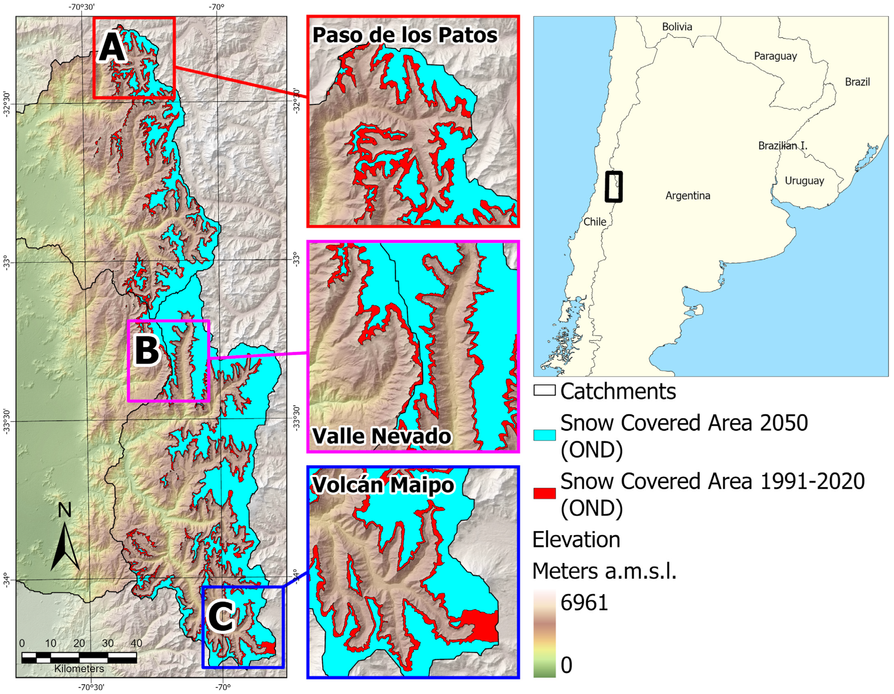
• Project the evolution of the SLE based on the derived trends for the potential SLE situation in the year 2050 and determine whether remote sensing-based data and methods can be used to predict small-scale developments and changes of the cryosphere in the Andes Mountains.

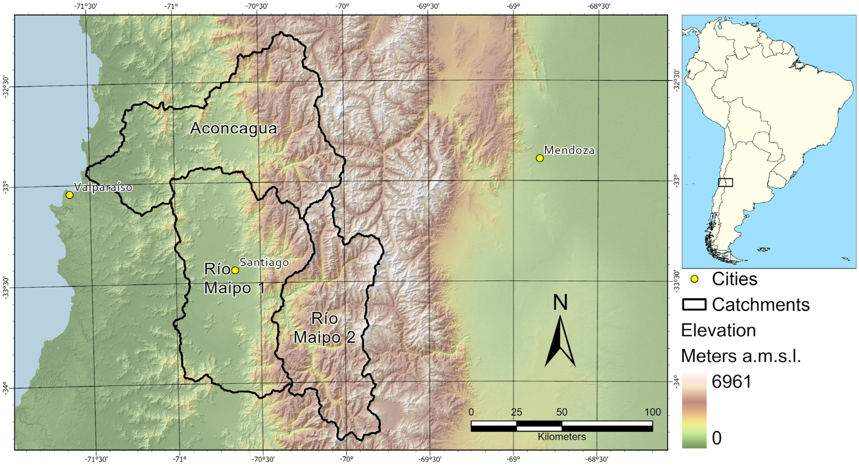
The presented study showcases the successful application of the SLE method to the Andes Mountains, a region where it had not been previously applied. Building on its proven efficacy in the Carpathian Mountains [17] and European Alps [10,18], this study breaks new ground by deriving SLE statistics seasonally for the first time. This innovative approach provides more nuanced insights into the impact of climate change on the development of seasonal snow cover, revealing distinct seasonal trends.

2. Study Area

With Aconcagua and Río Maipo, the two most relevant catchments for the water supply of Valparaiso and Santiago de Chile, respectively, have been selected as study areas. These two catchments are situated in the western Main Cordillera east of the metropolitan region of Santiago de Chile in the Mediterranean central Chile. Details about the investigated catchments are summarized in

Table 1. Statistics of investigated catchments. Glaciated area derived from the GLIMS Glacier database. Río Maipo has been divided into a western part (Río Maipo 1) and an eastern part (Río Maipo 2) due to Landsat tile coverage.

River Catchment	Total Area [km2]	Max. Elevation [m a.s.l.]	Glaciated Area [km2]	Long-Term Median SLE July [m a.s.l.]
Aconcagua	7 322	5 748	46	2410
Maipo-1: west	6 998	5 193	6	2136
Maipo-2: east	4 838	6 961	360	2020

. Both catchments are W-E-oriented and reach elevations from sea level to 6961 m a.s.l (above sea level). SLE is known to decrease strongly with latitude [13,19]. Considering the entire Andes, the SLE decreases from 5000 m a.s.l. at 10°S to 700 m a.s.l. at 38°S [13]. The day of year with the lowest SLE is usually in July for the metropolitan region of Santiago de Chile, with an elevation of 2018 m ± 725 m [13]. At this latitude (34°S), differences in SLE between the eastern and western sides of the Andes are most pronounced because the mountains are particularly high, and the orographic effects on local precipitation decrease further south, where elevations do not reach such high values. North-facing, wind-sheltered slopes were found to have lower snow accumulation than south-facing, wind-exposed hillslopes, suggesting that the radiation budget is more important than wind transport [20].

The vegetation in the study region is limited to geomorphologically stable areas below ~3200 m a.s.l. [21] and consists of shrubs and small trees adapted to dry conditions in lower elevations, which transition into grasses, mosses, and lichens in high-elevation zones. The 0 °C isotherm altitude of mean air temperature is estimated at 3600 m a.s.l. [22].

2.1. Aconcagua Catchment

The Aconcagua River is located at the boundary between semi-arid and central Chile. The river basin has a total area of 7 322 km² [23]. Ohlanders et al. [24] have shown, for a sub-catchment of the Aconcagua catchment (Juncal Basin), that glacier melt is the dominant source of streamflow at times of high discharge. Snowmelt is dominant during spring (mid-October to mid-November), which makes these months especially interesting to our study. Trend analysis of streamflow at several stations in the Aconcagua basin has revealed a significant decreasing trend for the period from 1970 to 2002 [25,26]. In contrast to streamflow, precipitation did not show a decreasing trend, suggesting that the decrease in streamflow during this period was due to changes in glacier volume and area.

2.2. Río Maipo Catchment

With Santiago de Chile in the center, the Río Maipo river basin is the most populated region of Chile. For the Río Maipo catchment, we calculated SLE dynamics for two sub-basins (Río Maipo 1 in the west and Río Maipo 2 in the east), partially due to the reason that the Río Maipo catchment is covered by two adjacent Landsat tiles, leading to shifted observation dates. An overview of the study site and the location of the catchments is available in Figure 1.

2.3. Climate

In central Chile, summers are dry and precipitation—mainly of frontal and orographic origin—concentrates on winter months. During summer months, precipitation is low due to the blocking of a high-pressure cell over the south-east Pacific Ocean [27], while runoff is at its maximum during the same months [28]. On average, most precipitation occurs between May and August, with 62% of the total precipitation occurring during the winter months (June through August; JJA). During the summer months (December through February; DJF) precipitation is less than 2% of the annual sum [26].

The metropolitan region of Santiago de Chile experiences great interannual variability of precipitations due to large-scale modes such as the El Niño-Southern Oscillation (ENSO) and Southern Annular Mode (SAM). As indicated in the introduction, El Niño and La Niña can have a significant impact on the amount of snowfall, particularly in the northern regions of the Andes [6]. Cordero et al. [12] have shown that changes in El Niño account for most of the Andean snow cover losses, as El Niño determines Sea Surface Temperature (SST) anomalies, resulting in altered precipitation regimes. The decline in snow cover is more pronounced on the western side of the Andes than on the eastern side [12,14]. Rainfall shows positive anomalies during the developing stage of warm events of the Southern Oscillation, while cold events correspond to dry conditions [27].

Between 1975 and 2001, the central Andes experienced an air temperature increase of approximately 0.25 °C per decade [29]. This temperature rise caused the 0 °C isotherm to shift upward by about 120 m in winter and roughly 200 m in summer between 30° and 38°S, as reported by Carrasco et al. [30]. Central Chile has been severely affected by a so-called megadrought since 2010 [31,32], with reduced snowfall altering water supply to its headwaters. Corripio et al. [28] have modeled SST increase impacts on the Aconcagua catchments and found that runoff during the ablation season is likely to decrease in the future after a short period of enhanced runoff due to effects caused by glacier melt. At the same time, winter precipitation will not increase, depleting ice rapidly and leading to an overall decrease in the glaciated area.

3. Materials and Methods

For the metropolitan region of Santiago de Chile, we generated time series of Snow Line Elevation (SLE) for the Aconcagua and Río Maipo catchments. Utilizing a modified approach based on Hu et al. [18], and further refined by Koehler et al. [10] for large-scale applications, we computed SLE values from Landsat data spanning nearly four decades (1985–2024). To ensure data quality, the SLE observations underwent a reliability filtering process, followed by a resampling to obtain monthly means. Any data gaps were subsequently filled using linear interpolation, resulting in a continuous and evenly spaced time series of monthly SLE observations.

3.1. Data

Our analysis leveraged the Landsat sensor family, which provided a unique opportunity to generate extensive time series of Snow Line Elevation (SLE) observations. A key strength of Landsat data lies in its exceptional continuity, with regular and comparable acquisitions dating back to 1985. The Landsat constellation offers a revisit time of 16 days, which is further enhanced during periods when multiple Landsat sensors are operational, thereby increasing the temporal resolution. This enables a detailed understanding of intra-annual dynamics. With a spatial resolution of up to 30 m for multispectral bands, Landsat makes a detailed mapping of land surface features possible, even in complex and fragmented mountainous regions. Furthermore, Landsat’s multispectral capabilities encompass not only visible wavelengths but also near-infrared and short-wave infrared (SWIR) bands. Additionally, the thermal sensor, with a resolution of 60 m, proves particularly valuable for distinguishing between snow and clouds, a crucial aspect of SLE monitoring.

To optimize processing efficiency, we utilized Landsat Collection 2 Level-2 Tier 1 Surface Reflectance (SR) products, which offer atmospherically and topographically corrected reflectance values. These corrections enable seamless comparability across multiple Landsat sensors, facilitating robust time series analysis [33]. The study area was covered by six Landsat tiles, encompassing acquisition paths 232, 233, and 234, with data provided by the United States Geological Survey (USGS). In total, we processed 5261 scenes, with each tile contributing between 1041 and 1069 scenes. Notably, data coverage increased in recent years due to the concurrent operation of multiple Landsat sensors. We chose not to apply a cloud cover threshold for data exclusion, as the SLE is derived at the catchment level, which typically constitutes a subset of the entire scene and may be less affected by cloud cover. Moreover, as a statistical measure, the SLE can be estimated from a relatively small subset of data, albeit with reduced reliability [10].

For the extraction of the SLE from Landsat-based snow classifications, we employed the Copernicus Global Digital Elevation Model (DEM) as our topographic reference. Specifically, we utilized the GLO-30 variant, which provides a spatial resolution of one arc-second, corresponding to the 30 m resolution of the Landsat data [34]. Given the significance of snow as a hydrological parameter, we selected river catchments as the primary spatial unit of analysis for SLE calculation. To define these catchments, we leveraged the HydroBASINS dataset, a product of the HydroSHEDS project [23], which provides a comprehensive and standardized framework for hydrological analysis.

3.2. Snow Classification

As suggested by Hu et al. [18] and validated for the entire Alps region by Koehler et al. [10], we utilized a threshold-based snow classification methodology. This approach integrates a temperature and shadow thresholding strategy as outlined by the Satellite Snow Product Intercomparison and Evaluation Exercise (SnowPEx) [35] and an index-based thresholding scheme originally designed for MODIS [36,37,38]. In this methodology, potential snow pixels are identified through a decision tree that examines thresholds in the green and near-infrared (NIR) spectral bands, as well as spectral indices including the normalized difference snow index (NDSI) [39] and the normalized difference vegetation index (NDVI) [37,40]. The subsequent application of several masks refines the snow classification: A temperature mask for values exceeding 288 K excludes pixels with temperatures too high for snow occurrence, while a combination of the normalized difference water index (NDWI > 0) [41] and reflectance in the visible green band (<0.2) delineates water bodies. Additionally, a combination of low values in the short-wave infrared (SWIR, <0.02), green (<0.2), and NDVI (<0.1) identifies topographical shadows. Finally, a cloud mask based on the FMASK algorithm [42] is applied. The binary cloud mask is generated from the pixel quality bands within the SR data. The NDSI, derived from the green and SWIR bands, plays a pivotal role in snow classification but is subject to limitations under certain conditions, such as the presence of water bodies and dense forests, which can result in false classification. To mitigate these limitations, we introduced a normalized difference between the blue and NIR bands to the classification scheme, enhancing the ability to differentiate snow from sunlit rock, bare soil, water, and clouds. The resultant classification encompasses the categories “clear land”, “snow”, “clouds”, “water/shadow”, and “no data”.

The efficiency of the classification scheme was previously assessed in the Alps using validation polygons on Landsat, Sentinel-2 imagery, and the Google Satellite Base Map in Google Earth Engine [10], where it demonstrated overall accuracy values of 87.5% (Landsat 5), 95.5% (Landsat 7), and 94.5% (Landsat 8). In addition, we performed an accuracy assessment of the Landsat snow classifications, relying on Sentinel-2 snow cover data retrieved through the Sen2Cor routine [43]. This assessment comprised 23 Sentinel-2 scenes after 2015, containing less than 50% clouds as well as a reasonable (at least 10%) percentage of snow-covered ground, and matching the Landsat observation date. This accuracy assessment revealed an overall accuracy of 96.84%. An exemplary map showing the Sentinal-2 comparison with Landsat is illustrated in the Supplementary Material (Figure S1). The confusion matrix resulting from the comparison of all 23 Sentinel-2–Landsat pairs is attached as Table S1.

3.3. Snow Line Elevation Retrieval and Time Series Generation

Using snow classifications based on data from Landsat and the Copernicus DEM, the SLE was calculated for each observation on a catchment basis. We applied a method originally developed by Krajcí et al. [17], who derived the SLE for a catchment in the Carpathian Mountains from daily MODIS data over the period 2000–2013. They defined the SLE as the elevation at which the sum of snow-covered pixels below and snow-free pixels above can be minimized. This method was adapted for use in the Alps with Landsat data by Hu et al. [18], who described the SLE as a statistical measure that can be calculated using the minimum of the two cumulative histograms of “snow” and “clear land” pixels. This approach enables SLE estimation even in cloudy conditions if there are enough sample pixels available [17]. To assess the accuracy and reliability of the SLE estimation, several quality indices were calculated for each derived SLE. We used the Representativeness Index (RI) to evaluate the number of valid pixels (i.e., “snow” and “clear land”) available for the SLE estimation. The Root Mean Square Error (RMSE) provided a measure of the accuracy of the derived snow line by calculating the distance of falsely classified pixels (i.e., “snow” below the SLE, “clear land” above the SLE) from the estimated SLE. The Error Index (EI) [18] was used to calculate the proportion of these erroneous pixels.

For the subsequent trend analyses, a time series with a regular observation frequency was required. First, we filtered the derived SLEs based on their quality. SLEs derived from images with an RI of less than 0.2 were rejected, as well as SLEs outside the elevation range of each catchment, as determined by the DEM. The remaining observations were then aggregated to monthly mean values to create a time series with regular time intervals. Any remaining data gaps were filled using linear interpolation. The time series was truncated to start in January 1985 (January 1990 for Río Maipo-2, as there was no Landsat data available before that time) and end in December 2023, resulting in a time series comprising 468 SLE estimations for each catchment, which served as the foundation for the following analyses.

We applied the two-sided seasonal Mann–Kendall test [44] to evaluate the significance of any long-term trends within the time series and used the seasonal Theil–Sen estimator [45] to calculate annual change rates. For the analysis of seasonal dynamics, the three SLE observations within a season were aggregated by their mean. Anomalies were calculated by subtracting each seasonal SLE observation from the respective seasonal median, which was calculated for a 30-year reference period (1991–2020). We chose to calculate the median for the long-term reference period instead of the mean to minimize the impact of outliers that sometimes occur during extreme years. The seasonal trends were calculated using the conventional (non-seasonal) variants of the Mann–Kendall test and Theil–Sen estimator, as they represent yearly values. The SLE value for the year 2050 was extrapolated based on the linear seasonal trends, using the reference period as a baseline for comparison. The snow cover area and its change percentage were calculated from the area above the derived and extrapolated SLE of the DEM.

4. Results

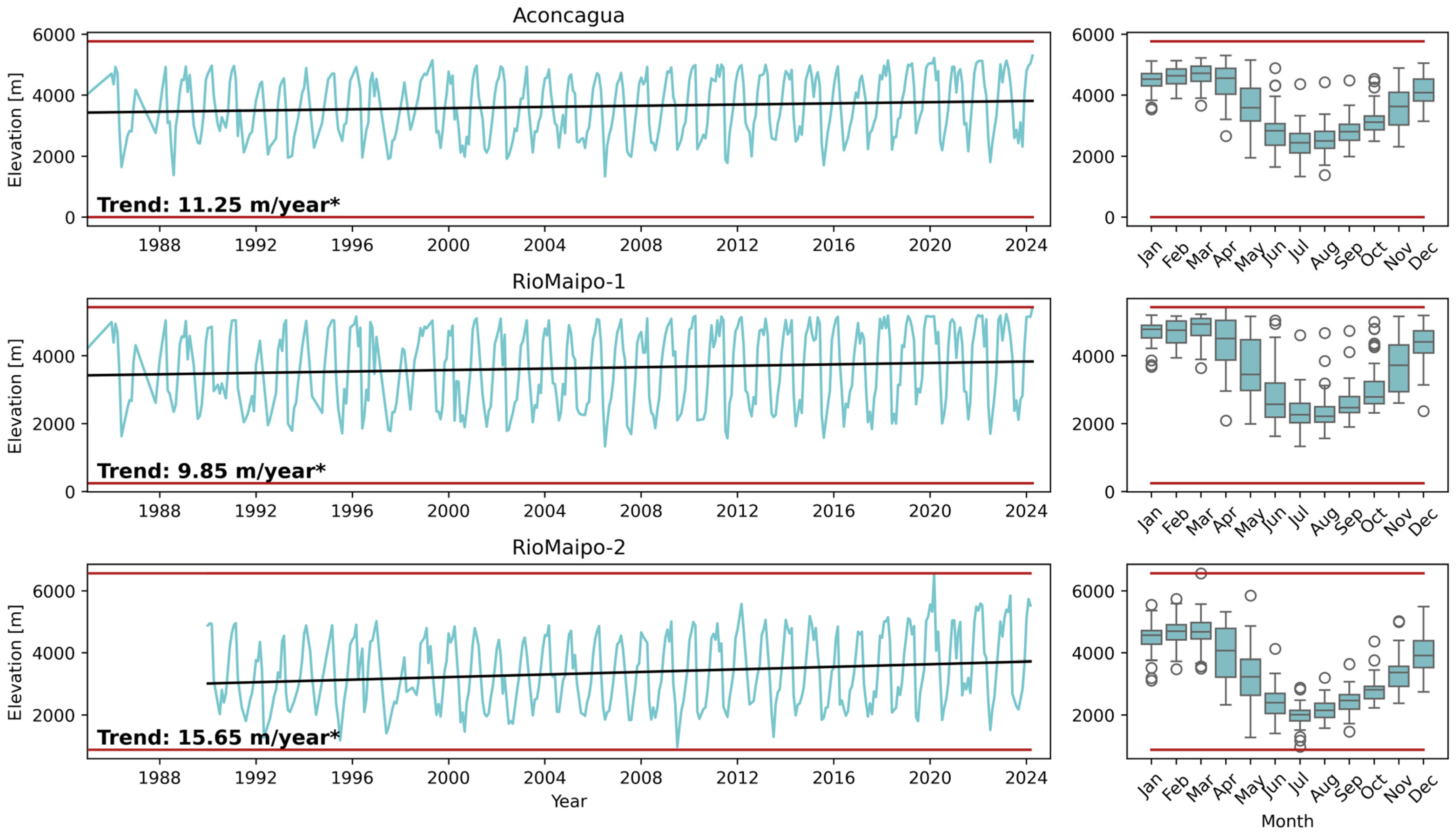
4.1. Properties of the SLE Time Series and Long-Term Dynamics

In addition to the SLE values for each catchment, quality indicators were derived from the Landsat-based snow classifications. Figure 2 illustrates the distributions of RI, EI, and RMSE. More than 80% of the derived SLEs were estimated on at least 52% of available clear-sky pixels, with the median RI located at 0.76. The number of incorrectly classified pixels (i.e., “snow” below the estimated SLE and “clear land” above the SLE) was low, with a median EI of 0.012, and the 80th percentile was 0.017. The median accuracy of the estimated SLE as measured by the RMSE was 453 m.

After applying the quality thresholds to the data, between 76% and 92% of all observations remained. The remaining observations were then aggregated to monthly mean SLE to generate regular, evenly spaced time series. The time series for the investigated catchments are illustrated in Figure 3 and exhibit the expected seasonal patterns, with low SLE in winter months and high elevations in summer. All catchments experienced a significant (p < 0.01) positive SLE change during the observation period, with the strongest trend in the eastern part of the Río Maipo catchment (Río Maipo-2, 15.65 m/y), followed by Aconcagua (11.25 m/y) and the western part of the Río Maipo catchment Río (Maipo-1, 9.85 m/y). The highest Snow Line Elevations typically occur during the dry season in summer in January, February, and March (JFM), while the lowest SLE occurs in winter in July, August, and September (JAS). Inter-annual variations of the SLE are usually more pronounced in the transitional months between summer and winter. Here, snowfall and snow melt contribute to a high dynamic of the SLE. Positive and negative outliers, however, have been observed in every month.

The positive trends of the SLE are reflected in the SLE anomalies from the long-term median (Figure 4). Positive SLE anomalies, i.e., less snow cover, have become more frequent since 2010. Anomalies tend to be more pronounced in spring and fall. However, a long period of positive SLE anomalies was also recorded during the dry season in the upper (2) Río Maipo catchment. Overall, positive SLE anomalies are generally more pronounced than negative anomalies and can exceed the long-term median by up to 2000 m a.s.l. Note that particularly strong anomalies in the early years of the time series may be due to the limited availability of suitable satellite observations and interpolation.

4.2. Seasonal SLE Trends and Extrapolation

Significant SLE trends are prevalent in the dry period in summer and the melting season in spring (Figure 5). The strongest trend in summer is observed in the eastern part of the Río Maipo catchment (Río Maipo-2) with a yearly change rate of 7.69 m, followed by the Aconcagua (4.80 m/y) and the western part of the Río Maipo catchment (Rio Maipo-1, 4.31 m/y). In spring, the strongest trend is observed in the western part of the Río Maipo catchment (Río Maipo 1) with 8.17 m/y, followed by Aconcagua (5.85 m/y). Although the change rate in the eastern part of theRío Maipo catchment (Rio Maipo-2) is quite high (6.17 m/y), it did not pass the significance test. No significant trends were detected for the fall and winter seasons in any catchment, even though the trend slopes might suggest otherwise. Note that compared to the trend analysis of the full time series, the trends calculated on a seasonal basis are less likely to surpass the significance threshold since the reduced amount of observations renders the trend estimation less robust. This is especially true for the eastern part of the Río Maipo catchment, where the time series starts in the year 1990, and for seasons with a high SLE variance, such as fall.

Linear extrapolation of these trends until the year 2050 reveals that the seasonal SLE in summer will increase by 144 m in the Aconcagua basin, by 129 m in the western part of the Río Maipo catchment, and by 231 m in the eastern part of the Río Maipo catchment (

Table 2. Extrapolated SLE for the year 2050 in comparison to the median SLE of the reference period (1991–2020). The change in snow-covered area (SCA) by 2050 is also included. * denotes results which did not pass the significance tests.

	Jan./Feb./Mar.				Oct./Nov./Dec.
Catchment	Median	SLE 2050	Difference	SCA Change	Median	SLE 2050	Difference	SCA Change
Aconcagua	4618 m	4762 m	+144 m	−41%	3610 m	3786 m	+176 m	−35%
Rio Maipo-1	4810 m	4939 m	+129 m	−40%	3748 m	3993 m	+245 m	−42%
Rio Maipo-2	4607 m	4838 m	+231 m	−38%	3341 m *	3526 m *	+185 m *	−20% *

). The extrapolated SLE shift is even higher in spring, with an increase of 175 m in Aconcagua and 245 m in the western Río Maipo area. A positive SLE shift directly translates into a reduction of snow-covered area (SCA), the extent of which depends on the unique catchment topography. The reduction of SCA is proportionally largest in Aconcagua in summer and the western part of the Río Maipo catchment in spring, with −41% and −42%, respectively. The spatial effect of a future SLE shift on the SCA for the spring season (OND) is demonstrated in Figure 6.

5. Discussion

The analysis of remote sensing-based time series provides a valuable tool for understanding and quantifying the impact of climate change and human activities on the environment. This has been demonstrated for many components of the Earth system, with snow being no exception [46,47,48,49]. Mountain regions present particular challenges when analyzing remote sensing data. These challenges arise due to the complex terrain, which affects the observation geometry, cloud occurrence, and persistence. Additional challenges arise due to factors such as mountain shadows, mixed pixel effects, and particularly low temperatures in high elevation zones. These factors can lead to problems when applying standard classification algorithms (e.g., temperature thresholds for snow–cloud discrimination) and must be considered when analyzing and discussing the results obtained from this study. Before addressing these potential issues in more detail, the results from the trend analysis shall be discussed in the subsequent section.

5.1. Accuracy of the Derived SLEs and Aspects Influencing This Accuracy

As outlined in Section 3.3, the RMSE is used to represent the accuracy of the derived SLE. It is calculated from the distance of falsely classified pixels (i.e., “snow” below the SLE, “clear land” above the SLE) from the actual SLE. The SLE is always calculated uniformly for the entire catchment (or sub-catchment), incorporating north-, east-, south-, and west-facing slopes as well as all different land cover classes, therefore generalizing considerably. In a region like the Andes Mountains, where precipitating clouds originate from the Pacific Ocean in the west and fall as snow primarily on the west-facing slopes, the SLE will be situated lower here than on the east-facing slopes. In addition, solar radiation contributes to snowmelt on the north-facing slopes more than in the south. The comparably high RMSE errors that were retrieved in the presented study reflect these circumstances. The unique topography and climate conditions in the Andes Mountains can lead to SLE variabilities of several hundred meters.

The SLE calculations could be divided into several sub-catchments and slopes to reduce the RMSE. However, we chose to derive the SLE for the whole catchment because we believe that the results give a very good representation of the general developments occurring in the area. The catchment is the most meaningful unit because all slopes in their entirety contribute to the total amount of available water, regardless of their slope direction. Analyzing the SLE in the context of their potential impact on water availability in a given area requires catchment-based statistics.

5.2. SLE Trends and Anomalies for Río Maipo and Aconcagua Catchments in the Chilean Central Andes

Earlier studies on the development of SLEs in the Chilean Andes were based on MODIS data, which theoretically allow for daily observations but are limited to 500 m spatial resolution and a time series starting in the year 2000 only [13,50]. A study by Notarnicola [51] from 2022 revealed trends of up to −5% SCA for the Andes, but was again based on MODIS with a relatively coarse spatial resolution, providing only a rough estimate of the actual conditions in place [51]. The recommended spatial resolution for analyses of snow cover in mountain regions is 100 m [9], while the minimum time series length for the analysis of climate change impacts on snow cover is 30 years [9,52].

The fact that Landsat data have been consistently and regularly available for the Andes Mountains since 1985 allowed the trend analysis presented in this study. No other data source would provide the same consistent high-resolution legacy required for such a study. The trends for Río Maipo and Aconcagua presented in Section 4 agree with the comparable studies of Saavedra et al. [13], Cordero et al. [12], and Bown et al. [53]: snow cover is receding to higher elevations at 11.25 m per year for the Aconcagua catchments, 9.85 m for the western (low-laying) part of the Río Maipo catchment, and 15.65 m for the eastern part of the Río Maipo catchment, respectively (Figure 3). These trends are strong, compared to other mountain regions in the world where similar studies have been conducted: 2 m to 8 m/y in the past 37 year have been confirmed for the European Alps in a Landsat-based study [10]; 0.4 m to 9 m/y have been reported for glaciated basins in the Himalayas for the time series from 1991 to 2022 [11]; and an increasing trend of 16 m/y was reported for the Xinjiang region in China for the years 2001–2015 [54]. It is worth mentioning here that the results from all of these studies, including our study on the Andes Mountains, rely on linear trend analysis. The potential application of exponential trends, evident in the most recent data, remains to be examined.

Given that Aconcagua and Maipu provide freshwater for the metropolitan region of Santiago de Chile and Valparaiso, and considering that the majority of the precipitation falls during winter months as snow [24,26,27], the receding SLE indicates a significant challenge for the water management of the region, as already roughly summarized by the Intergovernmental Panel on Climate Change (IPCC) [55]. Water availability in the Río Maipo catchment has been declining for decades—partially caused by the observed megadrought [31] and partially due to the long-term drying trend affecting the subtropical South Pacific [4,56]. Already now, actions to counteract the diminishing water availability are being taken, such as the drilling of deeper wells to access more groundwater [57]. Such measures can however only be a short-term solution. More strategies need to be developed to address these changes, as summarized by Vicuña et al. [58] and the OECD [59]. In the United Nations Climate Change (UNFCCC) report about “Chile’s Long-term climate strategy”, a chapter about the adaptation to climate change provides valuable high-level guidelines.

Inter-annual variations of SLE are more pronounced during summer months, while during winter months (July, August, and September), SLE differences are typically below 500 m. We found unusually high anomalies of more than 1000 m SLE difference from the long-term median accumulating since 2010 for specific seasons. We focused on the dry season (January, February, and March: JFM), inspired by Cordero et al. [12], when precipitation has exhibited significant anomalies in recent decades. The anomalies are presented in Figure 4. Furthermore, as outlined in Section 2.1 and shown by Ohlanders et al. [24], snow melt dominates stream flow in October and November (ON), suggesting that positive SLE anomalies in these months result from unusually strong snow melt events. June, July, and August (JJA) are typically the months with the highest snow cover extent and lowest SLE.

5.3. Future SLE Dynamics in the Andes and the Impact on Water Availability

The catchments of Aconcagua and Río Maipo show a positive long-term SLE trend for the future. Based on these trends, a projection of the potential future SLE situation in 2050 has been derived. This projection is based exclusively on the Landsat time series. No temperature or precipitation data have been included in this attempted prediction. This needs to be considered when interpreting the potential future SLE situation. The temperature is increasing rapidly in mountain regions, with the Andes being no exception [29,55]. If the temperature increase accelerates further, SLEs will consequently recede faster as well—an effect that is not included in the projections presented in this study.

During summer, SLEs will increase by 144 m for Aconcagua and between 129 m and 231 m for Río Maipo, which will undoubtedly have an impact on the available snowmelt and therefore freshwater. The receding SLE will lead to a deficit in SCA of up to 42% (Table 2). Considering that, at the same time, the water demand from agriculture will most likely increase [32] and the glaciers in the Andes will continue losing mass at alarming rates (12.9% of their mass lost between 2000 and 2023 [60]), considerable water shortages must be anticipated.

6. Conclusions

Snow cover changes in the Aconcagua and Río Maipo catchments will have a strong impact on the availability of future water resources. If snow cover changes and the seasonality shifts, e.g., to earlier snowmelt, the amount of water available for irrigation, agriculture, and groundwater recharge is directly affected. The trend towards reduced snow cover/receding Snow Line Elevations (SLEs) will lead to reduced runoff, which was already reported before, although precise trend calculations and predictions were still missing.

Here, we present the trends of receding SLEs for the Aconcagua and Río Maipo catchments located around the metropolitan region of Santiago de Chile based on the analysis of Landsat time series for the years between 1985 and 2024. An unprecedented amount of high-resolution Earth observation data have been exploited to classify snow-covered areas, derive SLEs, and calculate the corresponding trends. These trends slightly differ for the Aconcagua and Río Maipo catchments: The SLEs are receding at 11.25 m per year for the Aconcagua catchment and between 9.85 m and 15.65 m per year for the western and eastern part of the Río Maipo catchment, respectively. Although the SLE for the fall season indicates a strong positive trend, fall and winter did not exhibit any significant trends. The significant changes only occur during spring (except the eastern part of the Río Maipo catchment) and summer. The more recent years since 2015 appear to have stronger and consistently negative SLE deviations, which could indicate an acceleration of the snow decline. These years fall into the period of the observed megadrought that started in 2010, which could be another explanation for the exceptionally high SLEs in these years.

The trends in the Río Maipo and Aconcagua catchments are stronger than those identified in other mountain regions like the Alps or Himalayas, which emphasizes the severity of the situation. The lack of snow contributes to the water scarcity in the region, which will potentially increase further in the future. A projection of the SLE until 2050 reveals that the SLEs will recede by 144 m for the Aconcagua basin, 129 m for the western part of the Río Maipo, and by 231 m for the eastern part of the Río Maipo catchment. This recession will lead to a loss of snow-covered area of up to 42% for the Aconcagua catchment during summer and the western part of the Río Maipo catchment during spring. With that much snow being lost, concerted efforts need to be made to ensure sufficient water availability for the metropolitan region of Santiago de Chile.

References

1. National Statistics Institute (INE) of Chile. Available online: https://www.ine.gob.cl/home (accessed on 11 April 2025).
2. Cordero, R.R.; Feron, S.; Damiani, A.; MacDonell, S.; Carrasco, J.; Pizarro, J.; Karas, C.; Jorquera, J.; Sepulveda, E.; Cabello, F.; et al. Rapid Decline in Extratropical Andean Snow Cover Driven by the Poleward Migration of the Southern Hemisphere Westerlies. Sci. Rep. 2024, 14, 26365. [Google Scholar] [CrossRef] [PubMed]
3. Masiokas, M.H.; Rabatel, A.; Rivera, A.; Ruiz, L.; Pitte, P.; Ceballos, J.L.; Barcaza, G.; Soruco, A.; Bown, F.; Berthier, E.; et al. A Review of the Current State and Recent Changes of the Andean Cryosphere. Front. Earth Sci. 2020, 8, 99. [Google Scholar] [CrossRef]
4. Boisier, J.P.; Rondanelli, R.; Garreaud, R.D.; Muñoz, F. Anthropogenic and Natural Contributions to the Southeast Pacific Precipitation Decline and Recent Megadrought in Central Chile. Geophys. Res. Lett. 2016, 43, 413–421. [Google Scholar] [CrossRef]
5. Barnett, T.P.; Adam, J.C.; Lettenmaier, D.P. Potential Impacts of a Warming Climate on Water Availability in Snow-Dominated Regions. Nature 2005, 438, 303–309. [Google Scholar] [CrossRef] [PubMed]
6. Cortés, G.; Margulis, S. Impacts of El Niño and La Niña on Interannual Snow Accumulation in the Andes: Results from a High-resolution 31 Year Reanalysis. Geophys. Res. Lett. 2017, 44, 6859–6867. [Google Scholar] [CrossRef]
7. Bormann, K.J.; McCabe, M.F.; Evans, J.P. Satellite Based Observations for Seasonal Snow Cover Detection and Characterisation in Australia. Remote Sens. Environ. 2012, 123, 57–71. [Google Scholar] [CrossRef]
8. Gascoin, S.; Luojus, K.; Nagler, T.; Lievens, H.; Masiokas, M.; Jonas, T.; Zheng, Z.; De Rosnay, P. Remote Sensing of Mountain Snow from Space: Status and Recommendations. Front. Earth Sci. 2024, 12, 1381323. [Google Scholar] [CrossRef]
9. WMO; GCOS. Systematic Observation Requirements for Satellite-Based Data Products for Climate—2011 Update; WMO; GCOS: Geneva, Switzerland, 2011. [Google Scholar]
10. Koehler, J.; Bauer, A.; Dietz, A.J.; Kuenzer, C. Towards Forecasting Future Snow Cover Dynamics in the European Alps—The Potential of Long Optical Remote-Sensing Time Series. Remote Sens. 2022, 14, 4461. [Google Scholar] [CrossRef]
11. Wang, J.; Tang, Z.; Deng, G.; Hu, G.; You, Y.; Zhao, Y. Landsat Satellites Observed Dynamics of Snowline Altitude at the End of the Melting Season, Himalayas, 1991–2022. Remote Sens. 2023, 15, 2534. [Google Scholar] [CrossRef]
12. Cordero, R.R.; Asencio, V.; Feron, S.; Damiani, A.; Llanillo, P.J.; Sepulveda, E.; Jorquera, J.; Carrasco, J.; Casassa, G. Dry-Season Snow Cover Losses in the Andes (18°–40°S) Driven by Changes in Large-Scale Climate Modes. Sci. Rep. 2019, 9, 16945. [Google Scholar] [CrossRef]
13. Saavedra, F.A.; Kampf, S.K.; Fassnacht, S.R.; Sibold, J.S. A Snow Climatology of the Andes Mountains from MODIS Snow Cover Data. Intl. J. Climatol. 2017, 37, 1526–1539. [Google Scholar] [CrossRef]
14. Saavedra, F.A.; Kampf, S.K.; Fassnacht, S.R.; Sibold, J.S. Changes in Andes Snow Cover from MODIS Data, 2000–2016. Cryosphere 2018, 12, 1027–1046. [Google Scholar] [CrossRef]
15. Hanshaw, M.N.; Bookhagen, B. Glacial Areas, Lake Areas, and Snow Lines from 1975 to 2012: Status of the Cordillera Vilcanota, Including the Quelccaya Ice Cap, Northern Central Andes, Peru. Cryosphere 2014, 8, 359–376. [Google Scholar] [CrossRef]
16. Arnaud, Y.; Muller, F.; Vuille, M.; Ribstein, P. El Niño-Southern Oscillation (ENSO) Influence on a Sajama Volcano Glacier (Bolivia) from 1963 to 1998 as Seen from Landsat Data and Aerial Photography. J. Geophys. Res. 2001, 106, 17773–17784. [Google Scholar] [CrossRef]
17. Krajčí, P.; Holko, L.; Perdigão, R.A.P.; Parajka, J. Estimation of Regional Snowline Elevation (RSLE) from MODIS Images for Seasonally Snow Covered Mountain Basins. J. Hydrol. 2014, 519, 1769–1778. [Google Scholar] [CrossRef]
18. Hu, Z.; Dietz, A.J.; Kuenzer, C. Deriving Regional Snow Line Dynamics during the Ablation Seasons 1984–2018 in European Mountains. Remote Sens. 2019, 11, 933. [Google Scholar] [CrossRef]
19. Vuille, M.; Ammann, C. Regional Snowfall Patterns in the High, Arid Andes. Clim. Change 1997, 36, 413–423. [Google Scholar] [CrossRef]
20. Ayala, A.; McPhee, J.; Vargas, X. Altitudinal Gradients, Midwinter Melt, and Wind Effects on Snow Accumulation in Semiarid Midlatitude Andes under La Niña Conditions. Water Resour. Res. 2014, 50, 3589–3594. [Google Scholar] [CrossRef]
21. Apaloo, J.; Brenning, A.; Bodin, X. Interactions between Seasonal Snow Cover, Ground Surface Temperature and Topography (Andes of Santiago, Chile, 33.5°S). Permafr. Periglac. 2012, 23, 277–291. [Google Scholar] [CrossRef]
22. Carrasco, J.F.; Casassa, G.; Quintana, J. Changes of the 0 °C Isotherm and the Equilibrium Line Altitude in Central Chile during the Last Quarter of the 20th Century/Changements de l’isotherme 0 °C et de La Ligne d’équilibre Des Neiges Dans Le Chili Central Durant Le Dernier Quart Du 20ème Siècle. Hydrol. Sci. J. 2005, 50, 11. [Google Scholar] [CrossRef]
23. Lehner, B.; Grill, G. Global River Hydrography and Network Routing: Baseline Data and New Approaches to Study the World’s Large River Systems. Hydrol. Process. 2013, 27, 2171–2186. [Google Scholar] [CrossRef]
24. Ohlanders, N.; Rodriguez, M.; McPhee, J. Stable Water Isotope Variation in a Central Andean Watershed Dominated by Glacier and Snowmelt. Hydrol. Earth Syst. Sci. 2013, 17, 1035–1050. [Google Scholar] [CrossRef]
25. Sangüesa, C.; Pizarro, R.; Ingram, B.; Balocchi, F.; García-Chevesich, P.; Pino, J.; Ibáñez, A.; Vallejos, C.; Mendoza, R.; Bernal, A.; et al. Streamflow Trends in Central Chile. Hydrology 2023, 10, 144. [Google Scholar] [CrossRef]
26. Pellicciotti, F.; Burlando, P.; van Vliet, K. Recent Trends in Precipitation and Streamflow in the Aconcagua River Basin, Central Chile. In Glacier Mass Balance Changes and Meltwater Discharge; IAHS Publication: Wallingford, UK, 2007; Volume 318, pp. 17–38. [Google Scholar]
27. Rutllant, J.; Fuenzalida, H. Synoptic Aspects of the Central Chile Rainfall Variability Associated with the Southern Oscillation. Int. J. Climatol. 1991, 11, 63–76. [Google Scholar] [CrossRef]
28. Corripio, J.G.; Purves, R.S.; Rivera, A. Modeling Climate-Change Impacts on Mountain Glaciers and Water Resources in the Central Dry Andes. 2008. Available online: https://www.google.ca/url?sa=t&source=web&rct=j&opi=89978449&url=https://glaciologia.cl/wp-content/uploads/2020/08/71.Corripio_Purves_2008.pdf&ved=2ahUKEwjU_qmgs_yMAxVg4zQHHZN6CfMQFnoECBkQAQ&usg=AOvVaw2RqKzoOE6dybMYv2tqRqkf (accessed on 20 February 2025).
29. Falvey, M.; Garreaud, R.D. Regional Cooling in a Warming World: Recent Temperature Trends in the Southeast Pacific and along the West Coast of Subtropical South America (1979–2006). J. Geophys. Res. 2009, 114, 2008JD010519. [Google Scholar] [CrossRef]
30. Carrasco, J.F.; Osorio, R.; Casassa, G. Secular Trend of the Equilibrium-Line Altitude on the Western Side of the Southern Andes, Derived from Radiosonde and Surface Observations. J. Glaciol. 2008, 54, 538–550. [Google Scholar] [CrossRef]
31. Garreaud, R.D.; Alvarez-Garreton, C.; Barichivich, J.; Boisier, J.P.; Christie, D.; Galleguillos, M.; LeQuesne, C.; McPhee, J.; Zambrano-Bigiarini, M. The 2010–2015 Megadrought in Central Chile: Impacts on Regional Hydroclimate and Vegetation. Hydrol. Earth Syst. Sci. 2017, 21, 6307–6327. [Google Scholar] [CrossRef]
32. Álamos, N.; Alvarez-Garreton, C.; Muñoz, A.; González-Reyes, Á. The Influence of Human Activities on Streamflow Reductions during the Megadrought in Central Chile. Hydrol. Earth Syst. Sci. 2024, 28, 2483–2503. [Google Scholar] [CrossRef]
33. Earth Resources Observation and Science (EROS) Center. Collection-2 Landsat 4-5 Thematic Mapper (TM) Level-2 Science Products. Available online: https://www.usgs.gov/centers/eros/science/usgs-eros-archive-landsat-archives-landsat-4-5-tm-collection-2-level-2-science (accessed on 20 February 2025).
34. Copernicus DEM—Global and European Digital Elevation Model (COP-DEM). Available online: https://dataspace.copernicus.eu/explore-data/data-collections/copernicus-contributing-missions/collections-description/COP-DEM (accessed on 10 January 2025).
35. Ripper, E.; Schwaizer, G.; Nagler, T.; Metsämäki, S.; Törmä, M.; Fernandes, R.; Crawford, C.J.; Painter, T.; Rittger, K. Guidelines for the Generation of Snow Extent Products from High Resolution Optical Sensors—FINAL Deliverable D8. 2019, 58. Available online: https://snowpex.enveo.at/doc/D08_Guidelines_for_the_generation_of_snow_extent_products_from_HR_optical_sensors_FINAL_v2.1.pdf (accessed on 10 January 2025).
36. Klein, A.G.; Hall, D.K.; Riggs, G.A. Improving Snow Cover Mapping in Forests through the Use of a Canopy Reflectance Model. Hydrol. Process. 1998, 12, 1723–1744. [Google Scholar] [CrossRef]
37. Poon, S.K.M.; Valeo, C. Investigation of the MODIS Snow Mapping Algorithm during Snowmelt in the Northern Boreal Forest of Canada. Can. J. Remote Sens. 2006, 32, 254–267. [Google Scholar] [CrossRef]
38. Metsämäki, S.; Pulliainen, J.; Salminen, M.; Luojus, K.; Wiesmann, A.; Solberg, R.; Böttcher, K.; Hiltunen, M.; Ripper, E. Introduction to GlobSnow Snow Extent Products with Considerations for Accuracy Assessment. Remote Sens. Environ. 2015, 156, 96–108. [Google Scholar] [CrossRef]
39. Hall, D.K.; Riggs, G.A.; Foster, J.L.; Kumar, S.V. Development and Evaluation of a Cloud-Gap-Filled MODIS Daily Snow-Cover Product. Remote Sens. Environ. 2010, 114, 496–503. [Google Scholar] [CrossRef]
40. Tucker, C.J. Red and Photographic Infrared Linear Combinations for Monitoring Vegetation. Remote Sens. Environ. 1979, 8, 127–150. [Google Scholar] [CrossRef]
41. Gao, B. NDWI—A Normalized Difference Water Index for Remote Sensing of Vegetation Liquid Water from Space. Remote Sens. Environ. 1996, 58, 257–266. [Google Scholar] [CrossRef]
42. Zhu, Z.; Wang, S.; Woodcock, C.E. Improvement and Expansion of the Fmask Algorithm: Cloud, Cloud Shadow, and Snow Detection for Landsats 4–7, 8, and Sentinel 2 Images. Remote Sens. Environ. 2015, 159, 269–277. [Google Scholar] [CrossRef]
43. Main-Knorn, M.; Pflug, B.; Louis, J.; Debaecker, V.; Müller-Wilm, U.; Gascon, F. Sen2Cor for Sentinel-2. In Proceedings of the Image and Signal Processing for Remote Sensing XXIII, Warsaw, Poland, 11–13 September 2017; Bruzzone, L., Bovolo, F., Benediktsson, J.A., Eds.; SPIE: Warsaw, Poland, 2017; p. 3. [Google Scholar]
44. Hirsch, R.M.; Slack, J.R.; Smith, R.A. Techniques of Trend Analysis for Monthly Water Quality Data. Water Resour. Res. 1982, 18, 107–121. [Google Scholar] [CrossRef]
45. Sen, P.K. Estimates of the Regression Coefficient Based on Kendall’s Tau. J. Am. Stat. Assoc. 1968, 63, 1379–1389. [Google Scholar] [CrossRef]
46. Bolaño-Ortiz, T.R.; Ruggeri, M.; Berná Peña, L.L.; Puliafito, S.E.; Cereceda-Balic, F. Snow Surface Albedo Changes in the Last Two Decades across the South America (11°N-76°S): Some Highlights Revealed by Satellite Observations. In Proceedings of the AGU Fall Meeting 2020, San Francisco, CA, USA, 1–17 December 2020. [Google Scholar]
47. Thonfeld, F.; Gessner, U.; Holzwarth, S.; Kriese, J.; da Ponte, E.; Huth, J.; Kuenzer, C. A First Assessment of Canopy Cover Loss in Germany’s Forests after the 2018–2020 Drought Years. Remote Sens. 2022, 14, 562. [Google Scholar] [CrossRef]
48. Wenzl, M.; Baumhoer, C.A.; Dietz, A.J.; Kuenzer, C. Vegetation Changes in the Arctic: A Review of Earth Observation Applications. Remote Sens. 2024, 16, 4509. [Google Scholar] [CrossRef]
49. Strozzi, T.; Paul, F.; Wiesmann, A.; Schellenberger, T.; Kääb, A. Circum-Arctic Changes in the Flow of Glaciers and Ice Caps from Satellite SAR Data between the 1990s and 2017. Remote Sens. 2017, 9, 947. [Google Scholar] [CrossRef]
50. Cornwell, E.; Molotch, N.P.; McPhee, J. Spatio-Temporal Variability of Snow Water Equivalent in the Extra-Tropical Andes Cordillera from Distributed Energy Balance Modeling and Remotely Sensed Snow Cover. Hydrol. Earth Syst. Sci. 2016, 20, 411–430. [Google Scholar] [CrossRef]
51. Notarnicola, C. Overall Negative Trends for Snow Cover Extent and Duration in Global Mountain Regions over 1982–2020. Sci. Rep. 2022, 12, 13731. [Google Scholar] [CrossRef]
52. Şen, Z. Moving Trend Analysis Methodology for Hydro-Meteorology Time Series Dynamic Assessment. Water Resour. Manag. 2024, 38, 4415–4429. [Google Scholar] [CrossRef]
53. Bown, F.; Rivera, A.; Acuña, C. Recent Glacier Variations at the Aconcagua Basin, Central Chilean Andes. Ann. Glaciol. 2008, 48, 43–48. [Google Scholar] [CrossRef]
54. Hu, L.Q.; Zhang, L.C.; Li, S.; Li, H.J.; Zhang, T.W.; Hou, X.G. Remote Sensing-Based Extraction of Summer Snowline and Analysis of Its Variation Characteristics in Xinjiang, China. Appl. Ecol. Env. Res. 2018, 16, 6281–6298. [Google Scholar] [CrossRef]
55. Intergovernmental Panel on Climate Change (IPCC). The Ocean and Cryosphere in a Changing Climate: Special Report of the Intergovernmental Panel on Climate Change, 1st ed.; Cambridge University Press: Cambridge, UK, 2022; ISBN 978-1-00-915796-4. [Google Scholar]
56. Boisier, J.P.; Alvarez-Garreton, C.; Cordero, R.R.; Damiani, A.; Gallardo, L.; Garreaud, R.D.; Lambert, F.; Ramallo, C.; Rojas, M.; Rondanelli, R. Anthropogenic Drying in Central-Southern Chile Evidenced by Long-Term Observations and Climate Model Simulations. Elem. Sci. Anthr. 2018, 6, 74. [Google Scholar] [CrossRef]
57. Alvarez-Garreton, C.; Boisier, J.P.; Garreaud, R.; González, J.; Rondanelli, R.; Gayó, E.; Zambrano-Bigiarini, M. HESS Opinions: The Unsustainable Use of Groundwater Conceals a “Day Zero”. Hydrol. Earth Syst. Sci. 2024, 28, 1605–1616. [Google Scholar] [CrossRef]
58. Vicuña, S.; Vargas, X.; Boisier, J.P.; Mendoza, P.A.; Gómez, T.; Vásquez, N.; Cepeda, J. Impacts of Climate Change on Water Resources in Chile. In Water Resources of Chile; Fernández, B., Gironás, J., Eds.; World Water Resources; Springer International Publishing: Cham, Switzerland, 2021; Volume 8, pp. 347–363. ISBN 978-3-030-56900-6. [Google Scholar]
59. OECD. OECD Environmental Performance Reviews: Chile 2024. In OECD Environmental Performance Reviews; OECD: Paris, France, 2024; ISBN 978-92-64-73497-5. [Google Scholar]
60. The GlaMBIE Team. Community Estimate of Global Glacier Mass Changes from 2000 to 2023. Nature 2025, 639, 382–388. [Google Scholar] [CrossRef]
Figure 1. Overview of the study region. Catchment boundaries refer to the HydroBASINS dataset [23]. The Río Maipo catchment has been divided into a western part (Río Maipo 1) and an eastern part (Río Maipo 2) due to topographic conditions and Landsat tile borders.
Remotesensing 17 01651 g001
Figure 2. Representative Index (RI), Error Index (EI), and Root Mean Square Error (RMSE) of all derived SLE observations. The red vertical line marks the median value and the dashed line the 20th (RI) and 80th (EI, RMSE) percentiles, respectively. RImedian = 0.76, RI20th = 0.52, EImedian = 0.012, EI80th = 0.017, RMSEmedian = 453, and RMSE80th = 671.
Remotesensing 17 01651 g002
Figure 3. Left: Monthly SLE time series from 1985 to 2024 for the Aconcagua, lower (1), and upper (2) Río Maipo catchment. Note that for the upper (2) Río Maipo catchment, no observations before 1990 were available. The red lines show the minimum and maximum elevations in the respective catchment. The dark gray line shows the long-term linear trend calculated over the entire time series using a Theil–Sen estimator. The asterisk denotes that the statistical significance exceeds the 99% threshold, as calculated by the seasonal Mann–Kendall trend test. Right: SLE distribution for every month calculated across the entire time series.
Remotesensing 17 01651 g003
Figure 4. SLE anomalies per season for the analyzed catchments. The deviation is calculated from the median SLE of the reference period 1991–2020 for the respective season. Positive SLE anomalies (less snow cover) are indicated in red, negative SLE anomalies (more snow cover) in light blue.
Remotesensing 17 01651 g004
Figure 5. SLE time series (blue) and trends (gray) for each respective season and catchment. Time series show seasonally aggregated (median) SLE values. The trend slope (meters per year) is calculated using the Theil–Sen slope estimator. Significant trends as calculated by the Mann–Kendall test (p-value < 0.01) are marked with an asterisk. The red lines show the minimum and maximum elevations in the respective catchment. For the Río Maipo-2 catchment, no observations before 1990 were available.
Remotesensing 17 01651 g005
Figure 6. Effect of the extrapolated seasonal snow cover shift in 2050 for the months from October through December (OND) on the snow-covered area (SCA). Enlarged views for (A) Paso de los Patos, (B) Valle Nevado, and (C) Volcán Maipo. Light blue areas highlight the SCA in 2050 and red areas are the resulting SCA deficit compared to the long-term median (1991–2020). The figures in the middle column showcase detailed subsets of the whole study region.
Remotesensing 17 01651 g006