Sea Breeze-Driven Variations in Planetary Boundary Layer Height over Barrow: Insights from Meteorological and Lidar Observations

Abstract

The planetary boundary layer height (PBLH) in coastal Arctic regions is influenced by sea breeze circulation. However, the specific mechanisms through which sea breeze affects PBLH evolution remain insufficiently explored. This study uses meteorological data, micro-pulse lidar (MPL) data, and sounding profiles from 2014 to 2021 to investigate the annual and polar day PBLH evolution driven by sea breezes in the Barrow region of Alaska, as well as the specific mechanisms. The results show that sea breeze events significantly suppress PBLH, especially during the polar day, when prolonged solar radiation intensifies the thermal contrast between land and ocean. The cold, moist sea breeze stabilizes the atmospheric conditions, reducing net radiation and sensible heat flux. All these factors inhibit turbulent mixing and PBLH development. Lidar and sounding analyses further reveal that PBLH is lower during sea breeze events compared to non-sea-breeze conditions, with the peak of its probability density distribution occurring at a lower PBLH range. The variable importance in projection (VIP) analysis identifies relative humidity (VIP = 1.95) and temperature (VIP = 1.1) as the primary factors controlling PBLH, highlighting the influence of atmospheric stability in regulating PBLH. These findings emphasize the crucial role of sea breeze in modulating PBL dynamics in the Arctic, with significant implications for improving climate models and studies on pollutant dispersion in polar regions.

1. Introduction

The planetary boundary layer (PBL) plays a crucial role in regulating surface–atmosphere interactions, influencing weather, climate, and pollutant dispersion [1,2,3]. Variations in the planetary boundary layer height (PBLH) are key to local climate regulation and pollutant transport, making it a subject of significant research interest [4,5]. In polar regions, the regulation of PBLH is more complex, influenced by pronounced seasonal variations, surface radiation processes, and atmospheric stability conditions [6,7]. In the Arctic coastal regions, especially at the land–sea interface, variations in PBLH not only affect local weather but are also closely linked to the response mechanisms of the polar climate system [8,9,10]. Therefore, a comprehensive understanding of the spatiotemporal evolution of PBLH and its driving mechanisms in polar regions is of great scientific importance for improving climate prediction capabilities and developing effective strategies for pollution monitoring and mitigation [11,12,13].

Sea breeze, as a typical mesoscale meteorological phenomenon, significantly influences variations in PBLH by regulating meteorological conditions [14]. Driven by temperature differences between land and sea, sea breeze circulation is typically characterized by near-surface airflow from the ocean to the land during the daytime, while reverse offshore wind is triggered by surface cooling at night [15,16,17]. Intense solar radiation causes the land surface to heat up much faster than the ocean surface during the daytime, leading to the ascent of warm air masses over land and the descent of cooler air masses over the ocean [18,19]. This process establishes a pressure gradient from the ocean to the land at the surface, forming the characteristic near-surface onshore airflow known as the sea breeze [20,21].

Previous studies have examined the interactions between sea breeze dynamics and the PBLH to some extent [22,23,24,25]. Liu et al. [26] utilized a three-dimensional atmospheric model and observational data to demonstrate that interactions between sea breeze circulations and complex terrain in the Hong Kong region result in the formation of a dome-shaped internal boundary layer, which significantly restricts the dispersion of air pollutants. Pal et al. [27] emphasized the critical role of horizontal advection in shaping PBLH, identifying key advection-dominated regimes such as urban–rural interfaces, land–sea boundaries, and frontal zones, alongside surface forcing influences. Reddy et al. [28] studied seasonal variations in the sea breeze and thermal internal boundary layer (TIBL) over Chennai, India, from 2016 to 2018. They observed year-round TIBL occurrence, with maximum height in winter and the longest sea breeze duration during the pre-monsoon season, highlighting its role in PBLH dynamics. Pal et al. [29] analyzed 25 years of data across 18 U.S. coastal sites and found significant seasonal PBL depth differences driven by onshore and offshore flows, emphasizing the role of marine air advection in shaping PBLH variability. Despite the aforementioned studies investigating aspects of the relationship between sea breeze dynamics and the PBL, few have focused on the specific mechanisms by which sea breeze influences PBLH, particularly in polar regions. Systematic analyses are therefore essential to uncover the detailed processes underlying the impact of sea breeze on PBLH and to identify the key factors driving these effects in such unique environments.

This study investigates the interaction between sea breeze and the PBLH, with the objective of elucidating the underlying processes and key factors driving these effects. The data used in this study include radiosonde data, micropulse lidar (MPL) data, and various meteorological data such as temperature (TEM), relative humidity (RH), wind speed (WS), and sensible heat flux (SHF), collected from July 2014 to March 2021. The structure of this paper is organized as follows: Section 2 provides an overview of the study area and the data employed. Section 3 outlines the research methodology. Section 4 presents a detailed analysis of the PBLH under sea breeze conditions, along with an examination of the key influencing factors. Finally, Section 5 concludes the study with a summary of the findings.

2. Study Area and Data

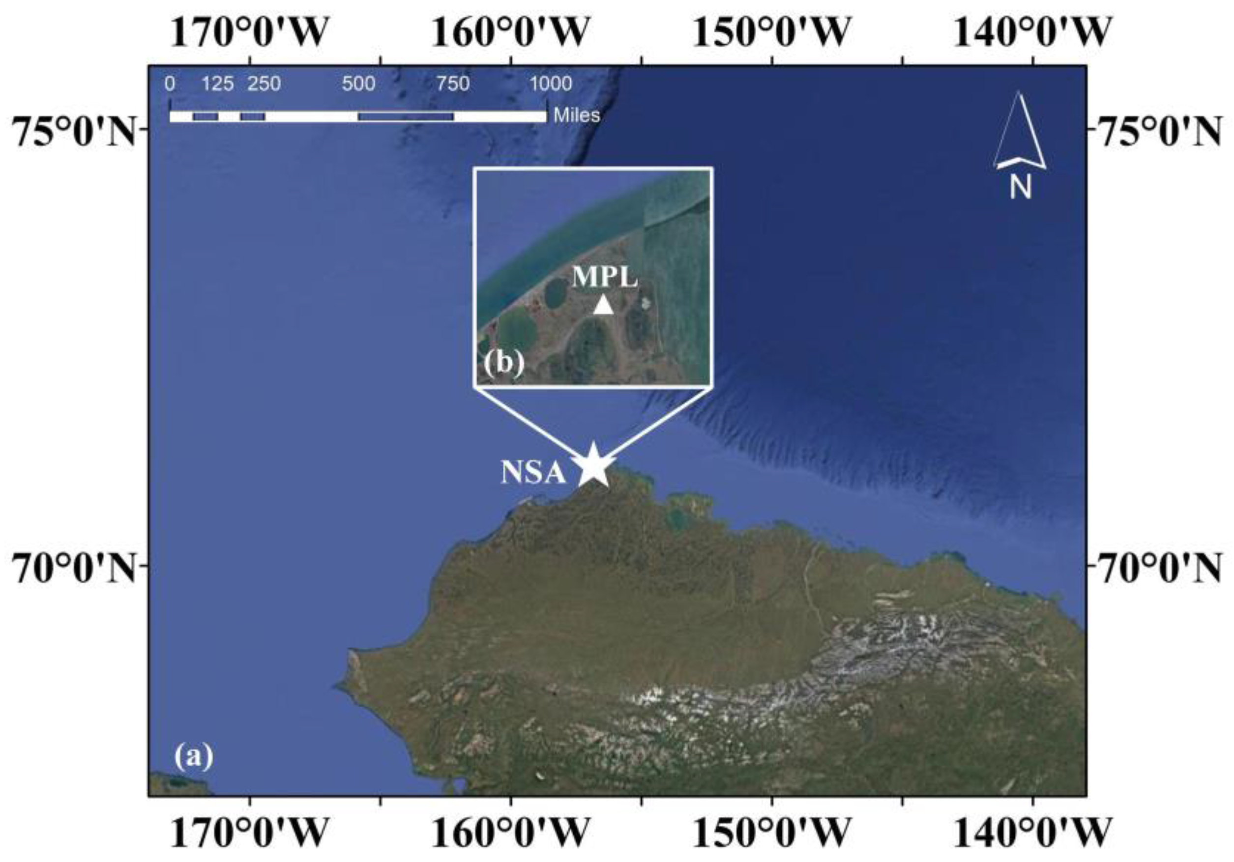
2.1. Study Area

The North Slope of Alaska (NSA) site, which is operated by the Atmospheric Radiation Measurement (ARM) User Facility, is anchored at Barrow, Alaska (71°19′N, 156°37′W), as illustrated in Figure 1. The NSA was established in 1997, and the facility serves as a critical Arctic observatory. This observatory is used to study climate amplification mechanisms, cryosphere–atmosphere interactions, and cloud-radiation processes under rapidly diminishing sea ice [30]. Situated on the Arctic coastal tundra, the Barrow facility benefits from proximity to the Chukchi Sea and Elson Lagoon, enabling observations of air masses transitioning between oceanic and continental regimes [31]. The NSA site hosts a comprehensive suite of instruments designed to address the unique challenges of Arctic climate research, including cloud radar, MPL, a microwave radiometer, etc. [32]. The NSA datasets have been instrumental in advancing understanding of mixed-phase cloud persistence, aerosol–cloud–radiation interactions, and Arctic amplification feedback. By integrating state-of-the-art remote sensing techniques, in situ measurements, and community-driven campaigns, the NSA site has become a foundational element in the domain of polar climate research, offering unparalleled insights into the rapidly transforming Arctic system [33].

2.2. Micropulse Lidar Data

The MPL is a ground-based optical remote sensing instrument primarily designed to determine cloud base height and monitor the vertical structure of atmospheric aerosols [34]. Operating at a wavelength of 532 nm, it emits short laser pulses and receives time-varying backscattered energy signals, enabling high-frequency dynamic observations of cloud and aerosol layers [35]. In this study, aerosol profile data obtained from the MPL, combined with range-corrected backscatter signals (RCS), were used to develop an algorithm for retrieving the PBLH [36]. The data processing involved the implementation of an hourly scale to suppress background noise interference. The effective detection height of the system’s signals begins at 150 m, with the raw observation data providing a temporal resolution of 10 s and a vertical resolution of 15 m. Detailed instrument performance parameters can be found in the technical literature [37,38]. The analysis utilized data from the sgpmplpolfsC1.b1 dataset, which encompasses the continuous observation period from July 2014 to March 2021.

2.3. Radiosonde Data

The radiosonde (RS), as an active atmospheric profiling device, provides high-precision vertical profile data for TEM, RH, WS, and atmospheric pressure (Pres) [39]. Routine soundings were conducted at least four times daily, based on Coordinated Universal Time (UTC) at 0500, 1100, 1700, and 2300 UTC, which correspond to local time (LT = UTC − 5) at 0000, 0600, 1200, and 1800 LT, respectively. Additional vertical soundings were performed at 0900, 1500, and 2100 LT during certain periods. The ARM PBL value-added data product (VAP) (nsapblhtsonde1mcfarlC1.c1) includes the estimated PBLH from RS data using three approaches: the Heffter method [40], the Richardson number method [41], and the Liu and Liang method [42]. In this study, the PBLH of the Richardson number method in the PBL VAP product was selected as the reference value. This study focuses on the analysis of vertical TEM profiles and turbulence intensity characteristics under both sea-breeze and non-sea-breeze conditions, using the radiosonde dataset (sgpsondeC1.a1) for 0600, 1200, 1500, and 2100 LT.

2.4. Other Data

The meteorological data utilized in this study, including TEM, RH, Pres, WS, and wind direction (WD), were obtained from the ARM Program’s Surface Meteorological Integrated Dataset (sgpmetE13.b1). Considering the topographical characteristics of the NSA, this study defines observational profiles with surface wind directions ranging from 0° to 90° (northeast to east) or 270° to 360° (west to north) as sea breeze events only if they persist for more than three hours. This wind direction range reflects typical onshore flow patterns driven by the coastal land–sea thermal differences. The study incorporated the ARM Optimal Estimation Dataset (sgparmbeatmC1.c1), which combines cloud microphysical properties, radiation transmission parameters, and surface thermodynamic observations to generate a multidimensional optimal estimate of atmospheric state variables [43]. Core parameters, such as sensible heat flux (SHF) and net radiation flux (netR), were specifically extracted from this dataset. The land and sea surface temperature data used in this study were obtained from the ERA5 monthly averaged data on single levels from 1940 to the present dataset. Specifically, monthly averaged 2 m surface temperature data is utilized. The data span from July 2014 to March 2021. After outlier removal, temporal alignment, and spatial consistency checks, a standardized hourly time series dataset was created. A total of 8176 valid observational profiles were obtained, of which 5292 profiles met the aforementioned sea breeze conditions, while the remaining 2884 profiles correspond to boundary layer thermodynamic structure observations under non-sea-breeze conditions.

3. Methodology

3.1. Retrieval Methods of PBLH

The traditional lidar gradient method (GM) estimates the PBLH based on the minimum local gradient of the RCS profile. The vertical gradient of the RCS profile was computed as the first derivative of the signal with respect to height:

$$G\left(z\right)={\displaystyle \frac{\mathrm{d}\left(RCS\right)}{\mathrm{d}\left(z\right)}}$$

(1)

where $z$ represents the vertical height. The PBLH is characterized by a sharp decrease in aerosol concentration, corresponding to a local extremum in the gradient profile [2,44,45]. In order to circumvent the potential impact of clouds on the PBLH inversion, cloud conditions were excluded using the cloud markers from the ceilometer data. However, this approach is susceptible to interference from multi-layer aerosol structures and background noise. In order to address these limitations, a random forest (RF) algorithm is employed in this study. It integrates lidar aerosol gradient profiles with meteorological conditions to reduce the impact of multi-layer aerosols in polar regions, thereby enhancing the accuracy of PBLH retrievals. RF is an ensemble learning method composed of multiple decision trees, with its core principle being the improvement of regression accuracy through averaging or weighting the predictions of individual trees [46]. In this study, the RF model uses the three minimum local gradients of the RCS signal (GM₁, GM₂, and GM₃), along with TEM, RH, WS, Pre, WD, SHF, and NetR as input features. The PBLH derived from the Richardson number method is used as the reference value, which demonstrates overall reliability under various PBL conditions. Zhang et al. [47] demonstrated that the Richardson number approach effectively balances physical mechanisms with observational adaptability, showing particular sensitivity in capturing shallow PBLH under stable conditions while avoiding systematic overestimations under convective or neutral regimes. Furthermore, the Richardson number-based PBLH is a standard product in the ARM VAP dataset, ensuring consistency and comparability across different studies. The RF model parameters are set to 300 decision trees and a minimum leaf node sample size of 5. Further details of the algorithm can be found in our previous study [36]. To validate the reliability of the model, a 10-fold cross-validation approach based on individual samples is applied. The results demonstrate that the RF-estimated PBLH exhibits a correlation coefficient of 0.76 with radiosonde-derived reference values, thereby indicating robust performance of the proposed model.

3.2. Theoretical Basis of Variable Importance in Projection Calculation

Variable importance in projection (VIP) is a crucial metric used to assess the contribution of predictor variables in a partial least squares regression (PLSR) model [48]. VIP values reflect the overall significance of each predictor variable within the regression model and are widely applied in feature selection and model optimization.

In the context of a PLSR model, the dependent variable Y is associated with the predictor variables X through a set of latent variables. The PLSR model extracts an optimal set of latent components to maximize the correlation between X and Y, thereby enhancing the predictive capability of the model [49]. The relative importance of each predictor variable within the PLSR model is evaluated by VIP values, facilitating the selection of the most representative features.

The calculation of VIP values is based on the contribution of each latent component to the variance explanation of Y, as well as the weight of each predictor variable in these latent components. The mathematical formulation is given by:

$$VI{P}_j=\sqrt{p\cdot {\sum }_{a=1}^A{\omega }_{ja}^2\cdot {\displaystyle \frac{SS{Y}_a}{SS{Y}_{total}}}}$$

(2)

where $p$ represents the total number of predictor variables, $A$ denotes the selected number of latent components, $w_{ja}$ is the weight of the $j$th variable in the $a$th latent component, $SS{Y}_a$ is the variance of $Y$ explained by the $a$th latent component, and $SS{Y}_{total}$ is the total variance of $Y$ [50]. Generally, when $VI{P}_j$ > 1, the corresponding variable is considered to have a significant contribution to the model and is usually retained, whereas variables with $VI{P}_j$ < 1 are deemed less important and may be considered for removal [51].

In this study, we select meteorological variables such as TEM, RH, WS, SHF, NetR, and Pres as predictor variables, with PBLH as the target variable. The PLSR method is employed to compute the VIP values of each meteorological factor, thereby exploring their contributions to the retrieval of PBLH. Since PBLH is influenced by multiple meteorological factors, PLSR mitigates the multicollinearity problem in the original dataset through dimensionality reduction and feature extraction while effectively identifying key influencing factors.

4. Results

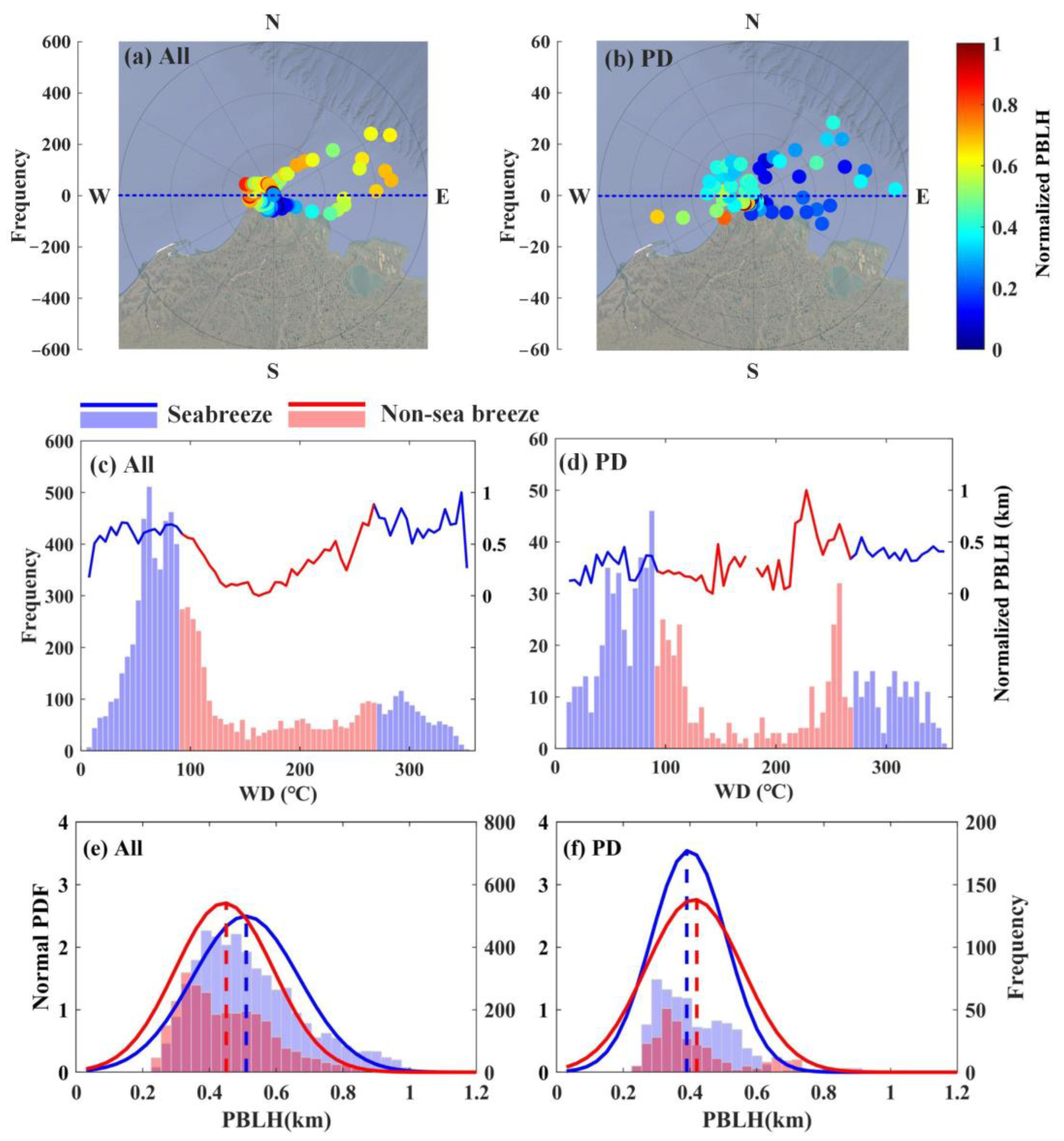
4.1. Statistical Analysis

Figure 2a,b present the frequency distributions of PBLH under different wind directions, with normalized PBLH values indicated by color. It is evident from both the annual (Figure 2a) and polar day (Figure 2b) conditions that PBLH varies significantly with wind direction, with the most pronounced changes occurring under the influence of sea breeze. On an annual scale, wind directions associated with sea breezes (primarily easterly and southeasterly winds) occur with relatively high frequency and correspond to generally elevated PBLH values, suggesting that sea breezes play a significant role in enhancing PBLH development. In contrast, non-sea-breeze directions are generally associated with lower PBLH. This phenomenon is likely related to changes in land–sea TEM differences and the duration of solar radiation exposure [52]. Since diurnal variations can have a large impact on the PBLH [53], in order to control the variables as much as possible, we selected periods of polar day and polar night to study the effect of the sea breeze on the evolution of the PBLH. However, since there are too few data during the polar night period, the subsequent study only analyzes the evolution of PBLH and the factors influencing it during the whole year and during the polar day period. During the polar day (Figure 2b), prolonged solar radiation leads to higher daytime TEM and more pronounced land–sea TEM contrast. Despite the continued dominance of sea breeze directions during the polar day, the associated PBLH values are notably lower, especially lower than those observed in the southwesterly direction under non-sea-breeze conditions. This suggests that during the polar day, the influence of the sea breeze leads to a more stable lower atmospheric structure, preventing the increase in PBLH. This could be due to the extended solar radiation during the polar day, which causes land TEM to be higher than those of the ocean, resulting in a stronger land–sea TEM contrast [54]. The cooler air brought by the sea breeze further enhances atmospheric stability, thereby limiting the vertical development of the PBLH [55]. Figure 2c,d further explore the joint distribution of wind direction and PBLH. Under annual conditions (Figure 2c), the frequency distribution exhibits prominent peaks at sea breeze directions (<90° and >270°), with the corresponding normalized PBLH curve (blue line) consistently higher than that associated with non-sea-breeze directions. In contrast, during the polar day (Figure 2d), although sea breeze directions remain dominant in frequency, their corresponding normalized PBLH values are generally lower than those under non-sea-breeze conditions. This indicates that during the polar day, stronger land–sea thermal inversion or the intrusion of cooler marine air may occur under sea breeze influence, leading to increased near-surface atmospheric stability and suppression of PBLH development.

Figure 2e,f present the probability density distribution of PBLH during sea breeze and non-sea-breeze periods. The blue line represents the sea breeze, while the red line represents the non-sea breeze. The blue and red histograms show the frequency of occurrence of PBLH during the respective periods. On the annual scale (Figure 2e), the PBLH distribution under sea breeze conditions is noticeably shifted to the right, with both its mean and peak values higher than those under non-sea-breeze conditions. The PBLH probability density during non-sea-breeze events peaks in the 0.4–0.5 km range, with a peak density of approximately 2.7. In contrast, the distribution during sea breeze periods shifts toward higher values, with a peak in the 0.5–0.6 km range, a slightly lower density (around 2.49). During the polar day period (Figure 2f), the peak of the PBLH probability density remains stable at around 0.4 km. In contrast, during non-sea-breeze periods, the probability density retains its single-peak structure, but the peak density decreases (approximately 0.75). The peak slightly shifts to 0.6 km. This phenomenon can be attributed to the cumulative effect of continuous solar radiation during the polar day, which increases surface energy [56]. Under non-sea-breeze conditions, prolonged daytime heating enhances sensible heat flux, promotes thermal convection, and significantly elevates PBLH. During sea breeze events, however, the interaction between cool, moist air advected from the ocean and land heating leads to stable stratification, restricting the boundary layer height to a lower range [57]. Moreover, the intensity and frequency of sea breeze circulation during the polar day may be higher, further reinforcing its suppressive effect on PBLH. The distribution characteristics of the histograms, showing a higher frequency of lower PBLH during sea breeze events, provide further evidence of this mechanism. It indicates that the sea breeze significantly regulates the diurnal evolution of the PBL structure through a coupling of thermal and dynamic processes. To further investigate the differences in land–sea TEM, the ERA5 surface TEM data were used to analyze the average land and sea surface TEM during both the annual period and the polar day.

As shown in Figure 3, clear differences exist in the TEM distributions between the ocean and land, with the land–sea TEM contrast being particularly pronounced during the polar day. During the annual period (Figure 3a), the TEM distribution appears relatively uniform, with ocean temperature being slightly higher than that of the land. The ocean TEM ranges from −8 °C to −7.5 °C, while the land TEM is significantly lower. This phenomenon suggests that, over the course of the year, the ocean, with its higher heat capacity and better thermal conductivity, results in relatively higher ocean TEM. In contrast, the land, with its lower heat capacity, experiences more significant TEM fluctuations, with higher daytime TEM and faster cooling at night. During the polar day (Figure 3b), the TEM distribution changes significantly. The ocean TEM is notably lower than that of the land, with ocean TEM ranging from 1 °C to 2 °C, showing a more uniform distribution. In comparison, land TEM values are clearly higher, ranging from 2 °C to 5 °C. This TEM difference indicates that, during the polar day, the extended duration of solar radiation allows the land to accumulate a substantial amount of heat, leading to higher TEM compared to the ocean. The ocean, however, experiences stronger radiative cooling, particularly during the polar day, causing its temperature to remain lower than that of the land [58]. This trend aligns with the variations observed in the PBLH during both the annual period and the polar day. Furthermore, during the polar day, the PBLH during sea breeze events is notably lower than at other times.

Figure 4 shows the diurnal variation of PBLH during sea breeze and non-sea-breeze periods. The blue line represents PBLH during sea breeze events, while the red line represents PBLH during non-sea-breeze periods. The blue and red stars correspond to RS-derived PBLH during sea breeze and non-sea-breeze periods, respectively. The background scatter points represent the density distribution of PBLH. From the annual diurnal variation (Figure 4a), it is evident that under sea breeze conditions, PBLH remains consistently higher than under non-sea-breeze conditions, with a relatively small diurnal range of approximately 0.5 km. This indicates a sustained influence of sea breezes in steadily promoting the development of the PBLH. In contrast, under non-sea-breeze conditions, the PBLH is generally lower (averaging around 0.43 km) and exhibits a slight afternoon increase, which may be associated with enhanced surface sensible heat flux and the triggering of localized convective activity. This discrepancy suggests that, on an annual average scale, sea breezes contribute to a persistent elevation of the PBLH by transporting warmer marine air inland (Figure 3a) and enhancing turbulence in the lower atmosphere, thereby maintaining a relatively high PBLH [59]. The consistency between RS-derived PBLH markers and lidar-based trends further supports the robustness of this conclusion. During the polar day period (Figure 4b), PBLH during sea breeze periods is lower than that during non-sea-breeze periods, and the overall variation remains small. In contrast, PBLH during non-sea-breeze periods shows more pronounced diurnal variation. During the day, PBLH rises rapidly and reaches its peak values in the morning and afternoon, ranging from 0.4 km to 0.5 km. This is likely due to the prolonged solar radiation during the polar day, which causes intense convective activity, thereby increasing the PBLH and reaching maximum PBLH values during the day. Additionally, during the polar day, the land–sea TEM contrast is more significant, primarily due to the cooling effect of the sea breeze, which enhances atmospheric stability and suppresses convective activity, keeping PBLH at lower levels [60]. To avoid the influence of diurnal variations on PBLH, subsequent research focuses solely on the impact of sea breeze on PBLH during the polar day period.

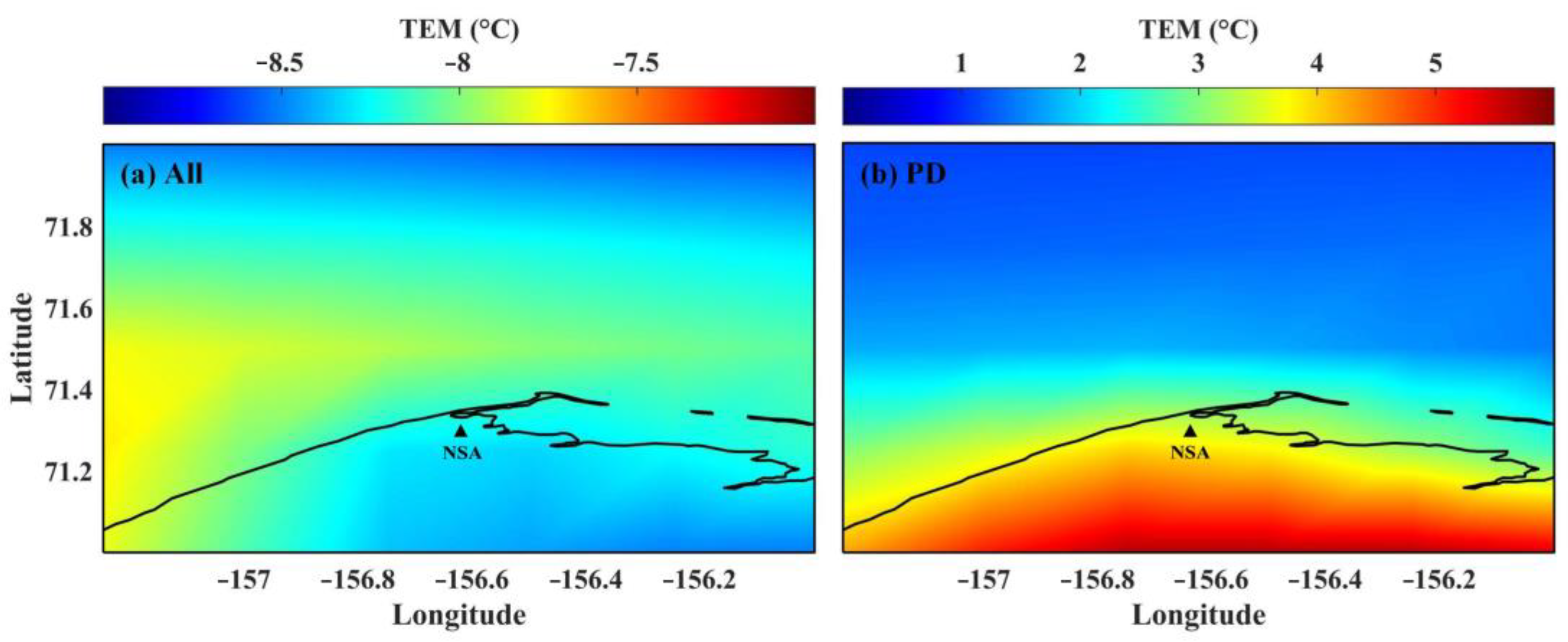
4.2. Meteorological Factors Under Sea Breeze and Non-Sea-Breeze Conditions

Figure 5 illustrates the vertical profiles of TEM (Figure 5a), WD (Figure 5b), and the square of the Brunt–Väisälä frequency (N², Figure 5c) under sea breeze and non-sea-breeze conditions during the polar day. In the TEM profile, the near-surface TEM during sea breeze conditions is lower than during non-sea-breeze conditions, with a smaller TEM gradient. The TEM change within the 0–0.3 km layer is within 2 °C, indicating a more uniform and stable vertical TEM distribution. In contrast, during non-sea-breeze periods, the near-surface TEM decreases sharply with height, reflecting the enhanced turbulent mixing driven by thermal instability. As demonstrated in Figure 5b, during periods of sea breeze, there is a marked enhancement in WS in the lower layer, with peak values exceeding 10 m/s. This is accompanied by strong vertical wind shear, indicating that horizontal momentum transfer driven by the sea breeze front dominates. In contrast, during non-sea-breeze periods, the vertical wind profile exhibits a more gradual slope, yet the standard deviation increases with height, suggesting active vertical momentum exchange due to turbulent mixing. It can be seen in Figure 5c that the differences in N² further highlight the characteristics of atmospheric stability. During sea breeze conditions, near-surface N² values are generally higher than on non-sea-breeze conditions (>0.5 × 10⁻³ s⁻²), indicating enhanced atmospheric stability under sea breeze conditions. This result is consistent with the TEM distribution, suggesting that the sea breeze reinforces low-level stability through the intrusion of cooler air. In contrast, near-surface N² values during non-sea-breeze periods tend to approach zero or become negative, indicating a potentially unstable stratification that is more favorable for convective development. The enhanced atmospheric stability suppresses vertical turbulent mixing, resulting in a lower PBLH during sea breeze conditions. This indirectly suggests that the sea breeze influences the development of PBLH by affecting atmospheric stability. This difference is attributed to the advection cooling effect of sea breeze circulation. When cool, moist air from the ocean intrudes over the land, it suppresses surface sensible heat flux and weakens the vertical temperature gradient, leading to a stable stratification [61]. Under non-sea-breeze conditions, prolonged solar radiation during the polar day heats the surface, driving intense thermal convection [62].

Figure 6 presents the diurnal variations of meteorological variables under sea breeze and non-sea-breeze conditions during the polar day. As demonstrated in Figure 6a, the diurnal variation of RH reveals that humidity is consistently higher during sea breeze periods compared to non-sea-breeze conditions, with the most significant differences occurring around noon. The histogram indicates that RH during non-sea-breeze periods is 10–15% lower than during sea breeze events. This difference is directly attributed to the advection of moist air from the ocean during the sea breeze conditions, while dry air masses dominate the land during non-sea-breeze periods, resulting in persistently lower humidity. The diurnal TEM variation shows the opposite trend. Surface TEM during non-sea-breeze periods peaks 3–5 °C higher than during sea breeze conditions, and the rate of TEM increase is faster. This is closely related to the absence of the sea breeze cooling effect and the efficient absorption of solar radiation by the dry land surface. The differences observed in NetR and SHF further support this mechanism. During sea breeze periods, NetR peaks are reduced by approximately 50 W/m², and SHF decreases by 30–40%, indicating that the advected oceanic air mass primarily weakens shortwave radiation absorption through increased cloud cover. Meanwhile, the colder land surface inhibits sensible heat transfer. Conversely, during non-sea-breeze periods, the absence of cooling from the sea breeze results in a significant increase in sensible heat flux, driving stronger turbulent mixing and PBLH uplift.

The diurnal variation of Pres and WS highlights the dynamic response of the land–sea circulation. During sea breeze periods, the afternoon Pres gradient significantly increases. The Pres is observed to be 1–2 hPa higher than during non-sea-breeze periods, accompanied by an earlier and stronger wind speed peak. The wind speeds exceed 6 m/s, which is 1–2 m/s higher than during non-sea-breeze periods, reflecting the acceleration of local circulation caused by the sea breeze. The histogram illustrates that, during sea breeze periods, Pres is typically higher, indicating that the sea breeze circulation may suppress the vertical development of the PBLH by enhancing atmospheric stability [63]. It is noteworthy that during the polar day, the extended daylight prolongs the development of the sea breeze, causing the meteorological differences in the afternoon to persist into the evening. For example, the sensible heat flux still shows a significant negative deviation at 20:00 LT. This thermal–dynamic coupling effect demonstrates that the sea breeze circulation not only reshapes the surface energy balance through advection cooling and moisture transport but also regulates boundary layer dynamics by altering the pressure gradient and vertical momentum distribution.

Figure 7 illustrates the distribution characteristics of meteorological parameters as a function of WS under sea breeze and non-sea-breeze conditions during the polar day. In the distribution of SHF (Figure 7a), the mean SHF for WS exceeding 3 m/s during sea breeze periods is significantly lower than during non-sea-breeze conditions, with the greatest difference observed at high WS (>9 m/s). This indicates that the advection cooling effect of the oceanic air mass stabilizes and suppresses surface sensible heat flux. In contrast, during non-sea-breeze periods, the dry air masses over land are continuously heated by prolonged polar day radiation, and the sensible heat flux increases with WS [64]. The TEM distribution further supports this mechanism. During sea breeze events, near-surface TEM values are generally lower than under non-sea-breeze conditions, with the maximum TEM difference reaching 5 °C. Additionally, TEM decreases slightly with increasing sea breeze WS. However, during non-sea-breeze periods, TEM rises significantly with increasing WS, reflecting the combined effects of land heating and turbulent mixing [65]. As shown in Figure 7c, both sea breeze and non-sea-breeze conditions exhibit a clear decrease in Pres with increasing WS, with Pres being higher during sea breeze periods than during non-sea-breeze periods. This could be due to enhanced vertical mixing with increasing WS, which lowers near-surface Pres in both conditions, while the higher overall Pres during sea breeze events may be influenced by oceanic high-pressure systems. In all WS ranges, NetR during sea breeze periods is consistently lower than during non-sea-breeze periods, suggesting that oceanic air masses reduce shortwave radiation absorption through increased cloud cover [66]. The RH distribution shows a clear separation, with high humidity (mean value > 88%) during sea breeze events and low humidity during non-sea-breeze periods. The largest difference in RH occurs at mid-to-high wind speeds, directly attributed to the transport of moist oceanic air and the suppression of local evaporation by dry land air masses. It is noteworthy that, with the exception of Pres, parameter differences between sea breeze and non-sea-breeze conditions converge at high WS (>9 m/s), indicating that under strong wind conditions, turbulent mixing dominates energy redistribution, weakening the local effects of land–sea thermal contrast. This phenomenon is consistent with the diurnal regulation of PBLH dynamic stability during the continuous daylight of the polar day. The cold, moist advection sea breeze enhances atmospheric stability, which in turn suppresses turbulent mixing, whereas thermal instability during non-sea-breeze conditions promotes turbulent mixing and enhances vertical energy transfer. Next, we investigated the impact of meteorological conditions on PBLH, as well as the specific mechanisms through which the sea breeze influences the PBLH.

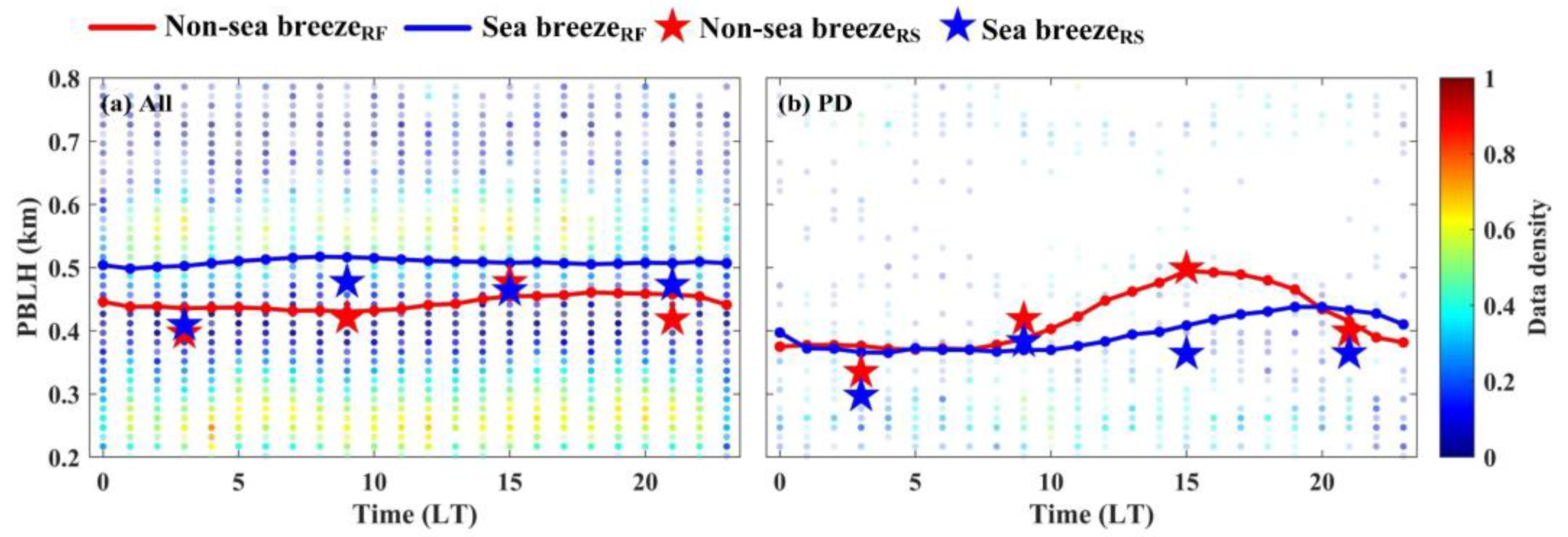
4.3. The Influence of Seabreeze on PBLH

Figure 8 presents the correlation coefficients between meteorological variables (Figure 8a) and the VIP contribution values of each meteorological parameter to PBLH (Figure 8b). From the correlation plots of various meteorological variables in Figure 8a, it is evident that TEM shows a positive correlation with RH, SHF, and NetR. The correlation analysis reveals a strong positive correlation between TEM and net NetR (R = 0.41), reflecting the direct effect of prolonged solar radiation heating the surface during the polar day. The positive correlation between TEM and SHF (R = 0.32) further supports the process of turbulent energy transfer from the surface to the atmosphere. Notably, the significant positive correlation between SHF and NetR (R = 0.52) suggests that increased NetR enhances the available surface energy, driving an increase in SHF, which in turn promotes the uplift of the PBLH [67]. Additionally, the weak negative correlation between TEM and WS (R = −0.16) implies that high WS may suppress surface warming by enhancing turbulent mixing or cold advection effects, thereby modulating the thermally driven development of the PBLH.

The VIP analysis further quantifies the differential impact of each variable on PBLH. The RH, with the highest VIP value (1.95), emerges as the primary controlling factor for PBLH. This mechanism can be attributed to the enhanced atmospheric stability under high humidity conditions. The advection of moist oceanic air reduces SHF (VIP value = 0.8) and increases latent heat distribution, thereby inhibiting the generation of turbulent kinetic energy and significantly limiting the uplift of PBLH [68]. Temperature (VIP = 1.1) follows in importance, affecting PBLH through dual pathways. On the one hand, surface heating (NetR VIP = 0.4) directly increases thermal instability, promoting convection. On the other hand, higher TEM may intensify the land–sea TEM contrast, indirectly strengthening the sea breeze’s suppressive effect on the PBLH [69]. Although the VIP values for SHF and NetR are lower (0.8 and 0.4, respectively), they still play an important role in influencing the diurnal variation of PBLH through energy redistribution and their synergistic effects with TEM and RH [70]. In contrast, WS (VIP = 0.41) and Pres (VIP = 0.1) contribute less, indicating that their effects are more dependent on the thermodynamic context, such as how high WS enhances atmospheric stability under sea breeze conditions or enhances vertical mixing under thermally unstable conditions during non-sea-breeze periods.

Finally, using the polar day period as an example, this study reveals the specific mechanisms through which the sea breeze influences the evolution of PBLH. As shown in Figure 9, during sea breeze events, the advection of cool, moist air from the ocean to the land leads to a decrease in near-surface TEM, while RH increases significantly, creating a stable atmospheric stratification. The TEM reduction directly weakens the SHF, along with potential increases in cloud cover, which results in reduced NetR, further limiting turbulent energy transfer from the surface to the atmosphere [71,72]. Although WS increases during sea breeze events, the accompanying strong vertical wind shear and cold advection jointly increase atmospheric stability, confining mechanical turbulence energy to the lower layers and preventing effective uplift of the PBLH. The comparison of TEM profiles further emphasizes the critical role of thermal stability. Prior to the sea breeze, higher TEM drives intense thermal convection, promoting the uplift of the PBLH. After the onset of the sea breeze, the TEM lapse rate near the surface (0–0.5 km) significantly decreases, forming an inversion or neutral stratification. Moreover, high RH increases air density and latent heat release, further reinforcing stratification stability [73]. This, in combination with low SHF, reduces the vertical transport efficiency of turbulent kinetic energy.

The continuous daylight during the polar day amplifies the land–sea thermal contrast, making the interaction between oceanic cold advection and land heating more pronounced, thereby further suppressing PBLH to lower heights during sea breeze events. This mechanism demonstrates that the sea breeze circulation systematically influences the development of PBLH through a combination of thermal control, involving TEM, RH, and stability, alongside dynamic control due to strong wind shear.

5. Conclusions

This study systematically investigates the regulatory role of sea breeze circulation on the PBLH in the Arctic coastal region, based on MPL, RS, and multi-source meteorological data collected from Barrow, Alaska, between July 2014 and March 2021. Statistical analysis reveals that sea breeze events significantly suppress PBLH development, with this effect being particularly prominent during the polar day. PBLH is notably lower during sea breeze events compared to non-sea-breeze conditions, with the peak of probability density distribution shifting toward lower PBLH ranges (0.4–0.6 km). During non-sea-breeze conditions, active land surface convection leads to a daily peak PBLH of up to 0.5 km. During sea breezes, the strong cold wind shear leads to a low-level inversion layer, which enhances atmospheric stability and leads to a significant decrease in PBLH. In contrast, under non-sea-breeze conditions, weak wind shear and TEM differences jointly drive PBLH uplift. Analysis of meteorological conditions shows that RH (VIP = 1.95) and TEM (VIP = 1.1) are the primary factors regulating PBLH variation. During sea breeze events, high RH suppresses turbulent development by reducing surface energy flux, while TEM differences intensify the land–sea thermal contrast, further strengthening the sea breeze circulation. The cold, moist air advection brought by the sea breeze reduces TEM and NetR, weakening available surface energy, thus limiting the development of the PBLH. During non-sea-breeze periods, land surface heating dominates, increasing SHF, and weak wind shear promotes thermal convection, driving daytime growth of PBLH.

In summary, the sea breeze regulates the Arctic PBL structure through a dual path of thermal and dynamical. The continuous solar radiation during the polar day further amplifies the land–sea TEM contrast, making the sea breeze effect a key driver in suppressing PBLH development. This study provides important observational evidence for PBL parameterization in polar climate models. However, the current conclusions are based on data from a single site, and future research should integrate multi-site observations and high-resolution simulations to explore the seasonal and interannual variations of the sea breeze mechanism and quantify its role in regulating Arctic aerosol transport and pollutant dispersion.

References

1. Seidel, D.J.; Ao, C.O.; Li, K. Estimating climatological planetary boundary layer heights from radiosonde observations: Comparison of methods and uncertainty analysis. J. Geophys. Res. Atmos. 2010, 115, D16. [Google Scholar] [CrossRef]
2. Stull, R.B. An Introduction to Boundary Layer Meteorology; Springer Science & Business Media: Berlin/Heidelberg, Germany, 1988; Volume 13. [Google Scholar]
3. LeMone, M.A. Boundary Layer (Atmospheric) and Air Pollution|Convective Boundary Layer. In Encyclopedia of Atmospheric Sciences, 2nd ed.; North, G.R., Pyle, J., Zhang, F., Eds.; Academic Press: Oxford, UK, 2015; pp. 250–257. [Google Scholar]
4. Seidel, D.J.; Zhang, Y.; Beljaars, A.; Golaz, J.C.; Jacobson, A.R.; Medeiros, B. Climatology of the planetary boundary layer over the continental United States and Europe. J. Geophys. Res. Atmos. 2012, 117, D17. [Google Scholar] [CrossRef]
5. Guo, J.; Miao, Y.; Zhang, Y.; Liu, H.; Li, Z.; Zhang, W.; He, J.; Lou, M.; Yan, Y.; Bian, L. The climatology of planetary boundary layer height in China derived from radiosonde and reanalysis data. Atmos. Chem. Phys. 2016, 16, 13309–13319. [Google Scholar] [CrossRef]
6. Holtslag, A.A.; Nieuwstadt, F.T. Scsaling the atmospheric boundary layer. Bound. Layer Meteorol. 1986, 36, 201–209. [Google Scholar] [CrossRef]
7. Garratt, J.R.; Hess, G.D. Boundary Layers|Neutrally Stratified Boundary Layer. In Encyclopedia of Atmospheric Sciences; Holton, J.R., Ed.; Academic Press: Oxford, UK, 2003; pp. 262–271. [Google Scholar] [CrossRef]
8. Xi, X.; Yang, Q.; Liu, C.; Shupe, M.D.; Han, B.; Peng, S.; Zhou, S.; Chen, D. Evaluation of the planetary boundary layer height from ERA5 reanalysis with MOSAiC observations over the Arctic Ocean. J. Geophys. Res. Atmos. 2024, 129, e2024JD040779. [Google Scholar] [CrossRef]
9. Peng, S.; Yang, Q.; Shupe, M.D.; Xi, X.; Han, B.; Chen, D.; Dahlke, S.; Liu, C. The characteristics of atmospheric boundary layer height over the Arctic Ocean during MOSAiC. Atmos. Chem. Phys. 2023, 23, 8683–8703. [Google Scholar] [CrossRef]
10. Heinemann, G. The polar regions: A natural laboratory for boundary layer meteorology—A review. Meteorol. Z. 2008, 17, 589. [Google Scholar] [CrossRef]
11. Dai, C.-Y.; Gao, Z.-Q.; Wang, Q.; Cheng, G. Analysis of atmospheric boundary layer height characteristics over the Arctic Ocean using the aircraft and GPS soundings. Atmos. Ocean. Sci. Lett. 2011, 4, 124–130. [Google Scholar]
12. Akansu, E.F.; Dahlke, S.; Siebert, H.; Wendisch, M. Evaluation of methods to determine the surface mixing layer height of the atmospheric boundary layer in the central Arctic during polar night and transition to polar day in cloudless and cloudy conditions. Atmos. Chem. Phys. 2023, 23, 15473–15489. [Google Scholar] [CrossRef]
13. Li, H.; Liu, B.; Gong, W.; Ma, Y.; Jin, S.; Wang, W.; Fan, R.; Jiang, S. Influence of clouds on planetary boundary layer height: A comparative study and factors analysis. Atmos. Res. 2025, 314, 107784. [Google Scholar] [CrossRef]
14. Anthes, R.A. The height of the planetary boundary layer and the production of circulation in a sea breeze model. J. Atmos. Sci. 1978, 35, 1231–1239. [Google Scholar] [CrossRef]
15. Miller, S.; Keim, B.; Talbot, R.; Mao, H. Sea breeze: Structure, forecasting, and impacts. Rev. Geophys. 2003, 41, 1011. [Google Scholar] [CrossRef]
16. De Tomasi, F.; Miglietta, M.M.; Perrone, M.R. The growth of the planetary boundary layer at a coastal site: A case study. Bound. Layer Meteorol. 2011, 139, 521–541. [Google Scholar] [CrossRef]
17. Abbs, D.J.; Physick, W.L. Sea-breeze observations and modelling—A review. Aust. Meteorol. Mag. 1992, 41, 7–19. [Google Scholar]
18. Challa, V.S.; Indracanti, J.; Rabarison, M.K.; Patrick, C.; Baham, J.M.; Young, J.; Hughes, R.; Hardy, M.G.; Swanier, S.J.; Yerramilli, A. A simulation study of mesoscale coastal circulations in Mississippi Gulf coast. Atmos. Res. 2009, 91, 9–25. [Google Scholar] [CrossRef]
19. Papanastasiou, D.; Melas, D. Climatology and impact on air quality of sea breeze in an urban coastal environment. Int. J. Climatol. J. R. Meteorol. Soc. 2009, 29, 305–315. [Google Scholar] [CrossRef]
20. Caicedo, V.; Rappenglueck, B.; Cuchiara, G.; Flynn, J.; Ferrare, R.; Scarino, A.; Berkoff, T.; Senff, C.; Langford, A.; Lefer, B. Bay breeze and sea breeze circulation impacts on the planetary boundary layer and air quality from an observed and modeled DISCOVER-AQ Texas case study. J. Geophys. Res. Atmos. 2019, 124, 7359–7378. [Google Scholar] [CrossRef]
21. Igel, A.L.; van den Heever, S.C.; Johnson, J.S. Meteorological and land surface properties impacting sea breeze extent and aerosol distribution in a dry environment. J. Geophys. Res. Atmos. 2018, 123, 22–37. [Google Scholar] [CrossRef]
22. He, J.; Kang, Y.; Wang, Y.; Gu, Y.; Zhong, K. Effects of sea-land breeze on air pollutant dispersion in street networks with different distances from coast using WRF-CFD coupling method. Sustain. Cities Soc. 2024, 115, 105757. [Google Scholar] [CrossRef]
23. Davis, S.R.; Farrar, J.T.; Weller, R.A.; Jiang, H.; Pratt, L.J. The land-sea breeze of the red sea: Observations, simulations, and relationships to regional moisture transport. J. Geophys. Res. Atmos. 2019, 124, 13803–13825. [Google Scholar] [CrossRef]
24. Aliabadi, A.; Staebler, R.; De Grandpré, J.; Zadra, A.; Vaillancourt, P. Comparison of estimated atmospheric boundary layer mixing height in the Arctic and southern Great Plains under statically stable conditions: Experimental and numerical aspects. Atmos. Ocean 2016, 54, 60–74. [Google Scholar] [CrossRef]
25. Davis, E.V.; Rajeev, K.; Mishra, M.K. Effect of clouds on the diurnal evolution of the atmospheric boundary-layer height over a tropical coastal station. Bound. Layer Meteorol. 2020, 175, 135–152. [Google Scholar] [CrossRef]
26. Liu, H.; Chan, J.C.; Cheng, A.Y. Internal boundary layer structure under sea-breeze conditions in Hong Kong. Atmos. Environ. 2001, 35, 683–692. [Google Scholar] [CrossRef]
27. Pal, S.; Clark, N.E.; Lee, T.R.; Conder, M.; Buban, M. When and where horizontal advection is critical to alter atmospheric boundary layer dynamics over land: The need for a conceptual framework. Atmos. Res. 2021, 264, 105825. [Google Scholar] [CrossRef]
28. Reddy, T.R.; Mehta, S.K.; Ananthavel, A.; Ali, S.; Annamalai, V.; Rao, D.N. Seasonal characteristics of sea breeze and thermal internal boundary layer over Indian east coast region. Meteorol. Atmos. Phys. 2021, 133, 217–232. [Google Scholar] [CrossRef]
29. Pal, S.; Lee, T.R. Contrasting air mass advection explains significant differences in boundary layer depth seasonal cycles under onshore versus offshore flows. Geophys. Res. Lett. 2019, 46, 2846–2853. [Google Scholar] [CrossRef]
30. Verlinde, J.; Zak, B.; Shupe, M.; Ivey, M.; Stamnes, K. The arm north slope of alaska (nsa) sites. Meteorol. Monogr. 2016, 57, 8.1–8.13. [Google Scholar] [CrossRef]
31. Spangenberg, D.; Chakrapani, V.; Doelling, D.; Minnis, P.; Arduini, R. Development of an automated Arctic cloud mask using clear-sky satellite observations taken over the SHEBA and ARM NSA sites. In Proceedings of the 6th Conference on Polar Meteorology and Oceanography, San Diego, CA, USA, 14–18 May 2001; pp. 14–18. [Google Scholar]
32. Qiu, S.; Dong, X.; Xi, B.; Li, J.L. Characterizing Arctic mixed-phase cloud structure and its relationship with humidity and temperature inversion using ARM NSA observations. J. Geophys. Res. Atmos. 2015, 120, 7737–7746. [Google Scholar] [CrossRef]
33. Doty, K.J. Metadata Systems for Arms SGP and NSA Sites; Brookhaven National Lab. (BNL): Upton, NY, USA, 1999. [Google Scholar]
34. Muradyan, P.; Coulter, R. Micropulse Lidar (MPL) Instrument Handbook. DOE/SC-ARM-TR-019, 20 pp. 2020. Available online: https://www.arm.gov/publications/tech_reports/handbooks/mpl_handbook.pdf (accessed on 4 May 2025).
35. Campbell, J.R.; Hlavka, D.L.; Welton, E.J.; Flynn, C.J.; Turner, D.D.; Spinhirne, J.D.; Scott III, V.S.; Hwang, I. Full-time, eye-safe cloud and aerosol lidar observation at atmospheric radiation measurement program sites: Instruments and data processing. J. Atmos. Ocean. Technol. 2002, 19, 431–442. [Google Scholar] [CrossRef]
36. Li, H.; Liu, B.; Ma, X.; Jin, S.; Wang, W.; Fan, R.; Ma, Y.; Wei, R.; Gong, W. Estimation of Planetary Boundary Layer Height from Lidar by Combining Gradient Method and Machine Learning Algorithms. IEEE Trans. Geosci. Remote Sens. 2023, 61, 1–11. [Google Scholar] [CrossRef]
37. Campbell, J.R.; Welton, E.J.; Spinhirne, J.D.; Ji, Q.; Tsay, S.C.; Piketh, S.J.; Barenbrug, M.; Holben, B.N. Micropulse lidar observations of tropospheric aerosols over northeastern South Africa during the ARREX and SAFARI 2000 dry season experiments. J. Geophys. Res. Atmos. 2003, 108, D13. [Google Scholar] [CrossRef]
38. Han, G.; Huang, Y.; Shi, T.; Zhang, H.; Li, S.; Zhang, H.; Chen, W.; Liu, J.; Gong, W. Quantifying CO2 emissions of power plants with Aerosols and Carbon Dioxide Lidar onboard DQ-1. Remote Sens. Environ. 2024, 313, 114368. [Google Scholar] [CrossRef]
39. Wang, W.; Li, B.; Chen, B. Improved surface NO2 Retrieval: Double-layer machine learning model construction and spatio-temporal characterization analysis in China (2018–2023). J. Environ. Manage. 2025, 384, 125439. [Google Scholar] [CrossRef]
40. Heffter, J. Transport layer depth calculations. Presented at the Second Joint Conference on Applications of Air Pollution Meteorology, New Orleans, LA, USA, 24–27 March 1980; American Meteorological Society: Boston, MA, USA, 1980; Volume 24, p. 28. [Google Scholar]
41. Richardson, H.; Basu, S.; Holtslag, A. Improving stable boundary-layer height estimation using a stability-dependent critical bulk Richardson number. Bound. Layer Meteorol. 2013, 148, 93–109. [Google Scholar] [CrossRef]
42. Liu, S.; Liang, X.-Z. Observed diurnal cycle climatology of planetary boundary layer height. J. Clim. 2010, 23, 5790–5809. [Google Scholar] [CrossRef]
43. Xie, S.; McCoy, R.B.; Klein, S.A.; Cederwall, R.T.; Wiscombe, W.J.; Clothiaux, E.E.; Gaustad, K.L.; Golaz, J.-C.; Hall, S.D.; Jensen, M.P. ARM climate modeling best estimate data: A new data product for climate studies. Bull. Am. Meteorol. Soc. 2010, 91, 13–21. [Google Scholar] [CrossRef]
44. Yang, J.; Gan, R.; Luo, B.; Wang, A.; Shi, S.; Du, L. An improved method for individual tree segmentation in complex urban scene based on using multispectral LiDAR by deep learning. IEEE J. Sel. Top. Appl. Earth Obs. Remote Sens. 2024, 17, 6561–6576. [Google Scholar] [CrossRef]
45. Li, H.; Chang, J.; Liu, Z.; Zhang, L.; Dai, T.; Chen, S. An improved method for automatic determination of the planetary boundary layer height based on lidar data. J. Quant. Spectrosc. Radiat. Transf. 2020, 257, 107382. [Google Scholar] [CrossRef]
46. Breiman, L. Random forests. Mach. Learn. 2001, 45, 5–32. [Google Scholar] [CrossRef]
47. Zhang, D.; Comstock, J.; Morris, V. Comparison of planetary boundary layer height from ceilometer with ARM radiosonde data. Atmos. Meas. Tech. 2022, 15, 4735–4749. [Google Scholar] [CrossRef]
48. Zheng, R.; Chen, Z.; Guan, Z.; Zhao, C.; Cui, H.; Shang, H. Variable importance for projection (VIP) scores for analyzing the contribution of risk factors in severe adverse events to Xiyanping injection. Chin. Med. 2023, 18, 15. [Google Scholar] [CrossRef] [PubMed]
49. Oussama, A.; Elabadi, F.; Platikanov, S.; Kzaiber, F.; Tauler, R. Detection of olive oil adulteration using FT-IR spectroscopy and PLS with variable importance of projection (VIP) scores. J. Am. Oil Chem. Soc. 2012, 89, 1807–1812. [Google Scholar] [CrossRef]
50. Farrés, M.; Platikanov, S.; Tsakovski, S.; Tauler, R. Comparison of the variable importance in projection (VIP) and of the selectivity ratio (SR) methods for variable selection and interpretation. J. Chemom. 2015, 29, 528–536. [Google Scholar] [CrossRef]
51. Mahieu, B.; Qannari, E.M.; Jaillais, B. Extension and significance testing of Variable Importance in Projection (VIP) indices in Partial Least Squares regression and Principal Components Analysis. Chemom. Intell. Lab. Syst. 2023, 242, 104986. [Google Scholar] [CrossRef]
52. Joshi, M.M.; Gregory, J.M.; Webb, M.J.; Sexton, D.M.; Johns, T.C. Mechanisms for the land/sea warming contrast exhibited by simulations of climate change. Clim. Dyn. 2008, 30, 455–465. [Google Scholar] [CrossRef]
53. Liu, B.; Ma, X.; Ma, Y.; Li, H.; Jin, S.; Fan, R.; Gong, W. The relationship between atmospheric boundary layer and temperature inversion layer and their aerosol capture capabilities. Atmos. Res. 2022, 271, 106121. [Google Scholar] [CrossRef]
54. Oksman, J. Proposed annual and sunspot cycle variation of the plasmasphere of the Earth. Nat. Phys. Sci. 1971, 231, 12–13. [Google Scholar] [CrossRef]
55. Faizal, M.; Rafiuddin Ahmed, M. On the ocean heat budget and ocean thermal energy conversion. Int. J. Energy Res. 2011, 35, 1119–1144. [Google Scholar] [CrossRef]
56. Gu, W.; Zhu, L.Y.; Cui, W.J.; Li, N.; Cong, J.O.; Xu, Y.J.; Huang, S.Q.; Yu, H.Y.; Li, L.T. The research of sea-land breeze (SLB) on the west coast of Bohai Bay based on field observation. Ences Cold Arid Reg. 2011, 3, 264–273. [Google Scholar]
57. Zhang, L.; Xin, J.; Yin, Y.; Wang, Z.; Wang, D.; Ma, Y.; Jia, D.; Jiang, Y.; Wu, L.; Pan, X. Adaptability evaluation of boundary layer schemes for simulation of sea and land breeze circulation in the west coast of the Yellow Sea. Atmos. Res. 2022, 278, 106354. [Google Scholar] [CrossRef]
58. Wild, M. Decadal changes in radiative fluxes at land and ocean surfaces and their relevance for global warming. Wiley Interdiscip. Rev. Clim. Change 2016, 7, 91–107. [Google Scholar] [CrossRef]
59. Cheung, T.K. Sodar observations of the stable lower atmospheric boundary layer at Barrow, Alaska. Bound. Layer Meteorol. 1991, 57, 251–274. [Google Scholar] [CrossRef]
60. Lee, Y.-H.; Park, M.-S.; Choi, Y. Planetary boundary-layer structure at an inland urban site under sea breeze penetration. Asia-Pac. J. Atmos. Sci. 2021, 57, 701–715. [Google Scholar] [CrossRef]
61. Liu, B.; Ma, Y.; Gong, W.; Zhang, M.; Yang, J. Determination of boundary layer top on the basis of the characteristics of atmospheric particles. Atmos. Environ. 2018, 178, 140–147. [Google Scholar] [CrossRef]
62. Rahman, K.; Rios, G.; Gamarro, H.; Addasi, O.; Peña, J.C.; Gonzalez-Cruz, J.; Bornstein, R.; Ramamurthy, P. The boundary layer characteristics of coastal urban environments. Theor. Appl. Climatol. 2024, 155, 6931–6948. [Google Scholar] [CrossRef]
63. Simpson, J.; Mansfield, D.; Milford, J. Inland penetration of sea-breeze fronts. Q. J. R. Meteorol. Soc. 1977, 103, 47–76. [Google Scholar]
64. Pithan, F.; Svensson, G.; Caballero, R.; Chechin, D.; Cronin, T.W.; Ekman, A.M.; Neggers, R.; Shupe, M.D.; Solomon, A.; Tjernström, M. Role of air-mass transformations in exchange between the Arctic and mid-latitudes. Nat. Geosci. 2018, 11, 805–812. [Google Scholar] [CrossRef]
65. Ju, T.; Wu, B.; Zhang, H.; Wang, Z.; Liu, J. Impacts of boundary-layer structure and turbulence on the variations of PM2.5 during fog–haze episodes. Bound. Layer Meteorol. 2022, 183, 469–493. [Google Scholar] [CrossRef]
66. Stapf, J.; Ehrlich, A.; Jäkel, E.; Lüpkes, C.; Wendisch, M. Reassessment of shortwave surface cloud radiative forcing in the Arctic: Consideration of surface-albedo–cloud interactions. Atmos. Chem. Phys. 2020, 20, 9895–9914. [Google Scholar] [CrossRef]
67. Xu, H.; Guo, J.; Li, J.; Liu, L.; Chen, T.; Guo, X.; Lyu, Y.; Wang, D.; Han, Y.; Chen, Q. The significant role of radiosonde-measured cloud-base height in the estimation of cloud radiative forcing. Adv. Atmos. Sci. 2021, 38, 1552–1565. [Google Scholar] [CrossRef]
68. Allabakash, S.; Lim, S. Climatology of planetary boundary layer height-controlling meteorological parameters over the Korean Peninsula. Remote Sens. 2020, 12, 2571. [Google Scholar] [CrossRef]
69. Darand, M.; Zandkarimi, F. Identification of atmospheric boundary layer height and trends over Iran using high-resolution ECMWF reanalysis dataset. Theor. Appl. Climatol. 2019, 137, 1457–1465. [Google Scholar] [CrossRef]
70. Miao, Y.; Guo, J.; Liu, S.; Liu, H.; Li, Z.; Zhang, W.; Zhai, P. Classification of summertime synoptic patterns in Beijing and their associations with boundary layer structure affecting aerosol pollution. Atmos. Chem. Phys. 2017, 17, 3097–3110. [Google Scholar] [CrossRef]
71. Mengis, N.; Martin, T.; Keller, D.P.; Oschlies, A. Assessing climate impacts and risks of ocean albedo modification in the Arctic. J. Geophys. Res. Ocean. 2016, 121, 3044–3057. [Google Scholar] [CrossRef]
72. Shupe, M.D.; Intrieri, J.M. Cloud radiative forcing of the Arctic surface: The influence of cloud properties, surface albedo, and solar zenith angle. J. Clim. 2004, 17, 616–628. [Google Scholar] [CrossRef]
73. Schneider, T.; O’Gorman, P.A.; Levine, X.J. Water vapor and the dynamics of climate changes. Rev. Geophys. 2010, 48, RG3001. [Google Scholar] [CrossRef]
Figure 1. The geographic location of (a) NSA site and (b) MPL equipment.
Remotesensing 17 01633 g001
Figure 2. Normalized PBLH and PBLH occurrence frequency for different wind directions under (a,c) annual period and (b,d) polar day conditions. The probability density distributions of PBLH during (e) annual period and (f) polar day conditions. The blue line represents the sea breeze, while the red line represents the non-sea breeze. The blue and red histograms show the frequency of occurrence of PBLH during the respective periods.
Remotesensing 17 01633 g002
Figure 3. Land and sea surface temperature for the (a) annual period and (b) polar day conditions.
Remotesensing 17 01633 g003
Figure 4. The diurnal variations of PBLH during (a) annual period and (b) polar day conditions.
Remotesensing 17 01633 g004
Figure 5. Vertical profiles of (a) temperature, (b) wind speed, and (c) square of Brunt–Väisälä frequency during polar day under sea breeze and non-sea-breeze conditions. The blue and red shading represent the standard deviation during sea breeze and non-sea-breeze periods, respectively.
Remotesensing 17 01633 g005
Figure 6. Daily variations of meteorological parameters: (a) RH, (b) TEM, (c) NetR, (d) SHF, (e) Pres, (f) WS. Non-sea-breeze (red) and sea breeze (blue) conditions are depicted with solid lines, accompanied by shaded bands showing the standard deviation. Vertical bars quantify diurnal contrasts between different conditions, with red bars marking enhanced values and blue bars reduced measurements.
Remotesensing 17 01633 g006
Figure 7. The variation of various meteorological conditions (a) SHF, (b) TEM, (c) Pres, (d) NetR, and (e) RH with WS during the polar day. The red and blue error bars represent the non-sea-breeze and sea breeze conditions, respectively. Gray dots represent the values for each type of meteorological condition.
Remotesensing 17 01633 g007
Figure 8. The (a) correlation coefficients between meteorological variables and (b) VIP contribution of meteorological variables to PBLH. The asterisks indicate that it passed the significance test (p < 0.05).
Remotesensing 17 01633 g008
Figure 9. Graphical representation of the specific mechanisms by the sea breeze on the PBLH. Red and blue arrows represent trends in meteorological factors. The red dashed curve and straight line represent the TEM profile and PBLH during the non-sea-breeze period, respectively. The blue solid curve and straight line represent the TEM profile and PBLH during the sea breeze period, respectively.
Remotesensing 17 01633 g009
Disclaimer/Publisher’s Note: The statements, opinions and data contained in all publications are solely those of the individual author(s) and contributor(s) and not of MDPI and/or the editor(s). MDPI and/or the editor(s) disclaim responsibility for any injury to people or property resulting from any ideas, methods, instructions or products referred to in the content.