A Shipborne Doppler Lidar Investigation of the Winter Marine Atmospheric Boundary Layer over Southeastern China’s Coastal Waters

Abstract

The Marine Atmospheric Boundary Layer (MABL), as a critical component of Earth’s climate system, governs the exchange of matter and energy between the ocean surface and the lower atmosphere. This study presents shipborne Doppler lidar observations conducted during 12 January to 3 February 2024, along the southeastern Chinese coast. Employing a Coherent Doppler Wind Lidar (CDWL) system onboard the R/V “Yuezhanyu” research vessel, we investigated the spatiotemporal variability of MABL characteristics through integration with ERA5 reanalysis data. The key findings reveal a significant positive correlation between MABL height and surface sensible heat flux in winter, underscoring the dominant role of sensible heat flux in boundary layer development. Through the Empirical Orthogonal Function (EOF) analysis of the ERA5 regional boundary layer height, sensible heat flux, and sea level pressure, we demonstrate MABL height over the coastal seas typically exceeds the corresponding terrestrial atmospheric boundary layer height and exhibits weak diurnal variation. The CDWL observations highlight complex wind field dynamics influenced by synoptic conditions and maritime zones. Compared to onshore regions, the MABL over offshore areas further away from land has lower wind shear changes and a more uniform wind field. Notably, the terrain of Taiwan, China, induces significant low-level jet formations within the MABL. Low-level jets and low boundary layer height promote the pollution episode observed by CDWL. This research provides new insights into MABL dynamics over East Asian marginal seas, with implications for improving boundary layer parameterization in regional climate models and advancing our understanding of coastal meteorological processes.

1. Introduction

The Marine Atmospheric Boundary Layer (MABL), as a critical component of the Earth’s climate system, plays an indispensable role in the exchange of energy, sensible heat, water vapor, and momentum between the ocean and the lower atmosphere [1,2]. The vertical structure of atmospheric elements is of significant importance for a deeper understanding of the driving and coupling mechanisms, as well as for the accurate parameterization of ocean–atmosphere interaction processes [3]. In weather forecasting, the precise detection of MABL characteristics and patterns can provide numerical models with accurate initial conditions and physical parameters, thereby enhancing the accuracy of both short-term and long-term predictions [4]. In offshore wind power development, a thorough analysis of the wind conditions within the MABL of specific maritime zones can ensure the efficient exploitation of offshore wind energy [5]. In the field of atmospheric pollution research, the formation of pollution events is often closely associated with atmospheric pollutant emissions and specific meteorological conditions [6,7,8]. Investigating the structure of the MABL contributes to the analysis of meteorological conditions, thereby providing scientific support for the prediction and prevention of pollution.

The Coherent Doppler Wind Lidar (CDWL) possesses the advantage of high spatiotemporal resolution, playing a significant role in MABL detection. CDWL is capable of accurately measuring key parameters within the MABL, such as wind field distribution, turbulence intensity, and boundary layer height (BLH), which are crucial for revealing the structural characteristics and dynamic properties of the MABL. When CDWL is utilized for MABL detection on a shipborne mobile platform, variations in the platform’s speed and attitude (roll, pitch, heading) can significantly impact the accurate acquisition of wind vectors. By employing correction algorithms to adjust the radial wind obtained from CDWL measurements, it is possible to derive the true atmospheric wind field within a geographic coordinate system [3,9]. Shipborne CDWL measurements offer wind profiles with high spatial and temporal resolution [10,11], enabling the determination of the turbulent structure within the MABL [12,13,14].

Despite the progress achieved in existing research, there remain certain limiting factors. Firstly, there is a scarcity of wintertime shipborne CDWL observation data, which may constrain our understanding of some complex phenomena within the MABL. Secondly, given the notable differences in MABL characteristics across various maritime regions, it is imperative to conduct long-distance shipborne observations to capture and compare regional MABL features.

This study utilized CDWL for wintertime shipborne observations of MABL along the southeastern coastal waters of China, aiming to elucidate the wind field structures and MABL characteristics under varying weather and maritime conditions. The shipborne experiment was conducted from 12 January to 3 February 2024, encompassing a round-trip cruise from Guangdong to Zhejiang and back to Guangdong. Furthermore, this study integrates ERA5 reanalysis data to further investigate the temporal and spatial variation patterns of the MABL.

2. Data and Methods

2.1. Shipborne Cruise Experiment

The northbound and southbound routes taken during the shipborne cruise experiment conducted from 12 January to 3 February 2024 are illustrated in Figure 1a. The CDWL was mounted on the second deck of the vessel for observation, as shown in Figure 1b,c. The specific routes of the round-trip cruise are as follows: (1) The northbound route commenced on 12 January and concluded on 20 January, departing from Zhanjiang, Guangdong, and sailing along the nearshore coastline to Zhoushan, Zhejiang; (2) From 21 January to 24 January, the research vessel docked at Zhoushan, Zhejiang, conducting continuous stationary observations under stable conditions; (3) The southbound route began on 25 January and ended on 3 February, setting sail from Zhoushan, Zhejiang, and following a zigzag course back to Zhanjiang, Guangdong.

2.2. Coherent Doppler Wind Lidar

The CDWL employed in this study was developed jointly by the Ocean University of China and Qingdao Leice Transient Technology Co., Ltd. (Qingdao, China). Wind field detection using Doppler lidar is based on the Doppler effect of light, which establishes a relationship between the Doppler shift and the radial wind speed along the laser beam direction. The atmospheric wind field is calculated using the CDWL by synthesizing radial wind speeds derived from non-coplanar measurements. Depending on the vertical distribution of aerosols, the CDWL can retrieve the BLH, allowing for high spatiotemporal resolution detection of the MABL height and wind field. The technical specifications of the CDWL in this experiment are as shown in

Table 1. Technical specifications of the CDWL in this experiment.

Parameters	Value
Laser wavelength	1550 nm
Pulse repetition frequency	10 kHz
Scan mode	Doppler beam swing mode (4 beams with an elevation angle of about 70° pointing to the east, south, west, and north of the device, as well as a vertical upward beam)
Single-beam accumulation time	1 s
Complete scanning cycle time	16 s

. Detailed equipment parameters and operating conditions can be found on the official website at https://www.leice-lidar.com/ (accessed on 22 April 2025).

During the cruise experiment, the CDWL employed a Doppler beam swing mode for wind and MABL detection, and the true atmospheric wind field was obtained through velocity and attitude correction [3]. The number of detection range gates was set to 300, with a vertical height range of 85 m to 8585 m and a vertical height resolution of approximately 28 m. The CDWL reached complete overlap above its minimum detection height of 85 m. The CDWL measured a raw wind profile every ~16 s. To reduce the bias of high-frequency measurements, the raw wind profile data were averaged over 10 min intervals. The gradient of the range-corrected SNR profile was used to retrieve the BLH [15], which provided MABL height measurements across varying weather and maritime conditions during the cruise. The resolution of the CDWL wind field, BLH, and other products used in this study are presented in

Table 2. Resolution of the CDWL products used.

Product	Temporal Resolution	Spatial Resolution
Wind speed	10 min average (averaged from originally measured profiles)	Detection altitude range: 85–8585 m; Vertical resolution: 28 m
Wind direction
SNR
Aerosol extinction coefficient
BLH
Cloud base height

.

2.3. ERA5 Reanalysis Dataset

ERA5 is a global atmospheric reanalysis model developed by the European Centre for Medium-Range Weather Forecasts. The hourly single-level reanalysis dataset [16] provided by ERA5 features a latitude–longitude grid resolution of 0.25° × 0.25° and encompasses hourly reanalysis data for atmospheric, ocean wave, and land surface variables.

Table 3. Resolution of the ERA5 reanalysis data used.

Product	Temporal Resolution	Spatial Resolution
BLH	1 h	Selected domain range: 105°E–125°E, 15°N–35°N; Grid resolution: 0.25° × 0.25°
Skin temperature (SKT)
Surface sensible heat flux (SHF)
Sea level pressure (SLP)

shows the resolution of the ERA5 reanalysis data used in this study.

2.4. Wind Shear Calculation

Wind shear reflects significant changes in the horizontal wind vector in the vertical direction and is calculated using the following formula:

$$S_{VW}={\displaystyle \frac{\sqrt{{(\Delta U)}^2+{(\Delta V)}^2}}{\Delta Z}}$$

(1)

Here, $S_{VW}$ is the vertical shear of the horizontal wind, $\Delta U$ is the change in the zonal component $U$ of the wind in the vertical direction, $\Delta V$ is the change in the meridional component $V$ of the wind in the vertical direction, and $\Delta Z$ represents the change in height in the vertical direction.

2.5. Empirical Orthogonal Function Analysis

The Empirical Orthogonal Function (EOF) analysis, initially proposed by Pearson [17], is a method for extracting characteristic quantities from matrix analysis. Lorenz [18] introduced this method into the field of atmospheric sciences for the extraction and study of the temporal and spatial variation characteristics of meteorological element fields.

In this study, the time series matrix $X$, composed of BLH, surface SHF, and SLP from the ERA5 reanalysis data, has a dimension of T × 3V. Here, T represents the temporal dimension, reflecting the length of the time series of the aforementioned three elements during the cruise period; V represents the spatial dimension, illustrating the spatial distribution of these three elements, covering the study area from 105°E to 125°E and 15°N to 35°N.

The time series matrix $X$, within the aforementioned study area during the cruise period, is as follows:

$$X=(H_{BL} F_{SH} P_{SL})$$

(2)

Here, $H_{BL}$ is the time series matrix of BLH, $F_{SH}$ is the time series matrix of surface SHF, and $P_{SL}$ is the time series matrix of SLP.

Specific decomposition steps are as follows:

Data Standardization: The BLH (unit: m), surface upward SHF (unit: W m⁻²), and SLP (unit: hPa) are standardized (mean = 0, variance = 1) to account for unit and magnitude differences. The standardization formula is as follows:

$$X_{std}={\displaystyle \frac{X-\mu }{\sigma }}$$

(3)

Here, $X$ is the time series matrix with a dimension of T × 3V; $\mu$ is the mean vector with a dimension of 1 × 3V, representing the mean of each variable; $\sigma$ is the standard deviation vector with a dimension of 1 × 3V, representing the standard deviation of each variable; and $X_{std}$ is the standardized data matrix with a dimension of T × 3V.

Calculate the Covariance Matrix: The covariance matrix $C$ for the standardized data matrix $X_{std}$ is computed. The formula for calculating the covariance matrix $C$ is as follows:

$$C={\displaystyle \frac{1}{T-1}}{X_{std}}^T{X}_{std}$$

(4)

Here, $C$ is the covariance matrix with a dimension of 3V × 3V; ${X_{std}}^T$ is the transpose of the standardized data matrix $X_{std}$ with a dimension of 3V × T.

Eigenvalue Decomposition: Eigenvalue decomposition is performed on the covariance matrix $C$ to find the eigenvalues ${\lambda }_i$ and the corresponding eigenvectors $e_i$. The eigenvalue decomposition of the covariance matrix $C$ is as follows:

$$C=E\Lambda E^T$$

(5)

Here, $E$ is the eigenvector matrix with a dimension of 3V × 3V, and its column vectors are the eigenvectors $e_i$; $\Lambda$ is a diagonal matrix with a dimension of 3V × 3V, and its diagonal elements are the eigenvalues ${\lambda }_i$; $E^T$ is the transpose of the eigenvector matrix $E$.

Calculate EOF: The EOF is the eigenvector matrix $E$ of the covariance matrix $C$, and its column vectors $e_i$ represent the $i$-th EOF mode.

Calculate Principal Components: The standardized data matrix $X_{std}$ is projected onto the EOF to obtain the principal component matrix $P$. The formula for calculating the principal component matrix $P$ is as follows:

$$P=X_{std}E$$

(6)

Here, $P$ is the principal component matrix with a dimension of T × 3V, and each column $p_i$ represents the principal component (PC) time series coefficients corresponding to the $i$-th EOF mode, with a dimension of T × 1.

Calculate the Variance of Each Mode: The variance of each mode is calculated using the eigenvalues ${\lambda }_i$. The variance $R_i$ of the $i$-th mode is calculated using the following formula:

$$R_i={\displaystyle \frac{{\lambda }_i}{{\displaystyle \sum {\lambda }_i}}}\times 100\%$$

(7)

Here, ${\lambda }_i$ is the $i$-th eigenvalue of the covariance matrix $C$, and the denominator ${\displaystyle \sum {\lambda }_i}$ is the sum of all eigenvalues.

After decomposition through the above steps, the EOF modes for BLH, surface SHF, and SLP fields are extracted in the order of the time series matrix $X$ composed of the three elements. These three fields share a common time series coefficient.

3. Results

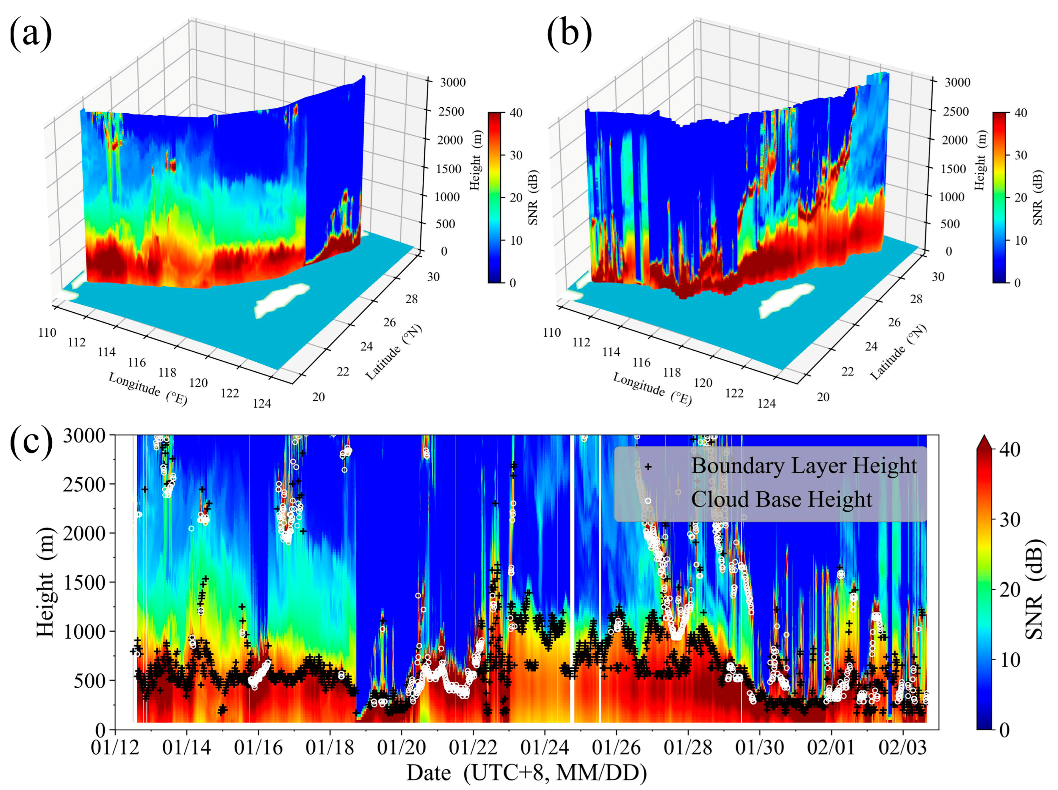
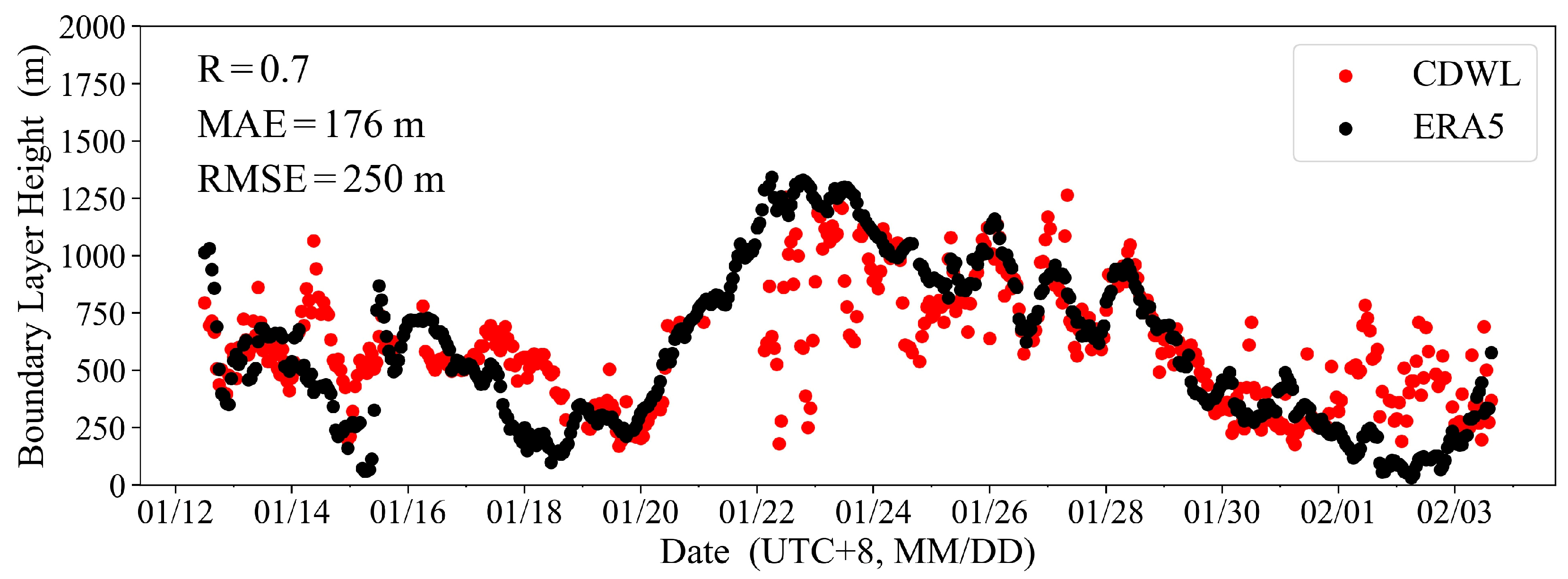
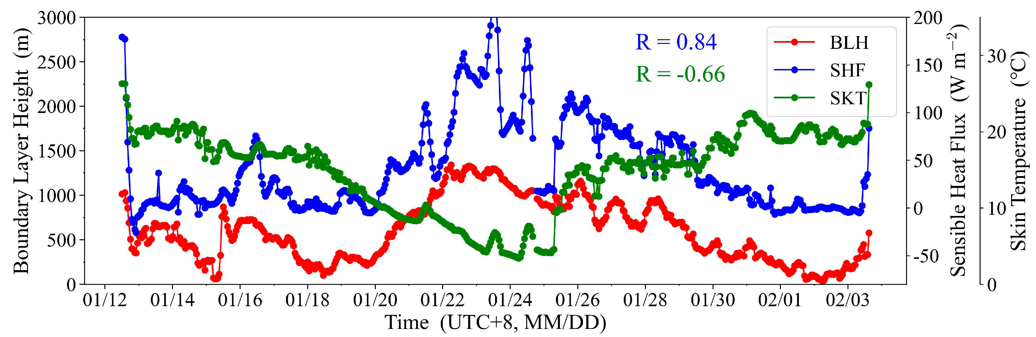
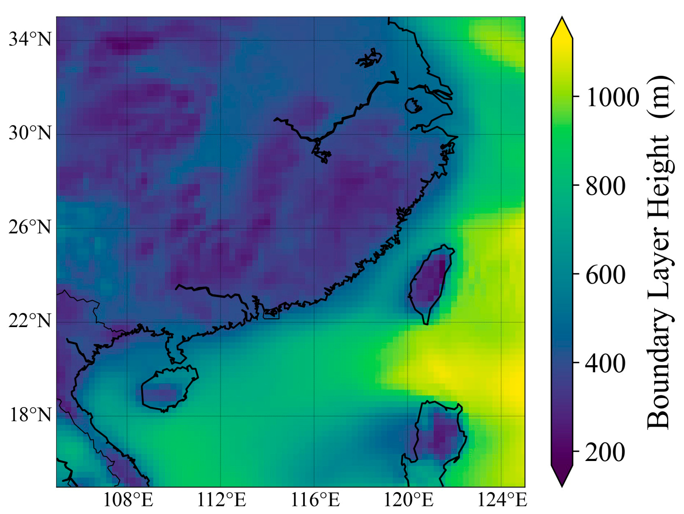
3.1. Characteristics of MABL Height

The SNR results of the CDWL during the cruise are shown in Figure 2, with the height display range set at 0–3000 m to highlight the boundary layer features. For shipborne Doppler lidar based on high-frequency detection, using the turbulent dissipation rate to determine the dynamic MABL height may result in low stability. In contrast, the distribution of substances within the boundary layer is relatively abundant, making the inversion of the MABL height using the SNR gradient method more stable. The BLHs retrieved using the gradient method [15] are annotated in Figure 2c. The retrieval results reveal complex spatiotemporal variation in the SNR, BLH, and cloud base height, reflecting the boundary layer characteristics of different maritime areas under various weather conditions.

During the nights of 26 January and 27 January on the southbound cruise, the CDWL reached maritime areas far from the coastline, where relatively high BLHs were recorded. That is, the MABL height was greater when away from the coast and land. This is different from those boundary layer development characteristics observed during the northbound cruise (13 January to 15 January, and 17 January) and docking at Zhoushan, Zhejiang (22 January to 24 January), near the land within the harbor, where the BLH is higher during the day and lower at night [19]. In addition, the CDWL captured low clouds during cold and warm air mass convergence (19 January to 22 January, and 29 January to 31 January) and sea fog under low-pressure system dominance (1 February to 3 February).

Based on the BLH development characteristics captured by the CDWL in different regions, further analysis was conducted in conjunction with ERA5 reanalysis data. Firstly, using the actual BLH results from the CDWL as a benchmark, the accuracy of the ERA5 reanalysis data during the cruise period was evaluated. The 10 min average BLH of CDWL was averaged into hourly results and compared with ERA5 data at the hourly navigation location grid point. The BLHs at the grid points where the CDWL was located during the cruise were extracted, and the hourly average BLHs from the CDWL were compared with those from ERA5 (Figure 3). The BLHs of the ERA5 reanalysis results were consistent with the trends detected by the CDWL, with a correlation coefficient R of 0.7. This result indicates that the ERA5 reanalysis data have a certain reliability in describing variations in BLH. However, the mean absolute error (MAE) was 176 m and the root-mean-square error (RMSE) was 250 m. The reason for this discrepancy lies in the fact that the CDWL retrieves the material BLH using the SNR gradient method, while ERA5 retrieves the dynamic BLH using the Richardson number threshold method. There are inherent differences between the two methods. Additionally, the CDWL was influenced by the height distribution of aerosol particles within the boundary layer (such as from 26 January to 28 January), as well as sea fog and low clouds (such as from 19 January to 22 January, and 29 January to 3 February), which leads to significant changes in the BLH results retrieved by the CDWL. During these periods, the ERA5 BLHs do not fully align with the CDWL observations. Even though these differences exist, the BLH data provided by ERA5 can still be used to analyze the characteristics of BLH due to its extensive coverage and high temporal resolution.

A quantitative analysis of the correlation between the BLH, the surface upward SHF, and SKT from ERA5 reanalysis data during the cruise period was conducted. The results are shown in Figure 4. The BLH was negatively correlated with SKT, with a correlation coefficient of −0.66 (p < 0.001). However, BLH showed a strong positive correlation with SHF, with a correlation coefficient of 0.84 (p < 0.001). This significant positive correlation indicates that SHF has an important influence on the variation of BLH. In regions with higher SHF, more heat is transported into the atmosphere, promoting the upward development of the boundary layer, and BLH tends to be higher. This reveals the crucial role of SHF in driving boundary layer development.

The regional distribution of the mean BLH from ERA5 during the overall cruise period is shown in Figure 5. In southeastern China, the winter MABL height is generally higher than that over land, indicating spatial differences in BLH [20,21].

To further analyze the characteristics of BLH and its land–sea differences, we used the EOF method to decompose the time series matrix composed of BLH, SHF, and mean SLP in the southeastern region of China. The data used in this study are from ERA5 reanalysis data products covering the study area (longitude range 105°E to 125°E, latitude range 15°N to 35°N) during the cruise period for BLH, SHF, and SLP. Figure 6 shows that the first five EOF modes of BLH, SHF, and SLP explain 80% of the total variance, with EOF1 (41%) and EOF2 (22%) being the dominant modes.

In this study, we focused on analyzing EOF1 and EOF2 (Figure 7 and Figure 8), the two primary modes during the winter. As shown in Figure 7, EOF1 reveals that there are spatial differences in the EOF amplitudes of BLH, with strong positive amplitudes over the near-shore marine areas and weak positive and negative amplitudes over land. The SHF over the near-shore marine regions is relatively consistent with BLH. The coastal areas display strong positive amplitudes for SLP, indicating that strong weather systems primarily affect the coastal regions, where the variations in SLP are more pronounced. The Time coefficient PC shows positive high values during the period of 21 January to 29 January, corresponding to the weather process of strong cold air transit. During this period, the SLP in the coastal areas significantly increased under the influence of strong cold air. Due to the high heat capacity of the ocean, the sea surface temperature is less affected by strong cold air, and the SHF in near-shore coastal areas is higher, favoring the development of BLH. However, the low heat capacity of land means that the land surface temperature is more susceptible to weather system influences and decreases, which results in smaller SHF, weaker land–air heat exchange, and lower BLH. Meanwhile, the subsidence motion may inhibit the development of the boundary layer.

Under the influence of strong weather systems during the winter (overall cruise period), the different properties of the ocean and land surfaces lead to different responses to the transit of strong cold air. This reflects the small changes in BLH over land and large changes over the sea. When strong cold air transits, the land with low heat capacity responds quickly to the weather system. The surface temperature decreases quickly and the SHF changes little, resulting in small changes in BLH. For the sea, with high heat capacity, the response to the weather system is stable, the surface temperature is stable, and the SHF changes significantly, leading to large changes in BLH.

Figure 8 shows that the EOF2 amplitudes of BLH are positive in most regions, with higher amplitudes over land and lower amplitudes over the sea. This indicates that within the study area of this mode, the BLH generally exhibits a consistent trend of variation. However, the BLH changes more rapidly over land than over sea, while the changes over the sea are not significant. The SHF shows a trend consistent with the BLH, suggesting that when SHF increases more rapidly, BLH also rises faster. Conversely, when SHF decreases more rapidly, BLH also falls faster. This mode reflects a weak weather system background, as indicated by the SLP. Under the background of a weak weather system, the Time coefficient PC shows positive high values from 11:00 to 16:00 daily (UTC + 8). This suggests that the atmospheric boundary layer over land develops faster in the afternoon with higher BLHs, under the influence of solar radiation. In contrast, the changes in marine atmospheric BLH are relatively slower. During other periods, negative PC values suggest a faster decrease in land atmospheric BLH, while marine atmospheric BLH maintains relatively stable values.

Under the background of weak weather systems during winter, the different properties of the sea and land surfaces lead to different responses to solar radiation, reflecting the large diurnal variation of BLH over land and the lack of large diurnal variation over the sea. For land, low heat capacity results in high SHF during the day due to daytime heating effects and low SHF at other times. This leads to a significant diurnal variation in atmospheric BLH over land, being higher during the day and lower at night. The high heat capacity of the sea results in small diurnal variations in SHF, and the diurnal variation in MABL height is not significant.

EOF decomposition of regional BLH, SHF, and SLP demonstrates contrasting marine and terrestrial boundary layer development during strong weather systems (EOF1) and weak-condition backgrounds (EOF2). EOF1 reflects that under the influence of strong weather systems, land coastal area responds quickly to weather systems with small changes in SHF and BLH, whereas the sea responds slowly to weather systems with large changes in SHF and BLH. EOF2 reflects the impact of diurnal variations in solar radiation on SHF and BLH under weak weather system conditions. The daytime heating effect leads to high SHF over land during the day and low SHF at other times, with BLH exhibiting a diurnal variation characteristic of being higher during the day and lower at night. For the ocean, the high heat capacity results in small diurnal variations in SHF and no significant diurnal variation in BLH. Combined with the EOF results, the winter BLH reveals two key features: (1) marine values are consistently higher than over land, and (2) diurnal variation is weak.

3.2. Wind Field Characteristics

The wind speed and direction detected by the CDWL during the southbound cruise are shown in Figure 9. The wind speed and direction were influenced by different weather conditions and various maritime zones, which exhibit distinct stratification characteristics and complex spatiotemporal variation patterns. During this period, at high altitudes, wind direction was dominated by northwest and westerly, while at low altitudes, wind direction transitioned from northwest and northeast to southeast. Affected by high and low altitude weather systems, a low wind speed zone and a wind direction transition zone formed at 1–2 km altitude.

Influenced by the terrain of Taiwan, China, the northeastern airflow reaching the Taiwan Strait is accelerated by the blocking and guiding effects of the terrain. This significantly increases the wind speed within the boundary layer and results in northeast low-level jets with jet speeds exceeding 15 m s⁻¹. The terrain of Taiwan, China, favors the formation of boundary-layer low-level jets through topographic obstruction [22], though no such jets were observed during the northbound cruise due to interactions with low-level weather systems.

Figure 10a shows the CDWL wind shear detection during the overall cruise period, with the BLH superimposed. The CDWL observed strong wind shear at the top of the boundary layer, consistent with the characteristics observed by Wulfmeyer and Janjić [2] using shipborne Doppler lidar. The daily wind shear within the BLH detected by the CDWL is shown in the box plot in Figure 10b. As can be seen from Figure 10b, the wind shear within the MABL is lower in maritime areas far from land (26 January to 27 January), which differs from the higher wind shear characteristics within the MABL when the cruise is close to land. The differences in wind shear characteristics indicate that there are intense spatiotemporal variations in the wind field in near-shore marine areas [12]. Compared to areas close to land, the wind field within the MABL far from land is more uniform. The primary cause is that land has higher surface roughness than the sea.

From the wind field structure detected by the CDWL, it is evident that different maritime areas are influenced by varying weather conditions, resulting in stratified characteristics of wind speed and direction. The terrain of Taiwan, China, facilitates the formation of low-level jets within the boundary layer, while the wind field within the MABL is more uniform in areas far from land.

3.3. Pollution Episode

The aerosol extinction coefficient serves as a reliable proxy for particulate matter (e.g., PM_2.5) concentrations [23]. CDWL could also retrieve the aerosol extinction coefficient based on several assumptions, such as lidar ratio, boundary value, or reference height. It should be emphasized that the CDWL-retrieved aerosol optical properties must be calibrated by the collocated reference instruments, such as Raman lidars [24], high-spectral resolution lidar, or sun photometer [24,25]. The iteration algorithms, calibrated with collocated sun photometer, were incorporated into the CDWL employed in this study to derive the aerosol extinction coefficient [25]. During the southbound cruise, CDWL detected a significant pollution episode (from 01/25 to 01/29. Subsequently, this pollution episode was removed by wet precipitation), with vertical profiles of extinction coefficients shown in Figure 11. The vertical distribution characteristics of the extinction coefficients indicate that pollutants are confined within the MABL.

This pollution episode occurred under the influence of strong cold air transit. The orographic effect of Taiwan, China, enhanced the northeast low-level jets within the MABL (with speeds exceeding 15 m s⁻¹; Figure 9), which substantially intensified the horizontal transport of pollutants. Concurrently, the MABL height gradually decreased from 1000 m to 500 m, resulting in a 50% reduction in vertical ventilation volume, which enhanced pollutant accumulation. The concurrence of low-level jets and low BLH conditions promoted this pollution episode.

4. Discussion

The MABL exhibits a strong positive correlation with surface SHF in this investigation, underscoring the dominant role of SHF in boundary layer development. Nevertheless, the boundary layer dynamics are also influenced by other factors (e.g., aerosols and clouds). Their underlying mechanisms require further study.

During the Taiwan Strait transect, the CDWL observed low-level jets within the MABL with speeds exceeding 15 m s⁻¹. This phenomenon is likely attributed to the acceleration of northeasterly airflow by the blocking and channeling effects of Taiwan’s terrain. Compared to nearshore regions, the wind field within the MABL over open ocean areas exhibits greater uniformity. The enhanced wind shear observed near land may result from rougher underlying surfaces, which could facilitate pollutant mixing within the boundary layer. Notably, the combined effects of low-level jets, strong wind shear, and shallow boundary layers may intensify pollution episodes. In the future, more cases are needed to study the impact of meteorological factors on pollution episodes.

Due to the scarcity of marine atmospheric observations compared to terrestrial data, numerical models often exhibit larger biases over oceanic regions. Shipborne Doppler lidar measurements of the MABL could provide critical validation datasets, offering the potential to improve model parameterizations.

5. Conclusions

This study conducted a shipborne cruise experiment utilizing the CDWL jointly developed by the Ocean University of China and Qingdao Leice Transient Technology Co., Ltd., to investigate the MABL along the southeastern coast of China from 12 January to 3 February 2024. In conjunction with the ERA5 reanalysis dataset, this study provided an in-depth analysis of the MABL height and wind field characteristics.

The comparison of the CDWL and ERA5 reanalysis data indicates a high consistency in describing the variations of MABL height, with a correlation coefficient of 0.7. Despite certain discrepancies, the ERA5 reanalysis data still hold significant value in the study of BLH characteristics. The winter MABL height is generally higher than that over land. A significant positive correlation exists between the BLH and the surface SHF (R = 0.84, p < 0.001), suggesting that SHF plays a crucial role in driving boundary layer development. EOF decomposition of the ERA5 regional BLH during the overall cruise period reveals two main modes: EOF1 and EOF2. These two main modes reflect the development characteristics of the marine and terrestrial BLHs in winter. The winter MABL height is high with weak diurnal variation, and it is generally higher than that over land.

The wind field detection using Doppler lidar reveals complex spatiotemporal features under different weather conditions and maritime zones. The terrain of Taiwan, China, significantly affects the formation of low-level jets within the boundary layer. Compared to that in areas close land, the wind shear within the MABL is lower and the wind field is more uniform in areas far from land. The CDWL captured low clouds and sea fog induced by synoptic weather systems. Meanwhile, the CDWL observed wind direction transitions from northwest/northeast to southeast at low altitudes.

The CDWL extinction coefficients captured a pollution episode confined within the MABL. The concurrence of low-level jets and low BLH conditions promoted this pollution episode.

The findings of this study are of great significance for understanding the dynamic processes of the MABL and analyzing the meteorological conditions of pollution processes. Future research could further explore the detailed mechanisms behind BLH variations under different maritime and weather conditions.

References

1. Rogers, D.P.; Johnson, D.W.; Friehe, C.A. The stable internal boundary layer over a coastal sea. Part I: Airborne measurements of the mean and turbulence structure. J. Atmos. Sci. 1995, 52, 667–683. [Google Scholar] [CrossRef]
2. Wulfmeyer, V.; Janjić, T. Twenty-four-hour observations of the marine boundary layer using shipborne NOAA high-resolution Doppler lidar. J. Appl. Meteorol. 2005, 44, 1723–1744. [Google Scholar] [CrossRef]
3. Zhai, X.; Wu, S.; Liu, B.; Song, X.; Yin, J. Shipborne wind measurement and motion-induced error correction of a coherent Doppler lidar over the Yellow Sea in 2014. Atmos. Meas. Tech. 2018, 11, 1313–1331. [Google Scholar] [CrossRef]
4. Rubio, H.; Kühn, M.; Gottschall, J. Evaluation of low-level jets in the southern Baltic Sea: A comparison between ship-based lidar observational data and numerical models. Wind. Energy Sci. 2022, 7, 2433–2455. [Google Scholar] [CrossRef]
5. Shu, Z.R.; Li, Q.S.; He, Y.C.; Chan, P.W. Observations of offshore wind characteristics by Doppler-LiDAR for wind energy applications. Appl. Energy 2016, 169, 150–163. [Google Scholar] [CrossRef]
6. Wang, T.; Jiang, F.; Deng, J.; Shen, Y.; Fu, Q.; Wang, Q.; Fu, Y.; Xu, J.; Zhang, D. Urban air quality and regional haze weather forecast for Yangtze River Delta region. Atmos. Environ. 2012, 58, 70–83. [Google Scholar] [CrossRef]
7. Yang, Y.; Zheng, X.; Gao, Z.; Wang, H.; Wang, T.; Li, Y.; Lau, G.N.; Yim, S.H. Long-term trends of persistent synoptic circulation events in planetary boundary layer and their relationships with haze pollution in winter half year over eastern China. J. Geophys. Res.-Atmos. 2018, 123, 10–991. [Google Scholar] [CrossRef]
8. Zheng, Z.; Li, Y.; Wang, H.; Ding, H.; Li, Y.; Gao, Z.; Yang, Y. Re-evaluating the variation in trend of haze days in the urban areas of Beijing during a recent 36-year period. Atmos. Sci. Lett. 2018, 20, e878. [Google Scholar] [CrossRef]
9. Zentek, R.; Kohnemann, S.H.; Heinemann, G. Analysis of the performance of a ship-borne scanning wind lidar in the Arctic and Antarctic. Atmos. Meas. Tech. 2018, 11, 5781–5795. [Google Scholar] [CrossRef]
10. Tucker, S.C.; Senff, C.J.; Weickmann, A.M.; Brewer, W.A.; Banta, R.M.; Sandberg, S.P.; Hardesty, R.M. Doppler lidar estimation of mixing height using turbulence, shear, and aerosol profiles. J. Atmos. Ocean. Tech. 2009, 26, 673–688. [Google Scholar] [CrossRef]
11. Achtert, P.; Brooks, I.M.; Brooks, B.J.; Moat, B.I.; Prytherch, J.; Persson, P.O.G.; Tjernström, M. Measurement of wind profiles by motion-stabilised ship-borne Doppler lidar. Atmos. Meas. Tech. 2015, 8, 4993–5007. [Google Scholar] [CrossRef]
12. Pichugina, Y.L.; Banta, R.M.; Brewer, W.A.; Sandberg, S.P.; Hardesty, R.M. Doppler lidar-based wind-profile measurement system for offshore wind-energy and other marine boundary layer applications. J. Appl. Meteorol. Clim. 2012, 51, 327–349. [Google Scholar] [CrossRef]
13. Kumer, V.M.; Reuder, J.; Dorninger, M.; Zauner, R.; Grubišić, V. Turbulent kinetic energy estimates from profiling wind LiDAR measurements and their potential for wind energy applications. Renew. Energy 2016, 99, 898–910. [Google Scholar] [CrossRef]
14. Wang, X.; Dai, G.; Wu, S.; Zhu, P.; Li, Z.; Song, X.; Zhang, S.; Xu, J.; Yin, J.; Qin, S.; et al. Classification of turbulent mixing driven sources in marine atmospheric boundary layer with use of shipborne coherent doppler lidar observations. J. Geophys. Res.-Atmos. 2023, 128, e2023JD038918. [Google Scholar] [CrossRef]
15. Flamant, C.; Pelon, J.; Flamant, P.H.; Durand, P. Lidar determination of the entrainment zone thickness at the top of the unstable marine atmospheric boundary layer. Bound.-Lay. Meteorol. 1997, 83, 247–284. [Google Scholar] [CrossRef]
16. Hersbach, H.; Bell, B.; Berrisford, P.; Biavati, G.; Horányi, A.; Muñoz Sabater, J.; Nicolas, J.; Peubey, C.; Radu, R.; Rozum, I.; et al. ERA5 Hourly Data on Single Levels from 1940 to Present [Dataset]. Copernicus Climate Change Service (C3S) Climate Data Store (CDS). 2023. Available online: https://cds.climate.copernicus.eu/datasets/reanalysis-era5-single-levels?tab=overview (accessed on 22 April 2025).
17. Pearson, K. On lines and planes of closest fit to systems of point in space. Philos. Mag. 1901, 2, 559–572. [Google Scholar] [CrossRef]
18. Lorenz, E.N. Empirical Orthogonal Functions and Statistical Weather Prediction; Sci. Rep. 1; Massachusetts Institute of Technology, Department of Meteorology: Cambridge, MA, USA, 1956. [Google Scholar]
19. Stull, R.B. An Introduction to Boundary Layer Meteorology; Springer: Berlin/Heidelberg, Germany, 1988. [Google Scholar]
20. Banta, R.M.; Senff, C.J.; White, A.B.; Trainer, M.; McNider, R.T.; Valente, R.J.; Fehsenfeld, F.C. Daytime buildup and nighttime transport of urban ozone in the boundary layer during a stagnation episode. J. Geophys. Res.-Atmos. 1998, 103, 22519–22544. [Google Scholar] [CrossRef]
21. Banta, R.M.; White, A.B. Mixing-height differences between land use types: Dependence on wind speed. J. Geophys. Res.-Atmos. 2003, 108, 4321. [Google Scholar] [CrossRef]
22. Du, Y.; Chen, Y.; Zhang, Q. Numerical simulations of the boundary layer jet off the southeastern coast of China. Mon. Weather Rev. 2015, 143, 1212–1231. [Google Scholar] [CrossRef]
23. Cui, L.; Song, X.; Yang, Y.; Liu, J.; Li, Z.; Yun, L.; Zhang, M. Doppler lidar retrieval of particulate matter concentration based on statistical regression method. Acta Photon. Sin. 2021, 50, 1201005. [Google Scholar] [CrossRef]
24. Chouza, F.; Reitebuch, O.; Groß, S.; Rahm, S.; Freudenthaler, V.; Toledano, C.; Weinzierl, B. Retrieval of aerosol backscatter and extinction from airborne coherent Doppler wind lidar measurements. Atmos. Meas. Tech. 2015, 8, 2909–2926. [Google Scholar] [CrossRef]
25. Dai, G.; Wang, X.; Sun, K.; Wu, S.; Song, X.; Li, R.; Yin, J.; Wang, X. Calibration and retrieval of aerosol optical properties measured with Coherent Doppler Lidar. J. Atmos. Ocean. Technol. 2021, 38, 1035–1045. [Google Scholar] [CrossRef]
Figure 1. Configuration of the shipborne cruise experiment. (a) Northbound and southbound routes; (b) Location of the Doppler wind lidar; (c) Exterior view of the Doppler wind lidar.
Remotesensing 17 02161 g001
Figure 2. SNR detected by CDWL. (a) SNR during the northbound cruise; (b) SNR during the southbound cruise; (c) SNR, BLH, and cloud base height during the overall cruise. (Light blue on the map background indicates seawater areas, and white indicates land areas).
Remotesensing 17 02161 g002
Figure 3. Comparison of BLH between CDWL and ERA5.
Remotesensing 17 02161 g003
Figure 4. ERA5 BLH, surface SHF, and SKT.
Remotesensing 17 02161 g004
Figure 5. Mean BLH from ERA5 during the overall cruise period.
Remotesensing 17 02161 g005
Figure 6. Explained variance by EOF modes.
Remotesensing 17 02161 g006
Figure 7. EOF1. Standardized EOF amplitude (a) BLH; (b) SHF; (c) SLP; (d) Time coefficient PC.
Remotesensing 17 02161 g007
Figure 8. EOF2. Standardized EOF amplitude (a) BLH; (b) SHF; (c) SLP; (d) Time coefficient PC.
Remotesensing 17 02161 g008
Figure 9. (a) Wind speed and (b) direction detected by CDWL. (The light blue map background indicates seawater areas, and white indicates land areas).
Remotesensing 17 02161 g009
Figure 10. Wind shear detected by CDWL. (a) Wind shear; (b) Wind shear within the boundary layer. (The middle line of the box represents the median value of daily wind shear within the boundary layer, the box represents the interquartile range of wind shear within the boundary layer, the upper and lower edges of the box whiskers represent the normal distribution range of wind shear within the boundary layer, data points outside the upper and lower edges represent daily wind shear outliers within the boundary layer, and the color of the box represents the magnitude of the mean wind shear within the boundary layer, with cool colors indicating smaller means and warm colors indicating larger means).
Remotesensing 17 02161 g010
Figure 11. Aerosol extinction coefficient, BLH, and cloud base height detected by CDWL during the pollution episode.
Remotesensing 17 02161 g011