The Study on Landslide Hazards Based on Multi-Source Data and GMLCM Approach

Abstract

The southwest region of China is characterized by numerous rugged mountains and valleys, which create favorable conditions for landslide disasters. The landslide-influencing factors show different sensitivities regionally, which induces the occurrence of disasters to different degrees, especially in small sample areas. This study constructs a framework for the identification, analysis, and evaluation of landslide hazards in complex mountainous regions within small sample areas. This study utilizes small baseline subset interferometric synthetic aperture radar (SBAS-InSAR) technology and high-resolution optical imagery for a comprehensive interpretation to identify landslide hazards. A geodetector is employed to analyze disaster-inducing factors, and machine-learning models such as random forest (RF), gradient boosting decision tree (GBDT), categorical boosting (CatBoost), logistic regression (LR), and stacking ensemble strategies (Stacking) are applied for landslide sensitivity evaluation. GMLCM stands for geodetector–machine-learning-coupled modeling. The results indicate the following: (1) 172 landslide hazards were identified, primarily concentrated along the banks of the Lancang River. (2) A geodetector analysis shows that the key disaster-inducing factors for landslides include a digital elevation model (DEM) (1321–1857 m), rainfall (1181–1290 mm/a), the distance from roads (0–1285 m), and geological rock formation (soft rock formation). (3) Based on the application of the K-means clustering algorithm and the Bayesian optimization algorithm, the GD-CatBoost model shows excellent performance. High-sensitivity zones were predominantly concentrated along the Lancang River, accounting for 24.2% in the study area. The method for identifying landslide hazards and small-sample sensitivity evaluation can provide guidance and insights for landslide monitoring and harnessing in similar geological environments.

1. Introduction

Landslides are widely distributed all over the world and are one of the natural disasters with strong destructive power [1]. Climate change and the intensification of human activities will lead to an increase in the frequency of landslides, posing a serious threat to infrastructure and the lives of people and hindering social development [2]. Identifying, analyzing, and evaluating the sensitivity of early landslides in complex mountainous areas can provide local governments with a foundational framework for managing landslide risk zones and guide land-use planning [3,4].

Traditional landslide identification and cataloguing primarily rely on field surveys, which pose significant challenges in vast and topographically complex regions [5]. Since the 1970s, researchers have employed a combination of remote-sensing imagery and ground survey data for the manual visual interpretation of landslides [6]. However, optical remote-sensing technology has certain limitations in landslide identification. The quality of optical imagery is easily affected by weather conditions, particularly in areas with cloud cover, and it is challenging to effectively detect landslides that involve minor deformations. Subsequently, various remote-sensing data sources have emerged, including radar, SAR, InSAR, satellite stereo imagery, high-resolution images, drone imagery, and light detection and ranging (LiDAR) [7,8,9]. InSAR is a microwave remote-sensing technology that has developed rapidly in recent years. Compared to the traditional way, it has the advantage of superior wide coverage, high resolution, all-day detection, and high monitoring accuracy. All of these make up for the insufficiency of the traditional methods of recognizing and monitoring landslides in the mountainous areas, especially in places difficult to be reached by ground-monitoring means [10]. Currently, the mainstream methods for landslide identification based on InSAR technology include differential InSAR (D-InSAR), permanent-scatterer InSAR (PS-InSAR), and SBAS-InSAR [11,12,13]. Among them, SBAS-InSAR can effectively alleviate the problems of incoherence and atmospheric effect caused by a too-long spatial baseline in D-InSAR. At the same time, SBAS-InSAR improves the temporal sampling frequency, so that it can more accurately obtain the deformation information of slopes and reveal their safety state [14]. Compared with PS-InSAR, the deformation maps obtained by SBAS-InSAR are more continuous in spatial resolution, giving it a significant advantage in the monitoring of landslides in mountainous areas [15]. In recent years, many scholars have used SBAS-InSAR to carry out landslide-monitoring research, carried out with the aim of realizing the early identification and determination of landslides. These researchers have achieved remarkable results [16,17]. Although InSAR is widely used in landslide research, challenges remain in mountainous areas. Dense vegetation and steep terrain can cause data incoherence, while geometric distortions and atmospheric disturbances complicate the analysis. Relying on data from a single orbit may also lead to misidentifying landslides. These issues emphasize the need for more comprehensive monitoring methods, such as high-resolution imagery and multi-orbit approaches, to improve landslide detection accuracy.

Landslide sensitivity evaluation is used to assess the probability of landslides occurring. The effectiveness of landslide sensitivity modeling depends not only on the quality of the algorithms used but also on the screening of disaster triggers, the handling of positive and negative landslide samples, and the treatment of missing values, noise, and erroneous data [18]. Currently, the selection of landslide disaster-inducing factors relies mainly upon expert experience, but a uniform indicator system may not be fully applicable in different geo-geological contexts [19]. With the advantages of the geodetector in identifying spatial differentiation and understanding of the mechanisms of influencing factors, this method has gradually been applied for use in geological disaster factor identification and has achieved significant results [20]. In landslide sensitivity modeling, common machine-learning methods include LR, support vector machines (SVM), RF, GBDT, and CatBoost [21]. Deep-learning models, such as Transformer, long short-term memory networks (LSTM), and convolutional neural networks (CNN), are also gradually being applied in this field [22]. Using the example of Piedmont in Italy, Taalab demonstrated that RF can generate highly accurate landslide susceptibility maps for large heterogeneous areas without multiple evaluations [23]. Gu introduces a semi-supervised learning method for the screening of non-landslide samples, and the results show that the method works best when combined with CatBoost [24]. Akgun concluded that LR was the most accurate model based on the evaluation of its results using the area under the curve (AUC) [25]. In addition to single classifiers, many scholars have used stacking and deep-learning models to manage complex data and accurately predict landslide-sensitive areas [26,27,28]. Although there are many kinds of landslide sensitivity evaluation models, the practical application effect will still be affected by many factors. Hence, it remains essential to establish a corresponding model demonstration study for the areas with specific geological characteristics.

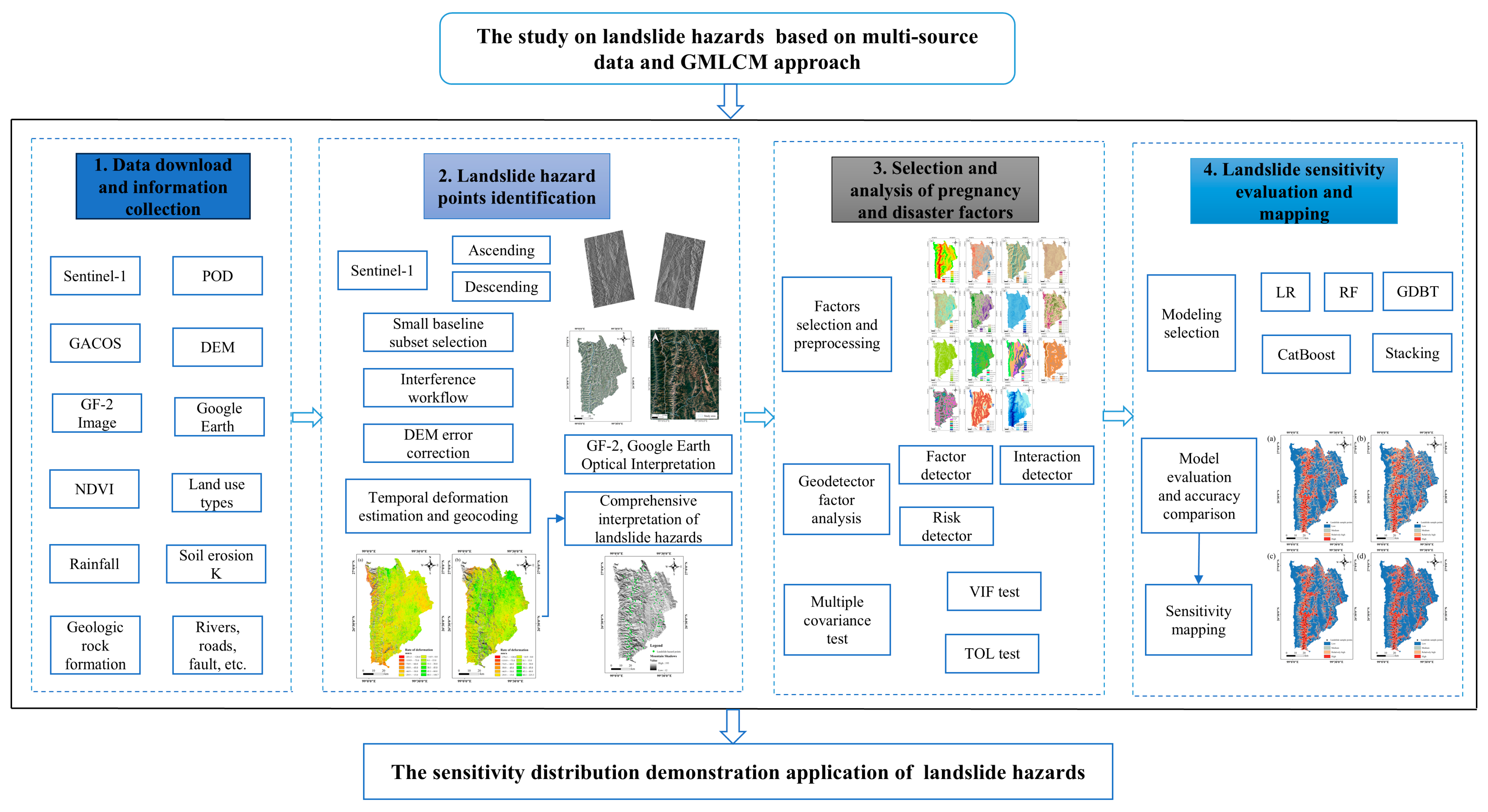
The purpose of this paper is to explore an integrated method that is applicable to the identification, analysis, and sensitivity evaluation of landslide hazards in small samples in complex mountainous areas. Taking Lamping County as the study area, this study combines two-track data, applies SBAS-InSAR technology with high-resolution optical imagery for landslide hazard interpretation, and analyzes disaster-inducing factors through the geodetector. The GD–machine-learning model is further constructed to carry out a demonstration study of landslide sensitivity evaluation for small samples, which provides guidance and reference for landslide research in similar geo-geographical environments.

2. Study Area and Data Sources

2.1. Study Area

Lanping is situated in the northwest of Yunnan Province, China, between 26°06′N and 27°04′N latitude (Figure 1). It is located in the deep canyon area of the Hengduan Mountains of China, in the belly of the “Three Rivers” area, where some of the landslide hazards are nurtured.

Lanping is characterized by high mountains and deep valleys, influenced by a combination of plateau and mountainous geographical conditions, and belongs to the subtropical plateau monsoon climate. There are 93 rivers, 14 of which are major rivers, all belonging to the Lancang River basin, covering a runoff area of 3573.8 km². The precipitation primarily occurs in the form of rainfall, with a concentration in July and August. The average annual precipitation is 1163 mm, and the total annual precipitation for the entire county is approximately 5.022 billion m³. The slope of the study area is predominantly between 20° and 30°, with high-slope areas primarily distributed along the western section of the Lancang River basin, and low-slope areas located in the southeastern part near Tongdian Town. The study area spans across two secondary structural units: the Lanping–Simao block of the Three Rivers Arc–Basin system and the Lancang River Junction Zone.

The geological and geographical conditions in Lanping are complex, and there are also significant spatial and temporal climate variations that make it one of the counties most affected by landslide disasters.

2.2. Data Sources

Sentinel-1 is an important part of the European Space Agency’s Copernicus program (ESA). Due to the side-viewing geometry of SAR satellites, there are differences in the geometric distortion and sensitivity to the surface deformation between the ascending and descending SAR images. This study uses C-band data to conduct landslide hazard identification (

Table 1. Sentinel-1 data information.

Orbit Path	Ascending	Ascending	Descending
Azimuth/(°)	−13.16	−13.16	−166.93
Angle of incidence/(°)	39.48	39.48	33.75
Distance and azimuthal resolution/m	2.33 × 13.97	2.33 × 13.97	2.33 × 13.97
Multiview spatial resolution/m	15	15	15
Time span	1 January 2023–31 October 2024	1 January 2023–31 October 2024	1 January 2023–26 October 2024
Path	99	99	33
Frame	1270	1265	502
Number	46	46	45
Polarization pattern	VV	VV	VV

).

The study data are as shown in

Table 2. Data used in the study.

Data Types	Data Sources	Formats
Sentinel-1 SAR	ESA	Zip
ALOS DEM	ASF	Tiff
POD	ESA	Eof
GACOS	GACOS website (www.gacos.net)	Tiff
GF-2 hyperspectral imagery	Yunnan Remote Sensing Center	Tiff
NDVI	Google Earth Engine	Tiff
Land use data	Esri	Shp
Rainfall data	National Tibetan Plateau Data Center	Tiff
Soil erosion factor K	Earth Resources Data Cloud Platform (www.gis5g.com)	Tiff
Roads, administrative boundaries, etc.	Open Platform for Digital Earth	Shp
Drone photos, geological and geographic data, and landslide historical ledger points	Project “2024 Yunnan Provincial Key Areas Geological Disaster Fine Investigation and Risk Evaluation (Lanping County)”	Shp

. To remove the terrain phase, calculate the geometric distortion areas, and perform geocoding of the results. A 12.5 m spatial resolution DEM, produced by the Japan Aerospace Exploration Agency and sourced from the Alaska Satellite Facility (ASF), was employed. The collected DEMs were resampled to extract inversion products such as the elevation, slope, aspect, curvature, surface roughness, terrain undulation, and topographic wetness index (TWI). These products, along with land-use data, soil erosion K-factor, rainfall, engineering geological formations, roads, faults, and river data, were used for a landslide hazards factor analysis and a sensitivity evaluation.

3. Methods

The route map of this study is shown in Figure 2. Taking Lanping County as the study area, Sentinel-1 ascending and descending data from January 2023 to October 2024 were processed using SBAS-InSAR to obtain the surface deformation rate. Landslide hazards were then interpreted comprehensively using the deformation rate, GF-2 imagery, and Google Earth. Based on the geological conditions and the previous research, relevant indicator factors were selected, and the geodetector was applied to analyze the landslide hazard factors. Additionally, multiple machine-learning models were used for landslide sensitivity evaluation and comparative analysis.

3.1. Landslide Hazard Identification Approach

SBAS-InSAR

SBAS-InSAR improves the absolute accuracy of the results, the capability to manage discontinuous or nonlinear time series, and the spatial coverage. By utilizing short temporal baselines and large spatial baselines between the SAR images, SBAS-InSAR overcomes decorrelation in both time and space, enabling a more reliable monitoring of the results with fewer data. The main steps are as follows:

The first step is to obtain a series of X + 1 images with the same characteristics taken at specific times (t₀, t₁, … t_n), where X is assumed to be an odd number. These images can be used to estimate the number of differential interferograms (M) for the low coherence signal component, as follows:

$${\displaystyle \frac{\mathrm{X}+1}{2}}\le \mathrm{M}\le \mathrm{X}\left({\displaystyle \frac{\mathrm{X}+1}{2}}\right)$$

(1)

where X represents the number of images and M represents the number of differential interferograms used to estimate the low-pass signal components.

The interferometric phase is expressed as follows:

$$\Delta {\phi }_{\theta }(\mathrm{x},\mathrm{r})=\phi ({\mathrm{t}}_2,\mathrm{x},\mathrm{r})-\phi ({\mathrm{t}}_1,\mathrm{x},\mathrm{r})\approx {\displaystyle \frac{4\pi }{\lambda }}[\mathrm{d}\left({\mathrm{t}}_2,\mathrm{x},\mathrm{r}\right)-\mathrm{d}\left({\mathrm{t}}_1,\mathrm{x},\mathrm{r}\right)]$$

(2)

where (x, r) represents the coordinates in the range and azimuth directions, $\phi$ denotes the phase at different time instances, and $\mathrm{d}\left({\mathrm{t}}_1,\mathrm{x},\mathrm{r}\right)$ and $\mathrm{d}\left({\mathrm{t}}_2,\mathrm{x},\mathrm{r}\right)$ represent the ground displacement at pixel (x, r) in the line-of-sight (LOS) direction relative to the initial time at t₂ and t₁, respectively. $\lambda$ is the radar wavelength, and the ground state at time t₀ is defined as the reference level for the location, i.e., $\mathrm{d}\left({\mathrm{t}}_0,\mathrm{x},\mathrm{r}\right)$ = 0.

Expressed in terms of a matrix:

$$\delta {\phi }_j=A\phi$$

(3)

where $\delta {\phi }_j$ represents the interferometric phase difference formed by the deformation phases at different time instances. A is a matrix of size M × N. When all of the generated interferometric pairs are concentrated in a single data set, it follows that M ≥ X, where X is the rank of matrix A. The least-squares method is then used to estimate $\phi *$ as the value of $\phi$.

$$\phi *=(A^{T}A{)}^{-1}{A}^T\delta \phi$$

(4)

where $\phi *$ is the phase estimate and $A^T$ is the transpose matrix of $A$.

Due to the distribution of interferometric pairs across multiple different small baselines, matrix A becomes a rank-deficient matrix. In such cases, the above equation has infinite solutions, and singular value decomposition (SVD) is needed to obtain the least-squares solution. Then, the cumulative displacement can be solved. The SBAS-InSAR flow is mainly shown in Figure 3.

Due to the poor monitoring effect of InSAR in mountainous areas and the presence of background noise, this study adopts the standard deviation of the deformation rate of the output coherent pixels as a threshold for judging landslides, and when the rate is in the range of v > σ or v < −σ, it is considered to be a landslide hazard [29]. The anomalous deformation area in this study, when the deformation rate of the descending exceeds ±22.7 mm/a and the deformation rate of the ascending exceeds ±23.6 mm/a, is judged to be a landslide hazard. In this study, the interpretation results of high-resolution optical imagery and Sentinel-1 data were combined and overlaid to obtain a more comprehensive picture of landslide hazard sites.

3.2. Selection and Analysis of Disaster-Inducing Factors

3.2.1. Selection and Preprocessing of Disaster-Inducing Factors

Based on previous studies on landslide sensitivity evaluation [30], the unique environment of the study area, and the availability and processability of the data, we use a 30 m × 30 m grid cell size as the evaluation unit and select 15 factors for processing. In ArcGIS, the classification standards for all indicators are based on the natural break classification method, dividing them into corresponding categories (Figure 4).

3.2.2. Geodector

The geodetector method is primarily applied in the identification of spatial heterogeneity-influencing factors and the study of their mechanisms, with the influencing factors typically being categorical variables [31]. This characteristic is of significant importance for detecting landslide-triggering factors. Geodetector consists of the factor detector, the interaction detector, the risk detector, and the ecological detector.

The factor detector reveals the relative importance of landslide disaster-inducing factor variables in terms of q-statistics.

$$q=1-{\displaystyle \frac{{\sum }_{h=1}^L{B}_h{\sigma }_h^2}{B{\sigma }^2}}=1-{\displaystyle \frac{A}{S}}$$

(5)

$$A=\sum _{h=1}^L{B}_h{\sigma }_h^2, S=B{\sigma }^2$$

(6)

where h represents the stratification of the independent variable X; B_h and B denote the number of cells within stratum h and the entire region, respectively; ${\sigma }_h^2$ and ${\mathrm{\sigma }}^2$ are the variances of the Y values for stratum h and the whole region; A is the sum of the variances within the stratum; and S is the total variance. The closer q is to 1, the stronger the explanatory power, allowing the dominant factor for landslide occurrence to be identified based on the magnitude of q.

The interaction detector is able to calculate the relative importance of the two influencing factor variables of a landslide to the dependent variable. Specifically, it assesses whether the interaction between factors X1 and X2 strengthens or diminishes their ability to explain the dependent variable Y (

Table 3. Types of interaction between two covariates.

Basis of Judgment	Interaction Styles
$q(X1\cap X2)<\mathrm{M}\mathrm{i}\mathrm{n}\left(q\right(X1),q(X2\left)\right)$	Nonlinear weakening
$\begin{array}{c}Min\left(q\right(X1),q(X2\left)\right)<q(X1\cap X2)<\\ Max\left(q\right(X1),q(X2\left)\right)\end{array}$	Single-factor nonlinear attenuation
$q(X1\cap X2)>max\left(q\right(X1),q(X2\left)\right)$	Two-factor enhancement
$q(X1\cap X2)=q\left(X1\right)+q\left(X2\right)$	Separate
$q(X1\cap X2)>q\left(X1\right)+q\left(X2\right)$	Nonlinear enhancement

).

The ecological detector is used to identify differences between the explanatory variables, but it is not applied in this study. The risk detector, on the other hand, is employed to assess whether there is a difference in the means of the dependent variable Y between two sub-regions of a factor using a t-statistic test.

$$\mathrm{t}={\displaystyle \frac{{\overline{\mathrm{Y}}}_{\mathrm{h}=1}-{\overline{\mathrm{Y}}}_{\mathrm{h}=2}}{{\left[\frac{\mathrm{V}\mathrm{a}\mathrm{r}\left({\overline{\mathrm{Y}}}_{\mathrm{h}=1}\right)}{{\mathrm{n}}_{\mathrm{h}=1}}+\frac{\mathrm{V}\mathrm{a}\mathrm{r}\left({\overline{\mathrm{Y}}}_{\mathrm{h}=2}\right)}{{\mathrm{n}}_{\mathrm{h}=2}}\right]}^{1/2}}}$$

(7)

where ${\overline{\mathrm{Y}}}_{\mathrm{h}}$ denotes the mean of the dependent variable in the subregion h of the independent variable, n_h is the number of samples in subregion h, and Var denotes the variance. Compare the differences in means between the subregions of the independent variable of the landslide factor. A larger value indicates a more significant impact of the risk subregion on the dependent variable.

The steps to detect the spatial variability of landslides using the geodetector include the following. First, the 15 selected factors were reclassified by applying the natural discontinuity method using the reclassification tool in ArcGIS. These categorized geo-environmental impact factors were used as geodetector X, X₁ … X₁₅. Second, the landslide kernel densities were calculated using the point kernel density analysis tool in ArcGIS as the dependent variable Y, in geodetector [32]. The geodetector dataset was generated using ArcGIS using the classified values corresponding to each geo-environmental factor X in the statistical cell grid network of the fishing net and the classified values of the kernel densities of the landslide hazards points. The samples (Y, X) were read into geodetector, and the results were obtained.

3.2.3. Multiple Covariance Test Approach

The variance inflation factor (VIF) and tolerance (TOL) are calculated to test for significant multiple covariance problems in the regression model [33]. Multicollinearity arises when there is a strong linear correlation between certain variables in the input dataset, potentially causing bias in the results of systematic analysis and impacting the accuracy of the model. When VIF > 10, there is a covariance problem between the factors.

$$TOL=1-R_n^2$$

(8)

$$VIF=\left[\begin{array}{c}{\displaystyle \frac{1}{TOL}}\end{array}\right]$$

(9)

where $R_n^2$ represents the regression value of the nth landslide disaster-inducing factor on all other factors.

3.3. Machine Learning

3.3.1. Machine-Learning Models

This study introduces several machine-learning algorithms and conducts a comparative validation using Python 3.12.0. LR is used for classification tasks, predicting discrete outputs through a linear combination of input features and utilizing a logistic function for classification prediction [25]. Random forest is a classifier that uses multiple trees to train and predict samples [34]; GBDT is a widely used ensemble-learning algorithm for regression and classification tasks, based on the Boosting method, which improves model accuracy by constructing a series of weak learners [35]. CatBoost, developed by Yandex, is a GBDT-based machine-learning algorithm optimized for handling categorical features and large-scale datasets [24].

Stacking is a method of combining multiple models by training a meta-model on the outputs of several other models [26]. Specifically, multiple base models are first trained, and their outputs are used as inputs to train a meta-model to obtain the final prediction. Stacking consists of two layers. The first layer contains multiple base learners (classifiers or regressors), while the second layer consists of a meta-learner that combines these base learners. In this study, RF, GBDT, and CatBoost are used as base learners, and LR is used as the meta-learner for combined training (Figure 5).

3.3.2. Model Parameters

To optimize the non-landslide sample data, we first generated non-landslide samples using ArcGIS. Then, the K-means algorithm was used to select non-landslide samples for training. The objective of K-means is to partition the non-slide sample dataset into K clusters, where each data point is assigned to the nearest cluster center. By iteratively adjusting the locations of the cluster centers, the algorithm achieves a structure in the clusters that is as tight and well-separated as possible [36].

$$J=\sum _{i=1}^n\sum _{j=1}^k{r}_{ij}{∥x^{\left(i\right)}-{\mu }_j∥}^2$$

(10)

where x⁽ⁱ⁾∈Rn, means that each sample element is an n-dimensional vector. μ_j represents the class to which the first sample belongs and $r_{ij}$ indicates whether the data point x⁽ⁱ⁾ is classified into μ_j; If it is 1, it is true, and if it is 0, it is the opposite.

In individual machine-learning tasks, we use Bayesian optimization to search for the optimal parameters, thereby reducing human interference. The goal of Bayesian optimization is to construct a surrogate model (typically a Gaussian process or random forest) and progressively select the optimal parameters, effectively finding the global optimum [37]. In this study, Bayesian optimization was performed for 20 rounds of parameter search, and the optimal parameters obtained are shown in

Table 4. Parameters of the sensitivity evaluation model.

Models	Parameter Class	Description	Value Range	Prime Value
RF	n_estimators	Number of base models	[50, 500]	100
	max_depth	Maximum depth of the tree	[1, 20]	10
GBDT	n_estimators	Number of base models	[50, 500]	1620
	max_depth	Maximum depth of the tree	[3, 20]	3
	learning_rate	Learning rate for model iteration	[1 × 10−5, 1 × 10−1]	0.000728
CatBoost	learning_rate	Learning rate for model iteration	[1 × 10−5, 1 × 10−1]	0.013056
	iterations	Base model’s number of iterations	[50, 500]	241
	depth	Depth of the tree	[3, 12]	4
LR	C	Regularization coefficient	[1 × 10−5, 1 × 10−2]	0.046833
	solver	Solving for loss function minimization	liblinear, lbfgs	lbfgs

. Other parameters had minimal impact on the experimental results, so the default values were used. Regarding sample selection, the landslide samples are labeled as 1 and the non-landslide samples as 0. The dataset was split into a training set (70%) and a validation set (30%) in a 7:3 ratio.

3.3.3. Model Evaluation Methodology

The confusion matrix is a widely used metric in machine learning that evaluates the performance of a model by summarizing its classification results by comparing the predicted results with real historical data.

Table 5. Confusion matrix.

Confusion Matrix		Predicted Value
		Positive Example	Opposite Example
Real value	Positive example	TP	FN
	Opposite example	FP	TN

lists true positives (TP), false negatives (FN), false positives (FP), and true negatives (TN). Based on previous experience, this study utilized the confusion matrix to calculate the recall, F1-score, and Kappa coefficient metrics [38].

The receiver operating characteristic (ROC) curve visualizes the performance of a classification model by varying the classifier’s threshold [39]. The curve plots the false-positive rate (FPR) on the x-axis and the true-positive rate (TPR) on the y-axis. AUC represents the area under the ROC curve and serves as an overall measure of the model’s classification capability. The larger values of AUC indicate better model performance, with values between 0 and 1.

3.3.4. Model Validation Methods

We statistically analyzed the percentage of area and number of landslide points classified as a result of different models using frequency ratios (FR), which were used to assess the reasonableness of each landslide sensitivity model [40].

$$FR={\displaystyle \frac{N_0/N}{S_0/S}}$$

(11)

where N₀ represents the number of landslide points within a sensitivity class, N is the total number of landslide points, S₀ refers to the area of a particular sensitivity class, and S denotes the total area.

4. Results

4.1. Landslide Hazard Identification Result and Verification

4.1.1. Landslide Hazard Identification Result

Figure 6 displays the surface deformation data in the LOS direction, as monitored by Sentinel-1. The spatial distribution of the deformation information shows that the descending and ascending track images can complement each other by filling in the missing incoherent parts. Although the results in some areas are affected by data quality and regional factors, the overall deformation information is quite evident. The combined use of both ascending and descending data proves to be highly effective for landslide detection in complex mountainous regions. The monitoring period ranged from January 2023 to October 2024. The deformation rate for the descending track images ranged from −251.5 mm/a to 148.7 mm/a, while the deformation rate for the ascending track images ranged from −276.2 mm/a to 225.3 mm/a.

By comprehensively analyzing the surface deformation rate from both descending and ascending, along with the optical imagery, 172 potential landslide hazard points were successfully identified (Figure 7). The InSAR monitoring results identified a total of 120 landslide hazard points, with 27 points identified by both ascending and descending. The descending track deformation rate alone identified 54 landslide points, while the ascending track results complemented the identification of 39 landslide points. Through the combined analysis of InSAR and optical imagery, 172 landslide hazard points were ultimately identified, of which 49 were identified by both methods, 71 were identified solely by InSAR, and 52 were supplemented by optical imagery.

4.1.2. Typical Landslide Hazard Verification

This study selected a typical landslide hazard point for validation analysis, incorporating surface deformation information, optical imagery, and drone field photos. Figure 8 displays the monitoring results for the Cheyiping landslide. The surface deformation results indicate clear signs of displacement and deformation on the slope, with localized uneven subsidence observed, and the displacement rate shows an accelerating trend.

Figure 9 shows the local imagery captured by drones, and the results indicate the presence of rear-edge cracks in buildings and pavement cracks in these areas. These phenomena strongly validate the reliability of the InSAR results. Based on these monitoring results, it can be concluded that the two slopes are in an unstable state, presenting a high landslide risk. Immediate engineering reinforcement measures are required, along with enhanced continuous monitoring and early-warning systems.

This study combined the 172 identified landslide hazard points with ledger points in 2024. After validation, 83 landslide hazards from the ledger were successfully identified, while 73 were not detected. A total of 245 landslide hazard points were compiled for further study (Figure 10). To ensure the reliability of the experiment, a 500 m buffer zone was established around each landslide point, and random points outside the buffer zone were selected as non-landslide sample points.

4.2. Analysis of Landslide Disaster-Inducing Factors and Multiple Covariance Test Result

4.2.1. Analysis of Landslide Disaster-Inducing Factors

(1)

Factor detector

This study conducted a geodetector analysis on 15 selected indicator factors, with the results shown in Figure 11. When the p-value is greater than 0.01, the factor’s influence on landslides is not significant, so curvature and surface roughness are excluded from this study. A comparative analysis of Figure 11 reveals that the significant factors influencing landslides include DEM (0.371), rainfall (0.317), distance to roads (0.25), and geological rock formation (0.16). Differences in the explanatory power of single factors indicate significant differences in the sensitivity of different factors to landslides.

(2)

Interaction detector

The interaction analysis results reveal how interactions between different variable factors influence the spatial distribution of landslides. Some of the factors, though with low explanatory power for the spatial distribution of landslides, have significantly enhanced explanatory power when combined with other factors (Figure 12), so all of them can be further analyzed as landslide-breeding factors. In interaction detection, the interactions of rainfall and distance from the road, rainfall and geologic rock formation, and DEM and geologic rock formation had the greatest explanatory power for the spatial distribution of landslides, with 0.467, 0.457, and 0.455, respectively, and they all showed two-factor enhancement effects.

(3)

Risk detector

In

Table 6. Dominant risk areas.

Factors	Dominant Intervals of Landslide Factors
DEM/m	1321–1857
Slope/°	40.69–76.91
Aspect	West
Terrain/m roughness/m	247–306
TWI	13.24–25.11
Soil erosion K	0.0305–0.0314
NDVI	−0.43-−0.08
Land types	Water
Geologic rock formation	Soft rock group
Distance from roads/m	0–1285
Distance from rivers/m	0–692
Distance from fault/m	607–1269
Rainfall/mm	1181–1290

, a detailed analysis shows that landslides are primarily distributed near rivers. Since the Y values are generated through kernel density analysis, the Y values for water bodies near landslide areas are higher, which indicates that landslides are typically located in areas near water bodies. Based on the analysis of the risk detector, we obtained the highly sensitive factor intervals of landslides, which provide an important guide for the monitoring and management of landslides.

4.2.2. Multiple Covariance Test Result

As shown in

Table 7. Results of the multicollinearity test.

Indicator Factors	TOL	VIF
DEM	0.273	3.667
Slope	0.498	2.006
Aspect	0.986	1.014
Terrain roughness	0.505	1.979
TWI	0.836	1.196
Soil erosion K	0.849	1.178
NDVI	0.729	1.372
Land types	0.731	1.367
Geologic rock formation	0.895	1.118
Distance from roads	0.424	2.36
Distance from rivers	0.879	1.138
Distance from fault	0.736	1.359
Rainfall	0.445	2.247

, the VIFs are all less than 10, and there is no significant covariance between the 13 factors selected for this study. Therefore, in the subsequent landslide sensitivity evaluation, we adopted these 13 causative factors.

4.3. Analysis of Landslide Disaster-Inducing Factors and Multiple Covariance Test

4.3.1. Landslide Sensitivity Evaluation

In Figure 13, the AUC of the LR model is only 0.8514, which is relatively low. Therefore, the LR model is not used as a base learner for stacking in this study. The AUC values for the remaining models, RF, GBDT, CatBoost, and stacking, are 0.8723, 0.8627, 0.8950, and 0.875, respectively, which all show superior performance.

Table 8. Model evaluation results.

Model	AUC	F1-Score	Recall	Kappa
RF	0.87227	0.821192	0.849315	0.632806
GBDT	0.862736	0.828025	0.890411	0.63301
CatBoost	0.895039	0.842105	0.876712	0.673636
LR	0.851351	0.792208	0.835616	0.564928
Stacking	0.875046	0.823529	0.863014	0.632874

presents the evaluation results of the different models, in terms of accuracy, recall, F1 score, and Kappa coefficient. The analysis shows that, except for the LR model, the remaining four models have an F1 score exceeding 0.80, a Kappa coefficient greater than 0.60, and a recall higher than 0.83, indicating that the precision of the validated models is at a high level. Specifically, the CatBoost model performs excellently across all indicators, with an AUC of 0.895, F1 score of 0.8421, recall of 0.8776, and Kappa of 0.6736. Compared to other models, its reliability and effectiveness have been significantly improved. In this study, the performance of the ensemble model did not exceed that of the single model (CatBoost), indicating that combining weaker learners with stronger learners may lead to a decrease in the performance of the ensemble model.

We conducted a statistical analysis on the sensitivity evaluation results and accuracy validation of RF, GBDT, CatBoost, and stacking models (

Table 9. Landslide sensitive area and reasonableness test.

Models	Degree of Sensitivity	Proportion of Area/(%)	Landslides Number	Landslides Proportion	FR
RF	Low	56.30%	4	1.63%	0.03
	Medium	9.49%	3	1.22%	0.13
	Relatively high	18.55%	22	8.98%	0.48
	High	15.65%	216	88.16%	5.63
GBDT	Low	50.28%	5	2.04%	0.04
	Medium	24.57%	17	6.94%	0.28
	Relatively high	10.41%	42	17.14%	1.65
	High	14.75%	181	73.88%	5.01
CatBoost	Low	59.60%	7	2.86%	0.05
	Medium	16.20%	14	5.71%	0.35
	Relatively high	7.67%	22	8.98%	1.17
	High	16.53%	202	82.45%	4.99
Stacking	Low	65.26%	9	3.67%	0.06
	Medium	12.15%	8	3.27%	0.27
	Relatively high	5.74%	18	7.35%	1.28
	High	16.85%	210	85.71%	5.09

). The FR values generally increase with the sensitivity level, confirming the rationality of the sensitivity evaluation results. Taking CatBoost as an example, in the overall monitoring area, the proportions of low, medium, relatively high, and high sensitivity zones are 59.60%, 16.20%, 7.67%, and 16.53%, respectively. The corresponding FR test values are 0.05, 0.35, 1.17, and 4.99, indicating that the CatBoost achieved good validation results in identifying risk zones in the study area.

4.3.2. Landslide Sensitivity Mapping

The landslide sensitivity-mapping results indicate that the high-sensitivity areas are primarily distributed along the Lancang River (Figure 14). These high-sensitivity areas are characterized by several factors. On one hand, the erosive action of rivers has exacerbated soil erosion in these areas, while low vegetation coverage weakens the soil’s ability to retain water. On the other hand, the steep terrain of the river valleys provides favorable slope conditions for landslide occurrences. Additionally, human activities, such as road construction, mining, and building construction, often disturb the original landforms and soil structures, further increasing the landslide risk in these regions. At the same time, medium and low-sensitivity areas are primarily found in regions with dense vegetation coverage and relatively stable geographical and natural conditions. These areas have gentler slopes, more stable lithology and soil structure, suitable hydrological and climatic conditions, and effective vegetation cover that helps reduce soil erosion and the likelihood of landslides.

5. Discussion

5.1. Landslide Hazard Identification in Complex Mountainous Areas

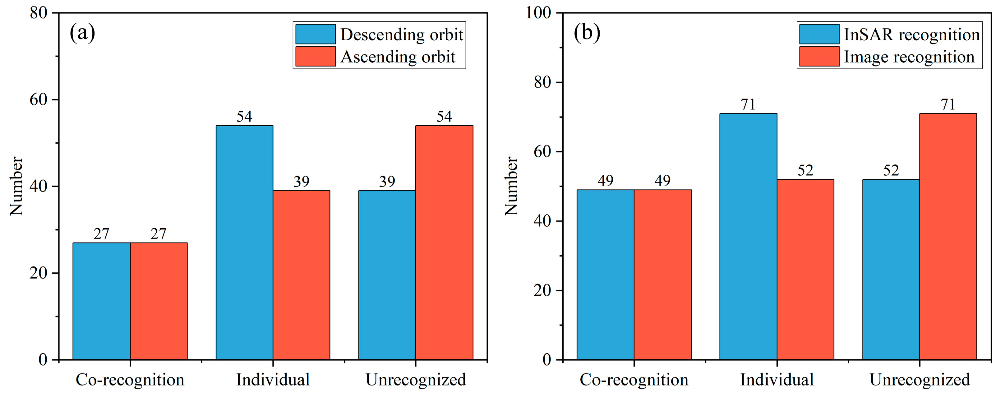
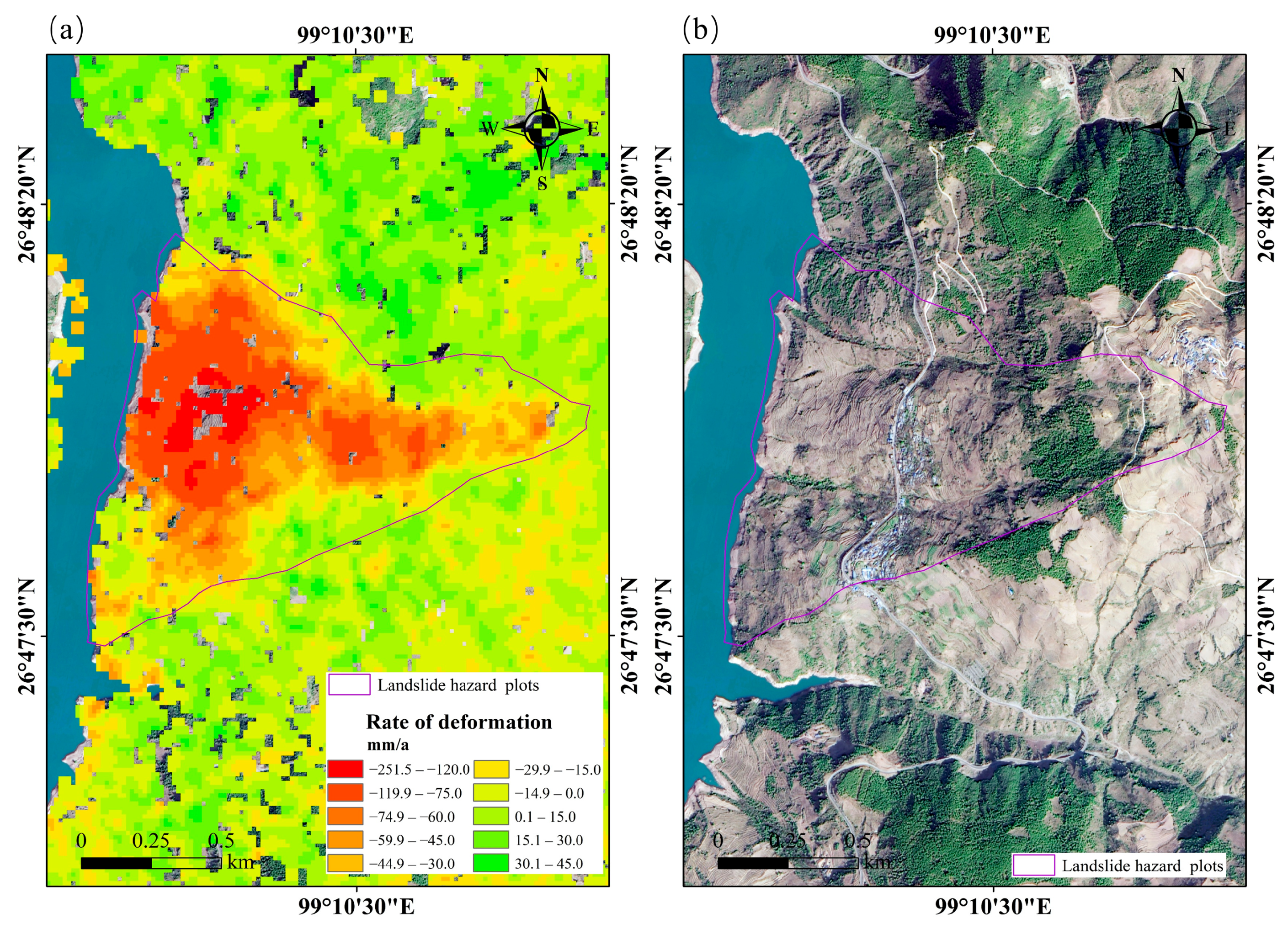
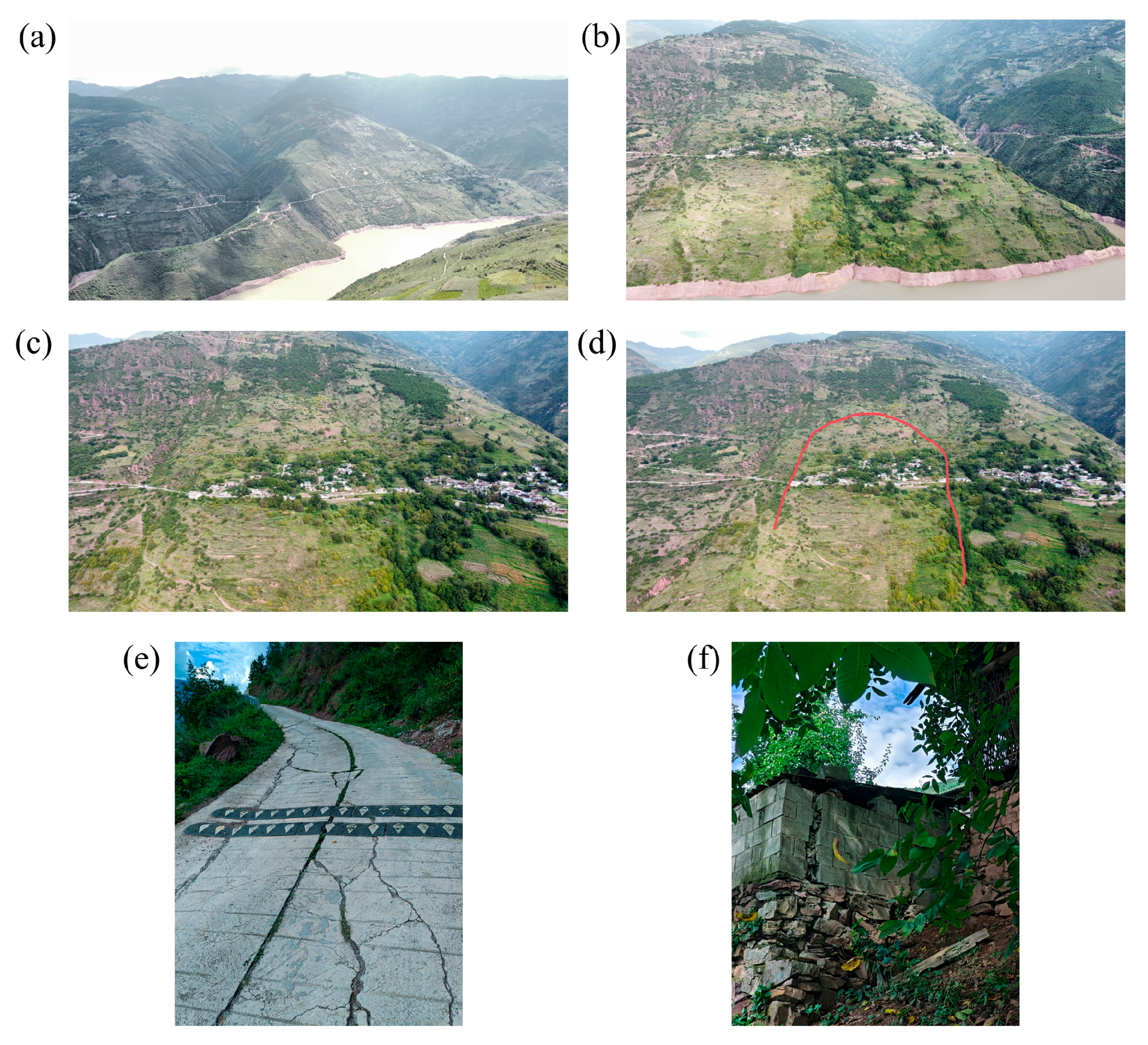
The joint method used in this paper effectively overcomes the limitations of optical imagery, which is susceptible to weather and has difficulty monitoring landslides in deformed areas, and reduces the impact of single-orbit radar satellite identification errors in high mountain canyon areas. Through UAV aerial photography and on-site validation, the study found that the landslide hazards in Cheyiping are more serious and that there are many residents living in this vulnerable area than had previously been. Therefore, it is of great practical significance to carry out early identification of landslides in high mountain valley areas for disaster prevention and mitigation, and for the protection of people’s lives and properties.

However, this study still has some limitations. First, the C-band radar data used in the research has limited penetration capability in areas with dense vegetation, resulting in less effective landslide hazard identification in some regions. To improve the accuracy of InSAR monitoring, future studies will consider incorporating L-band radar data, such as LuTan data, which has stronger penetration capabilities compared to C-band radar and can more effectively address landslide identification challenges in complex surface conditions. Second, it should be noted that, during the field validation of landslide hazards, we only selected a few representative areas for on-site investigation. This selection may not have comprehensively covered all types of landslide risks within the region. Therefore, future studies will expand the scope of field validation in high mountains, deep valleys, and areas with complex geological conditions, and will consider using high-resolution remote-sensing technologies such as LiDAR for more precise terrain and deformation monitoring. This will further improve the accuracy of the landslide hazard identification.

5.2. Screening and Risk Zoning of Landslide Disaster-Inducing Factors

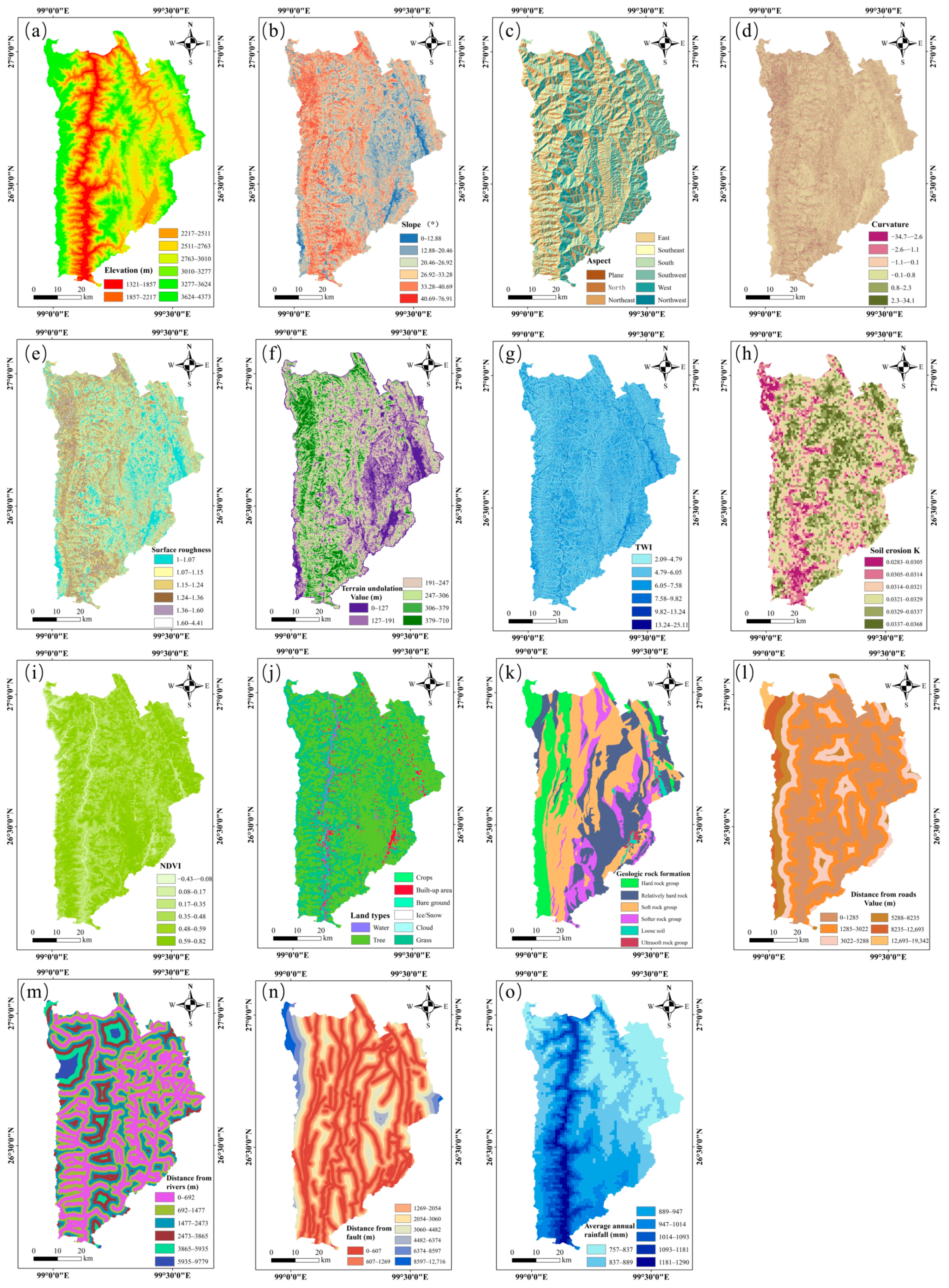
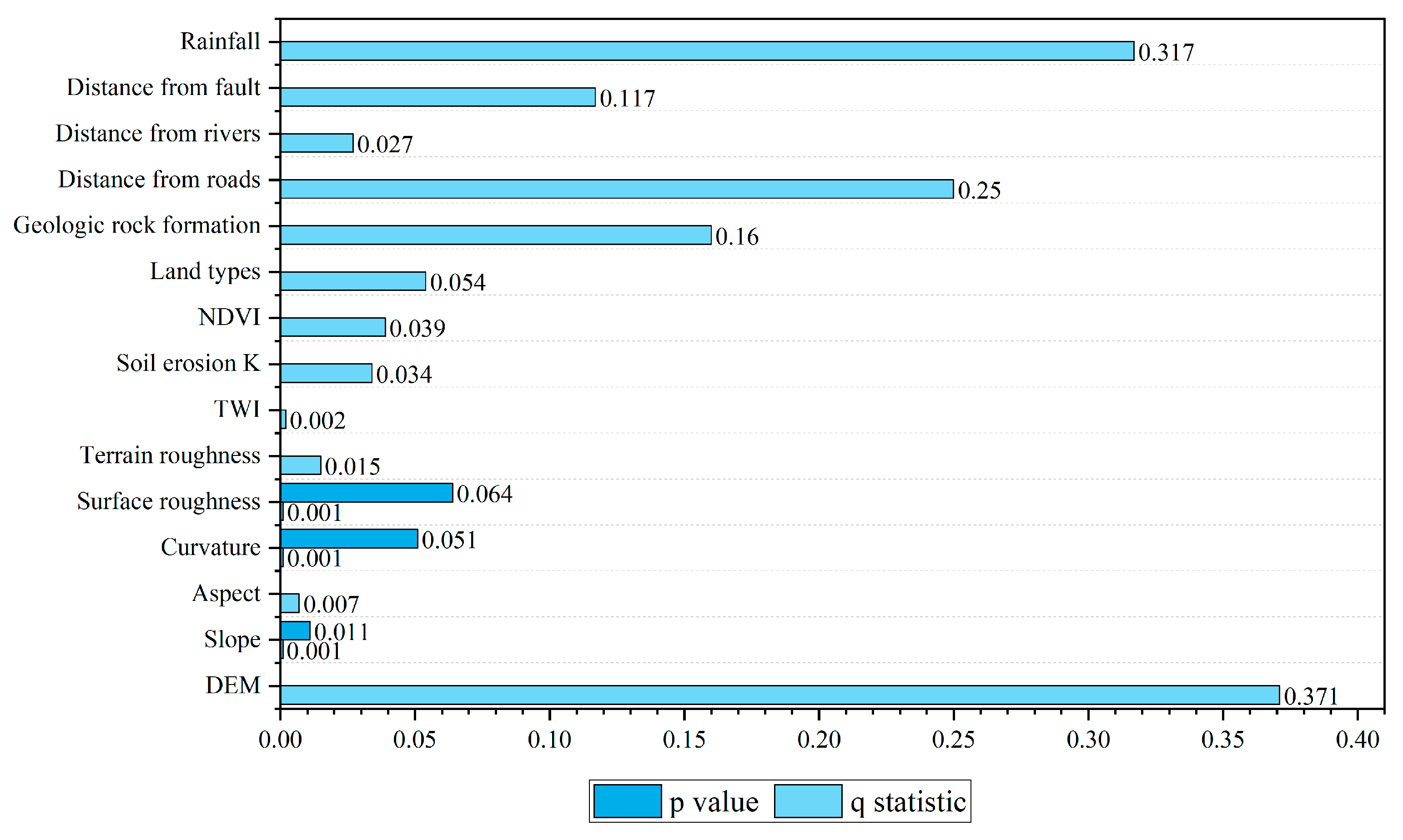
The selection of landslide predisposing factors is usually based on the combined effects of natural conditions and human activities on landslide occurrence. Currently, many scholars rely only on expert experience to obtain indicator factors for sensitivity studies, without exploring whether the factors have provided sufficient contributions to the evaluation and the division of the factor risk zones. This expert experience has affected our ability to discriminate landslide-inducing factors in a specific area. This study fully leverages the advantages of the geodetector method, which not only identifies significant disaster-inducing factors for landslides from the examination and use of vast datasets but also is able to distinguish high-risk factor intervals. With the factor detector, we found that landslides exhibit stronger significance in factors such as DEM, rainfall, distance from roads, and geological rock formation. However, there were factors like curvature and surface roughness that did not pass the significance test and should, therefore, be excluded.

DEM primarily affects the probability of landslide occurrence indirectly through terrain, slope, climate, and vegetation conditions. Areas at a certain altitude are typically characterized by steeper slopes, enhanced gravitational forces, and a higher likelihood of instability in the rock and soil masses. Therefore, in mountainous areas, landslide occurrences are typically closely related to specific elevation conditions. Rainfall increases the infiltration of water on slopes, which reduces the friction coefficient between weak zones, thereby weakening the shear strength of these zones and promoting slope failure. Additionally, the distance from main roads is often used as an indicator of human engineering activity. Roads built on slopes disrupt the support structure at the base of the slope, and as terrain changes and support is lost, cracks may form and expand. When moisture further infiltrates the slope, it can eventually lead to instability. The differences in the properties of engineering geological rock formation, such as rock composition, hardness, and degree of weathering and fracturing, determine the development characteristics of landslides.

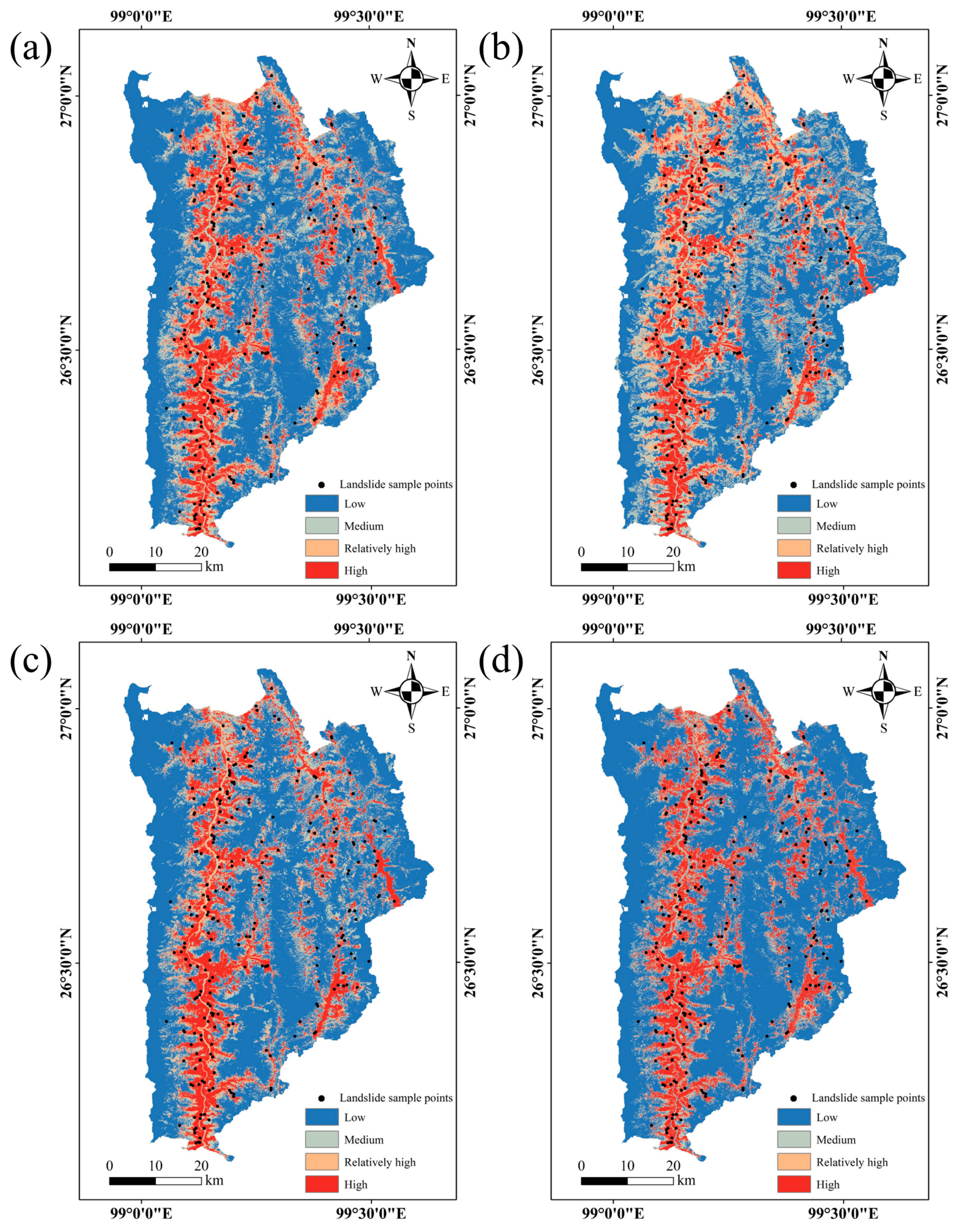
The factor detector takes the above factors as the most important influencing factors, which does not mean that the role of other important factors, such as side slopes, is neglected. Whereas landslides are often caused by the interaction of multiple factors, in the interaction detector results, we can find that the combined effect of slope, DEM, and other factors can have higher explanatory power. Therefore, it is more reasonable to assume that it is probable that we can derive the higher sensitivity of landslides to the above-mentioned significant disaster-inducing factors through the use of geodetector. Finally, through the analysis of the risk detector, we were also able to determine the distribution of the risk intervals of landslides with respect to the risk factors of the breeding factors. This analysis provides important insights for the identification and risk assessment of different types of landslides and can help guide the formulation of landslide mitigation and prevention measures.

5.3. Demonstration Study on the Sensitivity Evaluation of Small Samples of Landslides

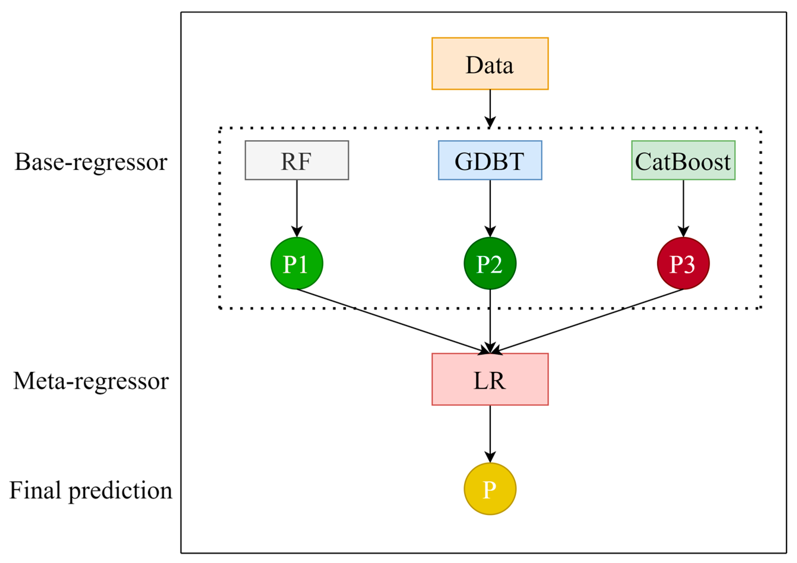
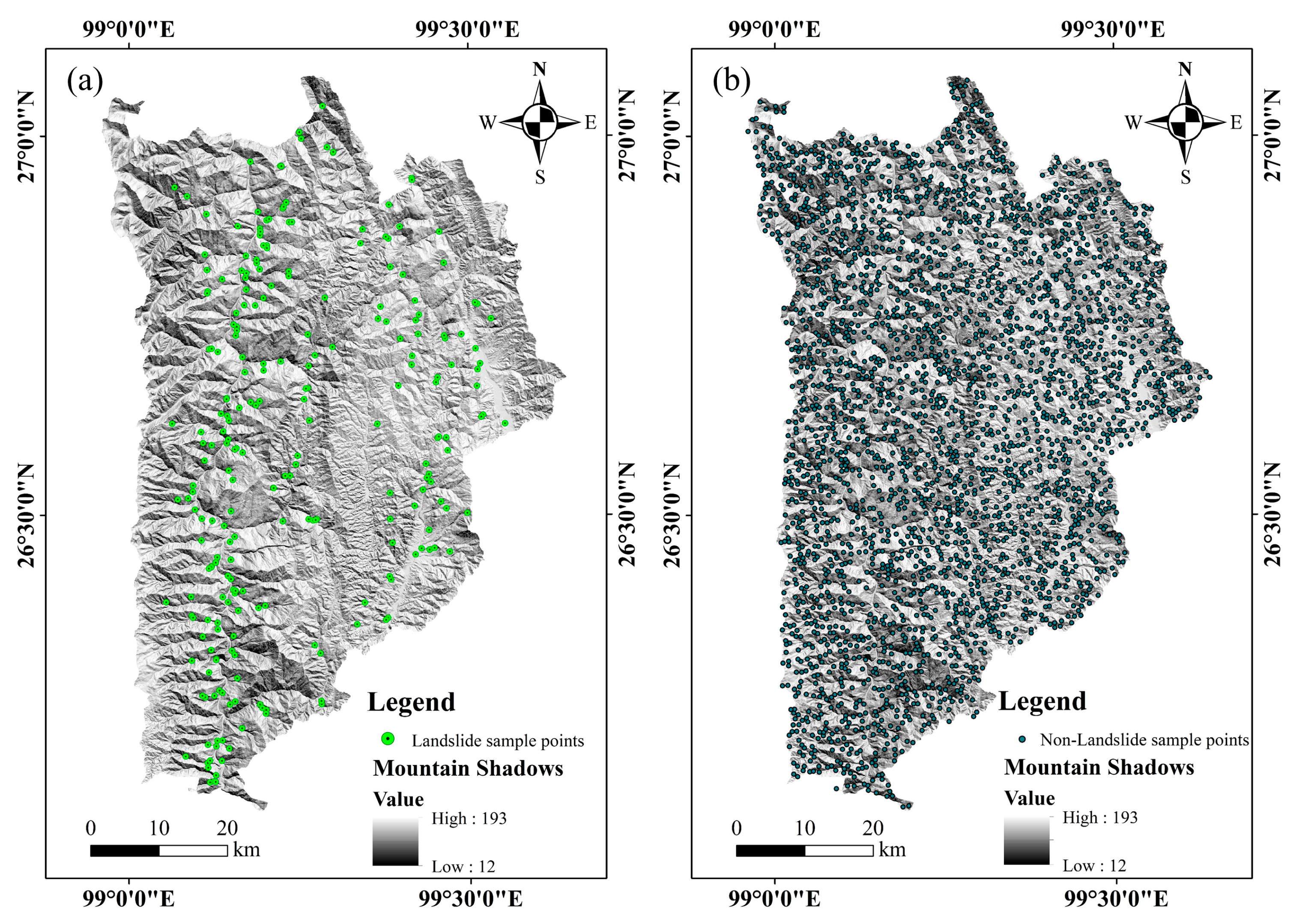
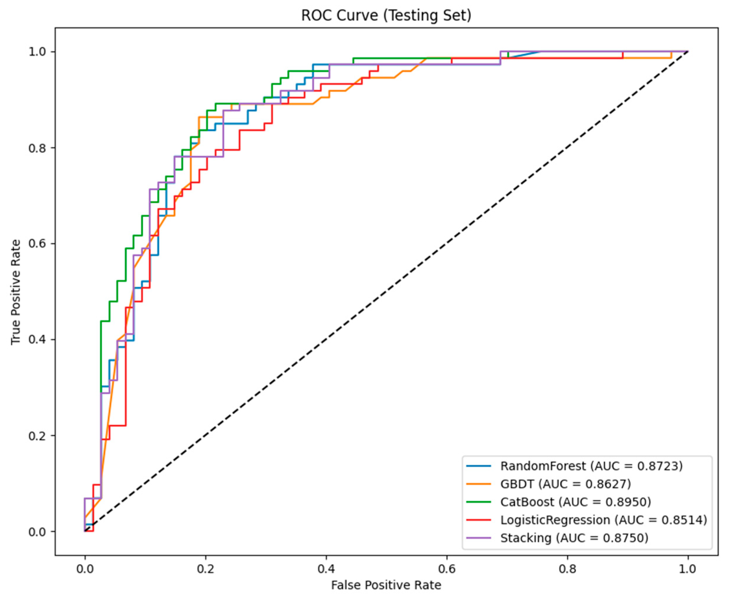
This study selected 13 disaster-inducing factors based on geodetector and used RF, GBDT, CatBoost, LR, and stacking algorithms for landslide sensitivity evaluation. For sample selection, we innovatively applied the K-means clustering algorithm to optimize non-landslide samples, ensuring the scientific and rational design of the experiment. In our model optimization, Bayesian optimization was used for hyperparameter tuning to minimize the impact of human intervention on model performance. The experimental results show that all four models performed well, with the GD-CatBoost model achieving the highest accuracy.

However, the study area is relatively limited, with only 245 landslide samples. We conducted an extensive selection and comparison of the learning algorithms. An initial attempt was made using the Tab-Transformer deep-learning model for landslide sensitivity evaluation, but the experimental results indicated that the model performed poorly, mainly due to the limited number of landslide samples. Although deep-learning methods have shown promising results in landslide sensitivity evaluations, this study indicates that, under small sample conditions, the GD-CatBoost model is an excellent classification tool that can effectively distinguish and identify potentially sensitive areas for landslide occurrence.

In future research, we expect to expand the landslide sample size to further incorporate the application of deep-learning models (Transformer, CNN-LSTM, etc.) through in-depth studies of large landslide areas in order to improve the evaluation precision and accuracy under small sample conditions.

6. Conclusions

The main conclusions are as follows.

(1)

By integrating high-resolution optical imagery, the SBAS-InSAR technique was employed to detect landslide hazards in mountainous regions utilizing both ascending and descending orbit data. A total of 172 landslide hazards were identified. In terms of spatial distribution, the identified landslide-prone areas are predominantly concentrated along the banks of the Lancang River valleys;

(2)

The geodetector method elucidates the significance and risk intervals of the disaster-inducing factors of landslide formation by detailing the characteristics of the indicator factors. The significant disaster-inducing factors and risk intervals of landslides in the Lanping area mainly include DEM (1321–1857 m), rainfall (1181–1290 mm), distance from the road (0–1285 m), and geological rock formation (soft rock formation). The difference in the result that we obtained with the explanatory power of each single factor indicates that there is a significant difference in the sensitivity of the causation of landslides with different factors;

(3)

Based on the K-means clustering algorithm for non-landslide sample optimization and the Bayesian algorithm to find optimal parameters, the GD-CatBoost model demonstrates excellent performance. The model achieved an AUC of 0.895, an F1 score of 0.8421, a recall of 0.8776, and a Kappa value of 0.6736. The spatial analysis of landslide sensitivity shows that the highly sensitive areas are mainly located along the banks of the Lancang River. The percentage of high and relatively high sensitive areas for landslides reaches 24.2%. These findings suggest that, in the Lamping County area, deeply cut valley areas affected by topographic elevation differences and river erosion are particularly sensitive to landslides.

This study elucidates the spatial distribution of landslide sensitivity, effectively addressing the challenge of recognizing landslide hazards and understanding the complex interactions of triggering factors in complex mountainous areas. The small-sample sensitivity evaluation framework for landslides that we developed helps qualitatively and quantitatively examine the potential mechanisms of landslides in these regions from local, global, and spatial perspectives.

References

1. Zeng, T.; Jin, B.; Glade, T.; Xie, Y.; Li, Y.; Zhu, Y.; Yin, K. Assessing the imperative of conditioning factor grading in machine learning-based landslide susceptibility modeling: A critical inquiry. Catena 2024, 236, 107732. [Google Scholar] [CrossRef]
2. Li, Y.; Deng, X.; Ji, P.; Yang, Y.; Jiang, W.; Zhao, Z. Evaluation of landslide susceptibility based on CF-SVM in Nujiang Prefecture. Int. J. Environ. Res. Public Health 2022, 19, 14248. [Google Scholar] [CrossRef]
3. Sharma, N.; Saharia, M.; Ramana, G.V. High resolution landslide susceptibility mapping using ensemble machine learning and geospatial big data. Catena 2024, 235, 107653. [Google Scholar] [CrossRef]
4. Huang, F.; Xiong, H.; Jiang, S.-H.; Yao, C.; Fan, X.; Catani, F.; Chang, Z.; Zhou, X.; Huang, J.; Liu, K. Modelling landslide susceptibility prediction: A review and construction of semi-supervised imbalanced theory. Earth-Sci. Rev. 2024, 250, 104700. [Google Scholar] [CrossRef]
5. Liu, X.; Zhao, C.; Yin, Y.; Tomás, R.; Zhang, J.; Zhang, Q.; Wei, Y.; Wang, M.; Lopez-Sanchez, J.M. Refined InSAR method for mapping and classification of active landslides in a high mountain region: Deqin County, southern Tibet Plateau, China. Remote Sens. Environ. 2024, 304, 114030. [Google Scholar] [CrossRef]
6. Macciotta, R.; Hendry, M.T. Remote sensing applications for landslide monitoring and investigation in western Canada. Remote Sens. 2021, 13, 366. [Google Scholar] [CrossRef]
7. Jaboyedoff, M.; Oppikofer, T.; Abellán, A.; Derron, M.-H.; Loye, A.; Metzger, R.; Pedrazzini, A. Use of LIDAR in landslide investigations: A review. Nat. Hazards 2012, 61, 5–28. [Google Scholar] [CrossRef]
8. Zhao, C.; Lu, Z. Remote sensing of landslides—A review. Remote Sens. 2018, 10, 279. [Google Scholar] [CrossRef]
9. Casagli, N.; Intrieri, E.; Tofani, V.; Gigli, G.; Raspini, F. Landslide detection, monitoring and prediction with remote-sensing techniques. Nat. Rev. Earth Environ. 2023, 4, 51–64. [Google Scholar] [CrossRef]
10. González, P.J. Interferometric Synthetic Aperture Radar (InSAR). In Remote Sensing for Characterization of Geohazards and Natural Resources; Springer International Publishing: Cham, Switzerland, 2024; pp. 53–73. [Google Scholar] [CrossRef]
11. Ferretti, A.; Prati, C.; Rocca, F. Permanent scatterers in SAR interferometry. IEEE Trans. Geosci. Remote Sens. 2002, 39, 8–20. [Google Scholar] [CrossRef]
12. Berardino, P.; Fornaro, G.; Lanari, R.; Sansosti, E. A new algorithm for surface deformation monitoring based on small baseline differential SAR interferograms. IEEE Trans. Geosci. Remote Sens. 2002, 40, 2375–2383. [Google Scholar] [CrossRef]
13. Ye, X.; Kaufmann, H.; Guo, X.F. Landslide monitoring in the Three Gorges area using D-InSAR and corner reflectors. Photogramm. Eng. Remote Sens. 2004, 70, 1167–1172. [Google Scholar] [CrossRef]
14. Chen, Y.; Yu, S.; Tao, Q.; Liu, G.; Wang, L.; Wang, F. Accuracy verification and correction of D-InSAR and SBAS-InSAR in monitoring mining surface subsidence. Remote Sens. 2021, 13, 4365. [Google Scholar] [CrossRef]
15. Chen, X.; Tessari, G.; Fabris, M.; Achilli, V.; Floris, M. Comparison between PS and SBAS InSAR techniques in monitoring shallow landslides. In Understanding and Reducing Landslide Disaster Risk: Volume 3 Monitoring and Early Warning 5th; Springer: Cham, Switzerland, 2021; pp. 155–161. [Google Scholar] [CrossRef]
16. Dong, J.; Niu, R.; Li, B.; Xu, H.; Wang, S. Potential landslides identification based on temporal and spatial filtering of SBAS-InSAR results. Geomat. Nat. Hazards Risk 2023, 14, 52–75. [Google Scholar] [CrossRef]
17. Kulsoom, I.; Hua, W.; Hussain, S.; Chen, Q.; Khan, G.; Shihao, D. SBAS-InSAR based validated landslide susceptibility mapping along the Karakoram Highway: A case study of Gilgit-Baltistan, Pakistan. Sci. Rep. 2023, 13, 3344. [Google Scholar] [CrossRef]
18. Quevedo, R.P.; Velastegui-Montoya, A.; Montalván-Burbano, N.; Morante-Carballo, F.; Korup, O.; Rennó, C.D. Land use and land cover as a conditioning factor in landslide susceptibility: A literature review. Landslides 2023, 20, 967–982. [Google Scholar] [CrossRef]
19. McColl, S.T. Landslide causes and triggers. In Landslide Hazards, Risks, and Disasters; Elsevier: Amsterdam, The Netherlands, 2022; pp. 13–41. [Google Scholar] [CrossRef]
20. Sun, D.; Shi, S.; Wen, H.; Xu, J.; Zhou, X.; Wu, J. A hybrid optimization method of factor screening predicated on GeoDetector and Random Forest for Landslide Susceptibility Mapping. Geomorphology 2021, 379, 107623. [Google Scholar] [CrossRef]
21. Merghadi, A.; Yunus, A.P.; Dou, J.; Whiteley, J.; ThaiPham, B.; Bui, D.T.; Avtar, R.; Abderrahmane, B. l Machine learning methods for landslide susceptibility studies: A comparative overview of algorithm performance. Earth-Sci. Rev. 2020, 207, 103225. [Google Scholar] [CrossRef]
22. Azarafza, M.; Azarafza, M.; Akgün, H.; Atkinson, P.M.; Derakhshani, R. Deep learning-based landslide susceptibility mapping. Sci. Rep. 2021, 11, 24112. [Google Scholar] [CrossRef]
23. Taalab, K.; Cheng, T.; Zhang, Y. Mapping landslide susceptibility and types using Random Forest. Big Earth Data 2018, 2, 159–178. [Google Scholar] [CrossRef]
24. Gu, T.; Duan, P.; Wang, M.; Li, J.; Zhang, Y. Effects of non-landslide sampling strategies on machine learning models in landslide susceptibility mapping. Sci. Rep. 2024, 14, 7201. [Google Scholar] [CrossRef] [PubMed]
25. Akgun, A. A comparison of landslide susceptibility maps produced by logistic regression, multi-criteria decision, and likelihood ratio methods: A case study at İzmir, Turkey. Landslides 2012, 9, 93–106. [Google Scholar] [CrossRef]
26. Huan, Y.; Song, L.; Khan, U.; Zhang, B. Stacking ensemble of machine learning methods for landslide susceptibility mapping in Zhangjiajie City, Hunan Province, China. Environ. Earth Sci. 2023, 82, 35. [Google Scholar] [CrossRef]
27. Lee, S.M.; Lee, S.J. Landslide susceptibility assessment of South Korea using stacking ensemble machine learning. Geoenviron. Disasters 2024, 11, 7. [Google Scholar] [CrossRef]
28. Alqadhi, S.; Mallick, J.; Alkahtani, M.; Ahmad, I.; Alqahtani, D.; Hang, H.T. Developing a hybrid deep learning model with explainable artificial intelligence (XAI) for enhanced landslide susceptibility modeling and management. Nat. Hazards 2024, 120, 3719–3747. [Google Scholar] [CrossRef]
29. Zhang, X.; Gan, S.; Yuan, X.; Zong, H.; Wu, X. Slope deformation monitoring and early identification of disasters in debris flow source area of Baini River, Dongchuan District, China. Front. Earth Sci. 2022, 10, 1000736. [Google Scholar] [CrossRef]
30. Chen, Y.; Dong, J.; Guo, F.; Tong, B.; Zhou, T.; Fang, H.; Wang, L.; Zhang, Q. Review of landslide susceptibility assessment based on knowledge mapping. Stoch. Environ. Res. Risk Assess. 2022, 36, 2399–2417. [Google Scholar] [CrossRef]
31. Wang, J.; Xu, C. Geodetector: Principle and prospective. Acta Geogr. Sin. 2017, 72, 116–134. [Google Scholar] [CrossRef]
32. Li, Z.; Zhao, Z.; Zhang, T. Livability evaluation of urban environment based on Google Earth Engine and multi-source data: A case study of Kunming, China. Ecol. Indic. 2024, 169, 112968. [Google Scholar] [CrossRef]
33. Ullah, M.I.; Aslam, M.; Altaf, S.; Ahmed, M. Some new diagnostics of multicollinearity in linear regression model. Sains Malays. 2019, 48, 2051–2060. [Google Scholar] [CrossRef]
34. Breiman, L. Random forests. Mach. Learn. 2001, 45, 5–32. [Google Scholar] [CrossRef]
35. Hancock, J.T.; Khoshgoftaar, T.M. CatBoost for big data: An interdisciplinary review. J. Big Data 2020, 7, 94. [Google Scholar] [CrossRef] [PubMed]
36. Ran, X.; Suyaroj, N.; Tepsan, W.; Ma, J.; Zhou, X.; Deng, W. A hybrid genetic-fuzzy ant colony optimization algorithm for automatic K-means clustering in urban global positioning system. Eng. Appl. Artif. Intell. 2024, 137, 109237. [Google Scholar] [CrossRef]
37. Xiao, X.; Zou, Y.; Huang, J.; Luo, X.; Yang, L.; Li, M.; Yang, P.; Ji, X.; Li, Y. An interpretable model for landslide susceptibility assessment based on Optuna hyperparameter optimization and Random Forest. Geomat. Nat. Hazards Risk 2024, 15, 2347421. [Google Scholar] [CrossRef]
38. Heydarian, M.; Doyle, T.E.; Samavi, R. MLCM: Multi-label confusion matrix. IEEE Access 2022, 10, 19083–19095. [Google Scholar] [CrossRef]
39. Muschelli, J., III. ROC and AUC with a binary predictor: A potentially misleading metric. J. Classif. 2020, 37, 696–708. [Google Scholar] [CrossRef]
40. Babitha, B.G.; Danumah, J.H.; Pradeep, G.S.; Costache, R.; Patel, N.; Prasad, M.K.; Rajaneesh, A.; Mammen, P.C.; Ajin, R.S.; Kuriakose, S.L. A framework employing the AHP and FR methods to assess the landslide susceptibility of the Western Ghats region in Kollam district. Saf. Extrem. Environ. 2022, 4, 171–191. [Google Scholar] [CrossRef]
Figure 1. Study area location map.
Remotesensing 17 01634 g001
Figure 2. Route map.
Remotesensing 17 01634 g002
Figure 3. SBAS-InSAR flow chart.
Remotesensing 17 01634 g003
Figure 4. Indicator factors. (ao) represents respectively the resultant plots after reclassification of the, DEM, slope, aspect, curvature, surface roughness, terrain roughness, TWI, soil erosion K, NDVI, land types, geologic rock formation, distance from roads, distance from rivers, distance from fault, and rainfall.
Remotesensing 17 01634 g004
Figure 5. Stacking flow chart.
Remotesensing 17 01634 g005
Figure 6. Annual average deformation rate: (a) descending and (b) ascending.
Remotesensing 17 01634 g006
Figure 7. Histogram of the number of landslide hazards identified, where (a) indicates the number of ascending and descending orbit identifications in the InSAR data, and (b) indicates the number of InSAR and optical identifications.
Remotesensing 17 01634 g007
Figure 8. Cheyiping landslide: (a) deformation rate graph; (b): GF-2 imagery.
Remotesensing 17 01634 g008
Figure 9. Cheyiping landslide drone and site verification photos. (ad) are drone aerial photos, (e,f) are photos of local landslide signs.
Remotesensing 17 01634 g009
Figure 10. (a,b) Distributions represent landslide sample points and non-landslide sample points.
Remotesensing 17 01634 g010
Figure 11. One-factor explanatory power.
Remotesensing 17 01634 g011
Figure 12. Interaction factor explanatory power. A–O represent, respectively, DEM, slope, aspect, curvature, surface roughness, terrain roughness, TWI, soil erosion K, NDVI, land types, geologic rock formation, distance from roads, distance from rivers, distance from fault, and rainfall.
Remotesensing 17 01634 g012
Figure 13. ROC and AUC results.
Remotesensing 17 01634 g013
Figure 14. Mapping of landslide-sensitive areas. (ad) represent, respectively, RF, GDBT, CatBoost, and stacking results.
Remotesensing 17 01634 g014