Long-Term (2015–2024) Daily PM_2.5 Estimation in China by Using XGBoost Combining Empirical Orthogonal Function Decomposition

Abstract

Fine particulate matter (PM_2.5) has garnered significant scientific and public health concern owing to its capacity for deep penetration into the human respiratory system, presenting significant health risks. Despite the implementation of strict environmental policies in China over the past decade to reduce PM_2.5 levels, long-term public health concerns remain a serious issue. Our study aims to provide a high-quality, seamless daily PM_2.5 dataset for China covering the years 2015 to 2024. A two-step PM_2.5 estimation model is established based on a machine learning algorithm and a spatio-temporal decomposition method. First, we utilize the machine learning algorithm XGBoost (EXtreme Gradient Boosting) to address gaps in the daily MAIAC (Multi-Angle Implementation of Atmospheric Correction) AOD (Aerosol Optical Depth), with R²/RMSE (coefficient of determination/Root Mean Square Error) of 0.67/0.2678 compared to AERONET (Aerosol Robotic Network) AOD. Then, a novel approach by integrating XGBoost with EOF (Empirical Orthogonal Function) decomposition is introduced for PM_2.5 estimation. The integration of EOF allows for the incorporation of entire meteorological field information into the PM_2.5 estimation model, significantly enhancing its accuracy: spatial CV (cross-validation)-R² improved from 0.8340 to 0.8935, and spatial CV-RMSE reduced from 13.8177 to 11.0668. Leveraging the newly produced dataset, we analyze the spatio-temporal variations of PM_2.5 across China with EOF decomposition, particularly noting that PM_2.5 levels in the eastern anthropogenic intensive regions continuously declined from 2015 to 2020, and fluctuated steadily during 2020–2024. This research underscores the critical need for sustained and effective air quality management strategies in China.

1. Introduction

Over the past decades, rapid industrialization and urbanization across China have led to serious air pollution, significantly affecting human health and the environment [1,2,3]. For example, fine particulate matter (PM_2.5), a type of particulate matter characterized by an aerodynamic diameter of less than 2.5 μm, bears the capability for deep penetration into the alveolar regions of the human respiratory system and enters the human circulatory system, thereby inducing respiratory [4] and cardiovascular diseases [5]. To address this issue, the Chinese government implemented two key policies: the “Air Pollution Prevention and Control Action Plan” in 2013 [6] and the “Three-Year Action Plan for Winning the Blue Sky” in 2018 [7]. These policies have significantly reduced regional PM_2.5 levels [8,9,10]. However, severe haze events in northern Chinese cities during the winters over the past decade still underscore the persistent threat of PM_2.5 to public health. Hence, accurately assessing the spatio-temporal distribution of PM_2.5 is essential for crafting effective air quality management policies and safeguarding public health.

Surface PM_2.5 monitoring mainly relies on ground stations, but their sparse distribution makes it challenging to accurately represent PM_2.5 concentrations across large areas [11,12,13]. To address this limitation, previous research [14,15,16,17,18] has proposed various statistical models to estimate the regional or global PM_2.5 distribution. Early studies typically employed a simple linear regression model to parameterize the association between satellite-derived AOD and PM_2.5 concentrations from in situ measurements [19,20]. However, these models did not consider the influence of meteorological conditions, which limited their accuracy. To overcome this problem, researchers have incorporated meteorological data into multivariable linear regression frameworks, enabling enhanced quantification of the AOD-PM_2.5 relationship through explicit modeling of aerosol hygroscopic growth and vertical mixing effects [21,22,23]. Additionally, advancements in machine learning and deep learning algorithms have introduced techniques such as Support Vector Machines [24], Random Forests [25], and Deep Neural Networks [26] to estimate PM_2.5 concentrations, resulting in high-quality PM_2.5 datasets.

Meteorological factors, such as temperature, humidity, and wind velocity vectors (which can be decomposed into the speed and direction of wind), exert critical modulation in the formation, dispersion, and deposition of surface PM_2.5 [27,28,29,30]. Previous research has demonstrated that multivariate regression models incorporating meteorological variables perform better than simple linear models that rely solely on satellite-derived AOD. Recent studies [31,32,33] emphasized the importance of integrating the whole meteorological field information to enhance the accuracy of PM_2.5 estimation models. Techniques, such as wavelet decomposition, which capture meteorological changes across different time scales, have proven effective in revealing the complex relationships between these variables and PM_2.5 levels, significantly improving the estimation model accuracy. Similarly, empirical orthogonal function (EOF) decomposition could extract the main modes of the meteorological field [34,35,36] and has the potential to significantly improve estimation accuracy.

Our study aims to develop a comprehensive, high-quality daily PM_2.5 dataset across China from 2015 to 2024, employing EOF decomposition and the machine learning algorithm XGBoost. Our research consists of several tasks: (1) utilizing XGBoost to address gaps in daily MAIAC AOD; (2) incorporating the whole meteorological field information into the PM_2.5 estimation model through EOF decomposition, and producing daily PM_2.5 data across China covering the years 2015 to 2024; (3) integrating population data to compute trends in population-weighted PM_2.5 changes; (4) analyzing the spatio-temporal variations of PM_2.5 using EOF decomposition. Section 2 outlines the datasets utilized and the methodology for PM_2.5 estimation, while Section 3 systematically analyzes the derived seamless AOD and PM_2.5 distributions through multi-scale temporal (annual/seasonal/monthly) and spatial (regional/urban–rural) evaluations. Building upon these findings, Section 4 provides a critical discussion on possible drivers of the PM_2.5 pattern, while Section 5 draws conclusions systematically.

2. Materials and Methods

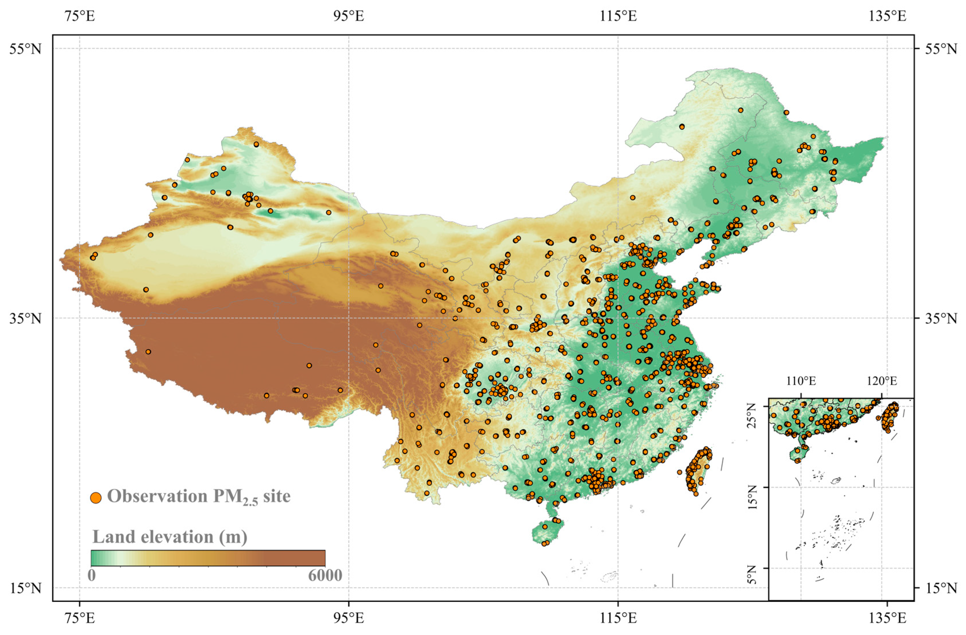
2.1. Study Region

China, the largest developing nation globally, exhibits extensive geographic and climatic diversity (as shown in Figure 1). With rapid industrialization and urbanization, air pollution has significantly deteriorated, posing serious threats to public health. In response, the Chinese government has established and continuously maintained a nationwide air pollution monitoring network and publicly releases pollutant concentrations (including PM_2.5) on time. These efforts, combined with enacted a range of strict environmental policies, including industrial emission standards [37] and urban greening initiatives [38], have collectively contributed to the mitigation of air pollution across China. While these actions and policies have improved air quality significantly, PM_2.5 remains a major health issue in highly industrialized regions.

2.2. Datasets

2.2.1. PM_2.5 Station Data

Our study utilizes hourly PM_2.5 observation records from CNEMC (China National Environmental Monitoring Centre, http://www.cnemc.cn/ (accessed on 1 May 2025)) and the Environmental Protection Administration of Taiwan (https://data.moenv.gov.tw/en/ (accessed on 1 May 2025)). These records span from 2015 to 2024 and encompass 2025 monitoring sites, including 87 in Taiwan. The locations of these sites are illustrated in Figure 1.

2.2.2. AOD Data

The MODIS (Moderate Resolution Imaging Spectroradiometer) daily MAIAC AOD provides AOD using 1 km × 1 km grids (https://ladsweb.modaps.eosdis.nasa.gov/ (accessed on 1 May 2025)) and is produced by NASA (National Aeronautics and Space Administration) using the MAIAC algorithm [39,40,41]. This algorithm processes observations from the MODIS payload onboard the Terra and Aqua satellites. The spatial gaps exist in MAIAC AOD due to factors such as clouds, precipitation, and satellite revisit intervals, which hinder its application in regional gapless pollutant estimation.

The MERRA-2 (Modern-Era Retrospective analysis for Research and Applications Version 2) AOD dataset (https://disc.gsfc.nasa.gov/datasets/ (accessed on 1 May 2025)), part of NASA MERRA-2 data, provides hourly global AOD with a spatial resolution of 0.5° × 0.625° [42,43,44]. Spatial gapless as it is, the relatively coarse spatial resolution it bears limits its ability to resolve the spatial heterogeneity of atmospheric pollution, making it less suitable for fine-scale characterization compared to MAIAC AOD.

AERONET (available at https://aeronet.gsfc.nasa.gov/ (accessed on 1 May 2025)) is a global network of sun photometers that measure the optical properties of atmospheric aerosols [45]. These measurements are taken under clear-sky conditions and are used to study the spatio-temporal variability of aerosols, their impact on climate, and their role in air quality. AERONET AOD is widely used in the validation of satellite-based AOD products. However, AERONET data at 550 nm is not directly available. To overcome this constraint, we employed a quadratic polynomial interpolation approach [46], utilizing AOD measurements at 440 nm, 500 nm, and 675 nm to simulate the AOD at 550 nm. The interpolation formula is expressed as follows:

$$\ln {\tau }_{\lambda }=a_0+a_1\ln \lambda +a_2{(\ln \lambda )}^2$$

(1)

where ${\tau }_{\lambda }$ represents the AERONET-observed AOD at λ nm, and $a_0$, $a_1$, $a_2$ denote unknown parameters derived through constrained nonlinear optimization of the AERONET AOD measurements at 440 nm, 500 nm, and 675 nm.

2.2.3. Meteorological Fields

The ERA5 (European Centre for Medium-Range Weather Forecast (ECMWF) Reanalysis v5) Single Level dataset (https://cds.climate.copernicus.eu/ (accessed on 1 May 2025)), a key component of the ECMWF global weather and climate reanalysis project, provides hourly global atmospheric data using 0.25° × 0.25° grids [47,48]. The ERA5 dataset encompasses a comprehensive array of meteorological variables, including temperature, humidity, wind speed, and pressure across different atmospheric levels. This study will utilize parameters that are critical for AOD reconstruction and PM_2.5 estimation, such as boundary layer dynamics (boundary layer height (blh) and surface pressure (sp)), hydrometeorological parameters (total column water (tcw), relative humidity (rh) and total precipitation (tp)), aerodynamic forcing parameters (the zonal wind components at 10 m elevation (u10) and the meridional wind components at 10 m elevation (v10)) and thermodynamic state parameters (air temperature at 2 m elevation (t2 m)).

2.2.4. Additional Data

The SRTM (Shuttle Radar Topography Mission) DEM (Digital Elevation Model), created by NASA, is a high-resolution global topographic dataset derived from radar measurements aboard the Space Shuttle. It offers elevation data with a spatial resolution of approximately 30 m, covering the land surface between 60° north and 56° south latitude of the Earth. This dataset is integral to GIS (Geographic Information Systems), remote sensing, and various other scientific and engineering applications, including terrain analysis, flood modeling, and infrastructure planning [49]. We downloaded the SRTM DEM across China with a spatial resolution of 1 km × 1 km grid from the Resource and Environmental Science Data Platform (https://www.resdc.cn/ (accessed on 1 May 2025)).

The LandScan Global Population Dataset, developed and released by ORNL (Oak Ridge National Laboratory), is a high-resolution model designed to estimate population distribution [50]. It provides population counts using 30 arc-second × 30 arc-second grids (1 km × 1 km grids approximately) worldwide. LandScan plays a crucial role in disaster response, public health research, and environmental impact assessments. The dataset is updated annually and freely available from ORNL (https://landscan.ornl.gov/ (accessed on 1 May 2025)). Since the 2024 LandScan data have not yet been released, this study utilizes China’s total population data from the Population Pyramid (https://www.populationpyramid.net/ (accessed on 1 May 2025)) to make linear adjustments to the 2023 LandScan dataset, thereby estimating China’s population distribution for 2024.

2.2.5. Data Reprocessing

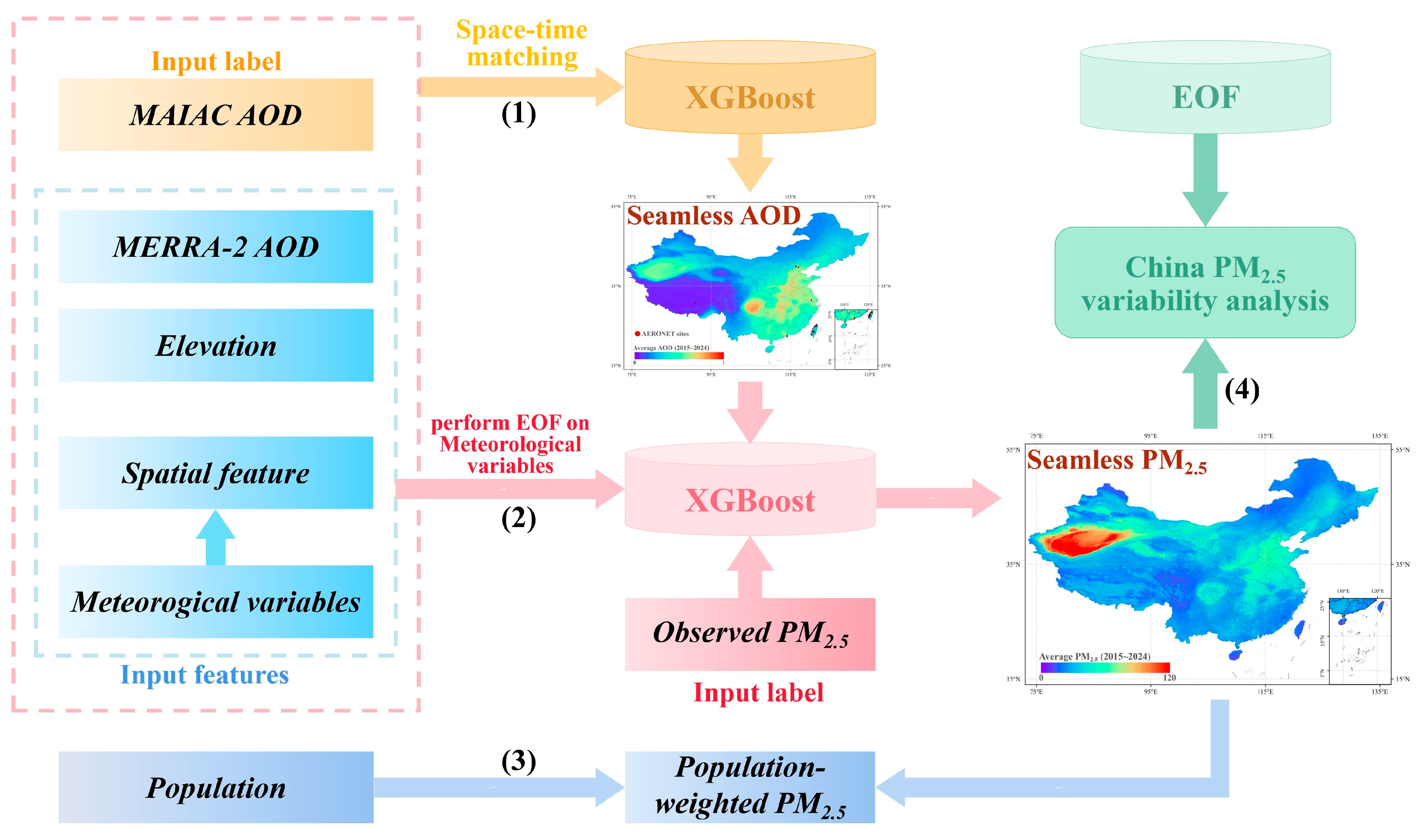
In this study, the China region is divided into 6000 × 7000 grids, spanning from 0° to 60°N and 70°E to 140°E, with a spatial resolution of 0.01° per grid cell. The elevation, meteorological data, and reanalysis AOD data are all resampled to this fine resolution using the nearest-neighbor interpolation technique. For AOD reconstruction validation, we utilize AERONET AOD data within a 10 × 10 grid (0.1° × 0.1°) to calculate and compare the average AOD values. Additionally, our study involves organizing and integrating hourly datasets, such as meteorological variables and MERRA-2 AOD, into daily aggregates. It is achieved using a simple daily averaging method, where the mean values of each variable over a 24-h period are computed based on Beijing Time. We also calculate the annual averages for each meteorological variable, remove the longitude and latitude from our input features [51], and import these yearly averages to better capture the spatial relationships and reduce spatial discontinuity among training samples. Additionally, for the calculation of daily surface station PM_2.5 averages, we only consider days with more than 16 h of recorded observations.

2.3. Methodology

Generally, a novel XGBoost-based two-step PM_2.5 estimation model is established, combined with a spatio-temporal decomposition method, and then the same decomposition method is applied for variability analysis, and population-weighted PM_2.5 is calculated for exposure risk assessment. Its framework can be divided into 4 parts, which was shown in Figure 2. Firstly, the XGBoost algorithm is employed to fill daily MAIAC AOD gaps by integrating multiple input features such as MERRA-2 AOD and meteorological variables. Secondly, the XGBoost algorithm is applied to estimate daily seamless PM_2.5 by integrating input variables similar to the gap-filling of MAIAC AOD, with EOF decomposition applied to meteorological variables to enhance the accuracy of PM_2.5 estimation. Thirdly, we calculate the population-weighted PM_2.5 trend to provide a more comprehensive assessment of the impact of China’s environmental policies. Lastly, EOF decomposition is used to analyze long-term trends and anomalies for PM_2.5 in China.

2.3.1. AOD Reconstruction Model

With the help of the machine learning algorithm XGBoost, DEM, spatial features, meteorological fields, and seamless MERRA-2 AOD are utilized as input features, and MAIAC AOD is defined as the learning target to fill the MAIAC AOD gaps. The formulation of the AOD reconstruction model is as follows.

$$AO{D}_{Satellite}=f(DEM,Spatia{l}_{mete},METE,AO{D}_{MERRA-2})$$

(2)

where AOD_Satellite represents the MAIAC AOD, DEM represents elevation data, Spatial_mete is the mean values of each meteorological variable (representing spatial proximity), METE denotes meteorological variables, AOD_MERRA-2 refers to reanalysis MERRA-2 AOD, and f is the machine learning algorithm XGBoost. Note that both 10-year averages (Spatial feature in Figure 2, average of meteorological variables in 2015–2024) and the mean values over a 24-h period (Meteorological variables in Figure 2) of each meteorological variable are computed before they are chosen as features of XGBoost. We defined num_boost_round, objective, tree_method, device, eval_metric, learning_rate, max_depth, and booster specifically, keeping other hyperparameters at their default values. Detailed information about these hyperparameters is listed in

Table 1. Information about hyperparameters defined in XGBoost model.

Hyperparameters	Value	Explanation
num_boost_round	500	Number of boosting iterations, equal to trees to build, as each iteration will build a new tree.
objective	reg:squarederror	Loss function, squarederror means squared error is a loss function and needs to be minimized.
tree_method	hist	Tree construction method, here we choose histogram-based splitting for its high speed.
device	cuda	Uses NVIDIA GPU acceleration via CUDA
eval_metric	rmse	Evaluation metric, Root Mean Squared Error, is chosen here (for validation).
learning_rate	0.23	Shrinkage factor, controls step size in updates (higher = faster convergence).
max_depth	15	Maximum tree depth, controls complexity of model (higher = deeper interactions).
booster	gbtree	The type of base learner, we choose gradient-boosted decision trees.

.

2.3.2. PM_2.5 Estimation Model

The previous PM_2.5 estimation model uses the DEM, spatial features, meteorological variables, and AOD as input features, surface station PM_2.5 as the learning target, and can be expressed as follows.

$${\mathrm{PM}}_{2.5}=f(DEM,Spatia{l}_{mete},METE,AOD)$$

(3)

where PM_2.5 represents the MAIAC AOD, DEM represents elevation data, Spatial_mete is the mean values of each meteorological variable (representing spatial proximity), METE denotes meteorological variables, AOD refers to the filled MAIAC AOD, and f is the machine learning algorithm XGBoost. In this study, we performed the EOF decomposition on the meteorological variables, to introduce the whole meteorological field information for improving the estimation accuracy. The formulation of the proposed PM_2.5 model is as follows.

$${\mathrm{PM}}_{2.5}=f(DEM,Spatia{l}_{mete},MET{E}_{eof},METE,AOD)$$

(4)

where METE_eof denotes meteorological variables after EOF decomposition. We select the first 20 combinations (the total variance larger than 95%) of spatial modes and time coefficients to represent meteorological field information.

2.3.3. Empirical Orthogonal Function Analysis

EOF (Empirical Orthogonal Function) decomposition is a statistical technique used to analyze the spatial structure of multivariate data [52,53]. Similar to PCA (Principal Component Analysis), EOF decomposition fundamentally relies on calculating the eigenvalues and eigenvectors of the input dataset. By selecting a subset of eigenvectors as the new orthogonal feature space, they both aim to retain the maximum possible variance from the original dataset while eliminating redundant dimensions such as noise. However, PCA and EOF decomposition differ in implementation and application. To clarify the differences in mathematical progress, we assume a spatiotemporal dataset organized as a matrix X_m×n (with m temporal samples and n spatial grid points) and separately apply PCA and EOF decomposition to it. For PCA, temporal means are subtracted first to create an anomaly matrix X′, followed by calculating the covariance matrix C_n×n as follows, where ${\mathrm{X}}^T$ means the matrix transpose of X.

$$C={\displaystyle \frac{1}{m-1}}{X^{\prime T}X}^{\prime }$$

(5)

Finally, eigen decomposition is conducted on the covariance matrix C_n×n as follows, where Λ = diag(λ₁, …, λ_n) contains eigenvalues (λ₁ ≥ … ≥ λ_n), and columns of V are eigenvectors defining principle directions. An eigenvalue is a quantitative description of the variance that a certain eigenvector could explain, whose larger value can denote a better ability to explain the variance of the matrix X_m×n.

$$C=V{\mathsf{\Lambda }V}^T$$

(6)

Projection to all eigenvectors is simultaneously calculated and labeled as a corresponding column of PC (Principle Component) as follows.

$$PC=XV$$

(7)

On the other hand, EOF decomposition directly conducts SVD (Singular Value Decomposition) on the anomaly matrix X’ as follows, where U, $\mathsf{\Sigma }$, and V denote left singular vectors (denotes temporal evolution), a diagonal matrix of singular values (σ₁ ≥ σ₂ ≥ … ≥ σ_r, r = rank(X)), and right singular vectors (denotes spatial patterns) separately.

$$X^{\prime }=U\mathsf{\Sigma }V$$

(8)

Then, singular values can be converted to eigenvalues described in PCA as follows, and the selection criteria are identical to those in PCA.

$${\lambda }_i={\displaystyle \frac{{\sigma }_i^2}{m-1}}$$

(9)

Finally, the spatial mode (Mode) corresponding to singular value σ_i is the i-th column of V, and the principle component (PC) is the projection to the spatial mode and can be calculated as follows, where u_i is the i-th column of U.

$${PC}_i=u_i{\sigma }_i$$

(10)

The signal of value in Mode multiplied by PC shows the trend. Areas with positive multiplied values represent an increase in the multivariate data, while areas with negative values indicate the opposite. PC represents the contribution of spatial patterns to multivariate data, considering its signal and absolute value. Considering the dominant role of seasonal trends (high-frequency components) in the variability of multivariate data, it is essential to remove seasonal cycles by subtracting temporal means for studies aiming to explore long-term trends, which is called de-climatization. This ensures that the results of EOF better capture long-term trends and non-seasonal changes.

In this study, EOF decomposition, implemented using the ‘eofs’ package in Python 3.12.4, is employed to enhance the performance of PM_2.5 estimation models and to analyze the spatio-temporal variation trends of PM_2.5 in China.

2.3.4. Population-Weighted PM_2.5 Calculation

Population-weighted PM_2.5 is an indicator used to assess the actual exposure of populations to air pollution [54]. Compared to a simple regional average of PM_2.5, it significantly improves the representation of health burden at the scale of the population level. Due to the spatial heterogeneity of PM_2.5 concentrations and population distribution, simple PM_2.5 averages may fail to capture the true population exposure levels. Hence, using population-weighted PM_2.5 offers a more reliable assessment of the potential health risks associated with air pollution. The formulation of population-weighted PM_2.5 is as follows.

$$Population-weighted {PM}_{2.5}={\displaystyle \frac{{\sum }_{i=1}^{n}P{M}_{2.5}^i\ast Po{p}^i}{{\sum }_{i=1}^{n}Po{p}^i}}$$

(11)

where ${PM}_{2.5}^i$ represents the PM_2.5 concentration at grid i, $Po{p}^i$ represents the population at grid i.

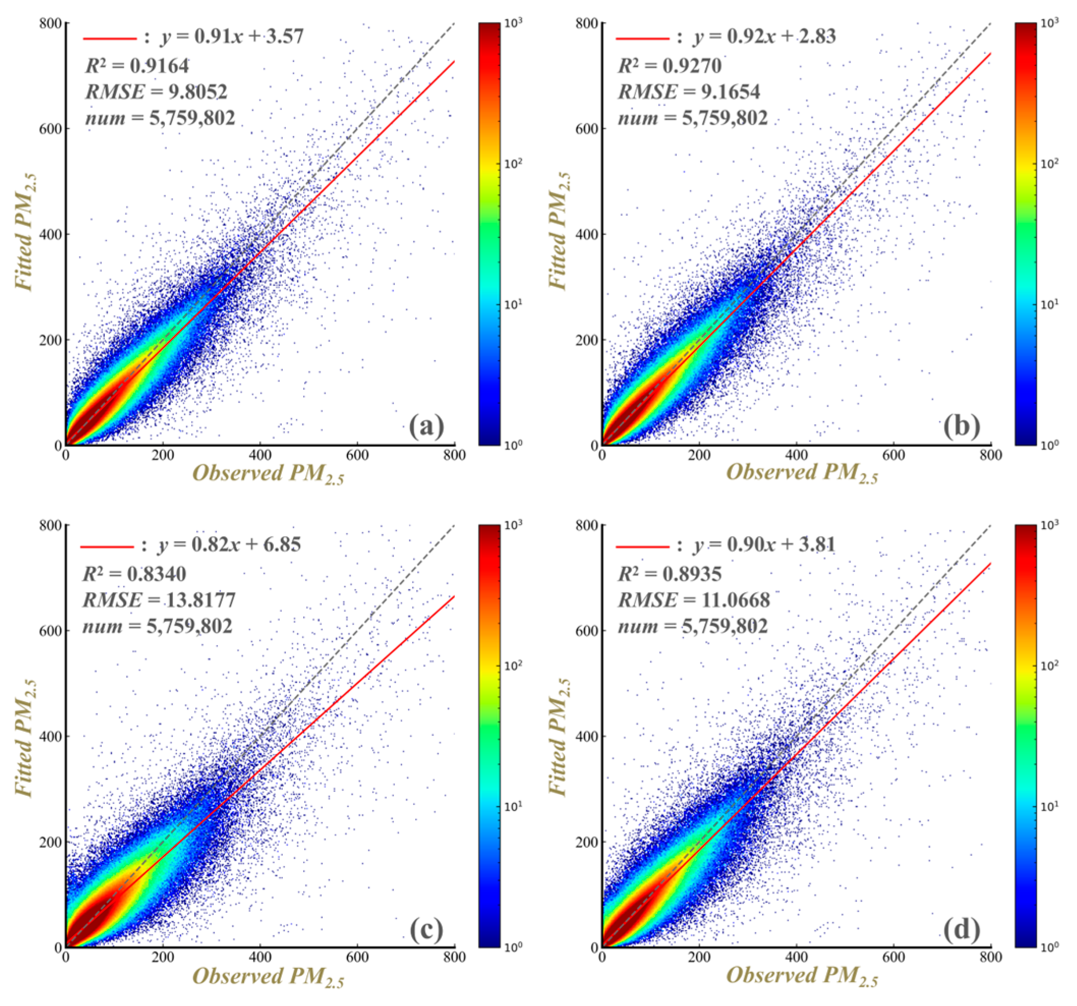
2.3.5. Model Performance Evaluation

In this study, the 10-fold sample/spatial CV (cross-validation) approach will be implemented to evaluate the accuracy of the PM_2.5 estimation model. Specifically, the CV process was repeated ten times, with each iteration 10% of the samples or sites systematically withheld as an independent test set, while the remaining 90% served as training data. The performance of the AOD reconstruction and PM_2.5 estimation models was quantitatively assessed using the coefficient of determination (R²) as well as the root mean square error (RMSE) metrics. The formulations are as follows.

$$R^2=1-{{\displaystyle {\sum }_{i=1}^n(x_i-y_i)}}^2/{{\displaystyle {\sum }_{i=1}^n(x_i-\overline{x})}}^2$$

(12)

$$RMSE=\sqrt{{\displaystyle \frac{1}{n}}{\displaystyle {\sum }_{i=1}^n{(x_i-y_i)}^2}}$$

(13)

where n symbolizes the total number of truth values, x_i denotes the truth value of the ith PM_2.5 in situ measurement, y_i represents the predicted PM_2.5 value of the ith record by the model, and $\overline{x}$ represents the mean of all truth values of PM_2.5.

3. Results

3.1. AOD Reconstruction

Figure 3 illustrates the spatial distribution of average AOD across China from 2015 to 2024, along with a comparison to AERONET AOD. To ensure the high quality of AERONET observations, level 2.0 AERONET AOD data that falls between 1 January 2015 and 31 December 2024 is selected. However, the abundance of level 2.0 AERONET AOD data makes it hard to choose AERONET sites with level 2.0 data. Only 21 sites are selected for validating gap-filled AOD, are labeled by the red-filled points in Figure 3a, and are listed in

Table 2. Information of AERONET sites with level 2.0 AOD data in 2015–2024. Note that the boundary month in “Level 2.0 period” also has level 2.0 AOD data.

Site	Altitude(m)	Latitude (°)	Longitude (°)	Level 2.0 Period
Kashi	1298	39.504	75.930	2019.03–2019.04
NAM_CO	4737	30.773	90.962	2015.01–2017.11 2020.07–2024.06
QOMS_CAS	4288	28.365	86.948	2015.01–2019.08 2021.08–2022.06
Hong_Kong_Sheung	37	22.483	114.117	2015.04–2022.07
Hong_Kong_PolyU	12	22.303	114.180	2015.01–2019.01 2020.05–2023.06
Chen-Kung_Univ	18	22.993	120.205	2015.01–2023.08
Xitun	91	24.162	120.617	2018.01–2024.04
Douliu	60	23.712	120.545	2015.01–2018.01 2022.01–2024.02
Kaohsiung	15	22.676	120.292	2018.01–2024.11
Alishan	2416	23.508	120.813	2016.04–2016.04
Lulin	2868	23.469	120.874	2015.01–2024.12
Chiayi	62	23.496	120.496	2015.01–2018.04
TASA_Taiwan	99	24.784	121.001	2018.01–2024.06
Banqiao	16	24.998	121.4425	2017.06–2017.09
Taipei_CWB	26	25.015	121.539	2015.01–2023.01
Bamboo	1050	25.187	121.535	2016.11–2017.03
Fuguei_Cape	50	25.298	121.538	2015.10–2015.11
Taihu	16	31.421	120.215	2015.10–2016.08
XiangHe	15	39.754	116.962	2015.01–2017.05 2019.05–2022.02
Beijing	58	39.977	116.381	2015.01–2019.03
Beijing-CAMS	59	39.933	116.317	2015.01–2024.01 2024.09–2024.10

with their detailed information. As depicted in Figure 3a, high AOD values are predominantly concentrated in the North China Plain and industrialized regions, whereas lower values are observed in the mountainous and plateau areas of the west and south, such as the Tibetan Plateau. The scatter plot in Figure 3b demonstrates the linear relationship between the reconstructed AOD and AERONET AOD, yielding an R² of 0.67 and an RMSE of 0.2678. Overall, the spatial distribution of the reconstructed AOD is reasonable, and the validation results confirm its suitability for PM_2.5 estimation.

3.2. PM_2.5 Estimation

Figure 4 compares the performance of two PM_2.5 estimation models: the traditional model and the model with EOF decomposition. In this paper, we choose XGBoost as our baseline model considering its ability to parallel tree construction, its unique design of the objective function, and its precise expression of the loss function. All of those advantages enable high efficiency as well as satisfying model accuracy when XGBoost is applied to retrieve daily PM_2.5. Figure 4a,c illustrate the performance of the traditional model in the sample/spatial CV, respectively. In Figure 4a, the R² is 0.9164, with an RMSE of 9.8052, while Figure 4c shows an R² of 0.8340 and an RMSE of 13.3177. Figure 4b,d present the performance of the model with EOF decomposition, a statistical method used to extract key features from multivariate datasets, allowing for the incorporation of whole meteorological field information. In Figure 4b, the model achieves an R² of 0.9270 and an RMSE of 9.1654, while in Figure 4d, it attains an R² of 0.8935 with an RMSE of 11.0668. The results indicate that the model enhanced with EOF decomposition outperforms the traditional model in both sample CV and spatial CV. In particular, it demonstrates higher R² (ΔR² = 0.0595) and lower RMSE (ΔRMSE = −2.2509) in spatial CV, and such improvements are statistically significant (p-value < 4 × 10⁻⁹ for CV-R² improvement and p-value < 2.3 × 10⁻¹⁰ for CV-RMSE improvement). These findings confirm that incorporating EOF decomposition can significantly enhance the accuracy of PM_2.5 concentration, validating its applicability in optimizing environmental modeling.

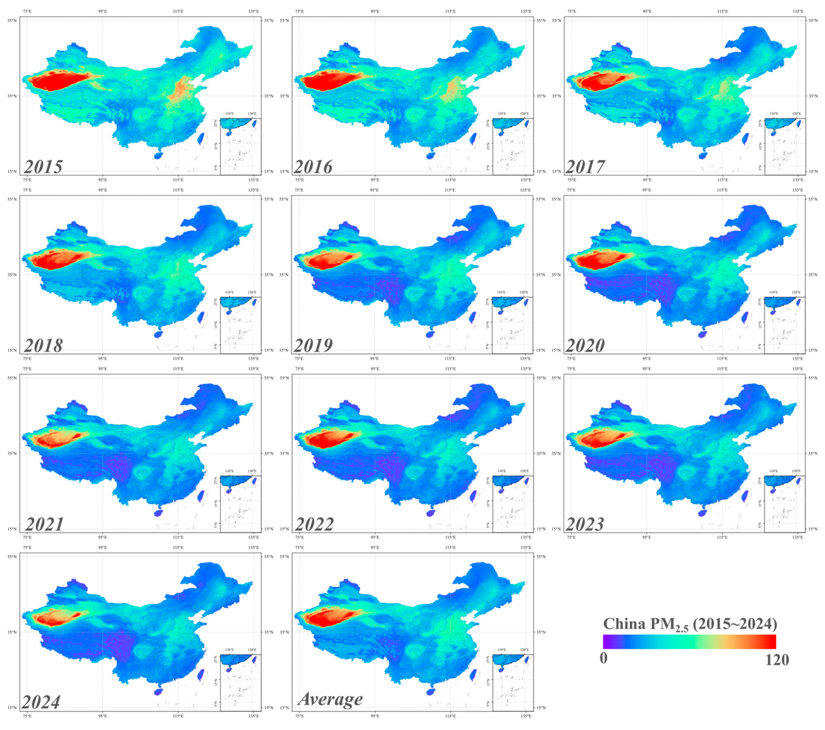
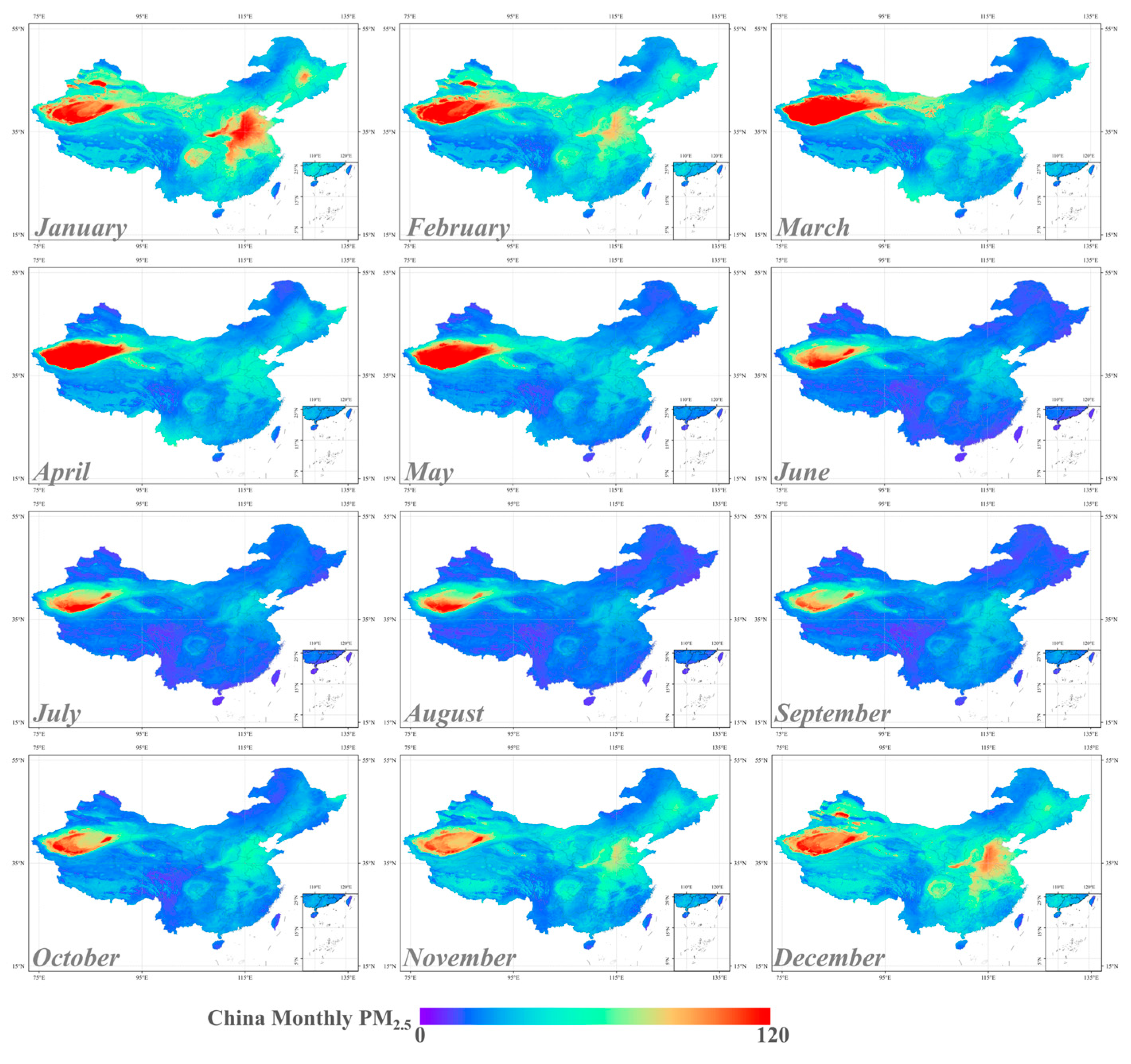
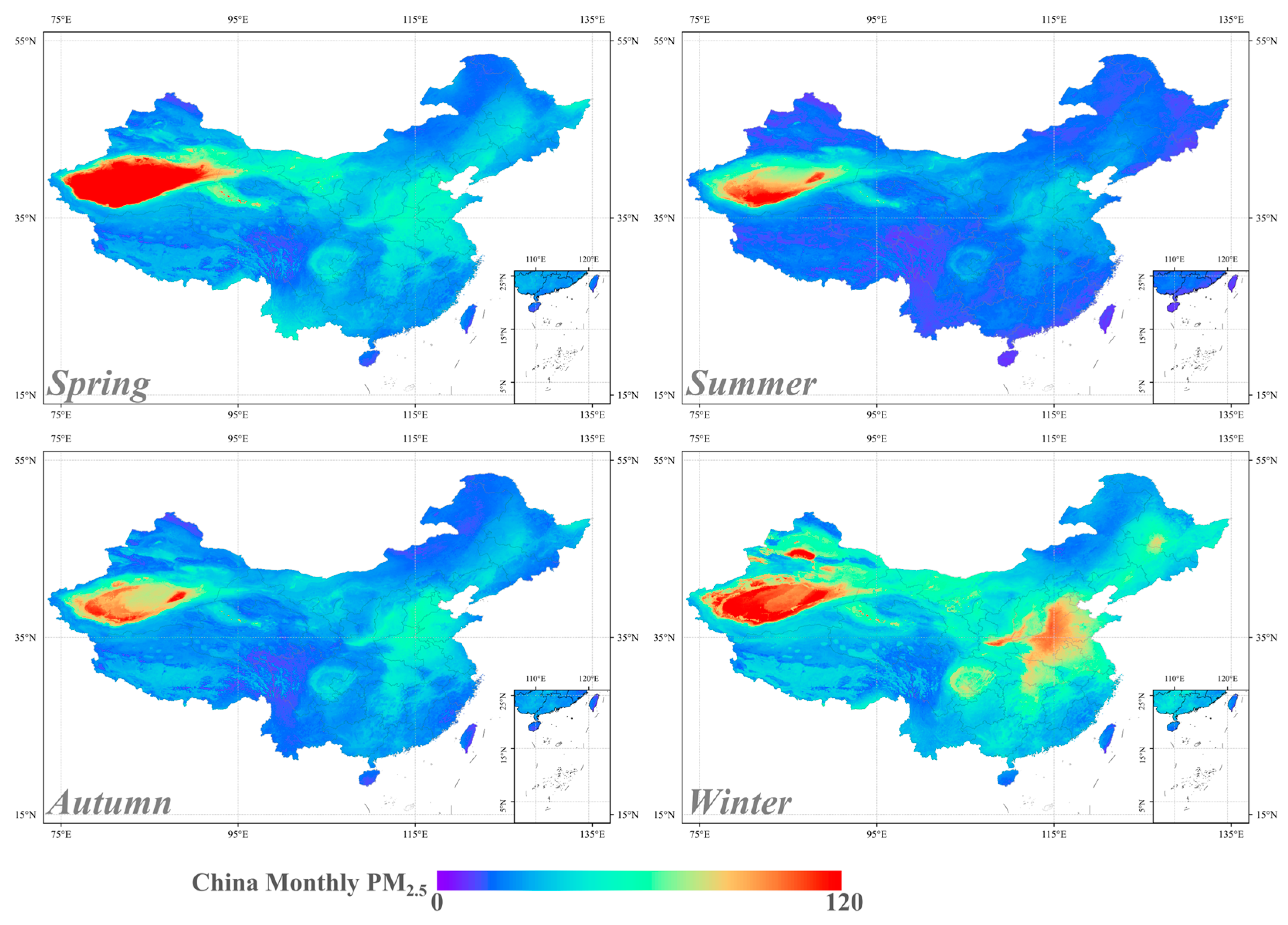
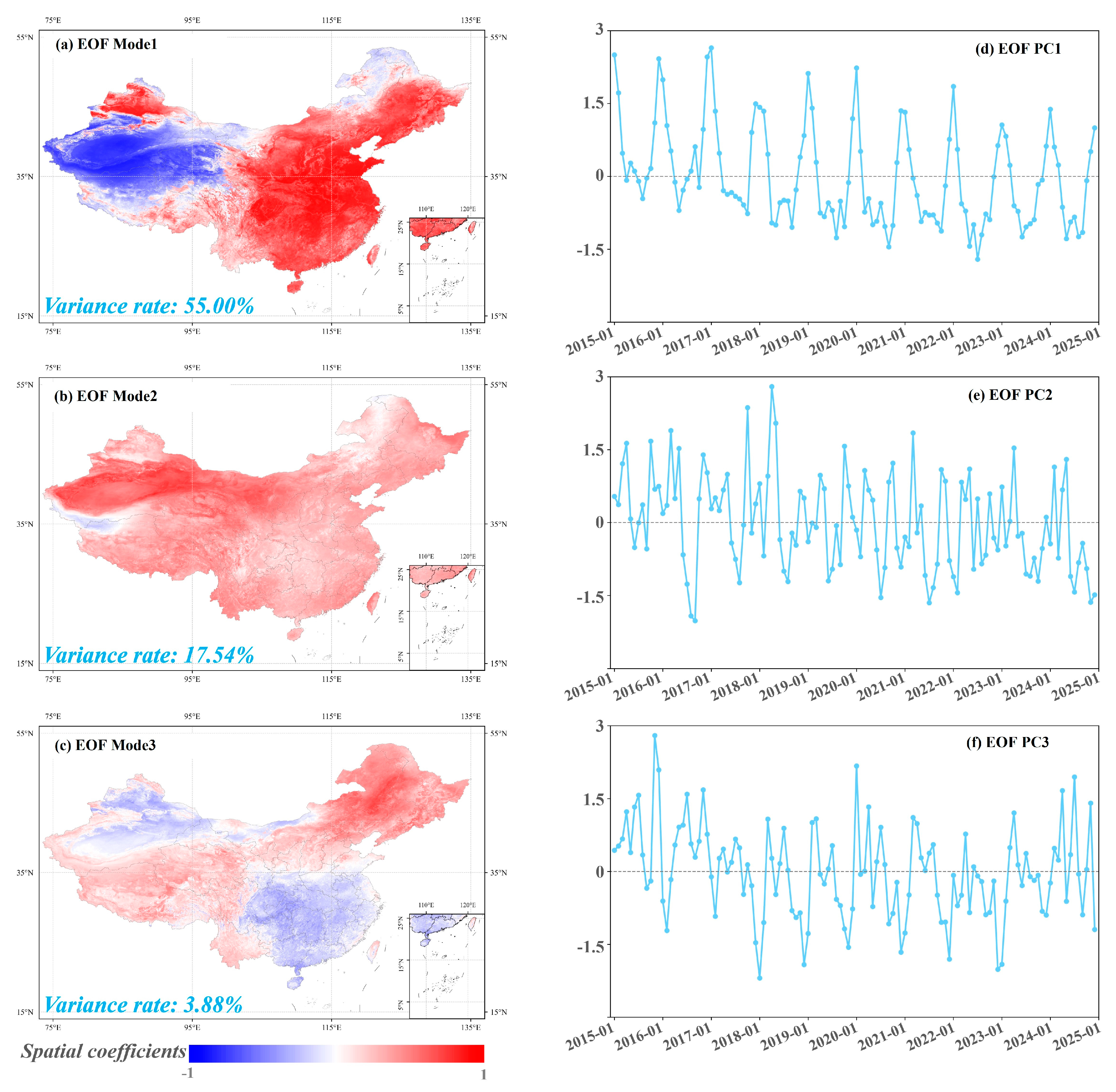
3.3. Spatio-Temporal Distribution of China PM_2.5

Figure 5 depicts the geospatial patterns of mean annual PM_2.5 concentrations (μg/m³) across China from 2015 to 2024. The results reveal that pollution levels are notably high in the North China Plain, a region marked by intensive industrial activity (coal-fired power generation, steel production), high population density (caused by megacity clusters), and heavy traffic. In contrast, the pollution levels in the Xinjiang desert region have remained consistently high throughout the observation period, showing little variation. Its high pollution levels are primarily attributed to the frequent occurrence of dust storms in the Taklimakan Desert. The decreasing spatial extent of highly polluted areas is strongly associated with the expansion of afforestation efforts in the region, which effectively mitigate emission sources of dust storms. Notably, the PM_2.5 concentrations in the eastern coastal areas have gradually declined over time, likely reflecting the effectiveness of environmental policies and industrial restructuring. However, slight heterogeneity exists in the temporal trends of different regions apart from the gradually declining trend. For example, in Tibetan Plateau, PM_2.5 showed an overall decline from 2015 to 2018, followed by minimal fluctuations post-2019; in Taklimakan Desert, PM_2.5 concentrations far below the mean PM_2.5 level of 2015–2024 occurred in 2021 and 2024, while other years aligned with long-term averages; in North China Plain, Sichuan Basin and Northeast China, steady decreases of PM_2.5 annual mean occurred from 2015 to 2020, followed by fluctuations after 2021. This inter-regional heterogeneity in temporal variation patterns motivated our choice of retaining both annual mean PM_2.5 concentrations and the mean PM_2.5 level across 2015–2024, enhancing the interpretability of annual dynamics.

Figure 6 and Figure 7 illustrate the monthly and seasonal distribution of PM_2.5 across China. Here, we adopt the same seasonal clarification strategy as in meteorology, categorizing a year into four seasons: March to May is considered spring of a year, June to August is summer, September to November is autumn, and December, together with January and February of the following year, is winter. Notably, PM_2.5 concentrations are significantly higher in the North China Plain during winter and early spring (January, February, March, and December), whose peak concentrations are witnessed in January. This is primarily attributed to increased heating demand during the cold season, as well as stagnant meteorological fields-extremely lower wind speeds than ordinary conditions, and persistent temperature inversions (<2 °C/100 m lapse rates), which suppress vertical dispersion and lead to pollutant accumulation. In contrast, PM_2.5 levels in desert regions like Xinjiang show a noticeable decline in December and January. This may be attributed to higher wind speeds during this period, which facilitates pollutant dispersion and reduces surface accumulation. The distinct seasonal variations highlight the sensitivity of different regions to meteorological conditions and human activities. To achieve precise identification of high/low PM_2.5 periods using monthly averages and better assessment of intra-annual or intra-seasonal change rates, we retained both monthly and seasonal averages. For example, PM_2.5 in the North China Plain exhibits a “rise-then-fall” pattern in winter, which is detectable via monthly mean but obscured by seasonal averaging; the monthly average of PM_2.5 in the North China Plain during summer exhibits minimal deviation from seasonal averages, which enables seasonal average to serve as a robust indicator of overall stability in PM_2.5 levels and aids in detecting subtle concentration changes. The former proves the effectiveness of the monthly average in capturing intra-seasonal change, and the latter proves the effectiveness of detecting subtle concentration changes within a season by coupling monthly and seasonal PM_2.5 levels.

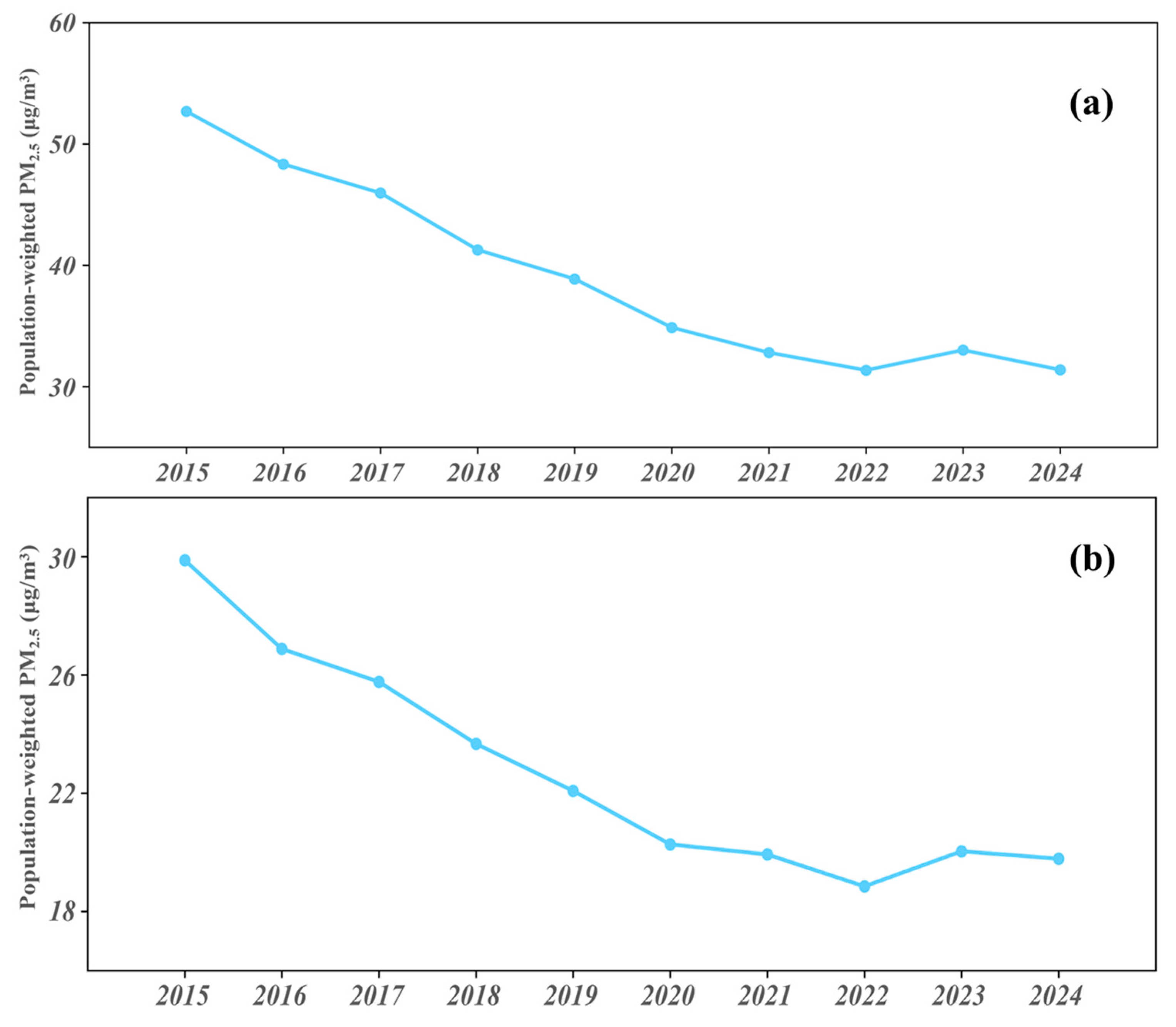
3.4. Population-Weighted PM_2.5 Concentration Trends

Figure 8 illustrates the trend of population-weighted PM_2.5 after province-averaged (Figure 8a) and the nationally aggregated population-weighted PM_2.5 concentrations (Figure 8b) in China from 2015 to 2024, calculated based on annual average PM_2.5 levels and LandScan population distribution data. The results indicate an overall declining trend in population-weighted PM_2.5 concentrations. Starting at approximately 30 µg/m³ in 2015, concentrations gradually decreased each year, reaching around 19 µg/m³ by 2020. Although slight fluctuations were observed thereafter, the overall levels remained relatively low. This trend likely reflects the effectiveness of China’s efforts to mitigate air pollution, including strengthening industrial pollution control measures and promoting the adoption of clean energy. However, the stabilization with fluctuations was observed between 2020 and 2024. Some possible reasons for the fluctuation are the government’s supporting policies for high-tech industries such as new energy vehicles and the rapid industrial transformation accelerated by the COVID-19 (Coronavirus disease) pandemic. The above analysis suggests that continued implementation of strong environmental policies is necessary to further reduce pollution levels and meet WHO (World Health Organization) air quality standards (5 µg/m³).

In addition, similar studies showed a descending trend in population-weighted PM_2.5, despite the differences in spatial resolution of the PM_2.5 dataset. For example, Cohen et al. found population-weighted PM_2.5 is 58.4 µg/m³ in 2015 [55], Zhang et al. estimated that population-weighted PM_2.5 reduced to 42.0 µg/m³ (95% CI (Confidence Interval): 35.7–48.6 µg/m³) in 2017 using WRF-CMAQ (Weather Research and Forecasting-Community Multiscale Air Quality) simulation [56], and the estimation of population-weighted PM_2.5 by Xiao et al. is almost the same as our result [57]. The rigorous difference shall be attributed to the difference in spatial resolution of the PM_2.5 dataset firstly (Cohen et al. and Xiao et al. use PM_2.5 at 0.1° resolution), and the difference in estimating method shall also be taken into consideration (Zhang et al) [56]. use WRF-CMAQ simulation and assimilated emission inventory into the model, while our model simply considers PM_2.5 observation). This overall consistency indicates the robustness of our PM_2.5 retrieval algorithm and the population-weighted PM_2.5 estimation. On the other hand, the sharp decrease between subplots a and b of Figure 8 shows that provinces with higher PWE tend to have more population, which highlights the health effects of controlling PM_2.5 concentration in highly polluted provinces.

4. Discussion

Figure 9 presents the first three modes derived from the EOF decomposition of the monthly average PM_2.5 dataset for China from 2015 to 2024 (without de-climatization). We first selected the top three largest singular values (SVs) by magnitude after SVD was applied in EOF decomposition. Then, we preserve the first 3 columns of V corresponding to the top 3 largest SVs, as their ordering is intrinsically linked. Finally, the projection of the original time series dataset onto the first three columns of the extracted V matrix is calculated, which captures the temporal trends and is shown as EOF PC in Figure 9. Simultaneously, the first three columns of the V matrix are reshaped into a matrix matching the original dataset’s dimensions and are shown as the EOF Model in Figure 9. These reshaped columns of the V matrix reveal the primary spatio-temporal variation patterns of PM_2.5. The first mode, which explains 55% of the variance, primarily covers the heavy industrial regions of eastern China and exhibits seasonal fluctuations. The spatial pattern of the first mode is likely influenced by the industrial scale as well as population. The first mode contributes the most to PM_2.5 in winter and the least in summer, which is likely influenced by winter heating and summer rainfall. The second mode, accounting for 17.54% of the variance, represents a nationwide pattern, with a long-term downward trend that may reflect the effectiveness of environmental policies. The third mode, explaining 3.88% of the variance, highlights the contrast between northern and southern China. Its complex fluctuations may be associated with regional climate conditions and policy differences. These modes collectively capture the influence of industrial activity, seasonal climatic variations, and environmental regulations on PM_2.5 concentrations. Among them, the seasonal fluctuation is the most obvious temporal trend, while the distinction in PM_2.5 between the east and the west contributes most to the spatial variation in the China monthly average PM_2.5 dataset.

Figure 10 presents the results of EOF decomposition applied to China’s monthly average PM_2.5 dataset from 2015 to 2024 after de-climatization, highlighting anomalous PM_2.5 concentration signals overshadowed by seasonal fluctuations. The first mode, which explains 32.44% of the variance, reveals significant differences in PM_2.5 concentrations between eastern and western China, similar to Figure 9. Apart from that, eastern China bears a higher spatial coefficient than that of southern and southwestern China. Its associated time series suggests seasonal fluctuations, and the variation in spatial coefficients greater than 0 may be influenced by seasonal industrial activities and increased heating demand. The second mode, accounting for 23.09% of the variance, is similar to the corresponding mode in Figure 9 and exhibits a widespread variation pattern. Its temporal fluctuations may reflect the impact of climate change or air quality policies. The third mode, explaining 5.44% of the variance, highlights a contrast between northern and southern China. The increase in PM_2.5 in winter is mainly attributed to the emissions in northern China, while such an increase is mainly attributed to the contribution of southern and central China. The shift in areas contributing to the increase of PM_2.5 in different seasons indicates the influence of regional policy implementation and meteorological conditions. These modes suggest that seasonal variations, regional disparities, and relevant policies and activities are the primary factors shaping PM_2.5 distribution. In a word, EOF decomposition without de-climatization can reveal the overall trend of PM_2.5 levels in China, while EOF after de-climatization can highlight the inter-regional disparities in PM_2.5 and elucidate its spatial distribution pattern.

5. Conclusions

This study underscores the effectiveness of integrating advanced machine learning techniques with whole meteorological field information to enhance PM_2.5 estimation accuracy across diverse geographical and climatic conditions in China. The combination of XGBoost and EOF decomposition has proven particularly effective (site-based 10-fold CV R² and RMSE change (ΔR²/ΔRMSE) = 0.0595/−2.2509) in capturing the complex spatio-temporal dynamics of PM_2.5, which are influenced by both anthropogenic activities and natural meteorological variations. This enhanced modeling approach not only demonstrates exceptional accuracy and reliability but also provides crucial insights for air quality management and health risk assessment, particularly in regions with high levels of industrial pollution and urbanization.

References

1. Pui, D.Y.; Chen, S.C.; Zuo, Z. Pm2.5 in China: Measurements, Sources, Visibility and Health Effects, and Mitigation. Particuology 2014, 13, 1–26. [Google Scholar] [CrossRef]
2. Geng, G.; Zheng, Y.; Zhang, Q.; Xue, T.; Zhao, H.; Tong, D.; Zheng, B.; Li, M.; Liu, F.; Hong, C.; et al. Drivers of Pm2.5 Air Pollution Deaths in China 2002–2017. Nat. Geosci. 2021, 14, 645–650. [Google Scholar] [CrossRef]
3. Song, C.; He, J.; Wu, L.; Jin, T.; Chen, X.; Li, R.; Ren, P.; Zhang, L.; Mao, H. Health Burden Attributable to Ambient Pm2.5 in China. Environ. Pollut. 2017, 223, 575–586. [Google Scholar] [CrossRef]
4. Wang, F.; Chen, T.; Chang, Q.; Kao, Y.-W.; Li, J.; Chen, M.; Li, Y.; Shia, B.-C. Respiratory Diseases Are Positively Associated with Pm2.5 Concentrations in Different Areas of Taiwan. PLoS ONE 2021, 16, e0249694. [Google Scholar] [CrossRef] [PubMed]
5. Hayes, R.B.; Lim, C.; Zhang, Y.; Cromar, K.; Shao, Y.; Reynolds, H.R.; Silverman, D.T.; Jones, R.R.; Park, Y.; Jerrett, M.; et al. Pm2.5 Air Pollution and Cause-Specific Cardiovascular Disease Mortality. Int. J. Epidemiol. 2020, 49, 25–35. [Google Scholar] [CrossRef]
6. State Council of the People’s Republic of China; Central People’s Government of the State Republic of China. Air Pollution Prevention and Control Action Plan; State Council of the People’s Republic of China, Central People’s Government of the State Republic of China: Beijing, China, 2013. [Google Scholar]
7. Guo, B.; Wu, H.; Pei, L.; Zhu, X.; Zhang, D.; Wang, Y.; Luo, P. Study on the Spatiotemporal Dynamic of Ground-Level Ozone Concentrations on Multiple Scales across China during the Blue Sky Protection Campaign. Environ. Int. 2022, 170, 107606. [Google Scholar] [CrossRef] [PubMed]
8. Shen, Y.; Ahlers, A.L. Blue Sky Fabrication in China: Science-Policy Integration in Air Pollution Regulation Campaigns for Mega-Events. Environ. Sci. Policy 2019, 94, 135–142. [Google Scholar] [CrossRef]
9. Shen, Y.; Zhang, X. Blue Sky Protection Campaign: Assessing the Role of Digital Technology in Reducing Air Pollution. Systems 2024, 12, 55. [Google Scholar] [CrossRef]
10. Yu, Y.; Dai, C.; Wei, Y.; Ren, H.; Zhou, J. Air Pollution Prevention and Control Action Plan Substantially Reduced Pm2.5 Concentration in China. Energy Econ. 2022, 113, 106206. [Google Scholar] [CrossRef]
11. Li, T.; Shen, H.; Zeng, C.; Yuan, Q.; Zhang, L. Point-Surface Fusion of Station Measurements and Satellite Observations for Mapping Pm2.5 Distribution in China: Methods and Assessment. Atmos. Environ. 2017, 152, 477–489. [Google Scholar] [CrossRef]
12. Kim, K.Y.; Kim, Y.S.; Roh, Y.M.; Lee, C.M.; Kim, C.N. Spatial Distribution of Particulate Matter (Pm10 and Pm2.5) in Seoul Metropolitan Subway Stations. J. Hazard. Mater. 2008, 154, 440–443. [Google Scholar] [CrossRef] [PubMed]
13. Cavaliere, A.; Carotenuto, F.; Di Gennaro, F.; Gioli, B.; Gualtieri, G.; Martelli, F.; Matese, A.; Toscano, P.; Vagnoli, C.; Zaldei, A. Development of Low-Cost Air Quality Stations for Next Generation Monitoring Networks: Calibration and Validation of Pm2.5 and Pm10 Sensors. Sensors 2018, 18, 2843. [Google Scholar] [CrossRef] [PubMed]
14. Hu, X.; Belle, J.H.; Meng, X.; Wildani, A.; Waller, L.A.; Strickland, M.J.; Liu, Y. Estimating Pm2.5 Concentrations in the Conterminous United States Using the Random Forest Approach. Environ. Sci. Technol. 2017, 51, 6936–6944. [Google Scholar] [CrossRef] [PubMed]
15. Song, W.; Jia, H.; Huang, J.; Zhang, Y. A Satellite-Based Geographically Weighted Regression Model for Regional Pm2.5 Estimation over the Pearl River Delta Region in China. Remote Sens. Environ. 2014, 154, 1–7. [Google Scholar] [CrossRef]
16. Zhang, G.; Rui, X.; Fan, Y. Critical Review of Methods to Estimate Pm2.5 Concentrations within Specified Research Region. ISPRS Int. J. Geo-Inf. 2018, 7, 368. [Google Scholar] [CrossRef]
17. Fang, X.; Zou, B.; Liu, X.; Sternberg, T.; Zhai, L. Satellite-Based Ground Pm2.5 Estimation Using Timely Structure Adaptive Modeling. Remote Sens. Environ. 2016, 186, 152–163. [Google Scholar] [CrossRef]
18. Diao, M.; Holloway, T.; Choi, S.; O’Neill, S.M.; Al-Hamdan, M.Z.; Van Donkelaar, A.; Martin, R.V.; Jin, X.; Fiore, A.M.; Henze, D.K.; et al. Methods, Availability, and Applications of Pm2.5 Exposure Estimates Derived from Ground Measurements, Satellite, and Atmospheric Models. J. Air Waste Manag. Assoc. 2019, 69, 1391–1414. [Google Scholar] [CrossRef]
19. Baker, K.R.; Foley, K.M. A Nonlinear Regression Model Estimating Single Source Concentrations of Primary and Secondarily Formed Pm2.5. Atmos. Environ. 2011, 45, 3758–3767. [Google Scholar] [CrossRef]
20. Liu, Y.; Sarnat, J.A.; Kilaru, V.; Jacob, D.J.; Koutrakis, P. Estimating Ground-Level Pm2.5 in the Eastern United States Using Satellite Remote Sensing. Environ. Sci. Technol. 2005, 39, 3269–3278. [Google Scholar] [CrossRef]
21. Hien, P.D.; Bac, V.T.; Tham, H.C.; Nhan, D.D.; Vinh, L.D. Influence of Meteorological Conditions on Pm2.5 and Pm2.5−10 Concentrations during the Monsoon Season in Hanoi, Vietnam. Atmos. Environ. 2002, 36, 3473–3484. [Google Scholar] [CrossRef]
22. Chen, L.W.A.; Watson, J.G.; Chow, J.C.; Magliano, K.L. Quantifying Pm2.5 Source Contributions for the San Joaquin Valley with Multivariate Receptor Models. Environ. Sci. Technol. 2007, 41, 2818–2826. [Google Scholar] [CrossRef] [PubMed]
23. Vallius, M.; Janssen, N.A.H.; Heinrich, J.; Hoek, G.; Ruuskanen, J.; Cyrys, J.; Van Grieken, R.; de Hartog, J.J.; Kreyling, W.G.; Pekkanen, J. Sources and Elemental Composition of Ambient Pm2.5 in Three European Cities. Sci. Total Environ. 2005, 337, 147–162. [Google Scholar] [CrossRef]
24. Zhou, Y.; Chang, F.-J.; Chang, L.-C.; Kao, I.-F.; Wang, Y.-S.; Kang, C.-C. Multi-Output Support Vector Machine for Regional Multi-Step-Ahead Pm2.5 Forecasting. Sci. Total Environ. 2019, 651, 230–240. [Google Scholar] [CrossRef]
25. Liu, Y.; Cao, G.; Zhao, N.; Mulligan, K.; Ye, X. Improve Ground-Level Pm2.5 Concentration Mapping Using a Random Forests-Based Geostatistical Approach. Environ. Pollut. 2018, 235, 272–282. [Google Scholar] [CrossRef]
26. Kow, P.-Y.; Chang, L.-C.; Lin, C.-Y.; Chou, C.C.-K.; Chang, F.-J. Deep Neural Networks for Spatiotemporal Pm2.5 Forecasts Based on Atmospheric Chemical Transport Model Output and Monitoring Data. Environ. Pollut. 2022, 306, 119348. [Google Scholar] [CrossRef] [PubMed]
27. Wang, J.; Ogawa, S. Effects of Meteorological Conditions on Pm2.5 Concentrations in Nagasaki, Japan. Int. J. Environ. Res. Public Health 2015, 12, 9089–9101. [Google Scholar] [CrossRef]
28. Xu, Y.; Xue, W.; Lei, Y.; Zhao, Y.; Cheng, S.; Ren, Z.; Huang, Q. Impact of Meteorological Conditions on Pm2.5 Pollution in China during Winter. Atmosphere 2018, 9, 429. [Google Scholar] [CrossRef]
29. Chen, Z.; Chen, D.; Zhao, C.; Kwan, M.P.; Cai, J.; Zhuang, Y.; Zhao, B.; Wang, X.; Chen, B.; Yang, J.; et al. Influence of Meteorological Conditions on Pm2.5 Concentrations across China: A Review of Methodology and Mechanism. Environ. Int. 2020, 139, 105558. [Google Scholar] [CrossRef]
30. Xu, Y.; Xue, W.; Lei, Y.; Huang, Q.; Zhao, Y.; Cheng, S.; Ren, Z.; Wang, J. Spatiotemporal Variation in the Impact of Meteorological Conditions on Pm2.5 Pollution in China from 2000 to 2017. Atmos. Environ. 2020, 223, 117215. [Google Scholar] [CrossRef]
31. Ding, Y.; Chen, Z.; Lu, W.; Wang, X. A Catboost Approach with Wavelet Decomposition to Improve Satellite-Derived High-Resolution Pm2.5 Estimates in Beijing-Tianjin-Hebei. Atmos. Environ. 2021, 249, 118212. [Google Scholar] [CrossRef]
32. Ding, Y.; Li, S.; Xing, J.; Li, X.; Ma, X.; Song, G.; Teng, M.; Yang, J.; Dong, J.; Meng, S. Retrieving Hourly Seamless Pm2.5 Concentration across China with Physically Informed Spatiotemporal Connection. Remote Sens. Environ. 2024, 301, 113901. [Google Scholar] [CrossRef]
33. Pruthi, D.; Zhu, Q.; Wang, W.; Liu, Y. Multiresolution Analysis of Hrrr Meteorological Parameters and Goes-R Aod for Hourly Pm2.5 Prediction. Environ. Sci. Technol. 2024, 58, 20040–20048. [Google Scholar] [CrossRef] [PubMed]
34. Yoo, C.; Kim, S. Eof Analysis of Surface Soil Moisture Field Variability. Adv. Water Resour. 2004, 27, 831–842. [Google Scholar] [CrossRef]
35. Ludwig, F.L.; Horel, J.; Whiteman, C.D. Using Eof Analysis to Identify Important Surface Wind Patterns in Mountain Valleys. J. Appl. Meteorol. 2004, 43, 969–983. [Google Scholar] [CrossRef]
36. Xiao-Feng, L.; Pietrafesa, L.; Shu-Fang, L.; Li-An, X. Significance Test for Empirical Orthogonal Function (Eof) Analysis of Meteorological and Oceanic Data. Chin. J. Oceanol. Limnol. 2000, 18, 10–17. [Google Scholar] [CrossRef]
37. Zhou, K.; Yang, S. Emission Reduction of China’s Steel Industry: Progress and Challenges. Renew. Sustain. Energy Rev. 2016, 61, 319–327. [Google Scholar] [CrossRef]
38. Xu, C.; Huo, X.; Hong, Y.; Yu, C.; de Jong, M.; Cheng, B. How Urban Greening Policy Affects Urban Ecological Resilience: Quasi-Natural Experimental Evidence from Three Megacity Clusters in China. J. Clean. Prod. 2024, 452, 142233. [Google Scholar] [CrossRef]
39. Lyapustin, A.; Wang, Y.; Korkin, S.; Huang, D. Modis Collection 6 Maiac Algorithm. Atmos. Meas. Tech. 2018, 11, 5741–5765. [Google Scholar] [CrossRef]
40. Lyapustin, A.; Wang, Y.; Laszlo, I.; Kahn, R.; Korkin, S.; Remer, L.; Levy, R.; Reid, J.S. Multiangle Implementation of Atmospheric Correction (Maiac): 2. Aerosol Algorithm. J. Geophys. Res. Atmos. 2011, 116. [Google Scholar] [CrossRef]
41. Lyapustin, A.I.; Wang, Y.; Laszlo, I.; Hilker, T.; Hall, F.G.; Sellers, P.J.; Tucker, C.J.; Korkin, S.V. Multi-Angle Implementation of Atmospheric Correction for Modis (Maiac): 3. Atmospheric Correction. Remote Sens. Environ. 2012, 127, 385–393. [Google Scholar] [CrossRef]
42. Gelaro, R.; McCarty, W.; Suárez, M.J.; Todling, R.; Molod, A.; Takacs, L.; Randles, C.A.; Darmenov, A.; Bosilovich, M.G.; Reichle, R.; et al. The Modern-Era Retrospective Analysis for Research and Applications, Version 2 (Merra-2). J. Clim. 2017, 30, 5419–5454. [Google Scholar] [CrossRef]
43. Buchard, V.; Randles, C.A.; Da Silva, A.M.; Darmenov, A.; Colarco, P.R.; Govindaraju, R.; Ferrare, R.; Hair, J.; Beyersdorf, A.J.; Ziemba, L.D.; et al. The Merra-2 Aerosol Reanalysis, 1980 Onward. Part Ii: Evaluation and Case Studies. J. Clim. 2017, 30, 6851–6872. [Google Scholar] [CrossRef] [PubMed]
44. Sun, E.; Xu, X.; Che, H.; Tang, Z.; Gui, K.; An, L.; Lu, C.; Shi, G. Variation in Merra-2 Aerosol Optical Depth and Absorption Aerosol Optical Depth over China from 1980 to 2017. J. Atmos. Sol.-Terr. Phys. 2019, 186, 8–19. [Google Scholar] [CrossRef]
45. Andrews, E.; Ogren, J.A.; Kinne, S.; Samset, B. Comparison of Aod, Aaod and Column Single Scattering Albedo from Aeronet Retrievals and in Situ Profiling Measurements. Atmos. Chem. Phys. 2017, 17, 6041–6072. [Google Scholar] [CrossRef]
46. Sorek-Hamer, M.; Franklin, M.; Chau, K.; Garay, M.; Kalashnikova, O. Spatiotemporal Characteristics of the Association between Aod and Pm over the California Central Valley. Remote Sens. 2020, 12, 685. [Google Scholar] [CrossRef]
47. Hersbach, H.; Bell, B.; Berrisford, P.; Hirahara, S.; Horányi, A.; Muñoz-Sabater, J.; Nicolas, J.; Peubey, C.; Radu, R.; Schepers, D.; et al. The Era5 Global Reanalysis. Q. J. R. Meteorol. Soc. 2020, 146, 1999–2049. [Google Scholar] [CrossRef]
48. Hallgren, C.; Aird, J.A.; Ivanell, S.; Körnich, H.; Vakkari, V.; Barthelmie, R.J.; Pryor, S.C.; Sahlée, E. Machine Learning Methods to Improve Spatial Predictions of Coastal Wind Speed Profiles and Low-Level Jets Using Single-Level Era5 Data. Wind Energ. Sci. 2024, 9, 821–840. [Google Scholar] [CrossRef]
49. Han, H.; Zeng, Q.; Jiao, J. Quality Assessment of Tandem-X Dems, Srtm and Aster Gdem on Selected Chinese Sites. Remote Sens. 2021, 13, 1304. [Google Scholar] [CrossRef]
50. Hanberry, B.B. Imposing Consistent Global Definitions of Urban Populations with Gridded Population Density Models: Irreconcilable Differences at the National Scale. Landsc. Urban Plan. 2022, 226, 104493. [Google Scholar] [CrossRef]
51. Ni, W.; Ding, Y.; Li, S.; Teng, M.; Yang, J. Estimation of Daily Seamless Pm2.5 Concentrations with Climate Feature in Hubei Province, China. Remote Sens. 2023, 15, 3822. [Google Scholar] [CrossRef]
52. Kim, K.Y.; Wu, Q. A Comparison Study of Eof Techniques: Analysis of Nonstationary Data with Periodic Statistics. J. Clim. 1999, 12, 185–199. [Google Scholar] [CrossRef]
53. Sauquet, E.; Krasovskaia, I.; Leblois, E. Mapping Mean Monthly Runoff Pattern Using Eof Analysis. Hydrol. Earth Syst. Sci. 2000, 4, 79–93. [Google Scholar] [CrossRef]
54. Aunan, K.; Ma, Q.; Lund, M.T.; Wang, S. Population-Weighted Exposure to Pm2.5 Pollution in China: An Integrated Approach. Environ. Int. 2018, 120, 111–120. [Google Scholar] [CrossRef] [PubMed]
55. Cohen, A.J.; Brauer, M.; Burnett, R.; Anderson, H.R.; Frostad, J.; Estep, K.; Balakrishnan, K.; Brunekreef, B.; Dandona, L.; Dandona, R.; et al. Forouzanfar. Estimates and 25-Year Trends of the Global Burden of Disease Attributable to Ambient Air Pollution: An Analysis of Data from the Global Burden of Diseases Study 2015. Lancet 2017, 389, 1907–1918. [Google Scholar] [CrossRef] [PubMed]
56. Zhang, Q.; Zheng, Y.; Tong, D.; Shao, M.; Wang, S.; Zhang, Y.; Xu, X.; Wang, J.; He, H.; Liu, W.; et al. Drivers of Improved Pm2.5 Air Quality in China from 2013 to 2017. Proc. Natl. Acad. Sci. USA 2019, 116, 24463–24469. [Google Scholar] [CrossRef]
57. Xiao, Q.; Geng, G.; Xue, T.; Liu, S.; Cai, C.; He, K.; Zhang, Q. Tracking Pm and O3 Pollution and the Related Health Burden in China 2013–2020. Environ. Sci. Technol. 2022, 56, 6922–6932. [Google Scholar] [CrossRef]
Figure 1. Map of study area showing 2025 ground PM2.5 in situ measurement sites (dark orange dots) and elevation (colorful shading, unit: meters).
Remotesensing 17 01632 g001
Figure 2. Graphical representation of this study. (1) Gap-filling of AOD (Aerosol Optical Depth, highlighted in yellow). (2) Estimating seamless PM2.5 using EOF (Empirical Orthogonal Function, highlighted in red). (3) Calculating annual population-weighted PM2.5 (highlighted in blue). (4) decompositing seamless PM2.5 (highlighted in green). Detailed information can be found in Section 2.3.
Remotesensing 17 01632 g002
Figure 3. (a) The spatial distribution of China’s average AOD during 2015–2024; (b) comparison of daily AERONET (Aerosol Robotic Network) AOD (as the ground truth) with fusion AOD. The black dotted line is a 1:1 line, defined as y = x.
Remotesensing 17 01632 g003
Figure 4. (a) The sample CV (cross-validation) of the traditional estimation model; (b) the sample CV of the proposed estimation model with EOF decomposition; (c) the spatial CV of the traditional estimation model; (d) the spatial CV of the proposed estimation model with EOF decomposition. The black dotted lines in (ad) are 1:1 lines, defined as y = x.
Remotesensing 17 01632 g004
Figure 5. The spatial distribution of China’s annual PM2.5 during 2015–2024.
Remotesensing 17 01632 g005
Figure 6. The spatial distribution of China’s monthly PM2.5 during 2015–2024.
Remotesensing 17 01632 g006
Figure 7. The spatial distribution of China’s seasonal PM2.5 during 2015–2024.
Remotesensing 17 01632 g007
Figure 8. (a) Province-averaged population-weighted PM2.5 concentration trends and (b) nationally aggregated population-weighted PM2.5 concentrations in China (2015–2024).
Remotesensing 17 01632 g008
Figure 9. The spatial distribution (ac) and time coefficients (df) of mode 1 (a,d), 2 (b,e), 3 (c,f) for China PM2.5 (perform no de-climatization).
Remotesensing 17 01632 g009
Figure 10. The spatial distribution (ac) and time coefficients (df) of mode 1 (a,d), 2 (b,e), 3 (c,f) for China PM2.5 (perform de-climatization).
Remotesensing 17 01632 g010