Article

Structural Similarity-Guided Siamese U-Net Model for Detecting Changes in Snow Water Equivalent

by
Karim Malik
1,* and
Colin Robertson
2
1
School of the Environment, University of Windsor, Windsor, ON N9B 3P4, Canada
2
Department of Geography and Environmental Studies, Wilfrid Laurier University, Waterloo, ON N2L 3C5, Canada
*
Author to whom correspondence should be addressed.
Remote Sens. 2025, 17(9), 1631; https://doi.org/10.3390/rs17091631
Submission received: 10 March 2025 / Revised: 23 April 2025 / Accepted: 29 April 2025 / Published: 4 May 2025

Abstract

:
Snow water equivalent (SWE), the amount of water generated when a snowpack melts, has been used to study the impacts of climate change on the cryosphere processes and snow cover dynamics during the winter season. In most analyses, high-temporal-resolution SWE and SD data are aggregated into monthly and yearly averages to detect and characterize changes. Aggregating snow measurements, however, can magnify the modifiable aerial unit problem, resulting in differing snow trends at different temporal resolutions. Time series analysis of gridded SWE data holds the potential to unravel the impacts of climate change and global warming on daily, weekly, and monthly changes in snow during the winter season. Consequently, this research presents a high-temporal-resolution analysis of changes in the SWE across the cold regions of Canada. A Siamese UNet (Si-UNet) was developed by modifying the model’s last layer to incorporate the structural similarity (SSIM) index. The similarity values from the SSIM index are passed to a contrastive loss function, where the optimization process maximizes SSIM index values for pairs of similar SWE images and minimizes the values for pairs of dissimilar SWE images. A comparison of different model architectures, loss functions, and similarity metrics revealed that the SSIM index and the contrastive loss improved the Si-UNet’s accuracy by 16%. Using our Si-UNet, we found that interannual SWE declined steadily from 1979 to 2018, with March being the month in which the most significant changes occurred (R2 = 0.1, p-value < 0.05). We conclude with a discussion on the implications of the findings from our study of snow dynamics and climate variables using gridded SWE data, computer vision metrics, and fully convolutional deep neural networks.

1. Introduction

Change detection in remotely sensed data is a frequently encountered problem. However, snow is a highly sensitive Earth cover category, as it is directly and indirectly affected by diverse climate variables and feedback loops, such as snow albedo feedback [1]. The Earth’s cold regions are now actively being investigated to understand global warming effects on various land-cover types, including tundra vegetation, snow, ice sheets, and permafrost landscape [2]. Snow represents an indispensable Northern Hemisphere (NH) land-cover component, especially during winter. Snow significantly influences the responses of flora, fauna, and ecosystem feedback mechanisms [2]. Melting snow produces water that feeds freshwater ecosystems and contributes to irrigation [3]. In the Arctic, snow contributes to ice-sheet thickness and influences the Arctic surface mass balance, which plays an important role in regulating the rise of the global sea level. Furthermore, the timing of snow retreat partly defines the onset of wildfire season, especially in North American countries, such as Canada. Snow parameters, such as the SWE, snow depth, snow density, and snow spatial extent, are essential sentinels of environmental change. Due to snow’s inherent sensitivity to increasing surface temperature and precipitation, these parameters have been monitored to infer the impact of climate change on the cryosphere.
The unique nature of snow sensitivity and variability poses challenges to detecting and attributing changes that are linked to snow responses to climate forcing agents [4]. Consequently, spurious changes associated with natural internal variability in snow signals are likely to be detected by less robust algorithms as false change scenarios. Despite this fundamental challenge in modelling and detecting changes in snow, there has been progress in characterizing trends in the snow water equivalent (SWE), snow depth (SD), and snow cover extent (SE) [5], as well as evaluating snow cover extent and properties [6].
One particular trend in the methods for studying snow parameters is the adoption of reference periods and the use of arithmetic averaging techniques on time series of snow observations. Additionally, most studies consider March to be the temporal window in which SWE and snow depth are at their peak. For example, March snow data have been employed to discover declining SWE trends in Eastern and Western Canada [7]. Similarly, Pulliainen et al. [5] used March GlobSnow data to quantify snow mass across the Northern Hemisphere and discovered declining trends. Raisanen [8] analyzed changes in the mean March SWE in reanalysis data. While these methods have yielded important insights into snow trends, arithmetic averaging can amplify the modifiable areal unit problem, where changes in data resolution lead to varying results. Furthermore, general atmospheric cycles, such as the Pacific/North America Oscillation, Pacific Decadal Oscillation, Arctic Oscillation, and El-Nino Southern Oscillation, can result in climate regime shifts that may not be easy to detect by studying SWE in a particular month [9,10].Therefore, analyzing snow trends in other temporal windows (January, February, March, and April) will provide a wealth of information on the evolution of the cryosphere’s response to natural climate cycles and global warming.
This study is, therefore, focused on three primary objectives: (a) to demonstrate the Siamese U-Net’s effectiveness for detecting changes in SWE; (b) to illustrate the utility of the SSIM index for comparing SWE similarity within a deep learning model architecture; and (c) to use Siamese U-Net predictions to estimate decadal changes in SWE trends. To our knowledge, this research represents the most recent modification of U-Net’s architecture to incorporate the SSIM index for high-temporal-resolution analysis of SWE trends in the Northern Hemisphere.

2. Related Work and Recent Progress

2.1. Progress in Snow Parameter Analysis

Point-based monitoring of snow depth, snow density, and SWE dominated cryosphere investigations until 1979, when the European Space Agency launched a space-borne microwave remote sensing satellite mission to collect gridded snow data [11]. Point-based measurements provide accurate estimates of snow parameters and have been utilized to validate satellite observations and reanalysis datasets. For example, the recent time series SWE developed in [12] offers potential for improved climate studies. Unfortunately, a conspicuous limitation inherent in all point-based observations is their inability to effectively represent the spatial structure (spatial configuration) exhibited by spatial patterns generated by spatial–temporal processes. Consequently, gridded data have been derived from point-based measurements to study snow trends [13]. Similarly, gridded snow data were employed to study SWE trends as well as evaluate global climate modelss [7,14]. Moreover, changes in North American snowpacks have been effectively documented using SMMR and SSM/I passive microwave instruments onboard satellites [15]. It is important to emphasize that regardless of the data capture technology or method used, snow exhibits intrinsic internal and interannual variability that may not be related to underlying climate anomalies or anthropogenic forcing agents [4,16]. Also, the uncertainties surrounding snow data-generating models, including reanalysis datasets, have been well documented. For instance, there are uncertainties associated with using an ensemble of models to estimate the SWE in North America [17]. The stability and continuity of climate data records are also important concerns. For example, data accuracy and stability trade-offs occur when using new data to improve snow estimates in reanalysis datasets [18]. However, GlobSnow’s SWE data, developed using the Finnish Meteorological Institute’s algorithm [11] and GlobSnow version 3.0, which comes with bias correction methods, have been found to closely approximate snow depth measurements derived from weather stations’ instruments [19]. Despite the challenges mentioned above, analysis of the trends in snow parameters has yielded valuable insights. For example, in the NH, the decrease in the SWE is largely attributed to decreases in snowfall and snow-on-ground rather than total precipitation [8]. More recently, it has been shown that snow storage index (i.e., the phase difference between daily precipitation and surface water inputs) has decreased in North America [20]. This decline is associated with early snowmelt and reduced winter precipitation. April SWE was also found to have declined significantly in the Western United States [21]. In a related study, the annual mean and maximum SWE were found to have declined in Eurasia between 1979 and 2004 [22]. These declines in winter snow have led to the emergence of snow-related streamflow drought regimes, as illustrated in [23].
Detecting and attributing changes in snow parameters, however, remains challenging. This is partly due to change detection algorithms’ sensitivity to noise, internal variability, seasonal patterns, and climate-forcing factors present in snow data products. Computer vision metrics and deep learning methods are crucial tools for addressing non-significant changes in spatial patterns and have shown promising potential [24]. For instance, CW-SSIM and SSIM have been shown to effectively detect daily SWE changes observed in April [25].

2.2. Siamese Models for Pattern Comparison

The Siamese model incorporates a parameter-sharing paradigm, resulting in “twin models” learning an identical function to compare a pair of data points. The origin of the Siamese network for pattern comparison can be found in [26]. The authors conceived a fully connected neural network architecture for comparing signatures to detect fraud. A convolutional Siamese network was later introduced to circumvent the limitations of fully connected networks in image comparison tasks. The model’s architecture employs a classical convolutional neural network (CNN) as the backbone model. Therefore, the pattern comparison task is executed using 1D feature vectors in the models’ last layers. However, this comes with certain limitations. Feature vectors derived from 2D feature maps in higher layers of deep learning models encode global patterns. As a result, 1D vectors lack contextual and local information that encodes spatial variability in images. Fully convolutional CNN models are potential algorithms for addressing this limitation.
U-Net, a fully convolutional CNN, was first introduced in [27]. This model excels at tasks involving medical image segmentation. Several sophisticated variants of the U-Net model have been widely applied across diverse tasks. For example, Residual U-Net uses skip connections, Dense U-Net uses dense layers, and Attention U-Net incorporates attention modules [28,29,30,31,32]. More recently, multiscale attention transformer networks have been introduced to detect change [33]. The inherent and key defining attributes of U-Net models are fully convolutional feature extraction, skip or residual connections, and an encoder–decoder module. Unlike CNNs with 1D dense layers, fully convolutional models retain spatial information that characterizes local structures in images. Skip or residual connections further ensure that the spatial information is not significantly diluted as the network propagates forward [34]. In other words, residual connections pass on spatial signals that define key image elements that otherwise would have been lost in previous layers, making them accessible to successive layers of the model.
With the encoder–decoder architecture, the model learns a mapping function that simultaneously deconstructs and reconstructs the underlying data. It is worth noting that the reconstruction pipeline can be challenging to efficiently attain without the fully convolutional architecture and skip connection module [34]. Such a learning framework has important implications for pattern recognition, change detection, and image content similarity analysis. By simultaneously learning image deconstruction and reconstruction mapping functions, the model implicitly understands both spatial processes that deteriorate images (e.g., high temperatures in the case of SWE) and those that form images (e.g., snowfall and sub-zero temperatures for SWE) at spatial scales constrained to the field of view of filters in various layers of the model. The U-Net architecture, therefore, has the potential to effectively analyze image content. For example, a Siamese network has been proven to detect change [35].

3. Materials and Methods

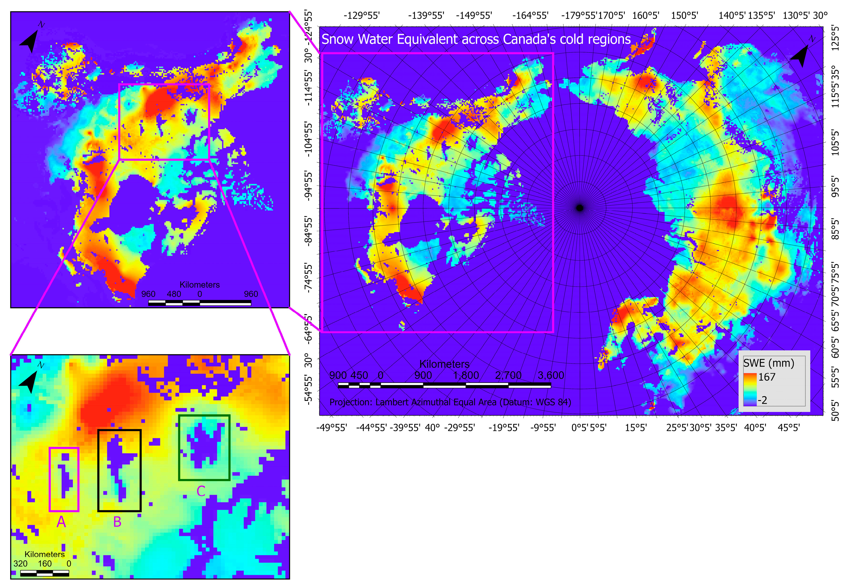
3.1. SWE Data and Study Location

Although about 65% of the Canadian land mass is covered by snow during the winter [36], it was important to select a location with a high fraction of snow cover. The data spatial extent of the study area covered the cold regions of Canada (Alberta, Yukon, and Northwest Territories), spanning latitudes from 60°N to 70°N. Snow arrives early in these regions and persists for more days than in many parts of Canada. Therefore, a high percentage of snow cover is sampled here by Earth observation instruments, making snow data accessible for deep learning-based modelling frameworks. GlobSnow’s v3.0 SWE data were derived from SWE estimates using satellite-based passive microwave technology, including Scanning Multichannel Microwave Radiometer, Special Sensor Microwave/Imager (SSM/I), and Special Sensor Microwave Imager/Sounder (SSMIS) instruments. Using ground-based snow depth measurements, Bayesian data assimilation methods, and the HUT Snow Emission model, this version circumvented most of the limitations of the earlier GlobSnow’s v2.0 SWE products, as bias-correction procedures have been implemented to account for uncertainties in SWE estimation. Further technical details pertaining to the derivation of the SWE data and their suitability for climate studies are provided in [37]. In Figure 1, we present a SWE map to illustrate the spatial distribution of SWE in Canada. It can be observed that the cold regions (shown in the pink rectangle) depict spatially varying SWE, interspersed with water bodies (lakes, rivers, and seas/oceans). Also, it is notable that the areas surrounding Lake Athabasca (A), Great Bear Lake (B), and Great Slave Lake (C) showed elevated levels of SWE.

3.2. SWE Data Processing

The GlobSnow SWE data are available as NetCDF files at GlobSnow‘s website. The SWE data were downloaded from the data repository using Python scripts to automate the process. Then, the data were re-projected and clipped to the spatial extent of the study area using the GDAL library. Although re-projecting and clipping raster data can be accomplished in software, such as ENVI 6.0 and ArcGIS Pro 3.0, we opted for GDAL to unify and automate data processing and model development in the Python programming language. GDAL, Tensorflow library, and Scikit Learn were installed using the Anaconda Package Manager with Python 3.7. All SWE data where 50% of the area had no snow were discarded from the training data. This spatial discontinuity in SWE data was common in April. Mountainous terrains and water bodies are represented using negative numbers (e.g., −1 or −2). We replaced negative values with 0 and used the StandardScaler function in Scikit Learn to scale the SWE values to a range between 0 and 1.

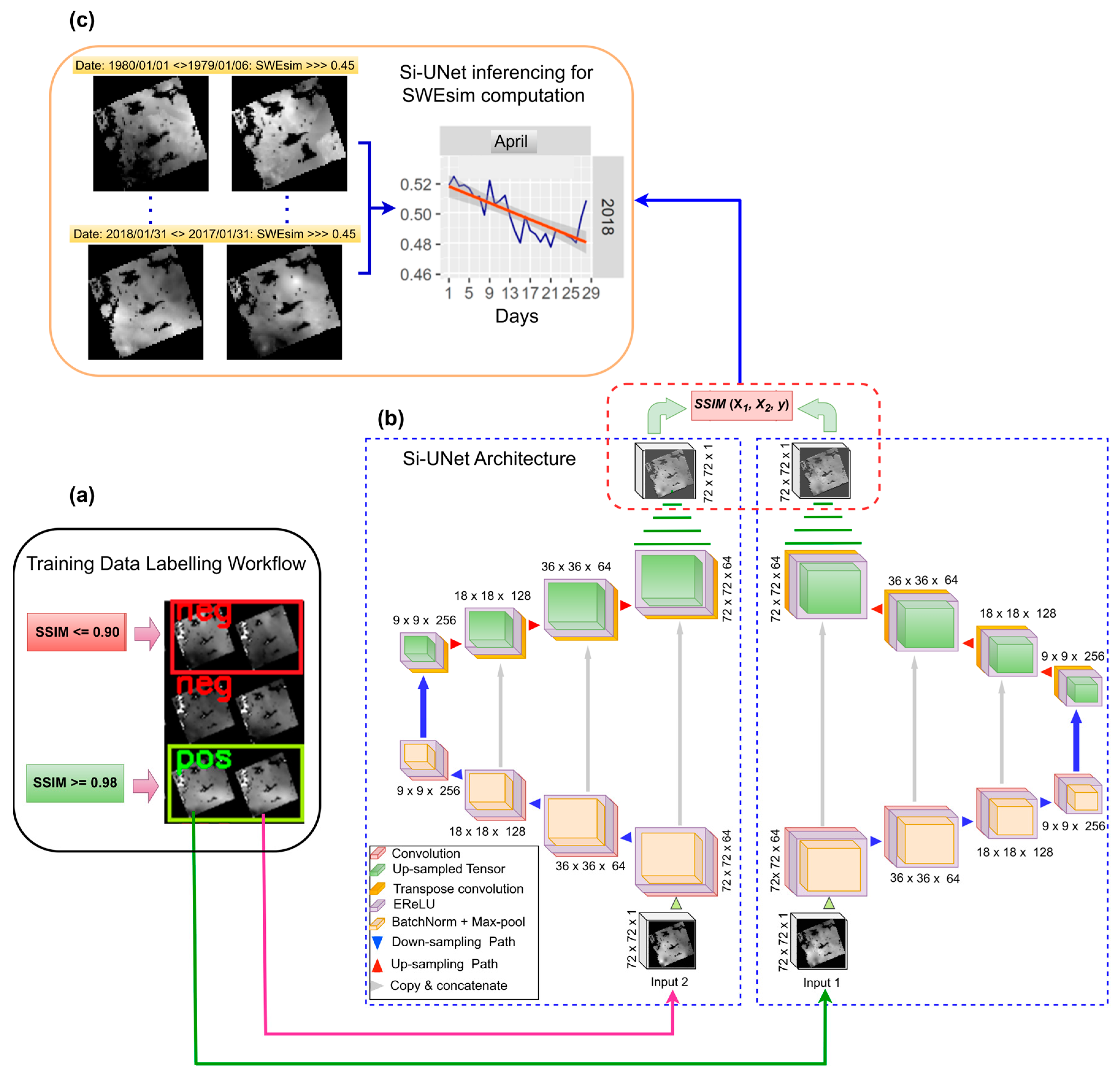
3.3. Siamese U-Net Model Architecture

The Siamese U-Net architecture and SWE similarity computation are presented in Figure 2b,c. The Siamese network allowed the model to learn shared feature representations from two input images. At the same time, the U-Net with an encoder–decoder architecture and skip connections simultaneously facilitated the learning of significant features for SWE representation and reconstruction. Thus, the Siamese U-Net network learned spatial structures that characterize SWE distribution and spatial processes generating SWE. We note that although the temporal resolution of the data was high (i.e., daily), the spatial resolution was coarse. Therefore, the choice of the filter (kernel) was crucial for accurate SWE detection. The receptive field (RF) of deep learning models tends to increase by several folds with layer depth, culminating in higher layers having relatively high RF. This necessitates a thoughtful choice of filter size. Beginning feature extraction with a large filter (e.g., 5 × 5) will result in the RF growing extensively in deeper layers. Lower layers of the model extract low-level features that encode more local information, whereas higher layers tend to extract abstract or global features. Therefore, smaller filters will slow the rapid growth of the RF, leading to the extraction of fine-grained features. We, therefore, adopted a 3 × 3 filter.

3.4. Training Data and SWE Labelling

Before labelling the SWE data, a thorough visual inspection was conducted to discern the spatial–temporal variability of daily SWE. We discovered that SWE data that differed by one day tended to vary locally; however, global differences were less pronounced. Therefore, two SWE maps were labelled as positive pairs (No Change) if their sampling interval was one day apart. Conversely, pairs of SWE maps were labelled as negative pairs if their sampling dates were two or more days apart. We note that the inherent spatial–temporal variability of snow parameters rendered it challenging to objectively dichotomize a pair of SWE maps. For example, the SWE maps in April sometimes appeared to be substantially different despite being sampled at one-day intervals. It is also important to emphasize that there were timestamps in which the SWE maps were two or more days apart but could not be distinguished, especially in February and March. To circumvent these challenges, the SSIM index was adapted to objectively label the data, with support from human inspection.
To empirically derive a threshold at which the SSIM index estimates of SWE similarity coincided with human judgment, we examined the similarity distribution of SWE data over a range of SSIM index values. At SSIM index values ≥ 0.98, the SWE map pairs were similar and could not be easily dichotomized by human observers. In contrast, SSIM values ≤ 0.9 were characteristics of SWE map pairs that were easily distinguishable (i.e., changed/different maps). Accordingly, these SSIM index values were adopted as threshold values for dichotomizing SWE pairs as positive (i.e., No Change) and negative (i.e., Change). The SWE map pairs with SSIM values ranging from 0.91 to 0.97 were excluded from the training sample to avoid confusion during model training. It is important to emphasize that although excluding SWE map pairs in which the SSIM index values were between 0.91 and 0.97 risked reducing the sample size and critical values, this approach decreased the number of ambiguous labels during model training and accuracy assessment.
The data labelling and concept framework for the proposed Si-UNet model with SWE over the cold regions of Canada is shown in Figure 2a,b. SWE data from 1979 to 2001 were employed for model development, whereas data from 2002 to 2018 formed an independent validation sample. Figure 2a depicts the input data, which consisted of 72 × 72 pixel SWE maps covering the cold regions of Canada.

3.5. SSIM Index Properties

The expression for the SSIM index, proposed by Wang et al. [38], is given below.
S S I M x , y = 2 µ x µ y + C 1 2 σ x y + C 2 µ x 2 + µ y 2 + C 1 σ x 2 + σ y 2 + C 2  
w h e r e   µ x   a n d   µ y   represent the mean of a block of pixels in images x and y, respectively; σ x 2 and σ y 2 are respectively the variances of x and y  σ x y is the x and y covariance term; C 1   a n d   C 2 are stabilizing constants to account for the saturation effects of the human visual system. For further details on the SSIM index, we refer readers to the mathematical formulation presented in [38].
The SSIM index exhibits symmetry :   S S I M x , y = S S I M y , x .   Therefore, the SSIM index value is insensitive to the order in which the similarity of the output of the 2D SWE generated by the Si-UNet is evaluated. Additionally, the upper bound of the SSIM index, S S I M x , y = 1 , is attained if and only if (i.i.f) a pair of SWE maps are identical copies. In contrast, the lower bound of the SSIM index, S S I M x , y = 0 , occurs when a pair of SWE maps is distinctively opposite (e.g., snow versus zero-snow area). Nonetheless, given the temporal dimension of the data and the magnitude of inherent spatial variability in the distribution of SWE, it is highly improbable that these two scenarios will ever be established for any bi-temporal SWE maps. Consequently, the SSIM index value is constrained to follow the expression 0 S S I M 1 . Thus, the upper bound of the SSIM index aligns with the margin parameter m = 1 in the contrastive loss function, rendering the optimization task via contrastive loss an effective technique.

3.6. Combining the SSIM Index and the Contrastive Loss Function

Contrastive loss has been proven to be effective for learning tasks that involve dichotomizing a pair of data points. The learning objective compels similar data point pairs to obtain a higher similarity score and assigns a lower score to a set of dissimilar data pairs [39]. This aligns with the notion of maximizing the SSIM index value for similar (No Change) and minimizing the SSIM index value for unlike pairs (Change), as illustrated using the notations below:
x i , x j = max | S S I M x i , x j | ,   i = j min | S S I M x i , x j | , i   j
where i ,   j are indexes for a set of 2D feature maps, and S S I M · denotes the SSIM index.
The contrastive loss function written to incorporate the SSIM index is given as follows:
L c = ( 1 Y ) 1 2 ( S S I M x , y ) 2 + Y 1 2   max m S S I M x , y ,   0 2  
where L c denotes contrastive loss, m and S S I M are the margin and the SSIM index, respectively; x , y denotes a pair of SWE images; and Y represents the image pair labels. Note that for positive pairs (No Change), Y = 1 (i.e., Y = 1 | { i = j } ), and for negative pairs, (Change), Y = 0 (i.e., Y = 0 | { i   j } ). We note that the SSIM’s upper bound is 1, which aligns with the margin parameter m = 1 , often adopted for the contrastive loss function. In the next section, we decompose the contrastive loss to illuminate how the SSIM index fits into the objective function’s optimization paradigm.
It is worth noting that at each epoch, the SSIM index values were incorporated into the contractive loss function for optimization. By substituting m = 1 into the second component of the contrastive loss function with the SSIM index, the expressions below are yielded:
m S S I M x , y = m 2 µ x µ y + C 1 2 σ x y + C 2 µ x 2 + µ y 2 + C 1 σ x 2 + σ y 2 + C 2
1 S S I M x , y = 1 2 µ x µ y + C 1 2 σ x y + C 2 µ x 2 + µ y 2 + C 1 σ x 2 + σ y 2 + C 2
The SSIM index expression, after mean reduction of x and y , is simplified as follows:
1 S S I M x , y = 1 2 σ x y + C 2 σ x 2 + σ y 2 + C 2
Thus, the covariance term σ x y , which encodes similarities or differences in the spatial structure between a pair of SWE maps being compared, is amplified.
Given the “No Change” scenario, where Y = 1 (i.e., Y = 1 | { i = j } ), the first half of the contrastive loss expression (Equation (3)), ( 1 Y ) 1 2 ( S S I M x , y ) 2 , is nullified as it becomes 0. The second component, Y 1 2   max m s i m ,   0 2 , is then optimized, as illustrated below.
L c = 1 1 2   max 1 S S I M x , y ,   0 2
Therefore, if the image pairs are true “No Change” pairs, the SSIM value is expected to be high (i.e., near 1). Consequently, according to this equation, the model’s loss will be significantly reduced (i.e., L c 0 ) for SSIM values close to 1.
For scenarios of “Change”, where Y = 0 (i.e., Y = 0 | { i   j } ), the first component in Equation (3), ( 1 Y ) 1 2 ( S S I M x , y ) 2 , is optimized, while Y 1 2   max m S S I M x , y ,   0 2 becomes zero and is nullified accordingly.
L c = ( 1 0 ) 1 2 ( S S I M x , y ) 2
If the image pairs are true “Change” pairs, the SSIM value is expected to be very low (i.e., close to 0). As a result, the model’s loss will again be low (i.e., L c 0 ) for SSIM values near 0. Intuitively, according to the contrastive loss function, it follows that the model’s losses will increase i.i.f the computed SSIM value is high (near 1) but the image pairs are labelled as “Change” (False Change). In contrast, the model’s losses will increase i.i.f the image pairs are labelled as positive (“No Change”) but the SSIM value turns out to be low (False No Change).

3.7. Model Architecture, Loss Function, and Similarity Metrics

To illustrate the utility of the SSIM index and contrastive loss combination, we compared this formulation with binary cross-entropy (BCE) loss and the Euclidean distance (ECD) metric. BCE was further examined in combination with the SSIM index and the ECD metric. We compared the loss function and similarity score combination under varying model architectures and parameters. The proposed Si-UNet, the U-Net with an attention module (Si-Att-UNet), and the base CNN model with a fully connected last layer were chosen for comparison. We computed the true positive rate (TPR), true negative rate (TNR), false positive rate (FPR), false negative rate (FNR), precision (PR), F1 score, and overall accuracy (OA) to assess the models’ prediction of SWE similarity and change. The models’ accuracy was evaluated at a 40–70% confidence threshold. The TPR represents the proportion of SWE map pairs that were correctly classified as No Change (i.e., similar), whereas the TNR represents the proportion that were accurately classified as Change (i.e., dissimilar). Accordingly, the FPR represents the SWE maps that were labelled as Change pairs but were misclassified as No Change instances, while the FNR approximates the SWE map pairs that were labelled as No Change pairs but were misclassified as Change instances. The equations for the accuracy metrics are presented in Appendix C. Furthermore, qualitative analysis and visualizations of change maps were employed to investigate the models’ similarity and change attribution behaviors.

3.8. Deriving Time Series SWE Similarity Vectors

Once trained and independently validated, the Si-UNet can be deployed to derive time series vectors for daily, monthly, and yearly SWE similarity, denoted as SWEsim. To compute the yearly SWEsim, SWE data in corresponding months were compared across successive years using the Si-UNet model. For example, to derive SWEsim trends for January from 1979 and 2018, Si-Unet received time series SWE data in January and output SWEsim by sequentially pairing the yearly SWE maps as follows: SWE1979 versus SWE1980, SWE1980 versus SWE1981, and SWE1981 versus SWE1982, until the end of the time series length (i.e., 2018). Reformulating the comparison equation in terms of mathematical notations yielded an SWEsim vector as follows:
S W E s i m Z i   Z n = S i U N e t S W E Z i j 1 , j 2 , j 3 j 31 , S W E Z i + 1   j 1 , j 2 , j 3 j 31
where j 1   to j 31   denote 1 January to 31 January SWE data, and Z represents the corresponding year. Such a comparison prompted the Si-UNet model to address a visual question of whether SWE data sampled in the most recent year, Z i   ,   and the preceding year, Z i 1 , were different. More specifically, the model answered the question of whether the SWE data observed on 1 January 2017 significantly differed from the SWE data observed on 1 January 2018. The Mann–Kendall (MK) test and linear regression were performed on the resultant S W E s i m vector to portray trends in [15,40]. For the MK test, the SWEsim vector for each year was used as input to estimate the parameter tau, whose sign determines the slope direction. Given that MK statistics do not quantify the magnitude of the underlying trend, linear regression was used to regress the SWEsim vector conditioned on years (i.e., changes in the SWEsim vector over the years).

4. Results

4.1. Ablation Studies

Table 1 summarizes the models’ performance under combinations of loss function, similarity, and accuracy metrics. We report the confidence thresholds under which each model’s performance was at its optimum. We note that the base CNN was not tested on the SSIM index since the fully connected layer output is a vector. The base CNN model and our Si-UNet, trained with BCE and ECD, recorded the lowest TPR and TNR. While the Si-UNet performed slightly better in the TPR, the base performance was high for the TNR. Overall, both models recorded identical F1 scores. With the BCE and SSIM index combination, it can be observed that our Si-UNet and the Si-Atte-UNet required a high threshold (i.e., 70%) to optimize their performance. Our Si-UNet excelled at TPR detection, whereas the Si-Att-UNet, with the highest number of parameters, performed marginally better in TNR detection. When substituting the BCE with the contrastive loss, the models’ confidence threshold for optimal detection decreased to 50%. Again, our Si-UNet performance improved in TPR detection, while that of the Si-Att-UNet was slightly higher for TNR detection.
Figure 3 presents a sample of FPR and FNR detections. Using the positional index for each input pair, we sampled a set of FPR and FNR detections to visualize the models’ similarity and change attribution behaviors with varying loss functions (i.e., BCE and contrastive loss) and similarity score metrics (i.e., ECD and the SSIM index). We used red rectangles to denote the regions that probably fooled the models into making wrong decisions. The green rectangles, on the other hand, highlight regions that are similar, but the models appeared to have disregarded the pixels in the decision process. The base CNN model and our Si-UNet, trained with BCE and ECD, tended to consistently record substantial proportions of FNR and FPR. These false detections can be easily recognized by human experts. In Figure 3a,c, the base CNN and our Si-UNet attributed higher similarity scores (0.6–0.64) to SWE maps that were labelled as Change pairs. Contrarily, in Figure 3b,d, the models attributed lower scores (0.17–0.19) to SWE maps that were labelled as No Change instances. By introducing the SSIM index, the FPR and FNR detections decreased substantially. Nevertheless, in Figure 3e,g, our Si-UNet and the Si-Att-UNet assigned high scores (0.71) to SWE maps that were Change pairs (i.e., negative samples). It can also be observed that the Si-UNet assigned a high score to the negative pair in Figure 3f. The FNR detections are depicted in Figure 3h,i for the Si-Att-UNet with BCE and contrastive loss combinations. The model attributed 0.5 and 0.6 to the SWE map pairs, as shown in Figure 3h,i, respectively. Although the SWE maps appear similar, with few pixel differences highlighted in the red rectangles, they were labelled as No Change pairs (i.e., positive samples).

4.2. A Comparison of Monthly Changes in SWE Distribution over 5 Years

Figure 4 and Figure 5 present combined violin and box plots illustrating the distribution of SWE similarity derived from comparisons of SWE between consecutive years, from January to April. Higher SWE values signify less significant change; conversely, lower values reflect pronounced changes in SWE between the years compared.

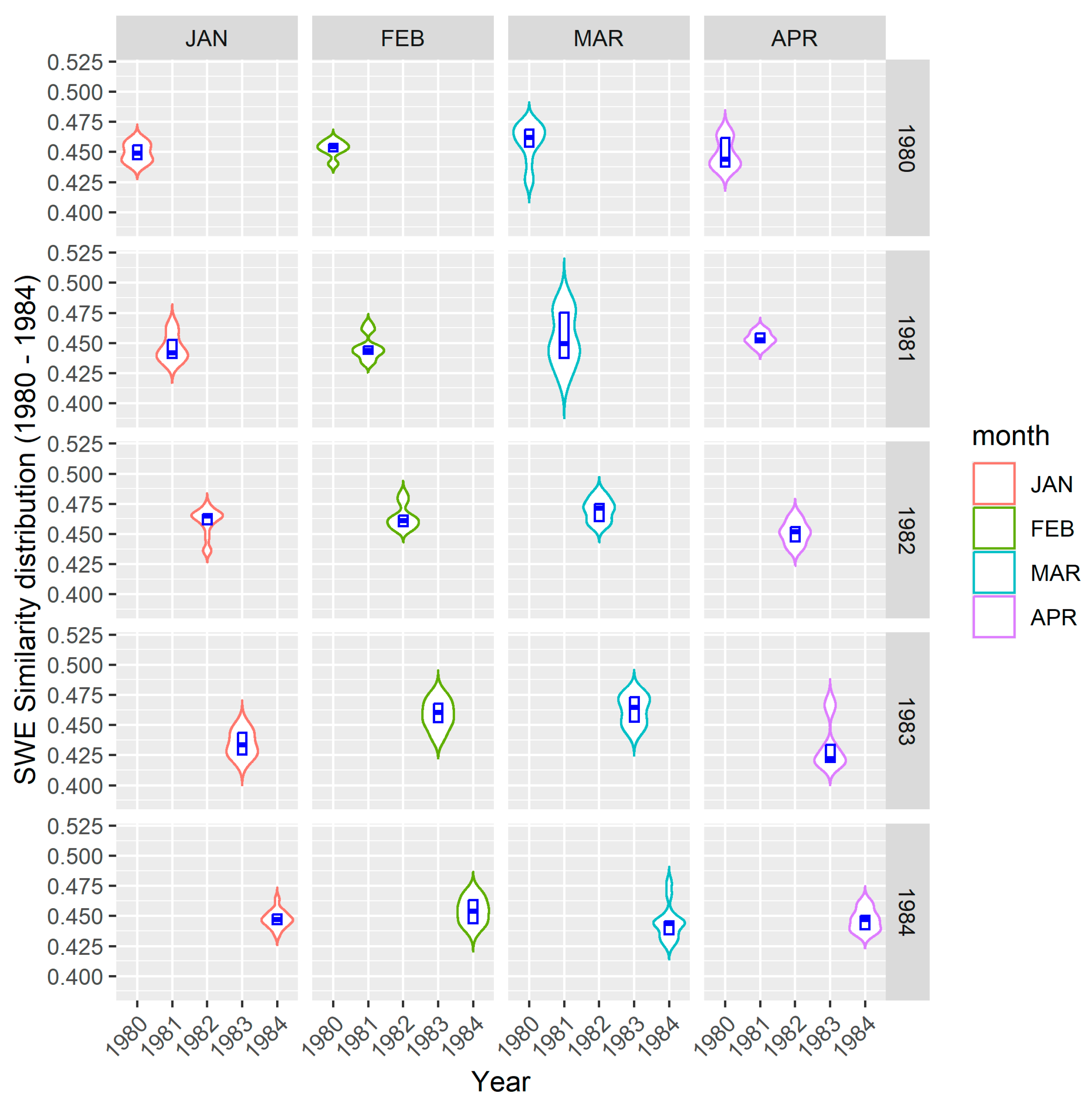
4.2.1. SWE Distribution—1980 to 1984

Figure 4 depicts a 5-year distribution of changes in SWE. The median SWEsim values for March appeared to be the highest. Aside from 1984, all the preceding years recorded a median similarity of over 0.45. April had the lowest median similarity. While all the months portrayed prominent dispersion over the years, the SWEsim in February appeared to be more uniform from 1980 to 1982.

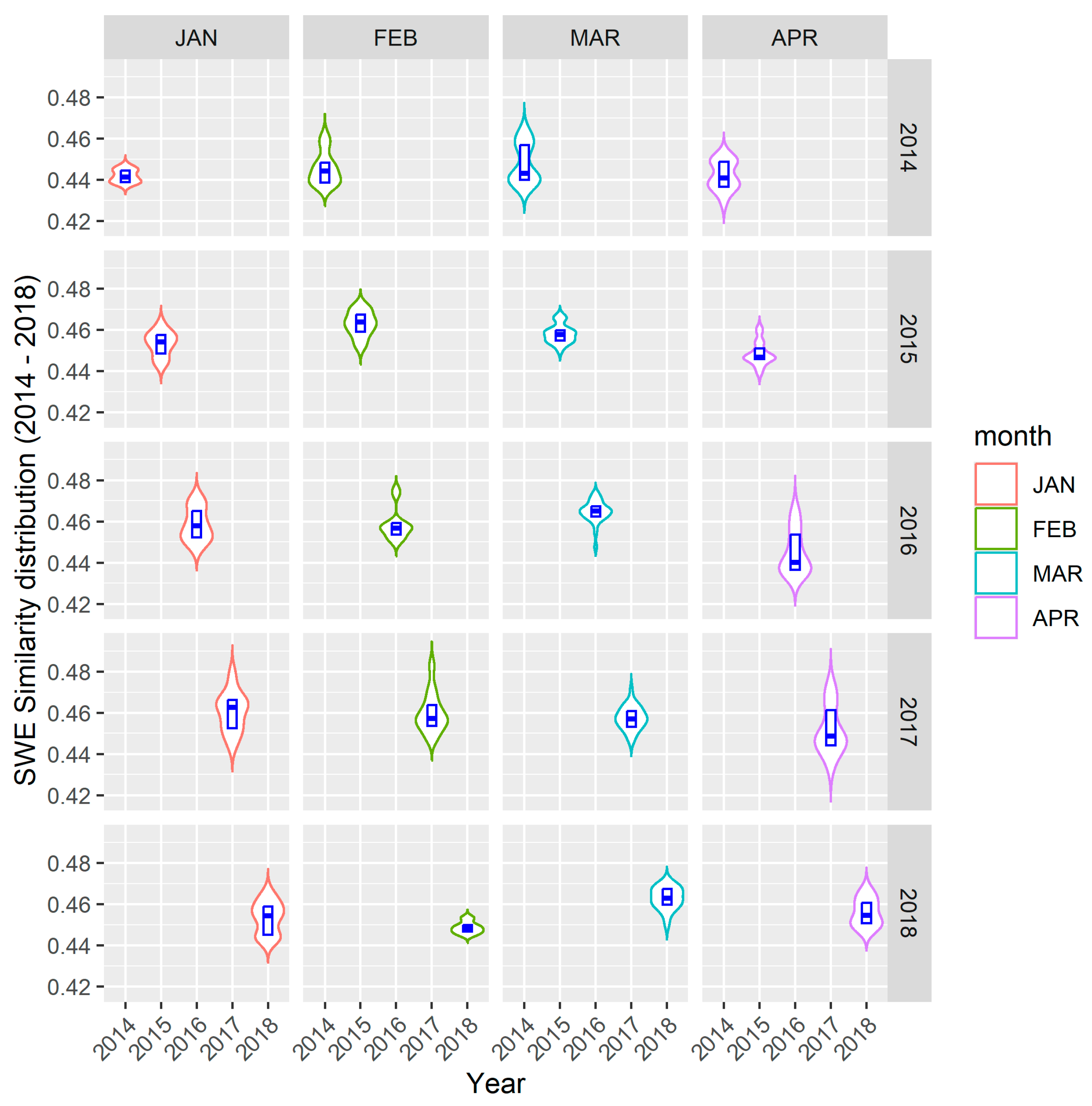
4.2.2. SWE Distribution—2014 to 2018

Figure 5 summarizes the SWE distribution between 2014 and 2018. As can be discerned from the figure, 2014 incurred the lowest SWEsim values for all the months (i.e., January–April). Given that the 2014 distribution was derived from a comparison with 2013 SWE data, it implies that the spatial structure characterizing the distribution of SWE in 2013 and 2014 was distinctively different. March exhibited the highest SWEsim values, followed by February and January. It is important to note, however, that January and April SWEsim largely depicted a bimodal distribution with high dispersion.

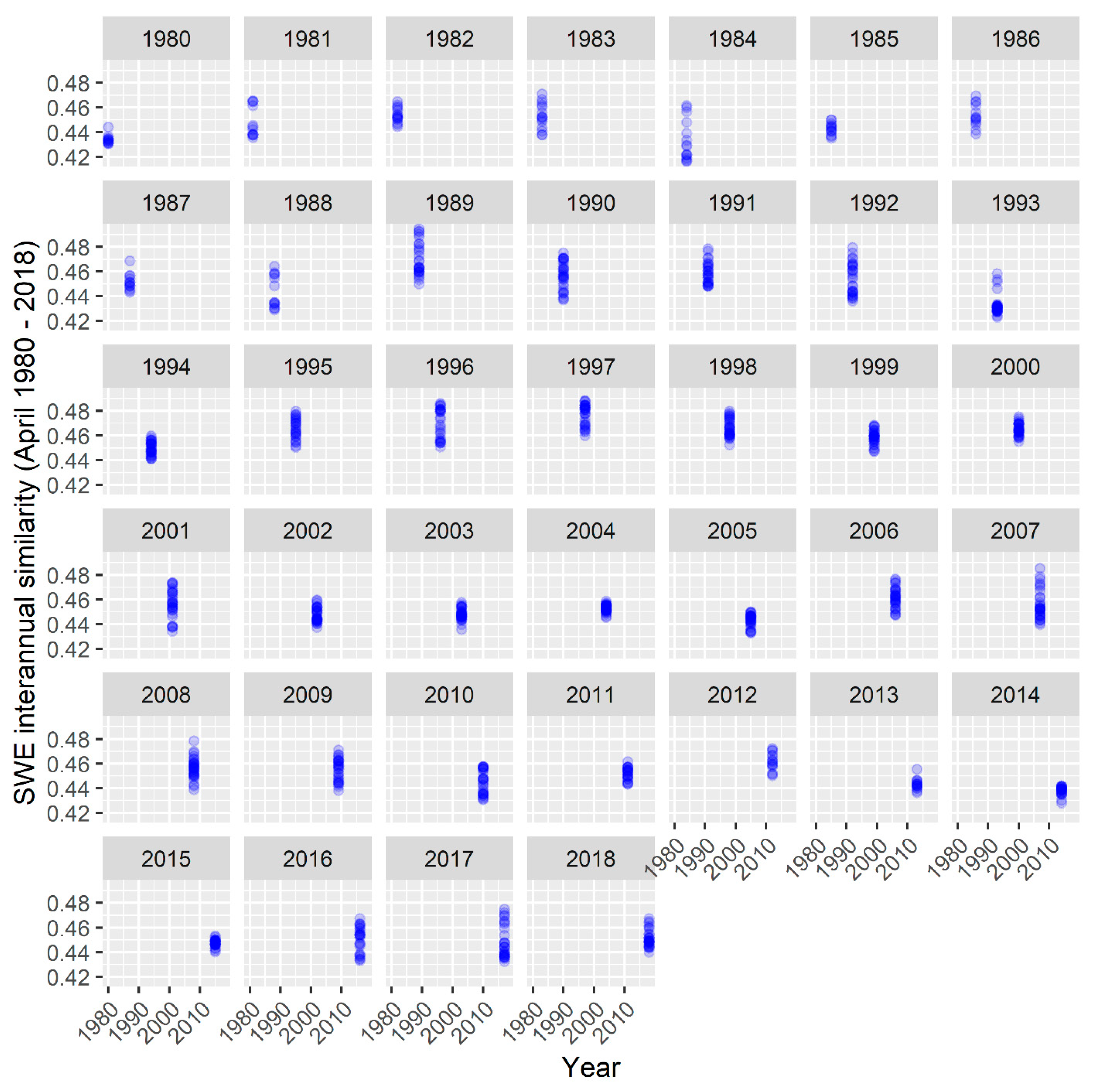
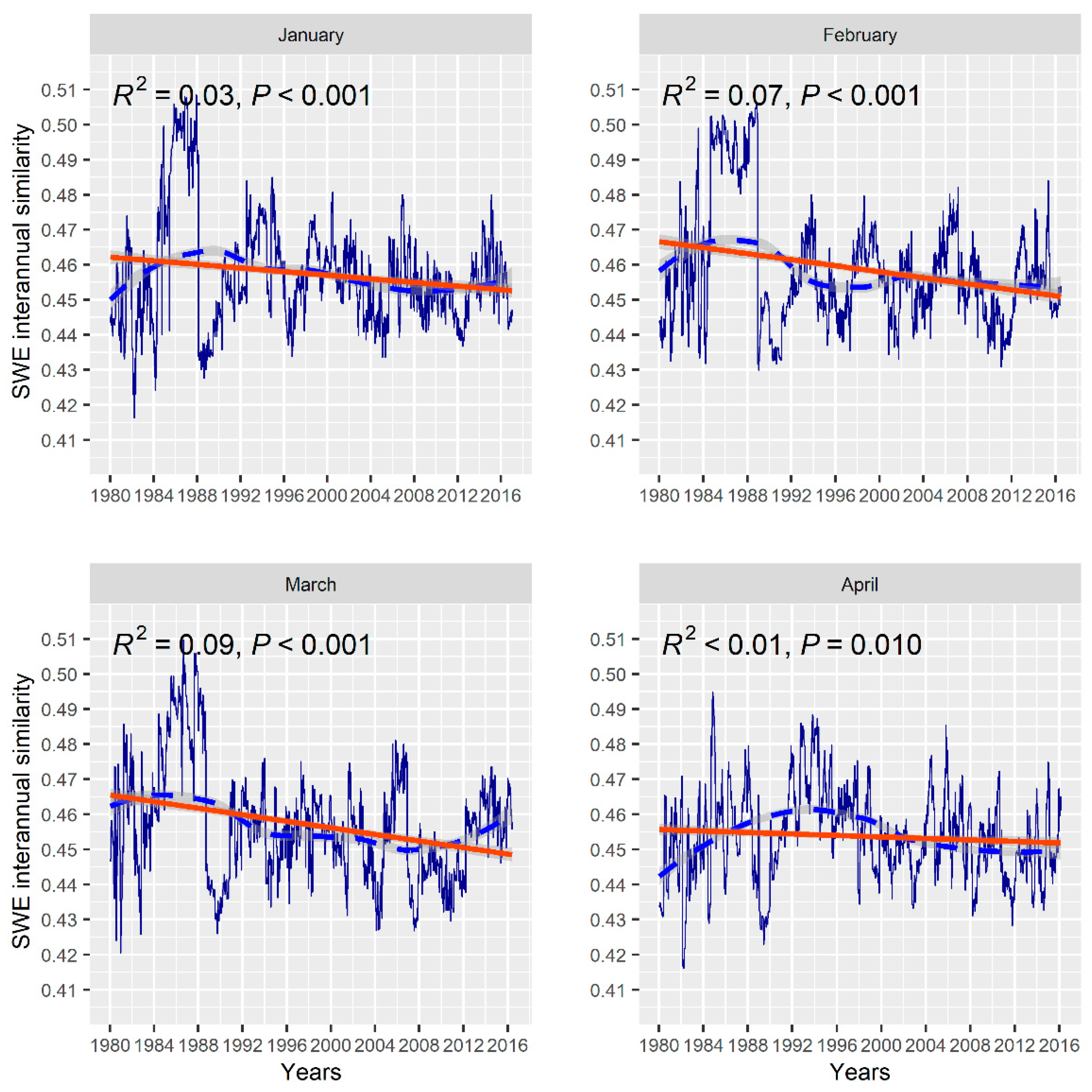
4.3. Interannual SWE Trends—1979 to 2018

Figure 6 depicts SWE trends from 1970 to 2018. The Mann–Kendall test results suggest a statistically significant negative or decreasing monotonic trend (tau < 0) in all the months. However, March incurred the highest rate of SWE decline (R2 ≈ 0.1, p-value < 0.05). Table A1 (see Appendix A) presents the statistics derived from the trend tests. The statistics, including the S, tau, and p-values, were obtained using the MK test, while the R2 values were derived from linear regression. On average, the SWEsim values were higher in the earlier years (i.e., 1979–1988). The later years (i.e., 1988–2018) were dominated by low SWEsim values.

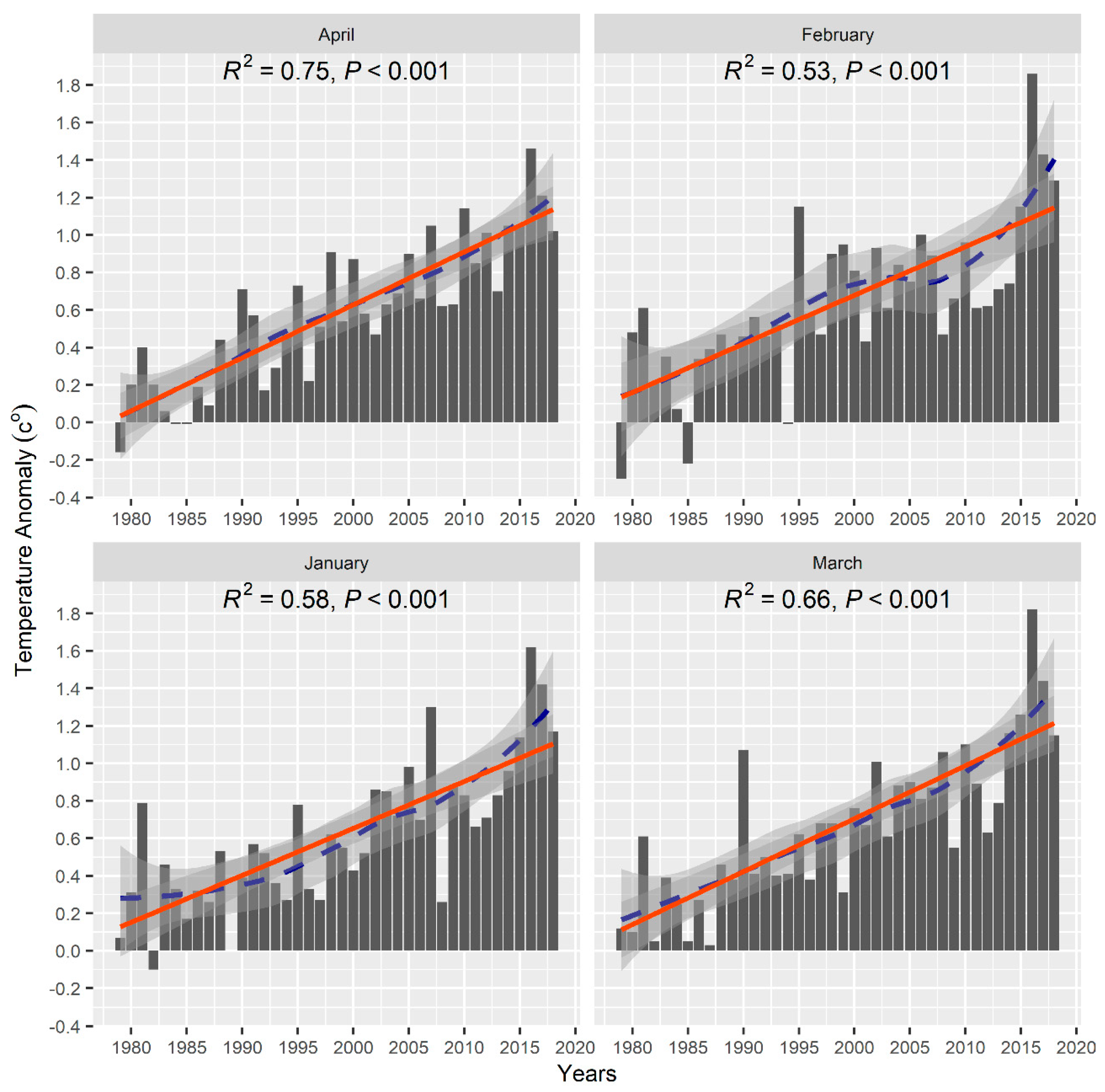
4.4. Northern Hemisphere Temperature Anomalies

In Figure 7, we present the National Oceanic and Atmospheric Administration (NOAA) mean monthly temperature anomalies from January to April. Comparing Figure 6 and Figure 7, it can be deduced that a decreasing pattern of SWE similarity coincided with an increasing temperature anomaly. Although the temperature anomalies portrayed a growing trend, the lowest average monthly anomaly occurred between 1979 and 1989, whereas the later years exhibited relatively high temperature anomalies. It can be seen that March and April had the strongest positive trends and R2 values of 0.66 and 0.75, respectively.

5. Discussion

We developed a Si-UNet to detect spatial–temporal changes using GlobSnow’s SWE data across Canada’s cold regions. We investigated the change detection problem using image content similarity analysis, where highly similar pairs of images (e.g., SWE maps) are anticipated to yield high scores, and dissimilar pairs of images yield low scores. Therefore, a high similarity score denotes little or no significant change in the SWE. Low scores, on the other hand, are indicative of significant changes in the SWE. We deployed the SSIM index to objectively label the training samples. This workflow, including the model’s architecture, is depicted in Figure 2a–c. The SSIM index scales out the effects of contrast and illumination variability while preserving structural differences. The structural component highly correlates with underlying spatial–temporal processes (e.g., precipitation and temperature) that largely dictate snow dynamics.
Siamese networks have been shown to extract discriminative features for pattern recognition tasks [41]. However, the challenge encountered in our SWEsim computation warranted modifications to the model’s architecture and loss function. Consequently, we adopted the U-Net backbone, the SSIM index, and the contrastive loss function to capture the spatial–temporal variability between a pair of SWE images [35,38,39]. The model was guided by a computer vision metric, the SSIM index, to weigh structural changes higher than changes in the intensity and contrast in SWE images [38]. A comparison of our Si-UNet with the base CNN model and the UNet with attention modules provided evidence that the contrastive loss and SSIM index combination was effective for change detection in SWE. Using BCE loss and the ECD metric, both the base CNN and our Si-UNet were worse at TPR and TNR detection, with F1 scores of 83%. This suggests that, without careful selection of the loss function and score metrics, the base CNN model, with the lowest number of parameters, can compete with the U-Net. By maintaining the EDC metric and introducing the SSIM index, the Si-UNet performance improved by a margin of 16%. The BCE and ECD combination required the highest confidence threshold to optimize the models’ performance. Therefore, this loss and metric mixture reduced the models’ sensitivity to SWE similarities and differences. Figure 3e,g reveals the loss of sensitivity to perceptual differences among the SWE maps, resulting in FPR detection for our Si-UNet and the Si-Att-UNet. Although the models’ accuracy reached 99% at a 70% threshold, there was a trade-off between the threshold value and the proportion of FPR and FNR. The contrastive loss and the SSIM index provided the best model. Therefore, our Si-UNet and the Si-Att-UNet were both competitive, achieving a 99% F1 score at a 50% threshold. This also implies the models were highly sensitive to SWE similarities and differences. This observation is evident in Table 1 and Figure 3. For example, our Si-UNet recorded zero FNRs in Figure 3 (row 4, column 3). In Figure 3h,i, it can be seen that the Si-Att-UNet recorded FNRs; however, a close examination of the pixels, highlighted using rectangles, reveals an interesting pattern in the model’s attribution of similarity scores. Although the SWE maps were labelled as negative pairs, they exhibited little perceptual difference. The Si-Att-UNet was highly sensitive to fine-grain variabilities among the SWE maps, whereas our Si-UNet ignored such structural details. Therefore, the Si-UNet may have detected such structural changes as noise or less significant patterns. This variation in model sensitivity implies that the Si-UNet is a candidate model for interannual SWE trend analysis, while the Si-Att-UNet holds potential for daily SWE change analysis, where model sensitivity to fine-detail similarities and/or changes would be required to characterize daily SWE trends.
We demonstrated the Si-UNet’s potential to detect interannual changes in snow parameters by comparing the yearly SWE from January to April. The larger the value of SWEsim, the higher the similarity between a pair of SWE maps. In other words, the larger the SWEsim is, the smaller the magnitude of change between a pair of SWE maps. The distribution of SWEsim for January and April tended to be frequently bimodal (Figure 4 and Figure 5) and relatively more dispersive compared to February and March. The dispersion of SWEsim in January is characteristic of the variability in snow arrival and accumulation, whereas that in April is indicative of variability in yearly snow melt-off patterns. Snow begins to melt and retreat during April but tends to exhibit a spatially variable distribution [22]. The lower median SWEsim values for all the months in April accentuate this melt-off pattern. The Si-UNet model detected higher SWEsim values between 1980 and 1984 (Figure 4). Conversely, lower SWEsim values were observed between 2014 and 2018 (Figure 5). Climate change and global warming phenomena are known to significantly affect precipitation and surface temperature, which in turn drive snowfall events [6,10], resulting in declining snow accumulation.
The distribution of monthly changes in the SWE within each year can provide informative insight into snow evolution in response to climate regime variability. To link the spatial–temporal variability of snow parameters to climate variables, we compared land and sea surface temperature (LSST) and precipitation anomalies reported by the NOAA in the NH for the corresponding years, from 1980 to 1984 and from 2014 to 2018 (Figure 7) [42]. Temperature anomalies were relatively low between 1980 and 1984. In contrast, high temperature anomalies were detected between 2014 and 2018. As expected, an inverse relationship was found between the SWEsim and LSST anomalies. The SWEsim remained high from 1980 to 1984 for all the months; this temporal window corresponds with the periods in which LSST anomalies were relatively low. The values of SWEsim, however, decreased steadily after 1988, when temperature anomalies continued to increase. These findings are consistent with extensive studies of the NH snow cover response to surface temperature [6,10,43,44].
Temperature and precipitation are key climate variables known to have a profound influence on snow dynamics [44,45,46,47]. This study found a reasonably consistent pattern in the relationship between SWE and NOAA’s climate anomalies. However, there was a stronger correlation between SWE decline and temperature anomalies than precipitation anomalies. Overall, precipitation in January exhibited the strongest relationship with SWE decline [42]. However, it is worth noting that spatial processes, such as temperature and precipitation, do not act at the same spatial scales; therefore, their effects on the spatial patterns of SWE variability will require analysis at the relevant scales to understand their impact on the snow regime [2,48]. Furthermore, non-climatic related variables can complicate trends in SWE variability [49,50].
The Mann–Kendall trend test and linear regression results confirm the negative SWE trends from 1980 to 2018. Although all the years depicted a negative or declining interannual SWE, the trend was statistically more significant in March. The Si-UNet detected the steepest SWE decline or change in March (R2  0.1, p-value < 0.05) (Appendix A, Table A1). All the other months portrayed a statistically significant reduction in the SWE, yet had weaker R2 values. This negative trends align well with previous studies that discovered a significant reduction in the SWE, SD, and SE over the NH, especially in peak snow months, such as March [5,8,22]. It is worth noting that our analysis utilized yearly SWE data to estimate the SWEsim. Therefore, the weak R2 and tau values reported may be attributed to small interannual variability in the SWE, as pointed out in [17], especially during peak snow months. For instance, analyses in which averages of SWE and decadal reference periods were used have reported stronger SWE trends [7,8,22].
We reiterate that despite the relatively weak R2 for the April SWE trend, it incurred the lowest SWEsim values (Appendix B, Figure A1). This signifies that April SWE may have been largely impacted by climate-forcing agents (e.g., temperature and precipitation) [4]. A significant decline in April SWE has been reported in the Western United States [21]. Furthermore, the high dispersion observed in the April SWE distribution emphasizes the oscillatory impact of climate-forcing agents on snow melt-off across space and time. It has been shown that snow and ice cover in Canada is decreasing over time, with inherent seasonal and regional variability, largely attributable to surface temperature [51]. Together, the negative slope of March SWEsim and the lower median SWEsim values for April portend earlier snowmelt and shorter winter season length in the NH [52,53]. This presents a worrying trend, given that snow cover duration in winter is crucial for sustaining water resources, particularly in the cold regions of Canada, where snowmelt represents a vital source of freshwater and outdoor leisure activities, such as skating [48,54].

6. Conclusions

Our study has demonstrated the utility of combining computer vision metrics and deep learning methods to detect spatial–temporal variability in SWE. The SSIM-guided Si-UNet model detected instances of “No Change” (i.e., high SWEsim values) and instances of “Change” (i.e., low SWEsim values) with a 99% F1 score at a 50% confidence threshold, an increase of 16% compared to the Si-UNet with BCE loss and ECD metric. However, at lower confidence thresholds (e.g., 40–45%), the model yielded a substantial proportion of false positives and false negatives, highlighting the challenging nature of the change detection problem in SWE. It is essential to reiterate that without the SSIM index and contrastive loss, higher confidence threshold values (e.g., 70%) are required to realize improved model performance. Additionally, the base CNN model and the Si-UNet with BCE loss and ECD metric performed poorly in detecting instances of similar and changed SWE. We note that the U-Net model with the attention module (i.e., Si-Att-UNet) possesses high sensitivity to fine-grain structural changes in SWE and is a candidate model for daily SWE change detection.
Our analysis of SWEsim and LSST revealed an inverse relationship, suggesting the impacts of temperature on SWE decline in the cold regions of Canada. This decline was more pronounced after 1988, when LSST anomalies continued to rise exponentially. March SWEsim exhibited a strong negative trend compared to January, February, and April. However, the values of SWEsim in April tended to be the lowest, indicating the severity of the impacts of temperature and precipitation anomalies on the snow regime in April. The distribution of SWEsim values in January and April was more dispersed. With progressive climate change and global warming events, the SWEsim may decrease remarkably in January and April. If this is not coupled with a shift in snow arrival and retreat time, then it could imply a reduction in the winter season length.
The major limitations of our study are twofold: (a) employing the GlobSnow SWE and NOAA datasets, and (b) using the SSIM index and the Si-UNet model. Although the GlobSnow v3.0 data are of high temporal resolution, their coarse spatial resolution (i.e., 25 km × 25 km) limits the analysis of changes in snow at local scales. The NOAA climate data represent monthly average temperature and precipitation over the NH. Therefore, the temporal resolution mismatches the SWE data, and the changes in the climate variables may not accurately correlate with changes in SWE. High spatial and temporal resolution datasets will offer more insight into changes in the snow regime. The SWE data also exclude snow cover in mountainous regions; therefore, snow processes at high altitudes cannot be studied. Furthermore, as pointed out earlier, between 1979 and 1987, the SWE data were sampled every other day, resulting in approximately 14 data points for each month. This temporal discontinuity likely introduced bias in the SWEsim values estimated between 1979 and 1987. Lastly, bias correction is required to ensure that the SWE data accurately reflect true changes in the nominal SWE values; however, it remains challenging to perfectly account for uncertainties and systematic errors in the SWE data products [55,56].
The limitations of the SSIM index and our Si-UNet stem from the fact that they do not offer quantitative estimates of SWE similarity in terms of the nominal values of SWE (i.e., how similar a pair of SWE maps is in millimetres). For example, the SWEsim values estimate similarity from zero (low) to one (high); however, this is not equivalent to SWE similarity in millimetres. Directly quantifying the SWE similarity or change could also provide more valuable insight into the decline of snow during the winter. Additionally, extending this analysis to other regions in the NH could provide an informed understanding of the impact of climate variables (e.g., temperature and precipitation) on the snow regime and cryosphere processes at broader spatial scales beyond the cold regions of Canada. This will be the focus of our next analysis we intend to conduct in the future.

Author Contributions

Conceptualization, K.M.; methodology, K.M.; formal analysis, K.M.; writing, K.M.; original draft preparation, K.M.; review and editing, C.R.; funding acquisition, K.M. and C.R. All authors have read and agreed to the published version of the manuscript.

Funding

This research received funding from the Natural Sciences and Engineering Research Council of Canada.

Data Availability Statement

The data used to train the model are available at https://www.globsnow.info/swe/archive_v3.0/ (accessed on 1 December 2024). The authors also plan to make the sample data and the trained model available after the manuscript is accepted or upon request.

Acknowledgments

The authors would like to acknowledge the University of Windsor’s support in conducting this research.

Conflicts of Interest

The authors declare no conflicts of interest.

Appendix A

Table A1. Mann–Kendall test results and linear regression statistics.
MonthNStaup-Value R2
January1019–3.31 × 10⁴–6.37 × 10−22.31 × 10−33.0 × 10⁻²
February950–4.38 × 10⁴–9.72 × 10−27.34 × 10−67.0 × 10⁻²
March1019–8.16 × 10⁴–1.57 × 10−25.62 × 10−149.0 × 10⁻²
April940–3.47 × 10⁴–7.85 × 10−23.13 × 10−41.0 × 10⁻²

Appendix B

Figure A1. April SWE distribution from 1980 to 2018, showing SWEsim vectors’ values as blue dots for the corresponding years.
Remotesensing 17 01631 g0a1

Appendix C

R e c a l l T P R = T P T P + F N
P r e c i s i o n = T P T P + F P
F 1   s c o r e = 2 T P 2 T P + F P + F N
T N R = T N T N + F P
O A = T P + T N T P + T N + F P + F N

References

  1. Thackeray, C.W.; Derksen, C.; Fletcher, C.G.; Hall, A. Snow and Climate: Feedbacks, Drivers, and Indices of Change; Springer: Berlin/Heidelberg, Germany, 2019. [Google Scholar] [CrossRef]
  2. Schilling, S.; Dietz, A.; Kuenzer, C. Snow Water Equivalent Monitoring—A Review of Large-Scale Remote Sensing Applications. Remote Sens. 2024, 16, 1085. [Google Scholar] [CrossRef]
  3. Callaghan, T.V.; Johansson, M.; Brown, R.D.; Groisman, P.Y.; Labba, N.; Radionov, V.; Bradley, R.S.; Blangy, S.; Bulygina, O.N.; Christensen, T.R.; et al. Multiple effects of changes in arctic snow cover. Ambio 2011, 40 (Suppl. S1), 32–45. [Google Scholar] [CrossRef]
  4. Rupp, D.E.; Mote, P.W.; Bindoff, N.L.; Stott, P.A.; Robinson, D.A. Detection and attribution of observed changes in northern hemisphere spring snow cover. J. Clim. 2013, 26, 6904–6914. [Google Scholar] [CrossRef]
  5. Pulliainen, J.; Luojus, K.; Derksen, C.; Mudryk, L.; Lemmetyinen, J.; Salminen, M.; Ikonen, J.; Takala, M.; Cohen, J.; Smolander, T.; et al. Patterns and trends of Northern Hemisphere snow mass from 1980 to 2018. Nature 2020, 581, 294–298. [Google Scholar] [CrossRef]
  6. Mudryk, L.R.; Kushner, P.J.; Derksen, C.; Thackeray, C. Snow cover response to temperature in observational and climate model ensembles. Geophys. Res. Lett. 2017, 44, 919–926. [Google Scholar] [CrossRef]
  7. Brown, R.D.; Fang, B.; Mudryk, L. Update of Canadian Historical Snow Survey Data and Analysis of Snow Water Equivalent Trends, 1967–2016. Atmos. Ocean 2019, 57, 149–156. [Google Scholar] [CrossRef]
  8. Räisänen, J. Changes in March mean snow water equivalent since the mid-20th century and the contributing factors in reanalyses and CMIP6 climate models. Cryosphere 2023, 17, 1913–1934. [Google Scholar] [CrossRef]
  9. Cordero, R.R.; Asencio, V.; Feron, S.; Damiani, A.; Llanillo, P.J.; Sepulveda, E.; Jorquera, J.; Carrasco, J.; Casassa, G. Dry-Season Snow Cover Losses in the Andes (18°–40°S) driven by Changes in Large-Scale Climate Modes. Sci. Rep. 2019, 9, 16945. [Google Scholar] [CrossRef]
  10. Brown, R.D.; Robinson, D.A. Northern Hemisphere spring snow cover variability and change over 1922–2010 including an assessment of uncertainty. Cryosphere 2011, 5, 219–229. [Google Scholar] [CrossRef]
  11. Luojus, K.; Pulliainen, J.; Takala, M.; Derksen, C.; Rott, H.; Nagler, T.; Solberg, R.; Wiesmann, A.; Metsamaki, S.; Malnes, E.; et al. Investigating the feasibility of the globsnow snow water equivalent data for climate research purposes. In Proceedings of the 2010 IEEE International Geoscience and Remote Sensing Symposium, Honolulu, HI, USA, 25–30 July 2010; Volume 19, pp. 4851–4853. [Google Scholar] [CrossRef]
  12. Fontrodona-Bach, A.; Schaefli, B.; Woods, R.; Teuling, A.J.; Larsen, J.R. NH-SWE: Northern Hemisphere Snow Water Equivalent dataset based on in situ snow depth time series. Earth Syst. Sci. Data 2023, 15, 2577–2599. [Google Scholar] [CrossRef]
  13. Luomaranta, A.; Aalto, J.; Jylhä, K. Snow cover trends in Finland over 1961–2014 based on gridded snow depth observations. Int. J. Climatol. 2019, 39, 3147–3159. [Google Scholar] [CrossRef]
  14. Brown, R.D.; Brasnett, B.; Robinson, D. Gridded North American monthly snow depth and snow water equivalent for GCM evaluation. Atmos. Ocean 2003, 41, 1–14. [Google Scholar] [CrossRef]
  15. Gan, T.Y.; Barry, R.G.; Gizaw, M.; Gobena, A.; Balaji, R. Changes in North American snowpacks for 1979–2007 detected from the snow water equivalent data of SMMR and SSM/I passive microwave and related climatic factors. J. Geophys. Res. Atmos. 2013, 118, 7682–7697. [Google Scholar] [CrossRef]
  16. Räisänen, J. Snow conditions in northern Europe: The dynamics of interannual variability versus projected long-term change. Cryosphere 2021, 15, 1677–1696. [Google Scholar] [CrossRef]
  17. Kim, R.S.; Kumar, S.; Vuyovich, C.; Houser, P.; Lundquist, J.; Mudryk, L.; Durand, M.; Barros, A.; Kim, E.J.; Forman, B.A.; et al. Snow Ensemble Uncertainty Project (SEUP): Quantification of snow water equivalent uncertainty across North America via ensemble land surface modeling. Cryosphere 2021, 15, 771–791. [Google Scholar] [CrossRef]
  18. Urraca, R.; Gobron, N. Temporal stability of long-term satellite and reanalysis products to monitor snow cover trends. Cryosphere 2023, 17, 1023–1052. [Google Scholar] [CrossRef]
  19. Cheng, K.; Wei, Z.; Li, X.; Ma, L. Multi-Source Dataset Assessment and Variation Characteristics of Snow Depth in Eurasia from 1980 to 2018. Atmosphere 2024, 15, 530. [Google Scholar] [CrossRef]
  20. Hale, K.E.; Jennings, K.S.; Musselman, K.N.; Livneh, B.; Molotch, N.P. Recent decreases in snow water storage in western North America. Commun. Earth Environ. 2023, 4, 170. [Google Scholar] [CrossRef]
  21. Mote, P.W.; Li, S.; Lettenmaier, D.P.; Xiao, M.; Engel, R. Dramatic declines in snowpack in the western US. NPJ Clim. Atmos. Sci. 2018, 1, 2. [Google Scholar] [CrossRef]
  22. Zhang, Y.; Ma, N. Spatiotemporal variability of snow cover and snow water equivalent in the last three decades over Eurasia. J. Hydrol. 2018, 559, 238–251. [Google Scholar] [CrossRef]
  23. Dierauer, J.R.; Allen, D.M.; Whitfield, P.H. Climate change impacts on snow and streamflow drought regimes in four ecoregions of British Columbia. Can. Water Resour. J. 2021, 46, 168–193. [Google Scholar] [CrossRef]
  24. Santi, E.; Pettinato, S.; Paloscia, S.; Pampaloni, P.; Fontanelli, G.; Crepaz, A.; Valt, M. Monitoring of Alpine snow using satellite radiometers and artificial neural networks. Remote Sens. Environ. 2014, 144, 179–186. [Google Scholar] [CrossRef]
  25. Malik, K.; Robertson, C. Exploring the Use of Computer Vision Metrics for Spatial Pattern Comparison. Geogr. Anal. 2019, 52, 617–641. [Google Scholar] [CrossRef]
  26. Bromley, R.S.J.; Guyon, I.; LeCun, Y.; Sickinger, E. Signature Verification using a ‘Siamese’ Time Delay Neural Network. Adv. Neural Inf. Process. Syst. 1993, 6, 737–744. [Google Scholar] [CrossRef]
  27. Ronneberger, O.; Fischer, P.; Brox, T. U-Net: Convolutional Networks for Biomedical Image Segmentation. In Proceedings of the International Conference on Medical Image Computing and Computer-Assisted Intervention, Munich, Germany, 5–9 October 2015; Springer: Cham, Switzerland, 2015; pp. 234–241. [Google Scholar] [CrossRef]
  28. Zhang, J.; Lu, C.; Li, X.; Kim, H.J.; Wang, J. A full convolutional network based on DenseNet for remote sensing scene classification. Math. Biosci. Eng. 2019, 16, 3345–3367. [Google Scholar] [CrossRef]
  29. Cao, K.; Zhang, X. An improved Res-UNet model for tree species classification using airborne high-resolution images. Remote Sens. 2020, 12, 1128. [Google Scholar] [CrossRef]
  30. Thomas, E.; Pawan, S.J.; Kumar, S.; Horo, A.; Niyas, S.; Vinayagamani, S.; Kesavadas, C.; Rajan, J. Multi-Res-Attention UNet: A CNN Model for the Segmentation of Focal Cortical Dysplasia Lesions from Magnetic Resonance Images. IEEE J. Biomed. Health Inform. 2020, 25, 1724–1734. [Google Scholar] [CrossRef]
  31. Zhang, M.; Liu, Z.; Feng, J.; Liu, L.; Jiao, L. Remote Sensing Image Change Detection Based on Deep Multi-Scale Multi-Attention Siamese Transformer Network. Remote Sens. 2023, 15, 842. [Google Scholar] [CrossRef]
  32. Wu, L.; Wang, Y.; Gao, J.; Li, X. Where-and-When to Look: Deep Siamese Attention Networks for Video-Based Person Re-Identification. IEEE Trans. Multimed. 2019, 21, 1412–1424. [Google Scholar] [CrossRef]
  33. Yuan, P.; Zhao, Q.; Zhao, X.; Wang, X.; Long, X.; Zheng, Y. A transformer-based Siamese network and an open optical dataset for semantic change detection of remote sensing images. Int. J. Digit. Earth 2022, 15, 1506–1525. [Google Scholar] [CrossRef]
  34. Michal, D.; Eugene, V.; Gabriel, C.; Samuel, K.; Chris, P. The Importance of Skip Connections in Biomedical Image Segmentation. In Deep Learning and Data Labeling for Medical Applications; Springer International Publishing: Cham, Switzerland, 2016; pp. 179–187. [Google Scholar] [CrossRef]
  35. Tang, Y.; Cao, Z.; Guo, N.; Jiang, M. A Siamese Swin-Unet for image change detection. Sci. Rep. 2024, 14, 4577. [Google Scholar] [CrossRef] [PubMed]
  36. Canadian Environmental Sustainability Indicators. Environment and Climate Change Canada (2024). Canadian Environmental Sustainability Indicators: Snow Cover. Consulted on Month Day, Year. July 2024. Available online: www.canada.ca/en/environment-climate-change/services/environmental-indicators/snow-cover.html (accessed on 2 February 2025).
  37. Luojus, K.; Pulliainen, J.; Takala, M.; Lemmetyinen, J.; Mortimer, C.; Derksen, C.; Mudryk, L.; Moisander, M.; Hiltunen, M.; Smolander, T.; et al. GlobSnow v3.0 Northern Hemisphere snow water equivalent dataset. Sci. Data 2021, 8, 163. [Google Scholar] [CrossRef]
  38. Wang, Z.; Bovik, A.C.; Sheikh, H.R.; Member, S.; Simoncelli, E.P.; Member, S. Image Quality Assessment: From Error Visibility to Structural Similarity. IEEE Trans. Image Process. 2004, 13, 600–612. [Google Scholar] [CrossRef]
  39. Chopra, S.; Hadsell, R.; Lecun, Y. Learning a Similarity Metric Discriminatively, with Application to Face Verification. In Proceedings of the 2005 IEEE Computer Society Conference on Computer Vision and Pattern Recognition (CVPR’05), San Diego, CA, USA, 20–25 June 2005; pp. 539–546. [Google Scholar]
  40. Malik, K.; McLeman, R.; Robertson, C.; Lawrence, H. Reconstruction of past backyard skating seasons in the Original Six NHL cities from citizen science data. Can. Geogr. 2020, 64, 564–575. [Google Scholar] [CrossRef]
  41. Dey, S.; Dutta, A.; Toledo, J.I.; Ghosh, S.K.; Llados, J.; Pal, U. SigNet: Convolutional Siamese Network for Writer Independent Offline Signature Verification. July 2017. Available online: http://arxiv.org/abs/1707.02131 (accessed on 1 February 2025).
  42. NOAA National Centers for Environmental Information, Climate at a Glance: Global Time Series. Available online: https://www.ncei.noaa.gov/access/monitoring/climate-at-a-glance/global/time-series (accessed on 8 March 2025).
  43. Räisänen, J. Warmer climate: Less or more snow? Clim. Dyn. 2008, 30, 307–319. [Google Scholar] [CrossRef]
  44. Mudryk, L.; Santolaria-Otín, M.; Krinner, G.; Ménégoz, M.; Derksen, C.; Brutel-Vuilmet, C.; Brady, M.; Essery, R. Historical Northern Hemisphere snow cover trends and projected changes in the CMIP6 multi-model ensemble. Cryosphere 2020, 14, 2495–2514. [Google Scholar] [CrossRef]
  45. Erlat, E.; Aydin-Kandemir, F. Changes in snow cover extent in the Central Taurus Mountains from 1981 to 2021 in relation to temperature, precipitation, and atmospheric teleconnections. J. Mt. Sci. 2024, 21, 49–67. [Google Scholar] [CrossRef]
  46. Ishida, K.; Ohara, N.; Ercan, A.; Jang, S.; Trinh, T.; Kavvas, M.L.; Carr, K.; Anderson, M.L. Impacts of climate change on snow accumulation and melting processes over mountainous regions in Northern California during the 21st century. Sci. Total Environ. 2019, 685, 104–115. [Google Scholar] [CrossRef] [PubMed]
  47. Mankin, J.S.; Diffenbaugh, N.S. Influence of temperature and precipitation variability on near-term snow trends. Clim. Dyn. 2015, 45, 1099–1116. [Google Scholar] [CrossRef]
  48. Malik, K.; Robertson, C.; Roberts, S.A.; Remmel, T.K.; Jed, A. Computer vision models for comparing spatial patterns: Understanding spatial scale. Int. J. Geogr. Inf. Sci. 2022, 37, 1–35. [Google Scholar] [CrossRef]
  49. Kunkel, K.E.; Palecki, M.A.; Hubbard, K.G.; Robinson, D.A.; Redmond, K.T.; Easterling, D.R. Trend identification in twentieth-century U.S. snowfall: The challenges. J. Atmos. Ocean Technol. 2007, 24, 64–73. [Google Scholar] [CrossRef]
  50. Derksen, C.; Mudryk, L. Assessment of Arctic seasonal snow cover rates of change. Cryosphere 2023, 17, 1431–1443. [Google Scholar] [CrossRef]
  51. Mudryk, L.R.; Derksen, C.; Howell, S.; Laliberté, F.; Thackeray, C.; Sospedra-Alfonso, R.; Vionnet, V.; Kushner, P.J.; Brown, R. Canadian snow and sea ice: Historical trends and projections. Cryosphere 2018, 12, 1157–1176. [Google Scholar] [CrossRef]
  52. Klein, G.; Vitasse, Y.; Rixen, C.; Marty, C.; Rebetez, M. Shorter snow cover duration since 1970 in the swiss alps due to earlier snowmelt more than to later snow onset. Clim Chang. 2016, 139, 637–649. [Google Scholar] [CrossRef]
  53. Essery, R.; Kim, H.; Wang, L.; Bartlett, P.; Boone, A.; Brutel-Vuilmet, C.; Burke, E.; Cuntz, M.; Decharme, B.; Dutra, E.; et al. Snow cover duration trends observed at sites and predicted by multiple models. Cryosphere 2020, 14, 4687–4698. [Google Scholar] [CrossRef]
  54. Musselman, K.N.; Addor, N.; Vano, J.A.; Molotch, N.P. Winter melt trends portend widespread declines in snow water resources. Nat. Clim. Chang. 2021, 11, 418–421. [Google Scholar] [CrossRef]
  55. Kouki, K.; Luojus, K.; Riihelä, A. Evaluation of snow cover properties in ERA5 and ERA5-Land with several satellite-based datasets in the Northern Hemisphere in spring 1982–2018. Cryosphere 2023, 17, 5007–5026. [Google Scholar] [CrossRef]
  56. Mortimer, C.; Mudryk, L.; Derksen, C.; Luojus, K.; Brown, R.; Kelly, R.; Tedesco, M. Evaluation of long-term Northern Hemisphere snow water equivalent products. Cryosphere 2020, 14, 1579–1594. [Google Scholar] [CrossRef]
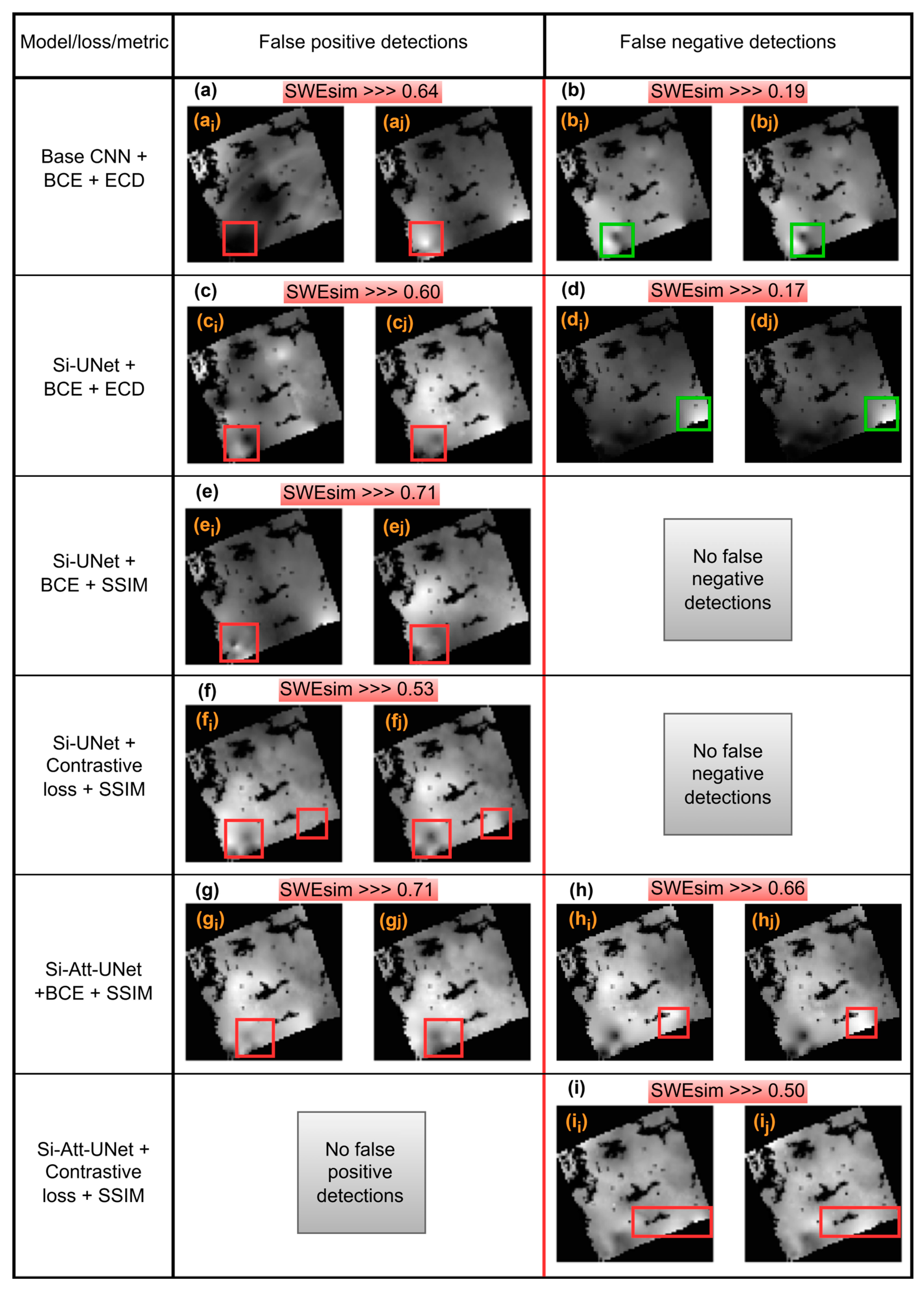
Figure 1. SWE distribution across the cold regions of Canada. A, B, and C represent Lake Athabasca, the Great Slave Lake, and the Great Bear Lake, respectively. Negative values (i.e., −1 and −2) denote water and mountain areas, as the GlobSnow data do not cover these features.
Remotesensing 17 01631 g001
Figure 2. (b) Si-U-Net architecture, (a) data labelling workflow, and (c) SWE similarly inferencing. The labelled 2D pair of SWE maps were assimilated by the pre-trained model for deconstruction and reconstruction in the encoder and decoder branches, respectively. The reconstructed SWE maps were compared to derive a SWE similarity vector (SWEsim) using the SSIM index as a scoring metric. A hypothetical graph of SWEsim is depicted in (c), where the blue line denotes SWE similarity and the orange line linear regressing trend line.
Remotesensing 17 01631 g002
Figure 3. FPR and FNR visualization with varying loss function and similarity metrics. False positive SWE pairs are (a)—(ai,aj), (c)—(ci,cj), (e)—(ei,ej), (f)—(fi,fj), and (g)—(gi,gj). False negative SWE pairs are (b)—(bi,bj), (d)—(di,dj), (h)—(hi,hj), and (i)—(ii,ij). Red rectangles denote regions that are different among SWE maps and green rectangles highlight similar regions.
Remotesensing 17 01631 g003
Figure 4. SWE distribution for years 1980–1984. Box plots are denoted in blue at the center of the violin plots. The SWE distribution captures the years when precipitation and temperature anomalies were low.
Remotesensing 17 01631 g004
Figure 5. SWE distribution for years 2014–2018. Box plots are denoted in blue at the center of the violin plots. It can be observed that the SWEsim for January and April continued to be more dispersed; however, the April SWEsim median values were comparatively low.
Remotesensing 17 01631 g005
Figure 6. A 40-year SWE trend in Canada’s cold regions from January to April. The dark blue lines represent time-series plots for SWEsim trends. Blue dotted lines represent LOESS fitting, and orange-red lines were derived from linear regression. The gray area around the trend lines denotes a 95% confidence interval.
Remotesensing 17 01631 g006
Figure 7. Land and sea surface temperature anomalies in the Northern Hemisphere. The blue-dotted and the orange-red lines denote LOESS fitting and linear regression trend estimates, respectively. The gray area around the LOESS and regression lines represents a 95% confidence interval. Positive temperature anomalies tended to dominate all months. The earlier years (e.g., 1979 to 1989) portrayed negative and low positive anomalies compared to the later years (e.g., 1990 to 2018).
Remotesensing 17 01631 g007
Table 1. Models’ performance with varying loss functions and similarity metrics.
Model
Architecture
Model
Parameters
Confidence
Threshold
Loss FunctionsSimilarity MetricsAccuracy Metrics
BCECont. LossECDSSIMTPRTNRPRF1-ScoreOA
CNN base1,773,19050%YesNoYesNo78.6595.5688.658390.38
Si-UNet 2,560,64650%YesNoYesNo87.589.7479.58389.05
Si-UNet 2,560,64670%YesNoNoYes10099.2398.299999.56
Si-Att-UNet8,134,59370%YesNoNoYes95.4999.8599.649898.51
Si-UNet 2,560,64650%NoYesNoYes10098.9397.639999.25
Si-Att-UNet8,134,59350%NoYesNoYes98.611001009999.57
Disclaimer/Publisher’s Note: The statements, opinions and data contained in all publications are solely those of the individual author(s) and contributor(s) and not of MDPI and/or the editor(s). MDPI and/or the editor(s) disclaim responsibility for any injury to people or property resulting from any ideas, methods, instructions or products referred to in the content.

