Abstract
Fine particulate matter (PM2.5) plays a major role in haze, and studying its spatio-temporal dynamics and influencing factors is crucial for improving air quality. However, previous studies have often obscured the spatio-temporal interactions of PM2.5 and neglected local spatio-temporal differences in influencing factors. To address these limitations, this research utilized PM2.5 concentration data derived from satellite remote sensing and employed exploratory spatio-temporal data analysis (ESTDA) methods to investigate the spatio-temporal evolution patterns of PM2.5 in Chinese cities from 2000 to 2021. Furthermore, the effects of natural environmental and socioeconomic factors on PM2.5 were analyzed from both global and local perspectives using a spatial econometric model and the geographically and temporally weighted regression (GTWR) model. Key findings include (1) The annual value of PM2.5 from 2000 to 2021 ranged between 27.4 and 42.6 µg/m3, exhibiting a “bimodal” variation trend and phased evolutionary characteristics. Spatially, higher concentrations were observed in the central and eastern regions, as well as along the northwestern border, while lower concentrations were prevalent in other areas. (2) The spatial–temporal distribution of PM2.5 was generally stable, demonstrating a strong spatial dependence during its growth process, with significant path dependence characteristics in local spatial clusters of PM2.5. (3) Precipitation, temperature, wind speed, and the Normalized Difference Vegetation Index (NDVI) significantly reduced PM2.5 levels, whereas relative humidity, per capita Gross Domestic Product (GDP), industrialization level, and energy consumption exerted positive effects. These factors exhibited distinct local spatio-temporal variations. These findings aim to provide scientific evidence for the implementation of coordinated regional efforts to reduce air pollution across China.
1. Introduction
In recent years, air pollution caused by haze has severely threatened human health, emerging as a significant global environmental issue [1,2]. Fine particulate matter (PM2.5) is the primary contributor to haze pollution [3]. Research indicates that prolonged exposure to high PM2.5 levels may bring about cardiovascular and respiratory diseases, significantly impacting human health. Consequently, PM2.5 has garnered substantial attention [4]. Given its severe health implications, current research primarily focuses on PM2.5 concentration prediction [5], chemical composition and formation mechanisms [6], source apportionment and emission inventories [7], spatio-temporal patterns [8], health impacts [9], trans-regional transport [10], and mitigation measures [11]. However, due to the complexity of PM2.5 formation and the multifaceted challenges involved in its control, scientifically effective air purification has become a focal concern for nations worldwide.
Since the 1980s, rapid industrialization and urbanization in China have driven high economic growth but have also intensified environmental pollution. Among these, PM2.5-induced haze has emerged as a major environmental challenge that urgently needs addressing [12]. For this reason, the “Ambient Air Quality Standards” (GB 3095-2012) issued by the Chinese government in 2012 for the first time included PM2.5 as a critical routine monitoring metric [13]. Although China’s current standards have been pivotal in global air quality improvement, the annual average PM2.5 concentration limit is set according to the World Health Organization’s (WHO) most lenient interim target of 35 µg/m3 [14]. Even at this target level, around 38% of China’s residents reside in regions where particulate matter surpasses this limit, highlighting the necessity for further advancements in air pollution control [15]. Currently, methods such as the spatial interpolation of data from ground monitoring stations, remote sensing inversion, and machine learning are primarily employed for PM2.5 concentration estimation. However, the delayed initiation of PM2.5 monitoring across China has led to significant data gaps before 2013, low coverage of ground monitoring stations, high operational costs, and uneven spatial distribution, making the monitoring network’s observational data challenging to use directly in PM2.5 research [16]. Satellite remote sensing data, characterized by broad spatial coverage, long temporal span, and high data stability, has become a crucial support for large-scale, long-term PM2.5 studies. For instance, van Donkelaar et al. [17] utilized satellite-derived AOD products combined with the GEOS-Chem model to determine PM2.5’s chemical composition and analyze its spatio-temporal evolution from 1992 to 2012. Similarly, Hammer et al. [18] evaluated global PM2.5 levels using satellite data, chemical transport models, and ground monitoring, revealing notable trends in Eastern North America, Europe, and India. With respect to spatio-temporal evolution, scholars often use methods like trend analysis [19], standard deviation ellipse [20], hierarchical cluster analysis [21], and exploratory spatial data analysis (ESDA) [22] to reveal regional differences, spatio-temporal evolution characteristics, and spatial clustering patterns of PM2.5. For example, Yan et al. [23] employed ESDA to study the spatio-temporal distribution of PM2.5, showing that high-pollution cities exhibited significant spatial correlation. Similarly, Zhu et al. [24] used ESDA to explore the spatial correlation of PM2.5 and reached comparable conclusions. While research on spatio-temporal patterns is proficient in uncovering PM2.5 evolution paths, traditional statistical and ESDA methods often focus on cross-sectional comparisons of these patterns, thereby isolating the temporal evolution from the spatial distribution [25]. In contrast, the exploratory spatio-temporal data analysis (ESTDA) method introduced by Rey and Janikas [25] successfully combines time and space, providing a comprehensive depiction of the spatio-temporal dynamics of geographic elements, facilitating the visualization of the PM2.5 concentration interactions over time and space [26]. Therefore, ESTDA is utilized in this study to reveal the spatio-temporal synergistic variation mechanisms of PM2.5 concentrations.
In reality, the formation and concentration variations of PM2.5 are shaped by numerous factors, and their mechanisms are highly complex. Early research on the determinants of PM2.5 predominantly centered around natural environmental variables such as temperature, precipitation, relative humidity, wind speed, and topography [27,28,29]. These factors played crucial roles in the generation, accumulation, diffusion, and settling of PM2.5 and were regarded as indirect contributors to changes in the PM2.5 concentration. However, with the establishment of global PM2.5 pollution reduction targets and rapid socioeconomic advancement, human activities have exerted an increasingly evident influence on the environment. Numerous scholars have placed greater emphasis on the role of socioeconomic factors in PM2.5 pollution. Increasingly, research has focused on aspects such as urbanization levels [30], industrial emissions [31], economic development [32], population density [33], transportation [34], industrial structure [35], technological innovation [36], and energy consumption [37]. These economic factors related to human activities emit large amounts of dust, nitrogen oxides, and sulfur oxides, which are precursors to PM2.5, directly exacerbating PM2.5 pollution [38]. Furthermore, various empirical methods, such as Geodetector [32], quantile regression [39], multiple linear regression [40], gray relational analysis (GRA) [11], and geographically weighted regression (GWR) [41], have been used to explore the mechanisms of factors influencing PM2.5. However, these methods generally overlook the spatial spillover effects of PM2.5, which may result in biased estimation outcomes. According to Yan et al. [23], the PM2.5 concentrations in 273 cities exhibited strong spatial dependency, meaning that the PM2.5 levels of one city were shaped by its surrounding cities. Consequently, the assumption of spatial homogeneity among samples in traditional regression models does not hold. Spatial econometric models effectively address the issue of spatial dependency among regional variables and quantitatively assess the spillover effects on PM2.5. However, these models only reflect the overall associations of different variables with PM2.5 levels, neglecting the spatial variability of regression parameters across regions [42]. From a geographical perspective, this research develops spatial econometric models and further employs the geographically and temporally weighted regression (GTWR) model to reveal the local spatio-temporal differences in explanatory variables affecting PM2.5 [43].
Moreover, the typical Environmental Kuznets Curve (EKC) hypothesis posits that economic development results in an initial deterioration followed by an improvement in atmospheric environmental quality, implying a reverse “U”-shaped correlation linking economic development to air pollution, which has been substantiated in extensive research [44,45]. However, research by other scholars has shown that in different regions, the correlation fails to align with the typical reverse “U”-shaped EKC hypothesis and may instead exhibit “U,” “N”, or reverse “N” shapes [46,47], further demonstrating the complexity of this correlation. Therefore, in constructing the spatial econometric model, the quadratic term of GDP per capita was incorporated to better explain the EKC hypothesis. Furthermore, provincial-level data might overlook local differences in PM2.5 pollution, complicating efforts to accurately identify its spatial dependency and spillover effects [48]. While also considering the challenges in obtaining county-level panel data, this study targets prefecture-level and above cities to guarantee comprehensive and accurate results.
Compared to previous studies, this research makes two significant contributions: (1) By selecting long-term PM2.5 concentration data and focusing on prefecture-level and above cities, we effectively mitigated issues related to data gaps and spatial heterogeneity. Additionally, the ESTDA framework integrates the temporal dimension into spatial analysis, enabling the visualization of spatio-temporal interactions of PM2.5 concentrations. (2) Spatial econometric models are utilized to investigate the spatial spillover effects associated with PM2.5. Combined with GTWR, the local spatio-temporal variations in influencing factors are captured. This methodology addresses the estimation bias caused by traditional models that overlook the spatial dependency of PM2.5 while also considering the spatial variability of regression parameters across different regions. Through these efforts, this study seeks to establish a scientific foundation for controlling and mitigating PM2.5 levels in China.
2. Materials and Methods
2.1. Data Sources
2.1.1. PM2.5 Satellite-Derived Data
The PM2.5 satellite-derived data were sourced from the Atmospheric Composition Analysis Group (ACAG) (https://sites.wustl.edu/acag) (accessed on 20 December 2024), which provided the annual mean PM2.5 concentration gridded dataset (V5.GL.04) for the years 2000–2021. This dataset is characterized by its high spatial resolution (0.01° × 0.01°), comprehensive global coverage, and excellent temporal continuity, making it widely applicable to large-scale, long-term empirical studies of PM2.5 [2,49]. Using vector boundaries of prefecture-level and above cities in China, we applied masking to the PM2.5 gridded dataset in ArcGIS 10.7. Subsequently, the Zonal Statistics tool was employed to extract the annual mean PM2.5 concentrations for all cities, thereby aligning the spatial scale with socioeconomic data (discrete datasets).
2.1.2. PM2.5 Monitoring Station Data
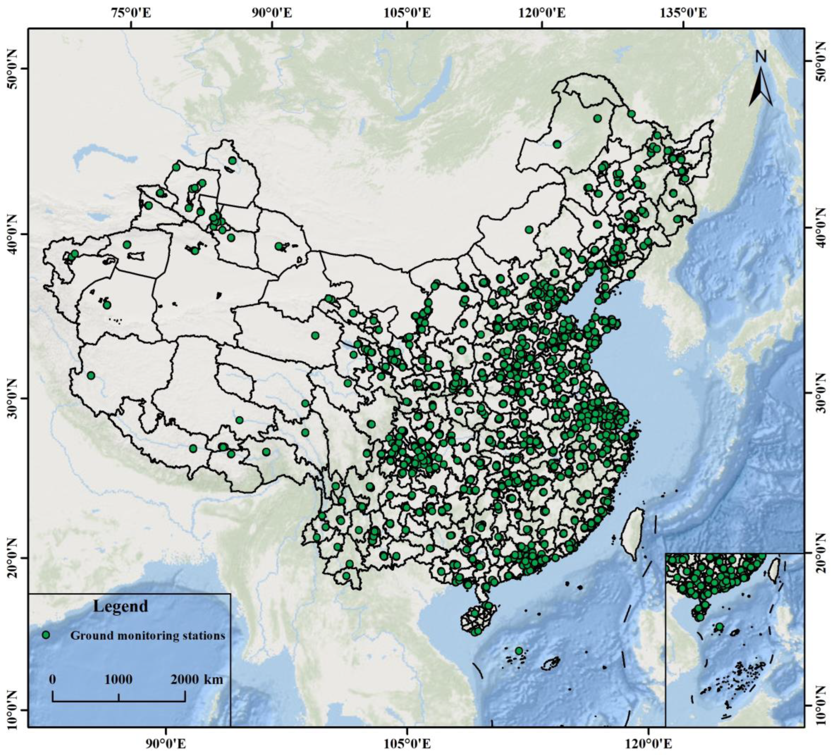
Due to factors such as satellite monitoring of atmospheric conditions and model estimation errors, the accuracy of remotely sensed PM2.5 concentration data (Dataset V5.GL.04) exhibits certain deviations compared to ground-based monitoring station measurements. Consequently, it is necessary to validate the accuracy of this dataset using ground station data. The ground station data employed in this study were obtained from the official website of the China National Environmental Monitoring Centre (CNEMC). These data comprise hourly PM2.5 concentration measurements from all stations across China for the period 2014–2021. As illustrated in Figure 1, the spatial distribution of monitoring stations is uneven, with a higher density observed in the eastern coastal regions and fewer stations distributed across the western areas.

Figure 1.
Spatial distribution of PM2.5 ground monitoring stations in China. Note: based on the standard map No. GS-0650 (2024) from the Standard Map Service website of the Ministry of Natural Resources, the base map boundaries remain unaltered. All subsequent maps use these boundaries as the standard reference.
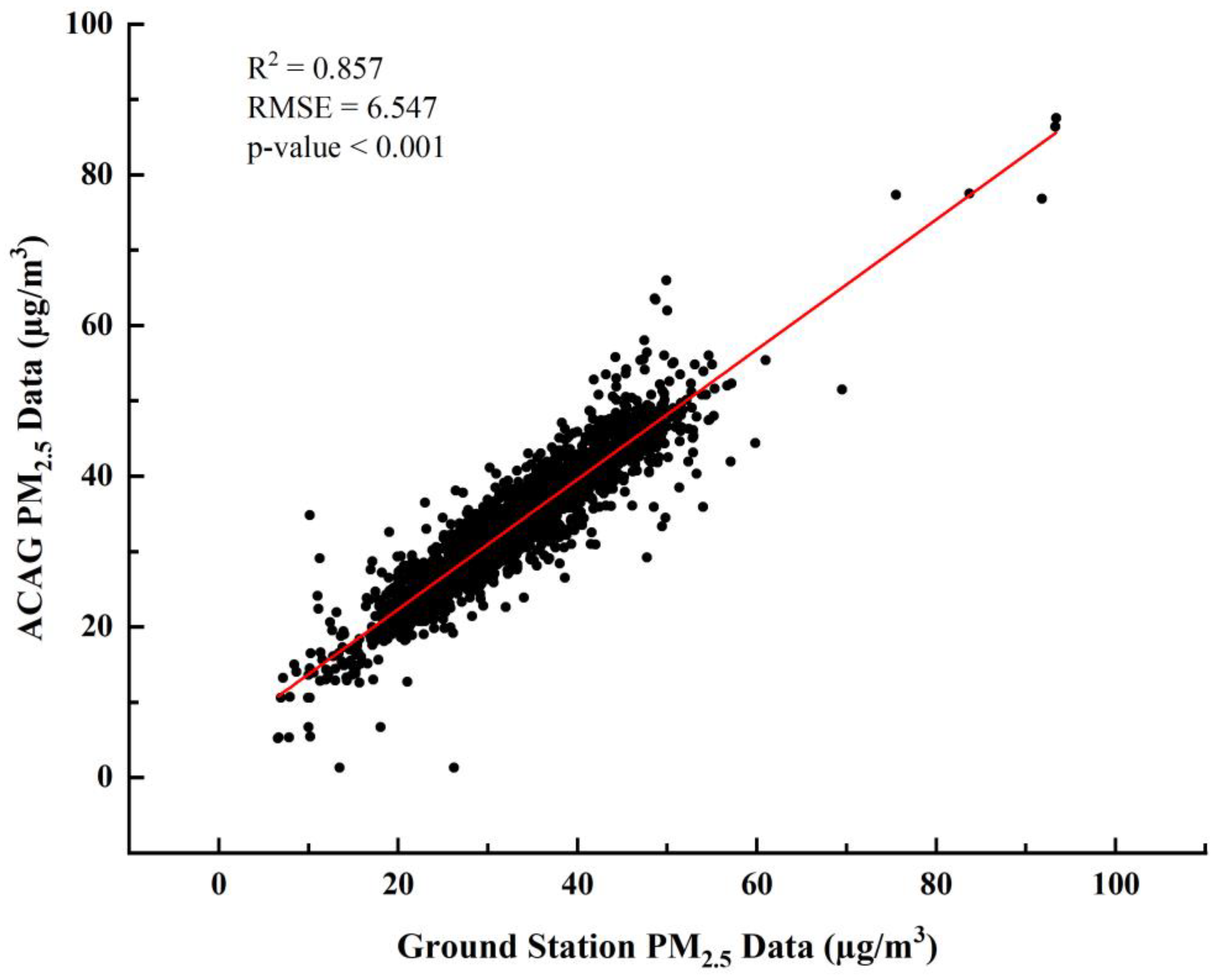
Utilizing the hourly PM2.5 concentration measurements from the monitoring stations, we computed the annual average PM2.5 concentration for each station using Python 3.11. Subsequently, a correlation analysis was performed between these ground-based station annual averages and the corresponding satellite-retrieved data (V5.GL.04). The results demonstrated a strong correlation, with an R2 of 0.857 and an RMSE of 6.547, and the analysis passed the significance test (Figure 2). This indicates that the satellite-retrieved dataset is suitable for subsequent analysis.
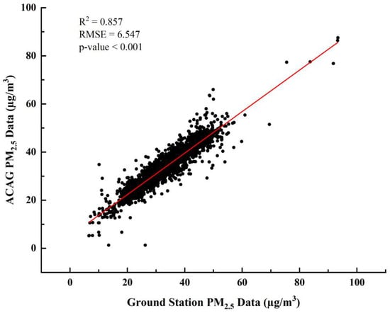
Figure 2.
Verification results of ground station PM2.5 and ACAG PM2.5.
2.1.3. Natural Environment Data
Natural environment data include annual precipitation (PRE), annual mean temperature (TEM), annual mean wind speed (WIN), annual mean relative humidity (RH), and vegetation coverage. The Normalized Difference Vegetation Index (NDVI), which effectively reflects the growth status of large-scale vegetation and serves as a robust indicator of vegetation coverage, was sourced from NASA’s regularly published MOD13A3 product with a spatial resolution of 1 km (https://earthdata.nasa.gov) (accessed on 20 January 2025). The NDVI gridded data underwent processing identical to the PM2.5 dataset: Zonal Statistics tool was applied to derive annual mean NDVI values for all cities. The remaining data were collected from China’s daily surface climate dataset (V3.0) released by the China Meteorological Administration (https://data.cma.cn) (accessed on 6 February 2025), which encompasses all meteorological stations across China. Using Python 3.11, we preprocessed the data to obtain annual averages for temperature, wind speed, and relative humidity at each station (while precipitation required summation), followed by spatial interpolation using the Inverse Distance Weighting (IDW) method at 1 km resolution. Finally, annual meteorological metrics for all cities were extracted based on vector boundaries.
2.1.4. Socioeconomic Data
Socioeconomic data specifically encompass per capita GDP (PGDP), industrialization level (IND) (the proportion of secondary sector), population density (PD), and energy consumption level (ECI). Among these, the PGDP, IND and PD were sourced from the China City Statistical Yearbook (2001–2022). Based on findings from Xiao et al. [50], night-time light data can accurately assess energy consumption in China. Due to the lack of long-term energy consumption data at the urban scale in existing statistics, this study converted the brightness of night-time lights into grayscale pixel values and summed these values within each city’s area to measure urban energy consumption [51]. The original night-time light data were obtained from the National Oceanic and Atmospheric Administration (NOAA) (http://www.ngdc.noaa.gov) (accessed on 18 February 2025).
Given the availability and completeness of socioeconomic data, this study employs panel data from 339 prefecture-level and above cities in China (excluding Hong Kong, Macau, and Taiwan) for spatial econometric analysis conducted using Stata 17. All variables were transformed using natural logarithms to maintain data consistency and lessen the impact of heteroscedasticity on the model results.
2.2. ESTDA
2.2.1. Global Spatial Autocorrelation
The application of spatial econometric models necessitates spatial correlation among the observations of the study units [52]. Consequently, this study utilized the global Moran’s I index to assess the spatial clustering of PM2.5:
where denotes the spatial weight matrix; indicates the average PM2.5 concentration across all cities; and and respectively, represent the PM2.5 values for cities i and j.
2.2.2. Local Indicators of Spatial Association (LISA) Time Path
LISA time path illustrates the paired movements of city units’ PM2.5 attribute values and their spatial lags, elucidating the local spatio-temporal interactions and dynamics of PM2.5 [26]. The movement path of LISA coordinates can be represented as , where denotes the standardized PM2.5 value for city i in year t, and indicates its spatial lag. The geometric characteristics include relative length (), tortuosity (), and movement direction (), expressed as follows:
where N is the number of cities, and T is the annual interval. The term represents the movement distance of city i from year t to year t + 1. indicates that the movement distance of city i’s LISA coordinates surpasses the average value, implying a dynamic local spatial structure in PM2.5 level growth. A larger value results in a more pronounced curvature of time path, indicating greater observed volatility in the evolution of the local spatial dependence associated with PM2.5 levels for city i. denotes the average annual movement direction for city i: directions from 0° to 90° (or 180° to 270°) indicate a synergistic high (or low) growth trend in PM2.5 levels for both the city and its surrounding regions; directions from 90° to 180° (or 270° to 360°) indicate a low (or high) growth trend locally, while neighboring areas experience high (or low) growth.
2.2.3. LISA Spatio-Temporal Transition
Based on the shifts in the types of local spatial associations of city units in Moran scatter plots over different periods, Rey and Janikas [25] proposed the theory of spatio-temporal transitions, categorizing them into four fundamental types depending on whether the spatial association type changed for the focal city unit itself (self), its neighboring units (neighbor), or both: type I (self-transition, neighbor stability) occurs when the focal unit transitions while its neighbors remain stable. Type II (self-stability, neighbor transition) describes stability in the focal unit’s type coupled with transitions in neighbor types. Type III (self-transition, neighbor transition) involves transitions in both the focal unit and neighbors. Type IIIA occurs when the transition directions of the focal unit and neighbors are consistent, whereas type IIIB features opposed transition directions between them. Type IV (self-stability, neighbor stability) represents full stability where both the focal unit and neighbors maintain their types. Detailed symbolic expressions are shown in Table S1. Moran scatter plot’s spatial stability is outlined below:
where represents the total cities that experienced type IV transitions during period t, and n is the total cities that could potentially undergo transitions.
2.3. Spatial Weight Matrix
Constructing a spatial weight matrix is a prerequisite and foundation for conducting spatial econometric analysis [53]. To mitigate model estimation errors from using a single spatial weight matrix, this study constructed and compared three matrices: the adjacency matrix (W1), the geographical distance matrix (W2), and the economic–geographical matrix (W3).
2.3.1. Adjacency Matrix (W1)
W1 primarily determines the spatial correlation between city units based on their spatial proximity. If two locations are adjacent, they are considered to have a correlation, with a weight of 1 assigned; if they are not adjacent, the weight is 0.
2.3.2. Geographical Distance Matrix (W2)
W2 is formed using the inverse of inter-city distances as weights. As the proximity between two locations enhances, the correlation intensifies, and the assigned weight becomes larger. The expression is as follows:
where denotes the distance separating city i from j.
2.3.3. Economic–Geographical Matrix (W3)
Building upon the geographical distance matrix, this study incorporated economic attributes to construct W3. The relevant expression is as follows:
where and , respectively, denote the mean GDP per capita for cities i and j during the study period.
2.4. Spatial Econometric Model
The spatial econometric model incorporates both spatial and temporal effects, effectively addressing the spatial dependence issues that traditional linear regression models cannot resolve, thereby ensuring that model specifications and estimation results more closely align with reality [54]. Common spatial econometric models encompass the spatial lag model (SLM), the spatial error model (SEM), and the spatial Durbin model (SDM). SLM addresses spatial dependence between a city’s dependent variable and those of its neighboring cities. SEM is applied when the spatial dependence manifests through the error term, while SDM accounts for spatial dependence in both the dependent and independent variables, making it more broadly applicable [55]. The expression for SDM used in this research is provided below:
where ρ and θ represent the regression coefficients of PM2.5 and explanatory variables, respectively, while β is the estimated parameter vector. and represent the space and time fixed effects. denotes a random error term. When θ = 0, SDM simplifies into SLM; when θ + ρβ = 0, it transforms into SEM [56].
2.5. GTWR
The GTWR investigates the spatio-temporal non-stationary relationships of regional variables by constructing locally dependent models. This approach is crucial for uncovering the local spatio-temporal variations in the factors influencing PM2.5. Its expression is as follows [43]:
where is the spatio-temporal coordinates of sample i, and and represent the regression coefficients and constant term, respectively. refers to the model’s error term. The calculation formula for the regression coefficient at sample i is as follows:
where indicates the spatio-temporal weight at sample i.
3. Results
3.1. Temporal Evolution of PM2.5
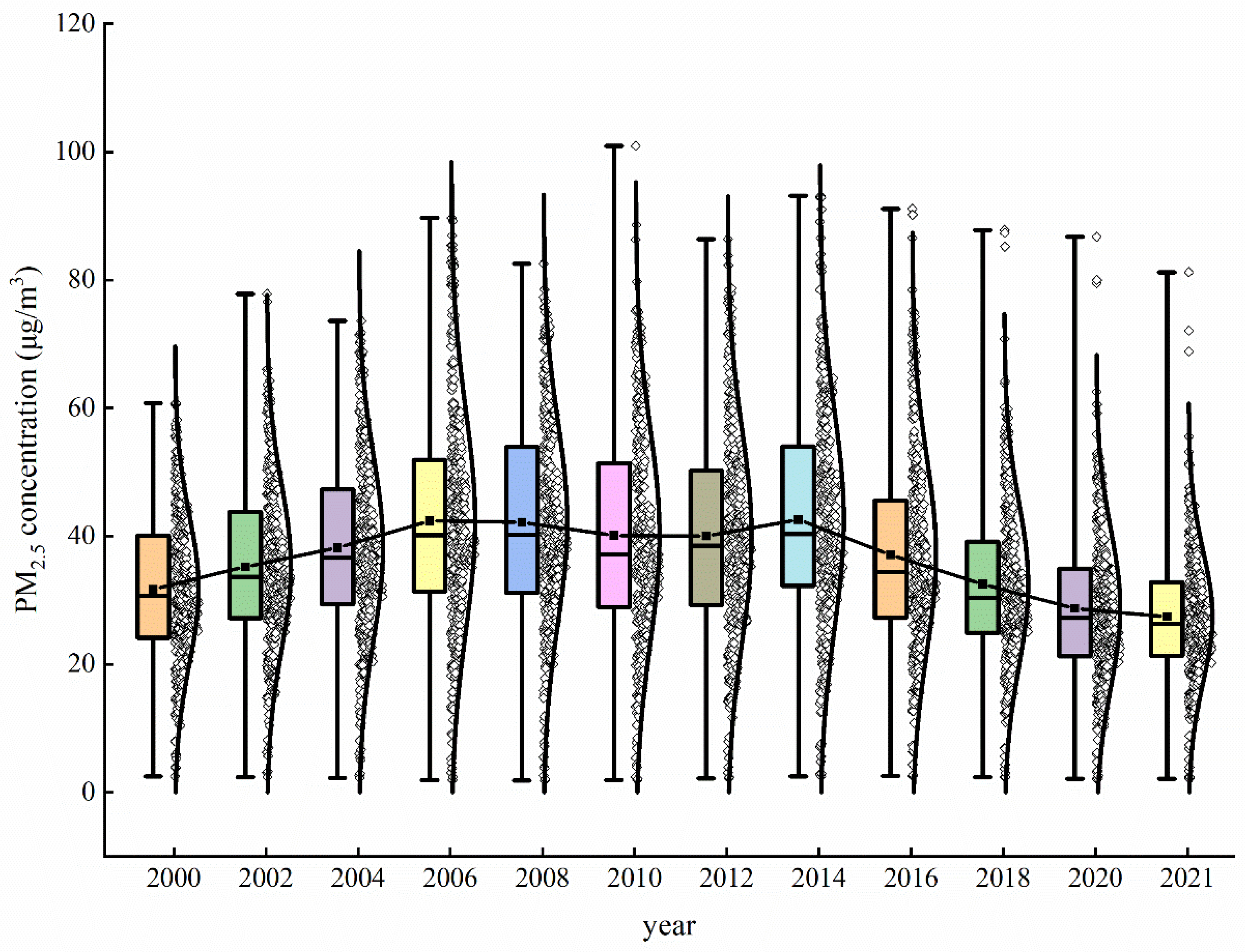
As illustrated in Figure 3, the PM2.5 concentration from 2000 to 2021 followed a trend consistent with a normal distribution, characterized by “bimodal” fluctuations and phased evolutionary patterns in the annual averages. However, significant variations were observed across different periods. From 2000 to 2007, China’s PM2.5 pollution levels continuously worsened, marked by a 35.02% increase in concentration. This phase was closely associated with the accelerated processes of industrialization and urbanization under the “Tenth Five-Year Plan” (2001–2005), during which rapid yet unregulated development resulted in ecological degradation and a marked decline in air quality [57]. For instance, energy-intensive industries such as steel and cement production expanded rapidly, contributing to a surge in coal consumption, while emission control technologies remained underdeveloped. Between 2007 and 2014, PM2.5 pollution did not improve, with a slight decline followed by a gradual intensification, peaking in 2014 at 42.6 µg/m3. This paradoxical trend can be attributed to two competing forces: (1) the 2008 global financial crisis temporarily reduced industrial output, leading to a short-term dip in PM2.5 emissions; and (2) China’s post-crisis economic stimulus package reignited energy-intensive sectors, particularly in the Beijing–Tianjin–Hebei (BTH), Yangtze River Delta (YRD), and Pearl River Delta (PRD) regions, where PM2.5 concentrations rebounded significantly due to intensified coal combustion and industrial activity [58]. From 2014 to 2021, a rapid decline in PM2.5 concentration occurred, dropping from 42.6 to 27.4 µg/m3. Evidently, 2014 marked a pivotal turning point in China’s PM2.5 pollution, with a transition from continuous deterioration to gradual improvement. This trend was primarily driven by stringent policy interventions but also influenced by extraordinary events such as the COVID-19 pandemic. In terms of regulatory efforts, the Chinese government enacted major air pollution control initiatives, including the “Air Pollution Prevention and Control Action Plan” and the “Three-Year Action Plan to Fight Air Pollution”, which contributed to a progressively notable improvement in PM2.5 pollution [59]. Simultaneously, the COVID-19 outbreak in late 2019 triggered unprecedented containment measures—including citywide lockdowns, the suspension of emission-intensive construction projects, the promotion of public transportation alternatives, and regulatory enforcement of emission reductions—which collectively enhanced air quality by suppressing anthropogenic emissions [60].
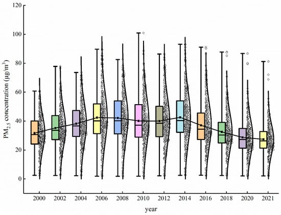
Figure 3.
Box plot and normal distribution of PM2.5 concentration trends in China. (The solid black rectangles within the boxes represent the annual average PM2.5 concentration across all cities, the whiskers indicate the range from minimum to maximum concentrations, and the hollow diamonds indicate the annual average PM2.5 concentration for individual cities.)
3.2. Spatial Distribution of PM2.5
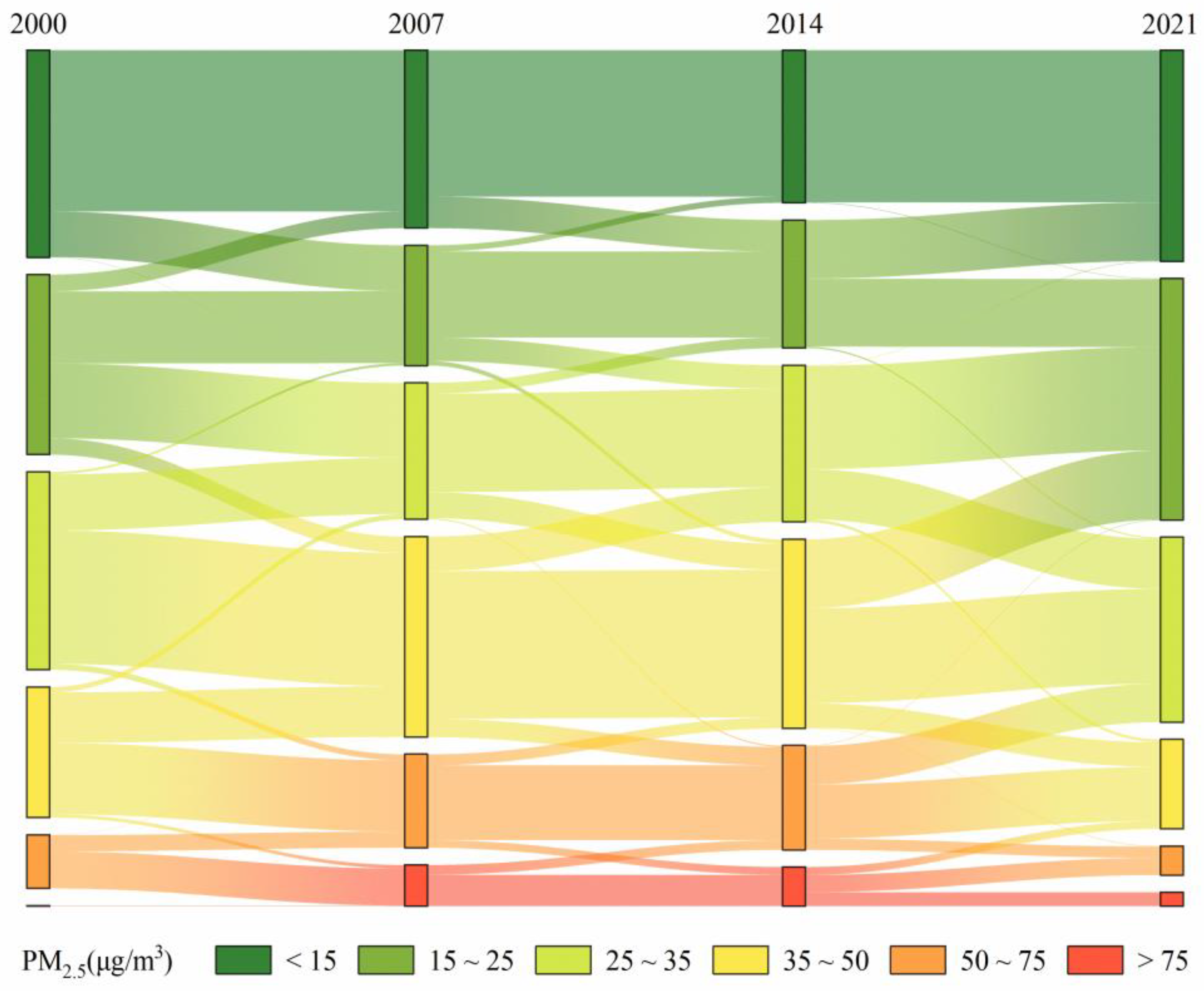
Based on the PM2.5 concentration limits established in Table S2, this study divided the concentrations into six intervals: <15 µg/m3, 15–25 µg/m3, 25–35 µg/m3, 35–50 µg/m3, 50–75 µg/m3, and >75 µg/m3 (Figure 4). From 2000 to 2021, the spatial variabilities in PM2.5 concentrations were significant, generally characterized by higher levels in the central and eastern regions as well as along the northwestern border, with lower levels in other areas. Specifically, (1) regions with low PM2.5 concentrations (<15 µg/m3) were primarily distributed across the Tibetan Plateau, the northern border of Xinjiang, and Eastern Inner Mongolia. These areas experience lower levels of human activity, slower economic development, and consequently fewer pollutant emissions, coupled with a strong ecological dilution capacity, resulting in well-preserved ecological environments and air quality [61]. (2) High-concentration PM2.5 areas (>50 µg/m3) demonstrated significant spatial clustering, with PM2.5 pollution gradually expanding from 2000 to 2014, until 2021, when China’s air quality showed marked improvement. (3) Throughout the study period, three major PM2.5 pollution centers were identified: the Beijing–Tianjin–Hebei urban agglomeration, the Yangtze River Delta urban cluster, and the Taklamakan Desert region, likely influenced by population density, economic development, and the unique climatic conditions of the desert [62,63].
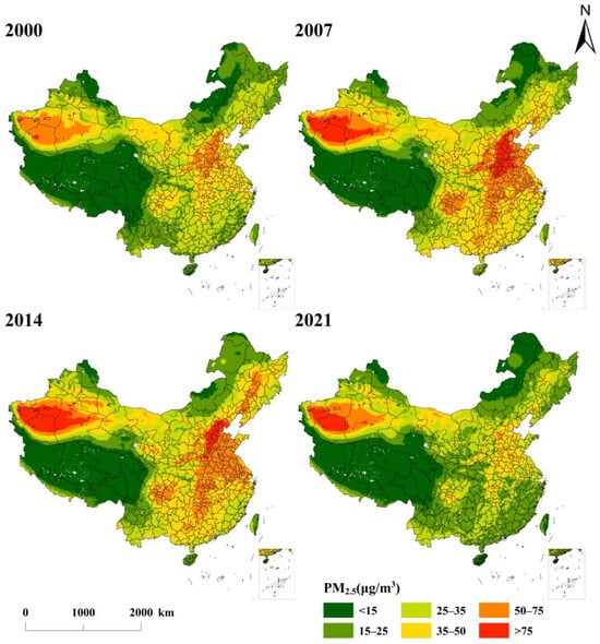
Figure 4.
Spatial distribution of interannual PM2.5 concentrations in China.
It is noteworthy that Figure 5 reveals that the evolution in PM2.5 concentration types predominantly occurs through successive transitions between adjacent categories, with cross-level transitions being less likely. This observation indirectly reflects that mitigating PM2.5 pollution is a continuous and gradual process, making it challenging to fully reverse the severe air pollution situation in a short period [64].
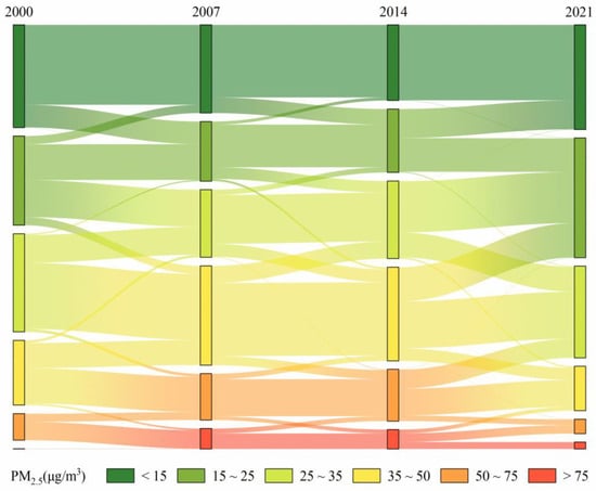
Figure 5.
Sankey diagram of PM2.5 concentration type transfer matrix.
3.3. Local Spatio-Temporal Dependence of PM2.5
3.3.1. Relative Length and Tortuosity
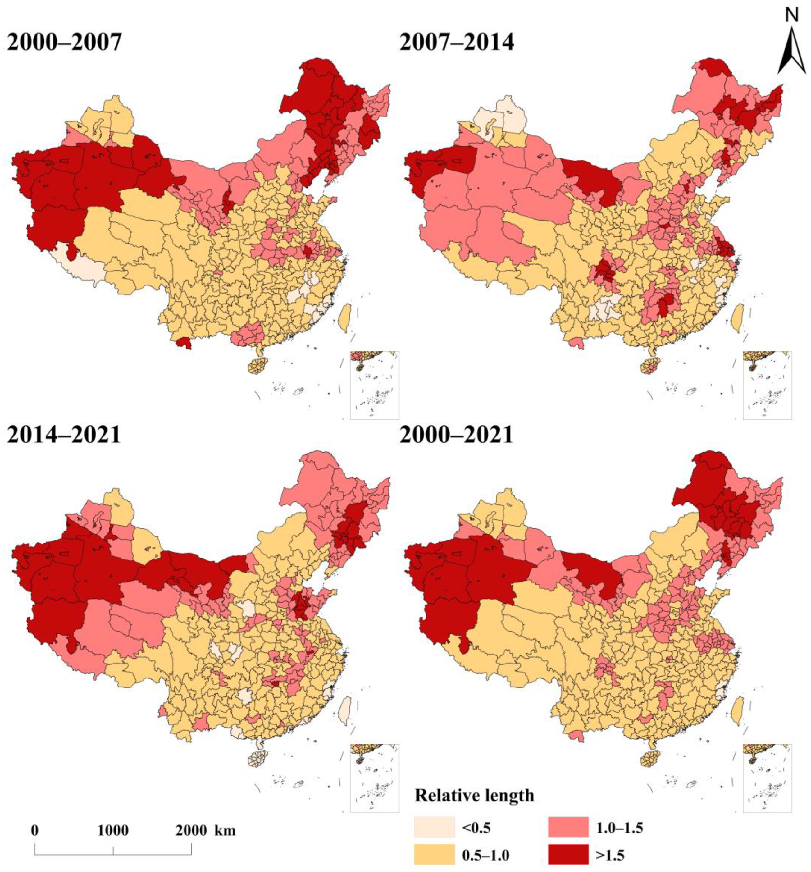
The geometric features of the LISA time path are utilized to delineate the local structure and spatio-temporal dependencies of PM2.5 pollution. As depicted in Figure 6, from 2000 to 2007, 130 cities exhibited a relative length exceeding 1, representing 34.9% of the total. This figure increased to 156 cities between 2007 and 2014, predominantly concentrated in northern regions, signaling a robust dynamic local spatial structure in PM2.5 concentration growth. However, from 2014 to 2021, the number of cities with a relative length greater than 1 declined. Apart from spatial clustering observed in the Northeast, Northwest, and Shandong Peninsula, the spatial structure of pollution in other regions remained relatively stable. Overall, the local spatial dynamics of PM2.5 pollution in Northern China from 2000 to 2021 were generally more prominent than in southern regions, particularly in the three northeastern provinces, the Northwest, and cities across the North China Plain. In the South, the most significant impacts were observed in the middle and lower reaches of the Yangtze River. This spatial disparity can be attributed to regional development patterns and the implementation of national strategies. In Northern China, greater reliance on coal-based energy systems for industrial production and winter heating, combined with the persistence of traditional energy-intensive industries, has delayed the transition to cleaner production modes, thereby amplifying pollution fluctuations. Concurrently, the execution of national strategies, such as the Northeast Revitalization, Western Development, and Rise of Central China, has reinforced traditional industrial structures, exacerbating environmental pollution during economic development [65]. In contrast, southern regions underwent earlier industrial upgrading and accelerated renewable energy deployment, resulting in more stable environmental dynamics.

Figure 6.
Distribution of relative length of PM2.5 concentration at different stages in China.
Throughout the study period, the tortuosity values consistently remained above 1 (Figure 7), underscoring weak stability in the spatial dependence direction of PM2.5. Spatially, the number of cities with a tortuosity exceeding 14.2 increased progressively across the three phases, with varying coverage areas. This trend was particularly evident in regions with intensive economic activity and higher levels of industrialization, where the volatility of spatial dependence in PM2.5 pollution became more pronounced. Notably, Guangxi and Hainan exhibited distinct tortuosity shifts driven by interacting monsoonal and socioeconomic forces. Seasonal reversals in the South China Sea monsoon created opposing pollution pathways: winter northeasterlies transported Pearl River Delta emissions to Guangxi, while summer southwesterlies enhanced atmospheric cleansing over Hainan. Meanwhile, asymmetric development pacing amplified differences: Guangxi’s accelerated industrial restructuring disrupted established pollution networks, whereas Hainan’s post-2018 pivot to tourism-dominated economies decoupled its PM2.5 dynamics from mainland industrial cycles. These interacting mechanisms resulted in higher spatio-temporal volatility than that observed in inland regions.
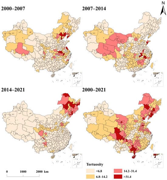
Figure 7.
Distribution of tortuosity of PM2.5 concentration at different stages in China.
3.3.2. Movement Direction
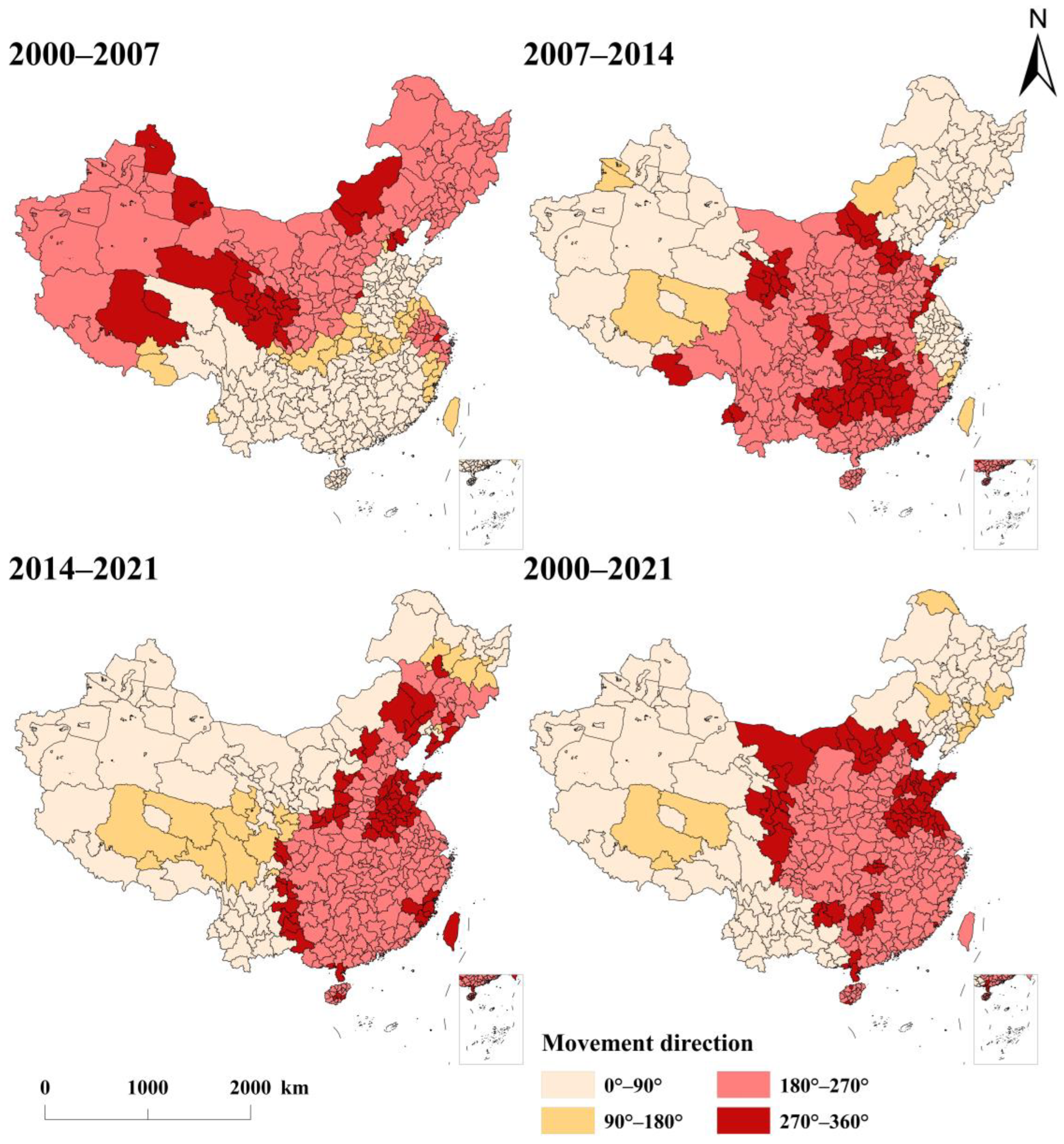
The spatial integration characteristics of changes in PM2.5 pollution are effectively revealed by the movement direction within the geometric parameters of the LISA time path (Figure 8). From 2000 to 2007, 313 cities experienced either synergistic high growth or synergistic low growth in PM2.5 levels, representing 84.1% of the total. This highlights a strong spatial integration in the evolution of PM2.5 pollution. However, the pattern of the PM2.5 movement direction from 2007 to 2014 diverged significantly from the first phase. Cities with synergistic high-growth trends began to shift toward the northeastern and northwestern regions, while synergistic low-growth trends gradually migrated to the southern regions. Throughout this phase, the count of cities experiencing synergistic growth decreased to 291, reflecting a weakening trend in the spatial integration of PM2.5 pollution evolution. During the third phase, cities with synergistic high growth were mainly situated west of the Hu Line, likely due to inadequate environmental protection awareness in the western regions as industrialization and urbanization accelerated, leading to increased PM2.5 pollution [66]. On the whole, changes in PM2.5 pollution in China were primarily marked by synergistic growth, accompanied by spatial integration features where both synergy and competition coexisted.

Figure 8.
Distribution of PM2.5 concentration movement direction at different stages in China.
3.4. Spatio-Temporal Transition
The transition of local spatial correlation categories of PM2.5 pollution is effectively captured by the spatio-temporal transfer probability matrix. As shown in Table 1, the values located off-diagonal are consistently smaller than those found on the diagonal, with the minimum diagonal value being 0.587. This indicates that a city’s PM2.5 transition type is at least 58.7% likely to remain unchanged in the following periods, a rate notably greater than transitioning to other types. Specifically, the highest transfer probability from 2000 to 2007 was HLt → LLt+1 (0.265), with 27 cities undergoing this transition. Notably, this transition continued to have the highest probability in the following two periods, involving 35 and 30 cities, respectively, while other types exhibited lower transfer probabilities. The observed persistence primarily stems from three interdependent constraints: First, established industrial systems resist transformation due to high retrofit costs, perpetuating emission-intensive activities in manufacturing hubs and maintaining spatial stability. Second, policy implementation delays prolong transition periods for industrial cities shifting from pollution-intensive modes, resulting in execution gaps for emission reduction targets. Third, stable labor forces in traditional industrial regions reinforce existing production networks, constraining rapid spatial reorganization. Collectively, these structural, governance, and socioeconomic barriers contribute to the lock-in of PM2.5 pollution patterns. Overall, type IV transitions were the most prevalent, occurring in 89.6% of cities. This suggests a strong path dependence in the spatial clustering of PM2.5, largely attributed to the long-term processes of industrialization and economic growth, which make it challenging to reduce pollution levels in the short term [57]. The transition proportions for types I, II, and III were 0.064, 0.033, and 0.008, respectively, indicating that a city’s PM2.5 levels are more influenced by internal factors than by spillover effects from neighboring units.

Table 1.
Spatio-temporal transitions and probability matrices of PM2.5 in different stages.
3.5. Analysis of Factors Influencing PM2.5
3.5.1. Preprocessing of Independent Variables
To mitigate the potential instability in model construction caused by multicollinearity among variables, a variance inflation factor (VIF) analysis was conducted on the selected variables. The results showed that all VIF values were less than 10, indicating no multicollinearity (Table 2).
Table 2.
Descriptive statistics and VIF test results of independent variables.
3.5.2. Test Results of Model Selection
As shown in Table S3, PM2.5 in China exhibits significant spatial autocorrelation, indicating spatial interactions between cities. Consequently, incorporating geographical spatial factors into the analytical framework for PM2.5 pollution determinants is necessary.
A stepwise testing approach was employed to identify the optimal spatial econometric model. All test statistics were statistically significant at the 1% level; therefore, the diagnostic analysis in the model selection section uses the W1 test results as an illustrative example, with analyses for W2 and W3 showing similar statistical characteristics. The diagnostic procedure commenced with Lagrange Multiplier (LM) and Robust Lagrange Multiplier (LM) tests to evaluate spatial dependence nature. The LM-lag test and LM-error test both yielded statistically significant results (LM-lag = 1551.17, p < 0.001; LM-error = 4738.45, p < 0.001 in Table 3), indicating spatial autocorrelation exists. Given the simultaneous significance of both baseline LM tests indicating possible interference between dependence types, Robust LM tests were implemented to conduct conditional hypothesis testing: Robust LM-lag test (controlling for error dependence) yielded a statistic of 269.74 (p < 0.001), while Robust LM-error test (controlling for lag dependence) produced a statistic of 3457.02 (p < 0.001). The simultaneous significance of both Robust LM tests confirms dual spatial dependence—evidenced by substantive spillovers in the dependent variable and spatial autocorrelation in unobserved factors. This indicates that the SDM should be estimated as the initial model choice. Subsequent Wald and Likelihood Ratio (LR) tests evaluated whether the SDM could simplify to SLM or SEM, with comprehensive results from Table 3 confirming SDM’s necessity: The Wald-lag test (statistic = 119.42, p < 0.001) and LR-lag test (statistic = 120.48, p < 0.001) jointly rejected SLM simplification, while the Wald-err test (statistic = 149.85, p < 0.001) and LR-err test (statistic = 40.87, p < 0.001) collectively refuted SEM simplification, all at a 1% significance level. The consistent results across both Wald and LR tests for both simplification paths (to SLM and SEM) definitively established SDM’s irreducibility, validating its selection as the comprehensive framework. Concurrently, the Hausman test (statistic = 124.18, p < 0.001) resolved the fixed versus random effects dilemma by detecting a significant correlation between unobserved individual effects and regressors, confirming fixed effects superiority for consistent estimation. Finally, LR tests for fixed effects types assessed spatio-temporal heterogeneity, with the test for spatial fixed effects yielding a statistic of 67.59 (p < 0.001) and the time fixed effects test producing a statistic of 10,427.39 (p < 0.001). Both results were statistically significant at the 1% level, indicating the superiority of the spatio-temporal double fixed effects model.
Table 3.
Test results of the spatial econometric model under three spatial weight matrices.
This diagnostic sequence—comprising confirmation of dual spatial dependence (lag and error) via LM and Robust LM tests, verification of the SDM’s irreducibility through Wald and LR tests, selection of fixed effects using Hausman test, and assessment of spatio-temporal heterogeneity with LR tests—collectively supported our final SDM with spatio-temporal double fixed effects to elucidate the spatial spillover effects related to PM2.5.
3.5.3. Estimated Results of SDM
Table 4 demonstrates that the adjusted R2 values for all models exceed 0.635, and the regression coefficients for independent variables across the three spatial weight matrices are consistent in direction and significance. This consistency highlights the strong fit and robustness of the SDM. Furthermore, the significant spatial autoregression coefficient (ρ) at the 1% level in the SDM indicates a notable positive spatial spillover effect for China’s PM2.5 pollution. Controlling for other variables, a 1% variation in PM2.5 concentration in nearby cities is anticipated to cause at least a 0.981% variation in local PM2.5 levels. Specifically, precipitation, temperature, wind speed, and NDVI negatively impact PM2.5 pollution, while relative humidity, per capita GDP, industrialization level, and energy consumption exert a significant positive influence. These findings align with the majority of scholarly studies [67,68]. Notably, the quadratic term of log-transformed per capita GDP is significantly negative, indicating a reverse “U”-shaped correlation linking economic development to PM2.5 pollution, thereby supporting the EKC hypothesis. The influence of population density on the spatial variation of PM2.5 is less pronounced. Despite some debate, it generally exhibits a positive correlation [69]. In terms of spatial lag effects, increases in local precipitation, wind speed, NDVI, and energy consumption mitigate PM2.5 pollution in neighboring cities, while increases in temperature and per capita GDP exacerbate it.
Table 4.
Estimation results of the SDM under three spatial weight matrices.
3.5.4. Decomposition of Spatial Effects
Due to the existence of spatial spillover effects, the estimation results in Table 4 cannot accurately capture the marginal impacts of each variable on PM2.5 pollution [70]. Consequently, further analysis of the direct and indirect effects of these factors is necessary (Table 5). Notably, since the log L and adjusted R2 values of the W3 model in Table 4 are higher than those of the W1 and W2 models, the subsequent analysis will be grounded in the W3 model.
Table 5.
Estimation results of direct and indirect effects under W3.
Among natural environmental factors, a significantly negative direct effect coefficient is associated with precipitation, while its indirect effect is insignificant, indicating that PM2.5 pollution is effectively suppressed locally by precipitation. Theoretically, during precipitation, raindrops capture PM2.5 particles from the air and deposit them on the ground, thereby reducing PM2.5 concentrations [71]. Conversely, relative humidity demonstrates a significant positive direct effect, as higher humidity promotes the hygroscopic growth of aerosols or accelerates the secondary formation of nitrates and sulfates, leading to increased PM2.5 concentrations [72]. However, studies have also suggested that when relative humidity exceeds a certain threshold, PM2.5 may aggregate and be reduced through wet deposition (precipitation) [73]. The direct effect of temperature also shows a negative impact and passes the significance test at the 1% level, likely because high temperatures increase the evaporation loss of PM2.5, including the loss of ammonium nitrate and other volatile or semi-volatile components, leading to reduced concentrations [74]. Nevertheless, the indirect effect of temperature exhibits a significantly positive impact, mainly attributed to the fact that high temperatures promote atmospheric convection, accelerating the transport of volatile or semi-volatile components to neighboring regions while simultaneously promoting photochemical reactions during transport that generate more PM2.5 precursors, resulting in increased concentrations [75]. Essentially, this represents a spatial redistribution of pollution rather than its elimination. Wind speed exerts a significantly negative direct effect. This indicates that increased wind speed generally creates favorable conditions for the dispersion of PM2.5, effectively reducing concentrations locally [68]. However, the positive indirect effect of wind speed suggests that it facilitates the cross-regional transport of PM2.5 by enhancing atmospheric mobility, consequently increasing PM2.5 concentrations in neighboring cities. The enhancement of vegetation coverage was found to effectively mitigate PM2.5 pollution, mainly attributed to the fact that vegetation not only physically adsorbs PM2.5 but also impedes its movement [76], thereby filtering and purifying the air on a regional scale. Thus, increasing vegetation coverage and optimizing ecosystem management are considered effective strategies for controlling PM2.5 pollution.
Among socioeconomic factors, increases in per capita GDP and industrialization levels are found to exacerbate PM2.5 pollution in local cities, primarily because economic growth is often accompanied by increased industrial production, transportation, and other human activities that emit large quantities of air pollutants [77]. The significant indirect effect of per capita GDP may be attributed to the diffusion of technology and spillover effects from local economic development, potentially reducing pollution levels in nearby cities. Additionally, the direct effect of the quadratic term of log-transformed per capita GDP is significantly negative. This suggests that while initial economic development may increase PM2.5 pollution, continued growth beyond a certain environmental threshold leads to improved air quality [45]. The direct effect of energy consumption is similarly aligned with per capita GDP and industrialization levels. Given that electricity production in China remains predominantly coal-based, the combustion of large amounts of fossil fuels contributes to increased PM2.5 emissions [67]. Nevertheless, its indirect effect shows a negative impact, possibly because the increased use of clean energy in local cities has encouraged neighboring cities to adopt similar environmental protection measures.
3.5.5. Estimated Results of GTWR
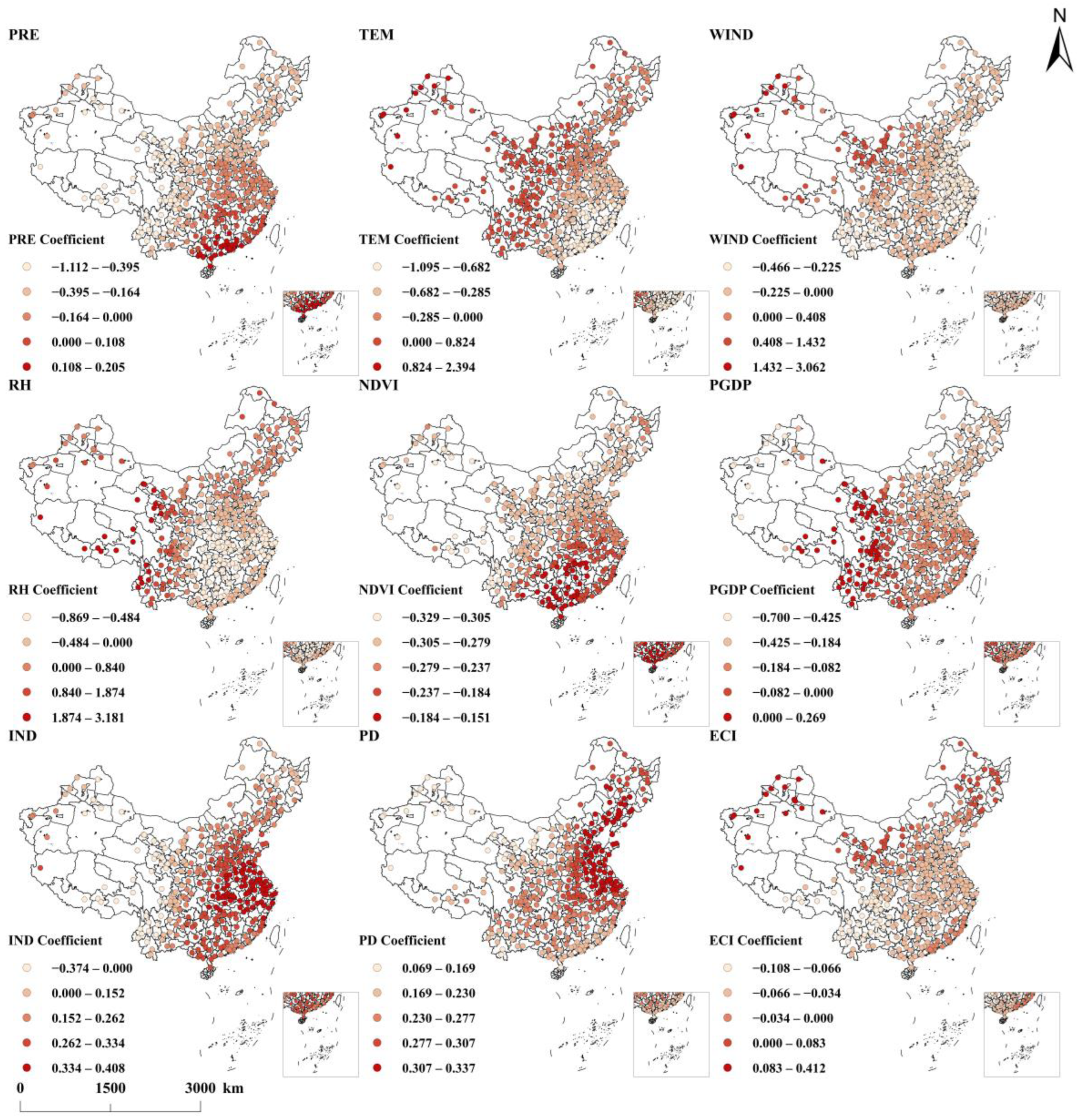
The GTWR model effectively reveals the local spatio-temporal variations in PM2.5 concentrations, influenced by different natural environmental factors and socioeconomic activities (Figure 9). As shown in Table 6, the model demonstrates strong robustness, with an adjusted R2 of 0.860.
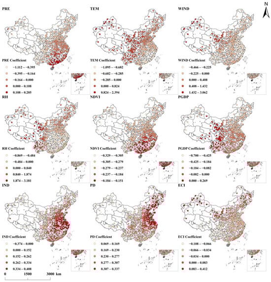
Figure 9.
Distribution of regression coefficients for independent variables.
Table 6.
Estimated parameters of GTWR.
The impact of precipitation on PM2.5 is predominantly negative, yet a positive correlation is observed in Southern China. This apparent anomaly stems from the region’s unique climate and chemical feedback mechanisms: the vast majority of rainfall in South China consists of light precipitation with limited scavenging efficiency, which cannot effectively remove PM2.5. Conversely, light precipitation and rain–fog processes increase atmospheric humidity, promoting nitrate-dominated hygroscopic growth and consequently leading to higher PM2.5 concentrations [78]. Furthermore, substantial ammonia emissions from intensive agriculture react with accumulated nitrate/sulfate during prolonged overcast and rainy conditions, generating secondary inorganic aerosols that offset wet deposition losses. Relative humidity exerts a negative influence in Southern China. Due to a threshold effect in the direction of relative humidity’s impact on PM2.5 concentration, when relative humidity exceeds this threshold (usually 80% [78]), increased humidity causes suspended particles to coagulate and increase their weight, thereby accelerating the sedimentation rate of PM2.5 and resulting in a significant reduction in its concentration [73]. Temperature and wind speed exhibit negative correlations with PM2.5 along the eastern coastal areas, which is closely related to the region’s flat topography and open marine environment. Conversely, in the northwestern inland areas, low temperatures and the complex terrain of mountains and basins restrict air circulation, causing pollutants to accumulate [2]. Enhanced vegetation coverage significantly reduces PM2.5 concentrations, as confirmed by the results of spatial econometric regression. The correlation linking per capita GDP to PM2.5 varies significantly across regions. In the more economically developed eastern regions, the environmental pollution inflection point has evidently been surpassed, whereas in the underdeveloped western regions, economic growth still comes at the cost of the environment [66]. Furthermore, with adjustments in the energy consumption structure and a growing share of renewable sources, atmospheric pollutants in the eastern regions are gradually decreasing [79]. Industrialization levels and population density generally exhibit a positive correlation with PM2.5, aligning with existing research findings [67].
4. Discussion
In the study of spatio-temporal patterns of PM2.5, Ali et al. [80] investigated pollution hotspots and trends in China from 2001 to 2020. This study aligns closely with Ali et al.’s core finding that 2014 is identified by both as a pivotal turning point for PM2.5 pollution. However, a significant divergence exists in their periodization schemes: our research employs a more granular three-phase analysis (rising–fluctuating–declining), revealing a localized decrease in PM2.5 levels around 2007, whereas Ali et al., based on provincial-scale data, indicate a general upward trend in PM2.5 concentrations across most Chinese provinces from 2001 to 2012. Both studies attribute the post-2014 improvements to the “Air Pollution Prevention and Control Action Plan” and the “Three-Year Action Plan to Fight Air Pollution”, but this study further highlights the impact of COVID-19 containment measures. Regarding spatial distribution, the two studies show both consensus and key differences in identifying pollution hotspots. The primary consensus lies in their joint identification of the North China Plain and the Taklamakan Desert in Northwest China as core pollution zones, and the Tibetan Plateau and Northeast China as clean areas. A critical difference is that this study additionally identifies the Yangtze River Delta urban agglomeration as a pollution center, while Ali et al.’s provincial-level analysis emphasizes central Henan–Hubei and the Sichuan Basin. Qi et al. [51] similarly explored the spatio-temporal evolution of PM2.5 concentrations across different climatic zones in China from 2000 to 2018, highlighting the Beijing–Tianjin–Hebei region, Shandong Peninsula, Sichuan Basin, and Xinjiang as high-concentration clusters. However, due to this study’s longer timeframe and evidence from 2021 spatial distribution data showing significant air quality improvements in the Shandong Peninsula and Sichuan Basin, these areas were not classified as persistent PM2.5 pollution hotspots in our analysis. Furthermore, Qi et al. quantified spatial dynamics using a standard deviational ellipse, revealing a long-term stagnation of the PM2.5 centroid around Nanyang City in Henan Province and an increasingly dispersed pollution pattern—aspects not addressed in the current study.
Regarding the factors influencing PM2.5, Cheng et al. [67] employed a spatial panel model to empirically analyze the key drivers of PM2.5 pollution across 285 Chinese cities. Their results indicate significant global spatial autocorrelation and local spatial clustering in urban haze pollution in China, along with a pronounced inverted U-shaped curve relationship between economic development level and air pollution—findings highly consistent with the conclusions of the present study. Furthermore, while Cheng et al. primarily focused on socioeconomic factors affecting PM2.5, this study provides a more comprehensive examination encompassing both natural environmental and socioeconomic factors. We also introduce GTWR to further elucidate the local spatio-temporal heterogeneity in the magnitude of influence exerted by various factors on PM2.5. Nevertheless, notable similarities exist, as both studies confirm that economic development level, energy intensity, and industrial structure exert a significantly positive influence on PM2.5 concentrations. Wang et al. [81] utilized GWR to explore the strength and direction of associations between various factors and PM2.5 in Chinese cities, incorporating landscape factors—an aspect not explicitly addressed in the current study. While GWR captures spatial non-stationarity in PM2.5 relationships by constructing spatially dependent local models, it neglects temporal non-stationarity and thus inadequately explains the spatio-temporal dynamics between influencing factors and PM2.5. Additionally, Wang et al. overlooked the spatial spillover effects of PM2.5, considering only the local-scale mechanisms of influence and consequently failing to account for cross-regional air pollution issues.
Finally, from a methodological perspective, the ESTDA framework places greater emphasis on the continuity of PM2.5’s temporal evolution and spatial patterns, thereby enabling a more efficient investigation of its spatio-temporal coupling mechanisms. It is noteworthy that this study addresses the estimation bias inherent in traditional models—caused by neglecting the spatial dependence of PM2.5—through the construction of a spatial econometric model focused specifically on China’s prefecture-level and above cities. This approach better explains cross-regional PM2.5 pollution issues, and the simulation results demonstrate high validation accuracy. Furthermore, this study incorporates the spatio-temporal heterogeneity of natural environmental and socioeconomic factors from a local perspective, thereby compensating for the common oversight of spatio-temporal heterogeneity in regression parameters across regions within spatial econometric models. The empirical analysis of PM2.5 across China’s prefecture-level and above cities further demonstrates that the combined application of ESTDA, spatial econometric modeling, and GTWR facilitates an in-depth exploration of PM2.5’s spatio-temporal dynamics, including the underlying spatial spillover effects of contributing factors and their local spatio-temporal variations.
5. Conclusions and Policy Implications
This study employed the ESTDA framework to comprehensively characterize the spatio-temporal patterns of PM2.5 pollution in China. Additionally, three spatial weight matrices were constructed, and influencing factors were quantitatively evaluated using SDM and GTWR models. The key findings are as follows. (1) From 2000 to 2021, PM2.5 concentrations exhibited a “bimodal” variation pattern and phased evolutionary characteristics. Spatially, three major PM2.5 pollution centers were identified. (2) The local spatial clustering of PM2.5 indicated strong path dependence, with transitions across different types displaying significant inertia. (3) A notable positive spatial spillover effect of PM2.5 pollution was observed. Natural environmental and socioeconomic factors exhibited distinct local spatio-temporal variations.
Drawing from the empirical results, relevant policy recommendations are proposed. (1) A collaborative regional strategy to prevent and control PM2.5 pollution needs to be implemented. Based on the spatio-temporal evolution patterns of PM2.5, the most severely affected areas are primarily concentrated in the Beijing–Tianjin–Hebei urban agglomeration, the middle and lower reaches of the Yangtze River, and the Taklamakan Desert region. Consequently, PM2.5 mitigation efforts in China should prioritize these three high-pollution areas by establishing an interconnected environmental monitoring network among regions to achieve coordinated control and joint management of PM2.5 pollution. (2) Transform the economic growth model and elevate the green development level. By quantifying the correlation linking per capita GDP to PM2.5, this study reveals that the win–win scenario of economic growth and environmental quality has not yet been fully realized. As China is currently undergoing a critical transition toward high-quality green development, it is essential that new development concepts be integrated across all sectors, accelerating the shift in the economic growth model towards sustainable development. Building on the identified PM2.5 pollution centers, targeted strategies should be deployed: For the Beijing–Tianjin–Hebei region, accelerating ultra-low emission retrofits in steel and cement clusters through green manufacturing subsidies should be prioritized, coupled with expanding hydrogen-powered public transport networks to phase out diesel fleets. In the Yangtze River Delta, integrated green port initiatives—including shore power infrastructure for berthed vessels—must advance alongside shared emission reduction platforms across electronics and textile industrial parks to enable multi-pollutant co-control. Meanwhile, Northwest China requires the deployment of subsidized solar-powered heating systems in oasis cities alongside cross-provincial desertification barriers to mitigate dust emissions. (3) Optimize industrial structure and enhance energy efficiency. The primary contributors to PM2.5 pollution are industrial production and energy consumption. Therefore, efforts should be directed toward developing emerging industries and modern service sectors to facilitate industrial restructuring. Additionally, the development and utilization of clean and renewable energy should be actively promoted to reduce reliance on fossil fuels. To achieve this, it is essential to advance region-specific industrial and energy transitions based on dominant pollution sources. For the Beijing–Tianjin–Hebei region, a shift should be made toward green manufacturing in key industries like steel production through government-backed technology upgrades while promoting electric vehicles in freight transport networks. In the Yangtze River Delta, it is important to foster cross-industrial resource-sharing platforms among manufacturing parks to reuse materials and energy, as well as expand renewable-powered logistics hubs in port areas. For Northwest China, solar energy projects should be integrated with desert control initiatives by installing photovoltaic systems on restored lands while subsidizing clean heating alternatives in urban communities.
Supplementary Materials
The following supporting information can be downloaded at: https://www.mdpi.com/article/10.3390/rs17132212/s1, Table S1: The categories of spatio-temporal transitions; Table S2: Standard values of PM2.5 concentration (µg/m3) established by the WHO and China; Table S3: Global Moran’s index for PM2.5 under three spatial weight matrices.
Author Contributions
Conceptualization, L.C. and Y.N.; methodology, L.C. and M.C.; software, L.C.; validation, L.C. and C.W.; formal analysis, L.C.; investigation, L.C. and H.W.; data curation, L.C. and C.W.; writing—original draft preparation, L.C.; writing—review and editing, L.C. and Y.N.; visualization, L.C. and H.W.; project administration, Y.N.; funding acquisition, Y.N. All authors have read and agreed to the published version of the manuscript.
Funding
This research was funded by the Central Guidance for Local Science and Technology Development Fund Program (Grant No. 25ZYJA019) and the National Tibetan Plateau Data Center (TPDC), Beijing 100101, China.
Data Availability Statement
No new data were created or analyzed in this study.
Conflicts of Interest
The authors declare no conflicts of interest.
References
- Geng, G.; Zheng, Y.; Zhang, Q.; Xue, T.; Zhao, H.; Tong, D.; Zheng, B.; Li, M.; Liu, F.; Hong, C.; et al. Drivers of PM2.5 Air Pollution Deaths in China 2002–2017. Nat. Geosci. 2021, 14, 645–650. [Google Scholar] [CrossRef]
- Xia, S.; Liu, X.; Liu, Q.; Zhou, Y.; Yang, Y. Heterogeneity and the Determinants of PM2.5 in the Yangtze River Economic Belt. Sci. Rep. 2022, 12, 4189. [Google Scholar] [CrossRef] [PubMed]
- Ulpiani, G. On the Linkage between Urban Heat Island and Urban Pollution Island: Three-Decade Literature Review towards a Conceptual Framework. Sci. Total Environ. 2021, 751, 141727. [Google Scholar] [CrossRef]
- Liu, Q.; Son, Y.J.; Li, L.; Wood, N.; Senerat, A.M.; Pantelic, J. Healthy Home Interventions: Distribution of PM2.5 Emitted during Cooking in Residential Settings. Build. Environ. 2022, 207, 108448. [Google Scholar] [CrossRef]
- Zaini, N.; Ean, L.W.; Ahmed, A.N.; Abdul Malek, M.; Chow, M.F. PM2.5 Forecasting for an Urban Area Based on Deep Learning and Decomposition Method. Sci. Rep. 2022, 12, 17565. [Google Scholar] [CrossRef]
- Wang, N.; Zhou, L.; Liu, L.; Song, T.; Luo, Q.; Li, Y.; Yang, F. Chemical Characteristics and Formation Mechanisms of PM2.5 during Wintertime in Two Cities with Different Industrial Structures in the Sichuan Basin, China. J. Clean. Prod. 2024, 462, 142618. [Google Scholar] [CrossRef]
- Huang, R.-J.; Zhang, Y.; Bozzetti, C.; Ho, K.-F.; Cao, J.-J.; Han, Y.; Daellenbach, K.R.; Slowik, J.G.; Platt, S.M.; Canonaco, F.; et al. High Secondary Aerosol Contribution to Particulate Pollution during Haze Events in China. Nature 2014, 514, 218–222. [Google Scholar] [CrossRef]
- Yang, F.; Yu, J.; Zhang, C.; Li, L.; Lei, Y.; Wu, S.; Wang, Y.; Zhang, X. Spatio-Temporal Differentiation Characteristics and the Influencing Factors of PM2.5 Emissions from Coal Consumption in Central Plains Urban Agglomeration. Sci. Total Environ. 2024, 945, 173778. [Google Scholar] [CrossRef] [PubMed]
- Sui, X.; Qi, K.; Nie, Y.; Ding, N.; Shi, X.; Wu, X.; Zhang, Q.; Wang, W. Air Quality and Public Health Risk Assessment: A Case Study in a Typical Polluted City, North China. Urban Clim. 2021, 36, 100796. [Google Scholar] [CrossRef]
- Sun, X.; Zhao, T.; Xu, X.; Bai, Y.; Zhao, Y.; Ma, X.; Shu, Z.; Hu, W. Identifying the Impacts of Warming Anomalies in the Arctic Region and the Tibetan Plateau on PM2.5 Pollution and Regional Transport over China. Atmos. Res. 2023, 294, 106966. [Google Scholar] [CrossRef]
- Zhou, W.; Wu, X.; Ding, S.; Ji, X.; Pan, W. Predictions and Mitigation Strategies of PM2.5 Concentration in the Yangtze River Delta of China Based on a Novel Nonlinear Seasonal Grey Model. Environ. Pollut. 2021, 276, 116614. [Google Scholar] [CrossRef]
- Wang, X.; Zhang, Q.; Chang, W.-Y. Does Economic Agglomeration Affect Haze Pollution? Evidence from China’s Yellow River Basin. J. Clean. Prod. 2022, 335, 130271. [Google Scholar] [CrossRef]
- Zhang, Y.-L.; Cao, F. Fine Particulate Matter (PM2.5) in China at a City Level. Sci. Rep. 2015, 5, 14884. [Google Scholar] [CrossRef] [PubMed]
- World Health Organization. WHO Global Air Quality Guidelines: Particulate Matter (PM2.5 and PM10), Ozone, Nitrogen Dioxide, Sulfur Dioxide and Carbon Monoxide; World Health Organization: Geneva, Switzerland, 2021. [Google Scholar]
- Greenstone, M.; Hasenkopf, C.; Lee, K. Air Quality Life Index (AQLI): Annual Update; Energy Policy Institute at the University of Chicago: Chicago, IL, USA, 2022. [Google Scholar]
- Wang, S.; Li, G.; Gong, Z.; Du, L.; Zhou, Q.; Meng, X.; Xie, S.; Zhou, L. Spatial Distribution, Seasonal Variation and Regionalization of PM2.5 Concentrations in China. Sci. China Chem. 2015, 58, 1435–1443. [Google Scholar] [CrossRef]
- van Donkelaar, A.; Martin, R.V.; Li, C.; Burnett, R.T. Regional Estimates of Chemical Composition of Fine Particulate Matter Using a Combined Geoscience-Statistical Method with Information from Satellites, Models, and Monitors. Environ. Sci. Technol. 2019, 53, 2595–2611. [Google Scholar] [CrossRef] [PubMed]
- Hammer, M.S.; van Donkelaar, A.; Li, C.; Lyapustin, A.; Sayer, A.M.; Hsu, N.C.; Levy, R.C.; Garay, M.J.; Kalashnikova, O.V.; Kahn, R.A.; et al. Global Estimates and Long-Term Trends of Fine Particulate Matter Concentrations (1998–2018). Environ. Sci. Technol. 2020, 54, 7879–7890. [Google Scholar] [CrossRef] [PubMed]
- Li, K.; Li, C.; Hu, Y.; Xiong, Z.; Wang, Y. Quantitative Estimation of the PM2.5 Removal Capacity and Influencing Factors of Urban Green Infrastructure. Sci. Total Environ. 2023, 867, 161476. [Google Scholar] [CrossRef]
- Wu, H.; Guo, B.; Guo, T.; Pei, L.; Jing, P.; Wang, Y.; Ma, X.; Bai, H.; Wang, Z.; Xie, T.; et al. A Study on Identifying Synergistic Prevention and Control Regions for PM2.5 and O3 and Exploring Their Spatiotemporal Dynamic in China. Environ. Pollut. 2024, 341, 122880. [Google Scholar] [CrossRef]
- Pongpiachan, S.; Kositanont, C.; Palakun, J.; Liu, S.; Ho, K.F.; Cao, J. Effects of Day-of-Week Trends and Vehicle Types on PM2.5-Bounded Carbonaceous Compositions. Sci. Total Environ. 2015, 532, 484–494. [Google Scholar] [CrossRef]
- Liu, H.; Gong, Y.; Li, S. Nonlinear Impact and Spatial Spillover Effect of New Urbanization on PM2.5 from a Multi-Dimensional Perspective. Ecol. Indic. 2024, 166, 112360. [Google Scholar] [CrossRef]
- Yan, D.; Kong, Y.; Jiang, P.; Huang, R.; Ye, B. How Do Socioeconomic Factors Influence Urban PM2.5 Pollution in China? Empirical Analysis from the Perspective of Spatiotemporal Disequilibrium. Sci. Total Environ. 2021, 761, 143266. [Google Scholar] [CrossRef] [PubMed]
- Zhu, W.; Wang, M.; Zhang, B. The Effects of Urbanization on PM2.5 Concentrations in China’s Yangtze River Economic Belt: New Evidence from Spatial Econometric Analysis. J. Clean. Prod. 2019, 239, 118065. [Google Scholar] [CrossRef]
- Rey, S.J.; Janikas, M.V. STARS: Space–Time Analysis of Regional Systems. Geogr. Anal. 2006, 38, 67–86. [Google Scholar] [CrossRef]
- Rey, S.J.; Murray, A.T.; Anselin, L. Visualizing Regional Income Distribution Dynamics. Lett. Spat. Resour. Sci. 2011, 4, 81–90. [Google Scholar] [CrossRef]
- Pateraki, S.; Asimakopoulos, D.N.; Flocas, H.A.; Maggos, T.; Vasilakos, C. The Role of Meteorology on Different Sized Aerosol Fractions (PM10, PM2.5, PM2.5–10). Sci. Total Environ. 2012, 419, 124–135. [Google Scholar] [CrossRef] [PubMed]
- He, J.; Gong, S.; Yu, Y.; Yu, L.; Wu, L.; Mao, H.; Song, C.; Zhao, S.; Liu, H.; Li, X.; et al. Air Pollution Characteristics and Their Relation to Meteorological Conditions during 2014–2015 in Major Chinese Cities. Environ. Pollut. 2017, 223, 484–496. [Google Scholar] [CrossRef]
- Earl, N.; Dorling, S.; Starks, M.; Finch, R. Subsynoptic-Scale Features Associated with Extreme Surface Gusts in UK Extratropical Cyclone Events. Geophys. Res. Lett. 2017, 44, 3932–3940. [Google Scholar] [CrossRef]
- Lin, B.; Zhu, J. Changes in Urban Air Quality during Urbanization in China. J. Clean. Prod. 2018, 188, 312–321. [Google Scholar] [CrossRef]
- He, L.; Duan, Y.; Zhang, Y.; Yu, Q.; Huo, J.; Chen, J.; Cui, H.; Li, Y.; Ma, W. Effects of VOC Emissions from Chemical Industrial Parks on Regional O3-PM2.5 Compound Pollution in the Yangtze River Delta. Sci. Total Environ. 2024, 906, 167503. [Google Scholar] [CrossRef]
- Wu, W.; Zhang, M.; Ding, Y. Exploring the Effect of Economic and Environment Factors on PM2.5 Concentration: A Case Study of the Beijing-Tianjin-Hebei Region. J. Environ. Manag. 2020, 268, 110703. [Google Scholar] [CrossRef]
- Han, S.; Sun, B.; Zhang, T. Mono- and Polycentric Urban Spatial Structure and PM2.5 Concentrations: Regarding the Dependence on Population Density. Habitat Int. 2020, 104, 102257. [Google Scholar] [CrossRef]
- Yu, C.; Deng, Y.; Qin, Z.; Yang, C.; Yuan, Q. Traffic Volume and Road Network Structure: Revealing Transportation-Related Factors on PM2.5 Concentrations. Transp. Res. Part Transp. Environ. 2023, 124, 103935. [Google Scholar] [CrossRef]
- Xue, W.; Zhang, J.; Zhong, C.; Li, X.; Wei, J. Spatiotemporal PM2.5 Variations and Its Response to the Industrial Structure from 2000 to 2018 in the Beijing-Tianjin-Hebei Region. J. Clean. Prod. 2021, 279, 123742. [Google Scholar] [CrossRef]
- Tian, Y.; Zhang, Y.; Zhang, T.; Zhu, Y. Co-Agglomeration, Technological Innovation and Haze Pollution: An Empirical Research Based on the Middle Reaches of the Yangtze River Urban Agglomeration. Ecol. Indic. 2024, 158, 111492. [Google Scholar] [CrossRef]
- Jia, W.; Li, L.; Zhu, L.; Lei, Y.; Wu, S.; Dong, Z. The Synergistic Effects of PM2.5 and CO2 from China’s Energy Consumption. Sci. Total Environ. 2024, 908, 168121. [Google Scholar] [CrossRef]
- An, Z.; Huang, R.-J.; Zhang, R.; Tie, X.; Li, G.; Cao, J.; Zhou, W.; Shi, Z.; Han, Y.; Gu, Z.; et al. Severe Haze in Northern China: A Synergy of Anthropogenic Emissions and Atmospheric Processes. Proc. Natl. Acad. Sci. USA 2019, 116, 8657–8666. [Google Scholar] [CrossRef]
- Xu, B.; Lin, B. What Cause Large Regional Differences in PM2.5 Pollutions in China? Evidence from Quantile Regression Model. J. Clean. Prod. 2018, 174, 447–461. [Google Scholar] [CrossRef]
- Wang, W.; Chen, C.; Liu, D.; Wang, M.; Han, Q.; Zhang, X.; Feng, X.; Sun, A.; Mao, P.; Xiong, Q.; et al. Health Risk Assessment of PM2.5 Heavy Metals in County Units of Northern China Based on Monte Carlo Simulation and APCS-MLR. Sci. Total Environ. 2022, 843, 156777. [Google Scholar] [CrossRef]
- Chen, X.; Li, F.; Zhang, J.; Zhou, W.; Wang, X.; Fu, H. Spatiotemporal Mapping and Multiple Driving Forces Identifying of PM2.5 Variation and Its Joint Management Strategies across China. J. Clean. Prod. 2020, 250, 119534. [Google Scholar] [CrossRef]
- Chen, J.; Gao, M.; Li, D.; Li, L.; Song, M.; Xie, Q. Changes in PM2.5 Emissions in China: An Extended Chain and Nested Refined Laspeyres Index Decomposition Analysis. J. Clean. Prod. 2021, 294, 126248. [Google Scholar] [CrossRef]
- Huang, B.; Wu, B.; Barry, M. Geographically and Temporally Weighted Regression for Modeling Spatio-Temporal Variation in House Prices. Int. J. Geogr. Inf. Sci. 2010, 24, 383–401. [Google Scholar] [CrossRef]
- Dong, K.; Sun, R.; Jiang, H.; Zeng, X. CO2 Emissions, Economic Growth, and the Environmental Kuznets Curve in China: What Roles Can Nuclear Energy and Renewable Energy Play? J. Clean. Prod. 2018, 196, 51–63. [Google Scholar] [CrossRef]
- Ding, Y.; Zhang, M.; Chen, S.; Wang, W.; Nie, R. The Environmental Kuznets Curve for PM2.5 Pollution in Beijing-Tianjin-Hebei Region of China: A Spatial Panel Data Approach. J. Clean. Prod. 2019, 220, 984–994. [Google Scholar] [CrossRef]
- Özokcu, S.; Özdemir, Ö. Economic Growth, Energy, and Environmental Kuznets Curve. Renew. Sustain. Energy Rev. 2017, 72, 639–647. [Google Scholar] [CrossRef]
- Li, W.; Qiao, Y.; Li, X.; Wang, Y. Energy Consumption, Pollution Haven Hypothesis, and Environmental Kuznets Curve: Examining the Environment–Economy Link in Belt and Road Initiative Countries. Energy 2022, 239, 122559. [Google Scholar] [CrossRef]
- Cheng, Z. The Spatial Correlation and Interaction between Manufacturing Agglomeration and Environmental Pollution. Ecol. Indic. 2016, 61, 1024–1032. [Google Scholar] [CrossRef]
- Jin, H.; Chen, X.; Zhong, R.; Liu, M. Influence and Prediction of PM2.5 through Multiple Environmental Variables in China. Sci. Total Environ. 2022, 849, 157910. [Google Scholar] [CrossRef]
- Xiao, H.; Ma, Z.; Mi, Z.; Kelsey, J.; Zheng, J.; Yin, W.; Yan, M. Spatio-Temporal Simulation of Energy Consumption in China’s Provinces Based on Satellite Night-Time Light Data. Appl. Energy 2018, 231, 1070–1078. [Google Scholar] [CrossRef]
- Qi, G.; Wei, W.; Wang, Z.; Wang, Z.; Wei, L. The Spatial-Temporal Evolution Mechanism of PM2.5 Concentration Based on China’s Climate Zoning. J. Environ. Manag. 2023, 325, 116671. [Google Scholar] [CrossRef]
- Wu, H.; Fang, S.; Zhang, C.; Hu, S.; Nan, D.; Yang, Y. Exploring the Impact of Urban Form on Urban Land Use Efficiency under Low-Carbon Emission Constraints: A Case Study in China’s Yellow River Basin. J. Environ. Manag. 2022, 311, 114866. [Google Scholar] [CrossRef]
- Zhou, K.; Yang, J.; Yang, T.; Ding, T. Spatial and Temporal Evolution Characteristics and Spillover Effects of China’s Regional Carbon Emissions. J. Environ. Manag. 2023, 325, 116423. [Google Scholar] [CrossRef] [PubMed]
- Zhao, J.; Jiang, Q.; Dong, X.; Dong, K.; Jiang, H. How Does Industrial Structure Adjustment Reduce CO2 Emissions? Spatial and Mediation Effects Analysis for China. Energy Econ. 2022, 105, 105704. [Google Scholar] [CrossRef]
- Lee, L.; Yu, J. Estimation of Spatial Autoregressive Panel Data Models with Fixed Effects. J. Econom. 2010, 154, 165–185. [Google Scholar] [CrossRef]
- Elhorst, J.P. Applied Spatial Econometrics: Raising the Bar. Spat. Econ. Anal. 2010, 5, 9–28. [Google Scholar] [CrossRef]
- Li, G.; Fang, C.; Wang, S.; Sun, S. The Effect of Economic Growth, Urbanization, and Industrialization on Fine Particulate Matter (PM2.5) Concentrations in China. Environ. Sci. Technol. 2016, 50, 11452–11459. [Google Scholar] [CrossRef] [PubMed]
- Zhang, L.; Zhao, N.; Zhang, W.; Wilson, J.P. Changes in Long-Term PM2.5 Pollution in the Urban and Suburban Areas of China’s Three Largest Urban Agglomerations from 2000 to 2020. Remote Sens. 2022, 14, 1716. [Google Scholar] [CrossRef]
- Geng, X.; Hu, J.; Zhang, Z.; Li, Z.; Chen, C.; Wang, Y.; Zhang, Z.; Zhong, Y. Exploring Efficient Strategies for Air Quality Improvement in China Based on Its Regional Characteristics and Interannual Evolution of PM2.5 Pollution. Environ. Res. 2024, 252, 119009. [Google Scholar] [CrossRef] [PubMed]
- Zhang, X.; Tang, M.; Guo, F.; Wei, F.; Yu, Z.; Gao, K.; Jin, M.; Wang, J.; Chen, K. Associations between Air Pollution and COVID-19 Epidemic during Quarantine Period in China. Environ. Pollut. 2021, 268, 115897. [Google Scholar] [CrossRef]
- Ma, J.; Xu, J.; Qu, Y. Evaluation on the Surface PM2.5 Concentration over China Mainland from NASA’s MERRA-2. Atmos. Environ. 2020, 237, 117666. [Google Scholar] [CrossRef]
- Geng, G.; Zhang, Q.; Martin, R.V.; van Donkelaar, A.; Huo, H.; Che, H.; Lin, J.; He, K. Estimating Long-Term PM2.5 Concentrations in China Using Satellite-Based Aerosol Optical Depth and a Chemical Transport Model. Remote Sens. Environ. 2015, 166, 262–270. [Google Scholar] [CrossRef]
- Ali, M.A.; Bilal, M.; Wang, Y.; Nichol, J.E.; Mhawish, A.; Qiu, Z.; de Leeuw, G.; Zhang, Y.; Zhan, Y.; Liao, K.; et al. Accuracy Assessment of CAMS and MERRA-2 Reanalysis PM2.5 and PM10 Concentrations over China. Atmos. Environ. 2022, 288, 119297. [Google Scholar] [CrossRef]
- Lu, X.; Zhang, S.; Xing, J.; Wang, Y.; Chen, W.; Ding, D.; Wu, Y.; Wang, S.; Duan, L.; Hao, J. Progress of Air Pollution Control in China and Its Challenges and Opportunities in the Ecological Civilization Era. Engineering 2020, 6, 1423–1431. [Google Scholar] [CrossRef]
- Zheng, J.; Mi, Z.; Coffman, D.; Milcheva, S.; Shan, Y.; Guan, D.; Wang, S. Regional Development and Carbon Emissions in China. Energy Econ. 2019, 81, 25–36. [Google Scholar] [CrossRef]
- Yun, G.; Zhao, S. The Imprint of Urbanization on PM2.5 Concentrations in China: The Urban-Rural Gradient Study. Sustain. Cities Soc. 2022, 86, 104103. [Google Scholar] [CrossRef]
- Cheng, Z.; Li, L.; Liu, J. Identifying the Spatial Effects and Driving Factors of Urban PM2.5 Pollution in China. Ecol. Indic. 2017, 82, 61–75. [Google Scholar] [CrossRef]
- Liu, L.; Liu, Y.; Cheng, F.; Yu, Y.; Wang, J.; Wang, C.; Nong, L.; Deng, H. Remote Sensing Estimation of Regional PM2.5 Based on GTWR Model -A Case Study of Southwest China. Environ. Pollut. 2024, 351, 124057. [Google Scholar] [CrossRef]
- Hao, Y.; Liu, Y.-M. The Influential Factors of Urban PM2.5 Concentrations in China: A Spatial Econometric Analysis. J. Clean. Prod. 2016, 112, 1443–1453. [Google Scholar] [CrossRef]
- Elhorst, J.P. Spatial Panel Data Models. In Spatial Econometrics: From Cross-Sectional Data to Spatial Panels; Elhorst, J.P., Ed.; Springer: Berlin/Heidelberg, Germany, 2014; pp. 37–93. ISBN 978-3-642-40340-8. [Google Scholar]
- Hu, W.; Zhao, T.; Bai, Y.; Kong, S.; Xiong, J.; Sun, X.; Yang, Q.; Gu, Y.; Lu, H. Importance of Regional PM2.5 Transport and Precipitation Washout in Heavy Air Pollution in the Twain-Hu Basin over Central China: Observational Analysis and WRF-Chem Simulation. Sci. Total Environ. 2021, 758, 143710. [Google Scholar] [CrossRef] [PubMed]
- Yang, Z.; Wang, Y.; Xu, X.-H.; Yang, J.; Ou, C.-Q. Quantifying and Characterizing the Impacts of PM2.5 and Humidity on Atmospheric Visibility in 182 Chinese Cities: A Nationwide Time-Series Study. J. Clean. Prod. 2022, 368, 133182. [Google Scholar] [CrossRef]
- Li, J.; Chen, H.; Li, Z.; Wang, P.; Cribb, M.; Fan, X. Low-Level Temperature Inversions and Their Effect on Aerosol Condensation Nuclei Concentrations under Different Large-Scale Synoptic Circulations. Adv. Atmospheric Sci. 2015, 32, 898–908. [Google Scholar] [CrossRef]
- Liu, C.-N.; Lin, S.-F.; Tsai, C.-J.; Wu, Y.-C.; Chen, C.-F. Theoretical Model for the Evaporation Loss of PM2.5 during Filter Sampling. Atmos. Environ. 2015, 109, 79–86. [Google Scholar] [CrossRef]
- Zhang, H.; Wang, Y.; Hu, J.; Ying, Q.; Hu, X.-M. Relationships between Meteorological Parameters and Criteria Air Pollutants in Three Megacities in China. Environ. Res. 2015, 140, 242–254. [Google Scholar] [CrossRef]
- Xu, G.; Ren, X.; Xiong, K.; Li, L.; Bi, X.; Wu, Q. Analysis of the Driving Factors of PM2.5 Concentration in the Air: A Case Study of the Yangtze River Delta, China. Ecol. Indic. 2020, 110, 105889. [Google Scholar] [CrossRef]
- Liu, X.; Zou, B.; Feng, H.; Liu, N.; Zhang, H. Anthropogenic Factors of PM2.5 Distributions in China’s Major Urban Agglomerations: A Spatial-Temporal Analysis. J. Clean. Prod. 2020, 264, 121709. [Google Scholar] [CrossRef]
- Chen, Z.; Chen, D.; Zhao, C.; Kwan, M.; Cai, J.; Zhuang, Y.; Zhao, B.; Wang, X.; Chen, B.; Yang, J.; et al. Influence of Meteorological Conditions on PM2.5 Concentrations across China: A Review of Methodology and Mechanism. Environ. Int. 2020, 139, 105558. [Google Scholar] [CrossRef]
- Xu, S.-C.; Li, Y.-W.; Miao, Y.-M.; Gao, C.; He, Z.-X.; Shen, W.-X.; Long, R.-Y.; Chen, H.; Zhao, B.; Wang, S.-X. Regional Differences in Nonlinear Impacts of Economic Growth, Export and FDI on Air Pollutants in China Based on Provincial Panel Data. J. Clean. Prod. 2019, 228, 455–466. [Google Scholar] [CrossRef]
- Ali, M.A.; Huang, Z.; Bilal, M.; Assiri, M.E.; Mhawish, A.; Nichol, J.E.; de Leeuw, G.; Almazroui, M.; Wang, Y.; Alsubhi, Y. Long-Term PM2.5 Pollution over China: Identification of PM2.5 Pollution Hotspots and Source Contributions. Sci. Total Environ. 2023, 893, 164871. [Google Scholar] [CrossRef]
- Wang, J.; Wang, S.; Li, S. Examining the Spatially Varying Effects of Factors on PM2.5 Concentrations in Chinese Cities Using Geographically Weighted Regression Modeling. Environ. Pollut. 2019, 248, 792–803. [Google Scholar] [CrossRef]


Disclaimer/Publisher’s Note: The statements, opinions and data contained in all publications are solely those of the individual author(s) and contributor(s) and not of MDPI and/or the editor(s). MDPI and/or the editor(s) disclaim responsibility for any injury to people or property resulting from any ideas, methods, instructions or products referred to in the content. |
© 2025 by the authors. Licensee MDPI, Basel, Switzerland. This article is an open access article distributed under the terms and conditions of the Creative Commons Attribution (CC BY) license (https://creativecommons.org/licenses/by/4.0/).