Article

Optimization Simulation and Comprehensive Evaluation Coupled with CNN-LSTM and PLUS for Multi-Scenario Land Use in Cultivated Land Reserve Resource Area

College of Land Science and Technology, China Agricultural University, Beijing 100083, China
*
Author to whom correspondence should be addressed.
Remote Sens. 2025, 17(9), 1619; https://doi.org/10.3390/rs17091619
Submission received: 10 March 2025 / Revised: 27 April 2025 / Accepted: 30 April 2025 / Published: 2 May 2025

Abstract

:
The scientific development and utilization of cultivated land reserve resource areas is an important basis for realizing national food security and regional ecological protection. This paper focuses on land use optimization simulations to explore the paths of sustainable land use in cultivated land reserve resources areas. Deep learning technology was introduced to calculate the growth probability of each land use type. A land use change simulation method coupling CNN-LSTM and PLUS was constructed to dynamically simulate the land use pattern, and the spatial accuracy of the simulation was improved. Markov chains and multi-objective planning (MOP) model were used to set historical development (HD) scenarios, ecological conservation (EP) scenarios, land consolidation (LC) scenarios, and sustainable development (SD) scenarios. The comprehensive impact of land use change on ecosystem service value (ESV), agricultural production benefits (APBs), and carbon balance (CB) was evaluated by systematically analyzing the quantitative and spatial distribution characteristics of land use change in different scenarios from 2020 to 2030. Da’an City, Jilin province, China was selected as the study area. The results of this study show the following: (1) The CNN-LSTM coupled with the PLUS model was designed to capture the dynamic change characteristics of land use, which achieves high accuracy (Kappa of 0.8119). (2) In the EP scenario, the increase in ESV was 4.36%, but the increase in APB was only 7.33%. In the LC scenario, APB increased by 22.11%, while ESV decreased by 3.44%. In the SD scenario, a dynamic balance was achieved between ESV and APB, and it was the optimal path for sustainable development. (3) The SD scenario performed best, with a CB of 5,532,100 tons, while the EP scenario was the lowest, at only 1,493,500 tons. The SD scenario shows the optimal potential of combining carbon reduction and agricultural development. In this paper, deep learning and spatial modeling for multi-scenario simulation were integrated, and a scientific basis for the planning and management of cultivated land reserve resource areas was provided.

1. Introduction

The development and utilization of cultivated land reserve resources hold significant strategic importance for maintaining national food security. As an important cultivated land reserve resource, the rational development and utilization of saline–alkali land not only contributes to guaranteeing national food security but also promotes regional ecological restoration and sustainable development. However, the development and utilization of saline–alkali land needs to balance grain production and ecological protection because of its high degree of soil salinization and fragile ecosystem. The optimization of land use in saline–alkali land development areas has become an important issue that needs to be solved urgently due to the double pressure of resources and environment. It is of important scientific value and practical significance for rational management of land resources and optimization of land development paths that accurate simulation and prediction of land use changes in cultivated land reserve resource areas such as saline–alkali land.
For regional land use change simulation studies, a variety of models have been constructed based on different research objectives. For the traditional land use simulations, regression models [1] such as Cellular Automata (CA) [2,3] and Agent-based Model (ABM) are mostly relied on [4]. Among them, CA is widely used in land use change simulation. However, the traditional CA transformation rule lacks flexibility, which makes it difficult to deal with the problem of cellular attributes that are affected by natural and human activities and policy factors [5]. To this problem, researchers combine machine learning and deep learning techniques with CA to construct hybrid models [6,7,8], which include the future land use simulation (FLUS) [9,10], a new Open-Space simulation model using CA (OS-CA) [11], a patch-generating land use simulation (PLUS) [12], a mixed-cell CA (MCCA) [13] and so on. Among them, PLUS, based on patch generation, performs better than the others in terms of spatial accuracy and simulated dynamic features. In recent years, combining deep learning models with PLUS has become a hot research topic. Long short-term memory (LSTM) is significantly advantageous in time series data. The gradient vanishing problem of the recurrent neural network (RNN) was effectively solved with LSTM in long sequence data by introducing the structure of “memory unit” [14]. By combining LSTM with PLUS [15,16], limitations of traditional models in capturing long-term dependencies and nonlinear changes have been mitigated. However, the ability to extract spatial features of LSTM is limited. A convolutional neural network (CNN) is good at recognizing features in high dimensional spaces and complex terrain. Through the coupling of CNN-LSTM and PLUS [17,18], complex spatio-temporal features can be extracted from the data, and the deficiency of a single model in dynamic simulation capability was made up. Thus, solutions for multi-scenario and multi-scale land use optimization were provided by the coupled model. Currently, there are few studies on land use change simulation using the CNN-LSTM coupled PLUS model, and most of them are aimed at urban land, with few studies on agricultural land such as cultivated land reserve resource areas.
Multi-scenario simulation is the basis for the rational planning and utilization of land resources. By comparing and analyzing the simulation results of different scenarios, the potential impact of different policies and environmental and economic conditions on land use patterns can be explored. From the existing research, researchers mainly use multi-scenario simulation to solve the conflicts between land resources and urban development [19,20], control the impact of changes in land use patterns on carbon emissions [21,22], coordinate the maximization of ecological and economic benefits [23], and protect farmland in key areas [24,25]. The dynamic process of land use change can be analyzed, the potential impact of policies or external drivers on future land patterns can be assessed, by setting up multiple scenarios. Different scenarios were generated using various models, including Markov chains [26,27], system dynamics models [28,29,30] and MOP models [31,32]. The MOP model is a model centered on multi-objective optimization, which is suitable for a scenario setting that balances different objectives. In this model, multiple objectives such as ecological protection, agricultural production and economic development were considered simultaneously. It is suitable for scenario settings that balance the needs of different objectives. Combining the flexibility of the MOP model with the characteristics of cultivated land reserve resource area, scenarios such as ecological protection, agricultural production and sustainable development were set up to assess land use changes and their impacts under different decisions.
In this paper, Da’an City, Jilin Province, in Northeast China, was selected as the study area. This area is a typical cultivated land reserve resource area with large areas of concentrated contiguous saline–alkali land. In view of the complexity of the development and utilization of saline–alkali land, in this paper, a CNN-LSTM model was constructed to extract the spatial and temporal characteristics of land use change. CNN-LSTM and PLUS were combined for exploring a high-precision land use change simulation method in saline–alkali land enrichment areas. At the same time, based on the Markov chain and the MOP model, various scenarios for the development and utilization of saline–alkali land were designed to predict the amount and spatial distribution of future land use. Finally, the impact of different scenarios on ESV, APB, and regional CB was assessed. Through the research of this paper, the effective methods were sought for the optimal utilization of land resources, ecological protection and environmental improvement in cultivated land reserve resource areas, while also a scientific basis and a decision-making reference were provided for regional land consolidation planning.

2. Materials and Methods
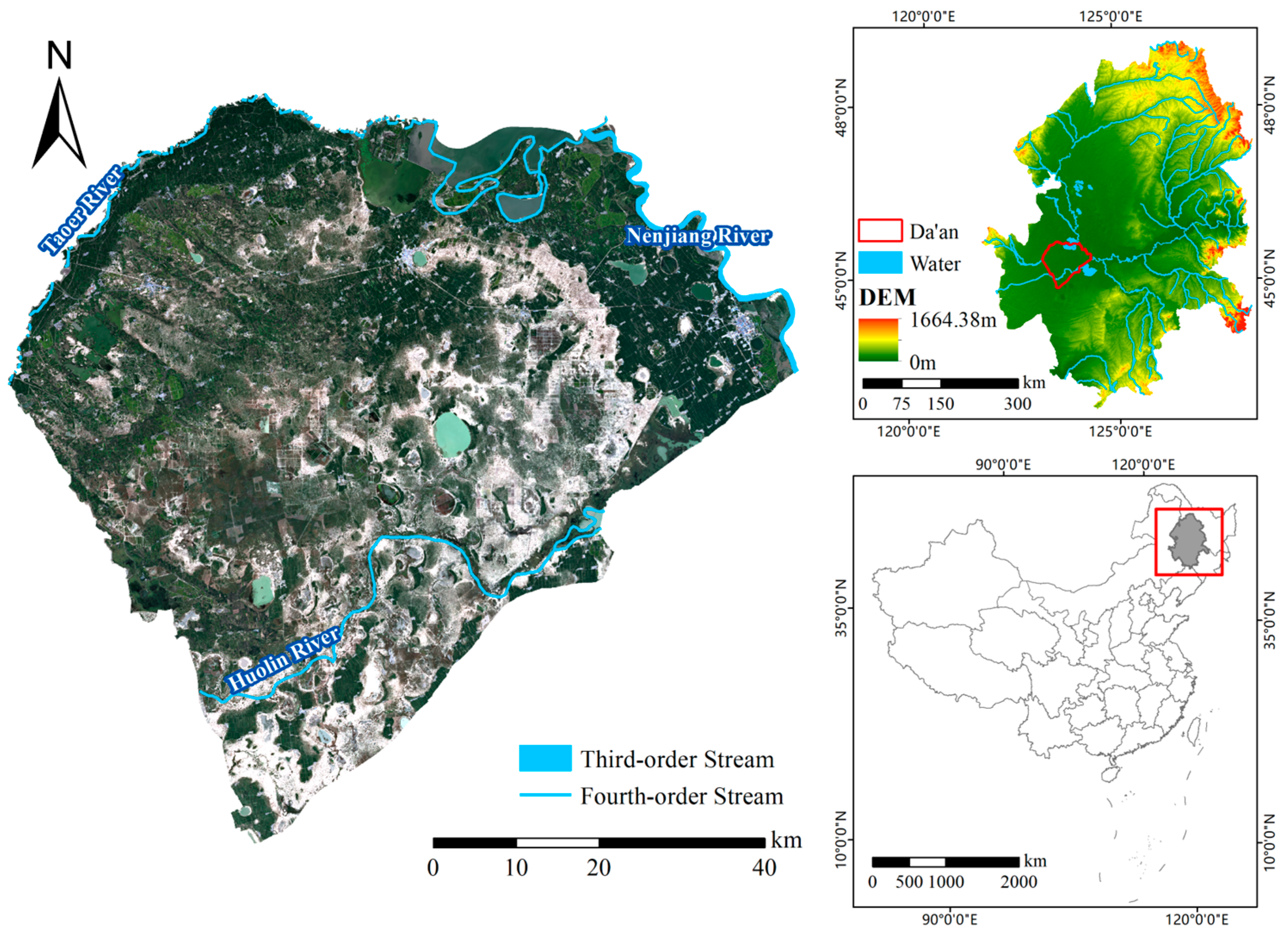
2.1. Study Area

Da’an City is located in the northwest of Jilin Province, in the hinterland of the Songnen Plain, with a total area of about 4879 km2. The location of the study area is shown in Figure 1. The terrain in this region is low-lying and flat, with a temperate, semi-humid continental climate and four distinct seasons. Da’an City is dominated by agriculture. It has abundant water resources but they are unevenly distributed, and seasonal floods and droughts occur from time to time. Da’an City is located in one of the world’s three major soda-type saline–alkali land regions, with a large area of concentrated contiguous saline–alkali lands. According to the data from the third Chinese national land survey, the area of saline–alkali land in Da’an City is about 640 km2, accounting for 13.1% of the total land area.

2.2. Data Sources and Preprocessing

In this paper, land use data from the 2000, 2010, and 2020 Chinese national land surveys, the data from permanent prime farmland (Figure 2), the data from ecological protection redlines (Figure 2), and data from the statistical yearbooks from 2001 to 2020 were used. These data were all from the Da’an City Bureau of Natural Resources. The 30 m land cover data from 2000 was from the National Geomatics Center (http://www.ngcc.cn/#/ accessed on 6 September 2023). The DEM data were from geospatial data cloud (http://www.gscloud.cn/#/ accessed on 13 January 2022) with a resolution of 30 m. The data on soil organic matter content was from the National Tibetan Plateau Data Center (http://data.tpdc.ac.cn/#/ accessed on 10 May 2023) with a resolution of 1 km.
The land survey data were reclassified into eight land use types such as cultivated land, forest land, grass land, construction land, wetland, water body, saline–alkali land, and other unutilized land (Table 1). The vector data were then converted into 30 m × 30 m raster data. In the first land survey, data were incomplete for the Da’an District, and the incomplete part was supplemented using 30 m resolution global land cover product data from 2000. The land use distribution is shown in Figure 3.
Through systematic analysis of land use simulation studies [33,34] and integrated consideration of the factors affecting the comprehensive improvement of saline–alkali land along with data availability within the target region, seven driving factors were selected, including DEM, slope, soil organic matter content (SOMC), soil salt content (SSC), distance to roads, distance to water bodies and distance to ditches. Although temperature and precipitation exert influences on the improvement of saline–alkali land, the spatial differences in temperature and precipitation in the small study area are not significant, and the impact on the growth probability of each land use type is not significant. Therefore, they were not considered. Furthermore, fertilizer application amount and diesel application amount were identified as critical contributors to the improvement saline–alkali land. These two factors were included in the nine driving factors selected for this study, as shown in Figure 4. Data on fertilizer application and diesel fuel use in towns and townships in Da’an City from 2001 to 2020 were extracted from the statistical yearbook and converted into 30 m raster data based on the spatial distribution of administrative areas. The data on SOMC were resampled to a resolution of 30 m to match the resolution of other spatial data.

2.3. Methods

The methodological framework of multi-scenario land use optimization simulation and comprehensive evaluation is shown in Figure 5. (1) In view of the characteristics of saline–alkali land accumulation in the study area, the spatial characteristics of land use types and driving factors of change were extracted using CNN and LSTM. The focus was on analyzing the potential for saline–alkali land and other unutilized land to be converted to cultivated land or ecological land. (2) The CNN-LSTM model was coupled with the PLUS model to simulate the spatio-temporal characteristics of land use change. Combining the CNN-LSTM model with the PLUS model’s spatial simulation capabilities, high-precision simulation of land use change in the study area was achieved, especially the refined prediction of saline–alkali land and other unutilized land to be developed and utilized. (3) Based on the Markov chain and MOP model, various scenarios for the development and utilization of saline–alkali land were constructed, including the historical development (HD) scenario, ecological protection (EP) scenario, land consolidation (LC) scenario, and sustainable development (SD) scenario. The constraints and optimization of the development and utilization of saline–alkali land were simulated under different scenarios with the CNN-LSTM coupled with the PLUS model, and the changes in the spatial pattern of land use and its impact on ESV, APB, and CB were systematically analyzed.

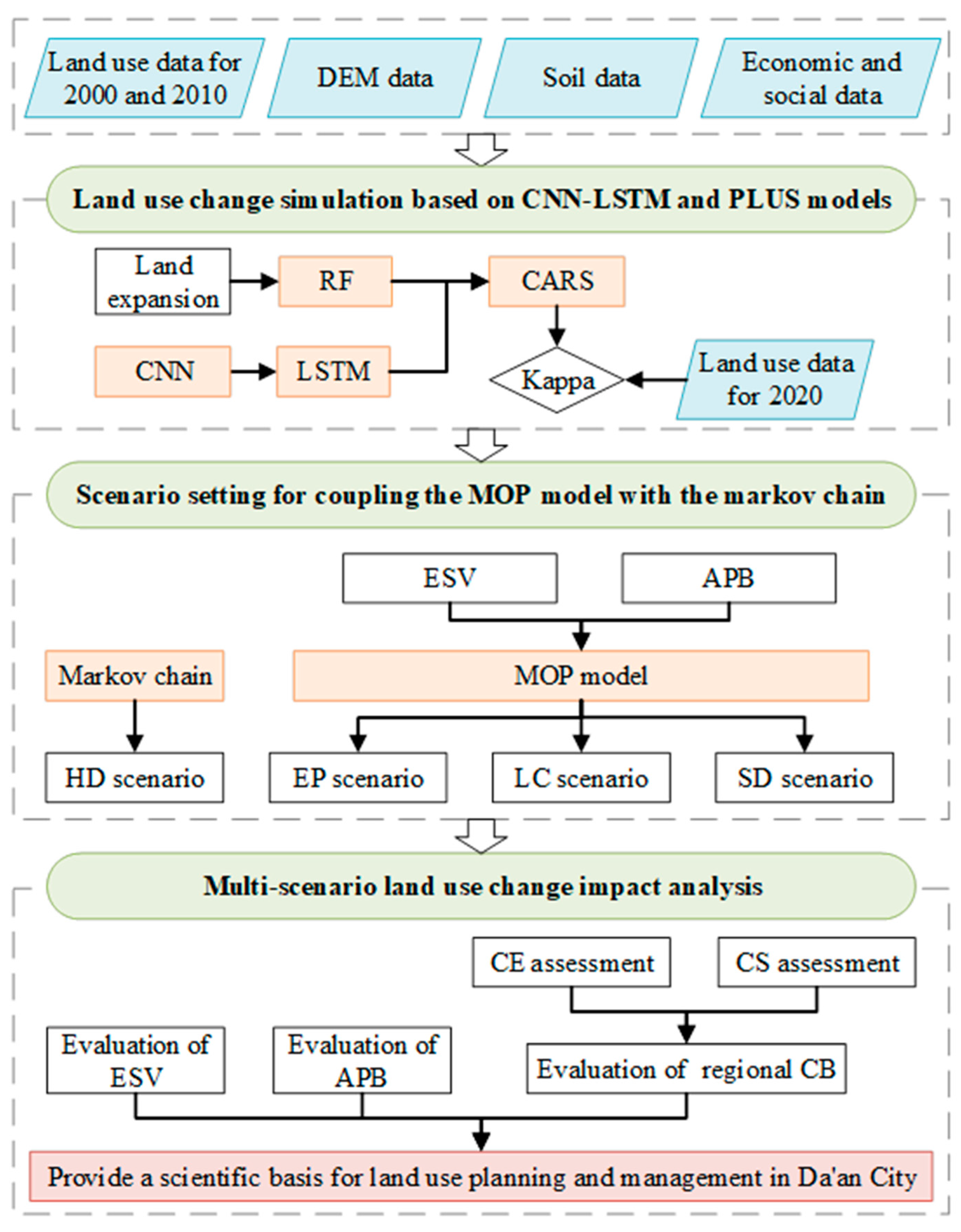
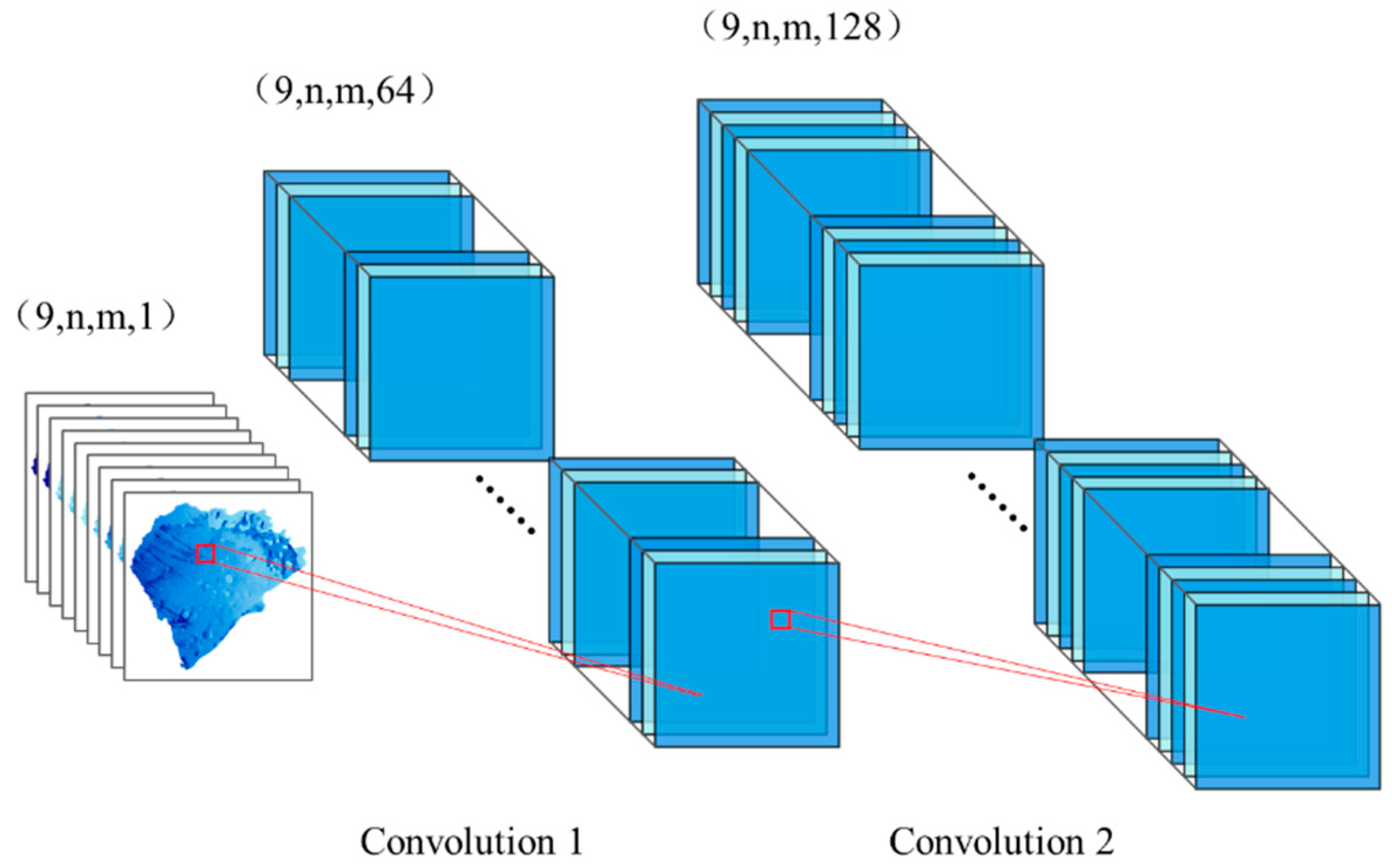
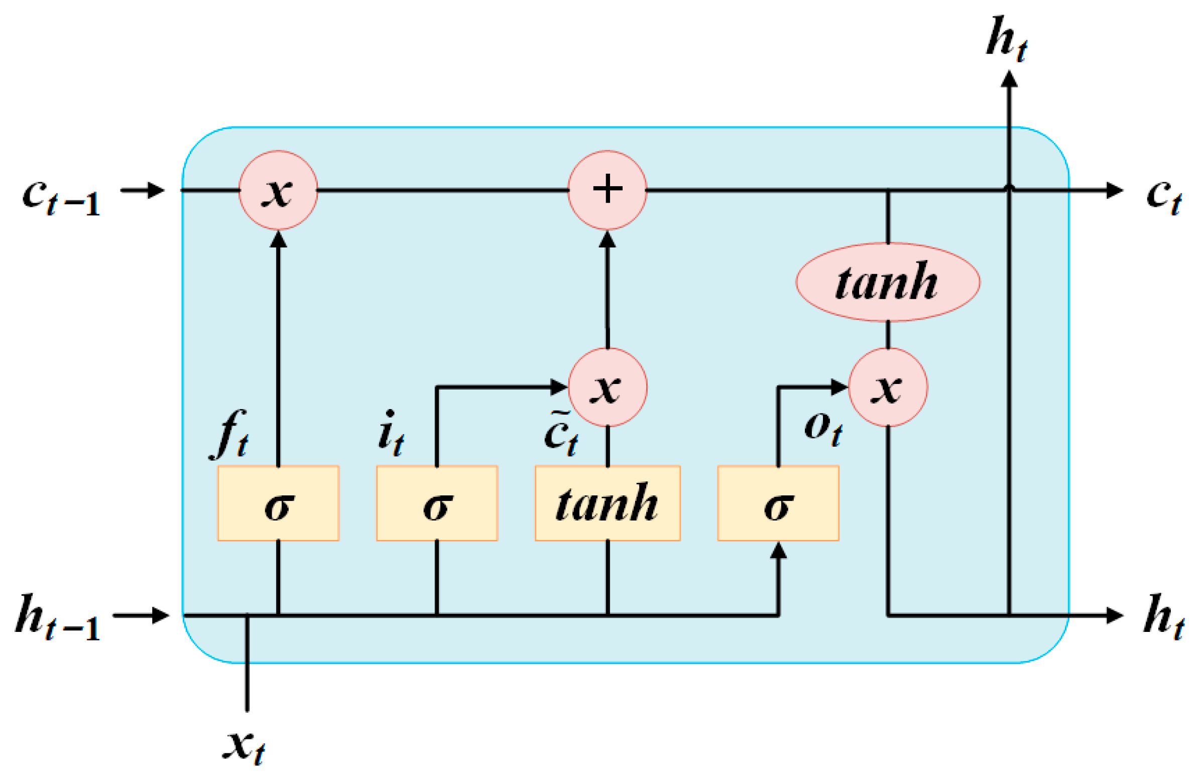
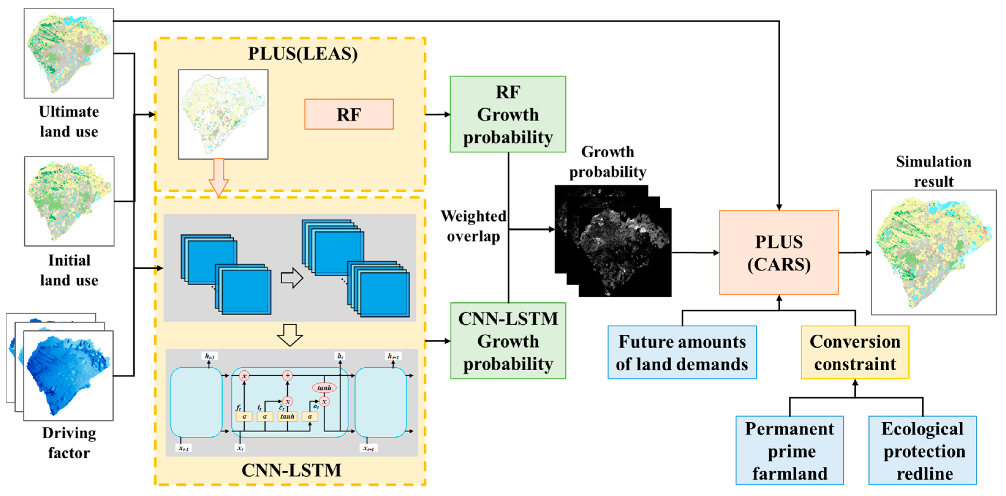
2.3.1. Land Use Change Simulation Based on CNN-LSTM and PLUS Models

PLUS is a land use change simulation model that integrates two modules: the land expansion analysis strategy (LEAS) and the CA based on multitype random seeds (CARS). In the LEAS module, land use change data of the two periods were analyzed to extract areas of land use expansion for each type of land use. Random forest (RF) is used to analyze the expansion areas and their driving factors in order to obtain the growth probability of each land use type. In the CARS module, a combination of random seed generation and a threshold reduction mechanism was used to dynamically simulate the autonomous generation of patches. And the changes in multiple land use types were simulated with the constraints on growth probability, neighborhood effects, adaptive coefficients, and transfer matrices.
For the RF model, the integration of decision trees with the sequential data was mainly relied on, so the ability to capture long-term dependencies in the data was weak. CNN-LSTM is different from the RF model; it combines the advantages of CNN in spatial information extraction with the ability of LSTM to capture long-term dependencies. PLUS has been improved by introducing a CNN-LSTM to replace the RF model in the LEAS module. In this paper, the CNN-LSTM was designed for a CNN with two convolutional layers and a model with a two-layer LSTM structure. In this model, the convolutional layer of the CNN was used to extract features. The basic operation is shown in Equation (1), and the schematic diagram is shown in Figure 6.
S c , d l = σ m i = 0 a j = 0 b b i , j l , m x c + i , d + j l 1 , m + e l
where l is the current layer; S c , d l is the output of the position (c,d); σ is the activation function; m is the number of features in the l 1 layer; b i , j l , m is the value of the convolutional kernel i , j ; a and b are the height and width of the convolutional kernel; e l is the bias term.
In LSTM, long-term memory is effectively maintained, and then long-term dependencies can be learned, which have advantages when processing long sequence data. The structure of LSTM is shown in Figure 7, and the calculation formula is as follows:
f t = s i g m o i d W f · h t 1 , x t + b f
i t = s i g m o i d W i · h t 1 , x t + b i
c ~ t = t a n h W c · h t 1 , x t + b c
c t = f t × c t 1 + i t × c ~ t
o t = s i g m o i d W o · h t 1 , x t + b o
h t = o t × t a n h c t
f t , i t and o t are the forget gate, input gate, and output gate; t is the current time step; t − 1 is the previous time step; W is the weight; b is the bias term; h is the hidden state; c is the cell state; c ~ is the candidate value of the unit state.
In this paper, the classic CNN-LSTM model structure was used [35]. In the input layer of the model 9, land use change driving factors, that is, 9 feature images with size n × m, were accepted. In the convolutional layer, the numbers of convolutional kernels in the two convolutional layers were 64 and 128, respectively; the convolutional kernel size was 3 × 3, and the sliding step was 1. During convolution, a circle of zeros was filled in around the edges of the feature image to ensure that the size of the input feature image remains the same and to avoid loss of information. After extracting spatial features by two convolutions, 9 feature maps of 128 × n × m were output. Next, these feature maps were divided into individual objects according to a grid, and the nine feature maps were combined into n × m objects containing 9 dimensions and 128 features. The land expansion data extracted by LEAS in PLUS was used as the label and input to the LSTM. The recurrent kernels of the two-layer LSTM structure were 64 and 96, respectively, and the time step was set to 9. Finally, through the fully connected layer, the growth probability of each land use type was output, including cultivated land, forest land, grass land, construction land, wetlands, water bodies, saline–alkali land, and other, unutilized land.
The output of the CNN-LSTM was weighted and fused with the growth probability calculated by the RF algorithm in PLUS to improve the accuracy of the land use conversion probability map. The fused probability map was input into the CARS module of PLUS, and the transfer matrix and neighborhood weight constraints that matched the actual situation in the study area were set. The permanent prime farmland and ecological protection redlines were used as areas constrained. Then, a simulation of the spatial distribution of land use change was finally completed. The structure of the coupled model is shown in Figure 8.
In this study, model validation was conducted using the Kappa coefficient to assess the agreement between the simulation results and the actual land use distribution. The Kappa coefficient is a statistical measure used to evaluate the consistency between classified results and actual observations, effectively accounting for the influence of random agreement. Specifically, a confusion matrix was constructed by comparing the simulation results with the actual land use distribution, and the Kappa coefficient was calculated to evaluate the consistency between the two. The formula for calculating the Kappa coefficient is as follows:
K a p p a = P o P e 1 P e
where P o is the overall accuracy, which is the proportion of areas where the simulation results are consistent with the actual land use distribution; P e is the accidental consistency between the simulation results and actual land use distribution. The Kappa coefficient ranges from −1 to 1. Kappa close to 1 indicates that the simulation results are more similar to the actual distribution.

2.3.2. Scenario Setting for Coupling the MOP Model with the Markov Chain

(1)
ESV and APB
The impact of land use change on ESV and APB is directly related to the scenario setting for the development and utilization of the regional saline–alkali land. In order to quantitatively evaluate the ESV and APB, the ESV coefficient and APB coefficient of each land use type (Table 2) were determined based on regional characteristics and the relevant literature [36]. Then, the ESV and APB of the area were assessed by the area of each land use type. The calculation formula are as follows:
E S V = i = 1 8 E i x i
APB = i = 1 8 A i x i
E i is the unit area ESV of land type i; A i is the APB benefit coefficient of land type i; and x i is the quantity of land type i, which can be cultivated land, forest land, grass land, construction land, wetland, water body, saline–alkali land and other unutilized land, respectively.
(2)
Scenario setting for the development and utilization of saline–alkali land in the region
In order to explore the changes in saline-alkali land development and utilization under different policies and management paths, a policy-guided land use optimization simulation experiment was constructed with the development needs of the study area. Four regional saline–alkali land development and utilization scenarios of historical development (HD), ecological protection (EP), land consolidation (LC), and sustainable development (SD) were set up as follows: (1) In the HD scenario, the path that land use change simulated in the study area is likely to follow in the absence of new policy interventions or technological innovations. (2) In the EP scenario, ecological benefits were maximized by optimizing land use and implementing ecological restoration projects based on the ecological protection redline system and wetland protection policies. (3) In the LC scenario, the national land consolidation policies were combined with saline–alkali land treatment technologies to improve the soil quality and productivity of saline–alkali land through engineering management and agricultural technology so as to expand the area of cultivated land and improve agricultural efficiency. (4) In the SD scenario, the ecological and agricultural benefits were comprehensively considered, emphasizing the versatility of saline–alkali land development and utilization. Guided by Sustainable Development Goals (SDGs), the land use pattern was optimized through systematic governance and reasonable layout, achieving synergy between ecological protection and economic development.
In this paper, Markov chains were used to model the transition process of land use change. For the HD scenario, a transition matrix was constructed based on land use change data from 2010 to 2020, and the land use pattern in 2030 was predicted. For the EP, LC, and SD scenarios, the land use pattern in the HD scenario for 2030 was further optimized with the MOP model to maximize ecological and agricultural benefits under different scenarios. The MOP model is a mathematical model that finds an optimal solution between multiple objectives. The model includes decision variables, objective functions, and constraints, which are expressed by the following formula:
f 1 x = m a x i = 1 n E i x i
f 2 x = m a x i = 1 n A i x i
f 3 x = m a x f 1 x , f 2 x
s . t . = i = 1 n c i j x i = , d i ,     j = 1,2 , , m x i 0 ,     i = 1,2 , , n
where f 1 x , f 2 x , f 3 x are the objective functions for the EP, LC, SD scenarios; n is the number of decision variables; x i represents decision variable i ; E i , A i are ESV coefficients and APB coefficients of land type i ; c i j is the coefficient of decision variable i in constraint j ; m is the number of constraints; d i is the constraint value. The model constraints are shown in Table 3.

2.3.3. Multi-Scenario Land Use Change Carbon Balance Analysis

In order to assess the impact of saline–alkali land development and ecological protection policies on the regional balance of carbon source and carbon sink, the regional carbon balance under different scenarios was quantitatively estimated by calculating the changes in carbon emissions (CEs) and carbon storage (CS). CEs were calculated based on the amount of land use types and their corresponding CE coefficients. The CE coefficient reflects the amount of CEs per unit area that were produced annually by the human being activities such as farming, fertilizing, and deforestation for a particular type of land use. According to the relevant literature [38,39], the CE coefficients for different land use types are shown in Table 4, and the formula for calculating total CE is as follows:
C E = i = 1 8 C E C i x i
C E C i is the carbon emission coefficient of land use type i ; x i is the area of land use type i .
The estimation of CS is based on the CS density calculating method, which is affected by both soil CS and plant CS. In this paper, the relevant literature [38,40] were referenced to determine the CS density parameters for different land use types, as shown in Table 4. Total CS are calculated using the following formula:
C S = i = 1 8 C S D i x i
C S D i is the carbon storage density of land use type i ; x i is the area of land use type i .
CB refers to the difference between carbon sink and CEs in a certain area [41], reflecting the combined effect of land use changes on regional carbon cycles under different scenarios. By comparing the CB under different scenarios, the effect of land use change on enhancing or weakening the carbon sink capacity was analyzed, the CE and CS dynamics of different land use types were revealed, and the contribution of regional land resource optimization strategies to mitigating CE and enhancing carbon sink capacity were clarified. The formula for calculating CB is as follows:
C B = C S f i n a l C S i n i t i a l C E f i n a l
C S f i n a l and C S i n i t i a l are the CS in 2030 and 2020; C E f i n a l is the CE in 2030.

3. Results

3.1. Multi-Scenario Land Use Simulation Analysis in 2030

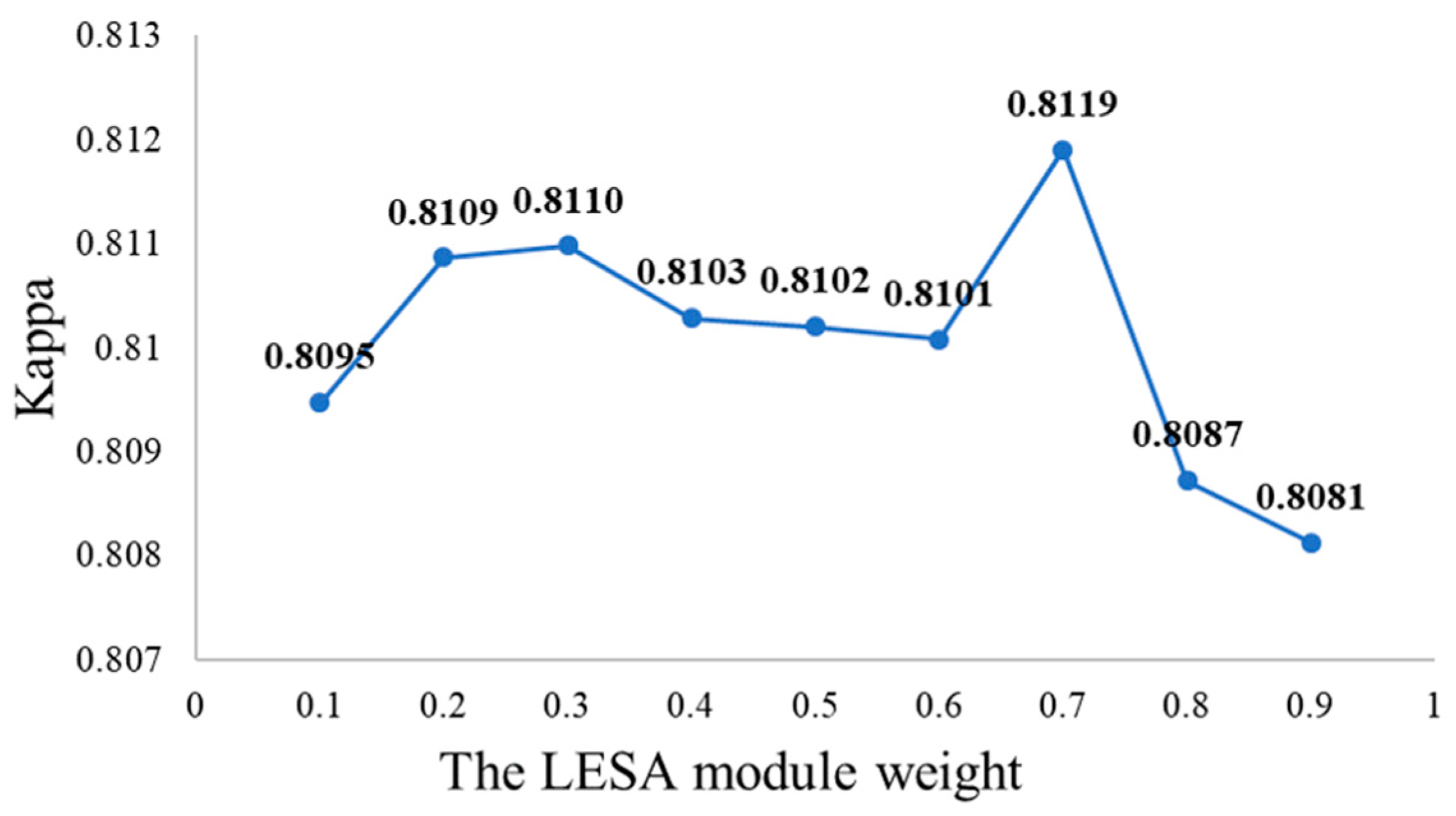
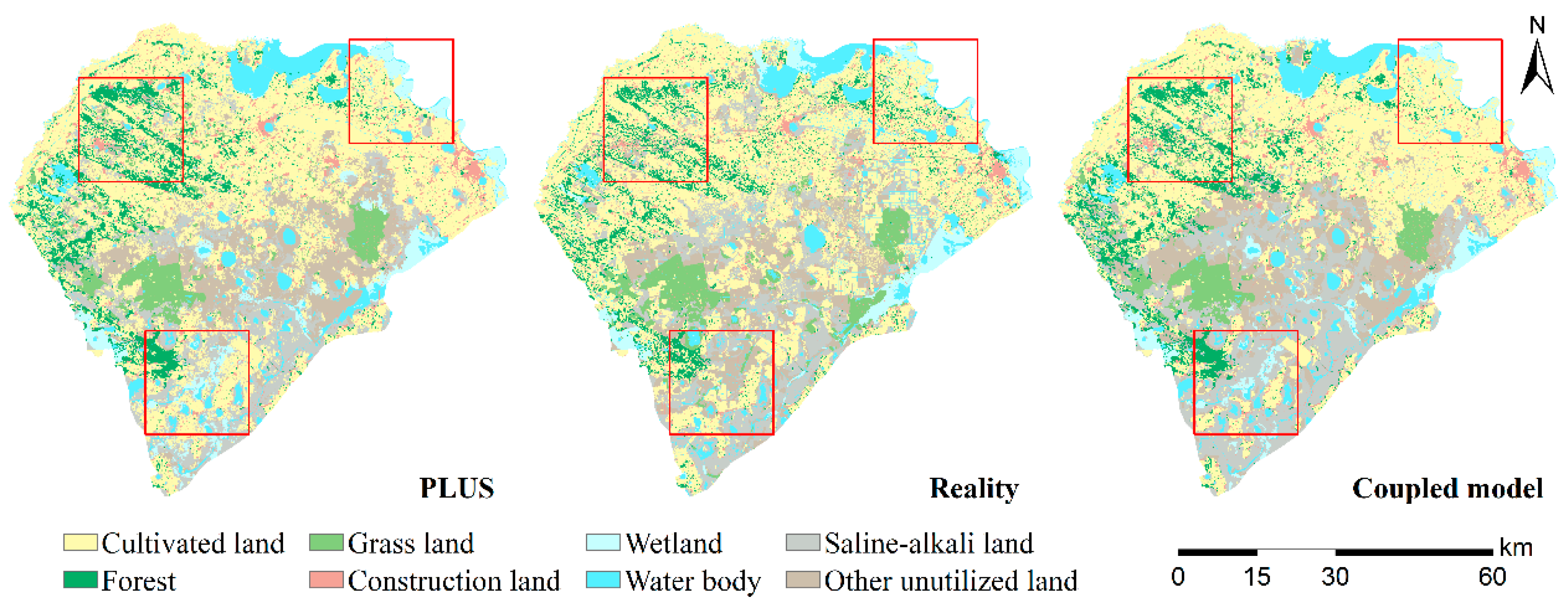
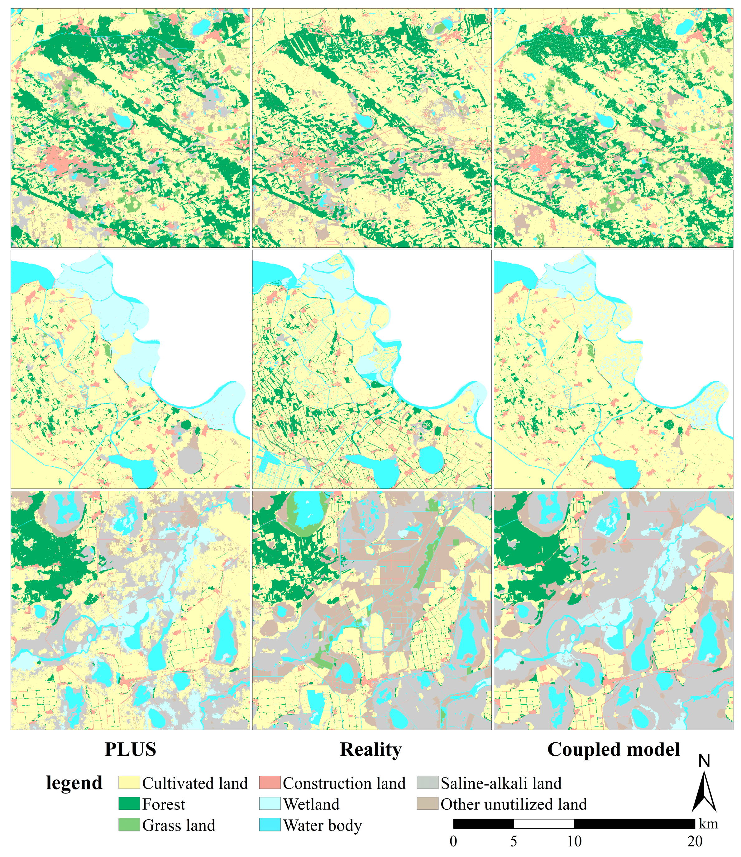
3.1.1. Accuracy Analysis of CNN-LSTM and PLUS Coupled Models

In order to improve the accuracy of the calculation of the growth probability in land use change simulation, the coupled method based on the LEAS module in PLUS and CNN-LSTM proposed in this paper was used. By analyzing land use data from 2000 to 2010 in Da’an City, Jilin Province, the growth probability of each land use type was calculated using the LEAS model and CNN-LSTM, respectively, and the two were weighted and fused. The growth probability after the merger was used to simulate the land use pattern in 2020. The simulation results were verified by comparing them with the actual land use distribution data in 2020. The Kappa was obtained as shown in Figure 9. The horizontal axis of the figure was the LESA module weight, and the vertical axis was the Kappa of the simulation result. The higher the Kappa, the better the simulation effect. When the weight of the LESA module was set as 0.7, the weight of the CNN-LSTM was set as 0.3. Then, the simulation results were optimal. With the weights, the Kappa was 0.8119, which was better than the consistency standard of 0.75 [42,43]. This shows that the improved model has a significant advantage in simulation accuracy.
The growth probabilities of each land use type under the optimal weight were entered into the CARS module of PLUS to simulate the land use pattern of Da’an City in 2020. A comparison of the simulation results of different models with the actual distribution was shown in Figure 10. The left figure is the simulation results of PLUS, the middle figure is the actual distribution, and the right figure is the results of the coupled model. The three areas marked on the figure are the main areas where the differences between the two simulation results and the actual distribution occur. From left to right and from top to bottom, they are the areas where cultivated land and ecological land are intermingled, the areas where rivers and wetlands are distributed, and the areas where cultivated land and saline–alkali land are intermingled. A local comparison of the three areas is illustrated by Figure 11. In areas where cultivated land and ecological land were intermingled, a more obvious continuous block distribution was shown by the forest in the PLUS results, which was inconsistent with the actual scattered distribution. The coupled model simulation results were closer to the actual distribution. In the area of rivers and wetlands, the coupled model simulation results were closer to the actual striped distribution, while a patchy distribution of wetlands was shown by the PLUS results. In the area where cultivated land and saline–alkali land were intermingled, the characteristics of the concentrated and contiguous distribution of saline–alkali land and other unutilized land were reproduced by the coupled model, while the saline–alkali land and other unutilized land were too easily converted into cultivated land, with a more scattered distribution, failing to show the actual spatial agglomeration characteristics.

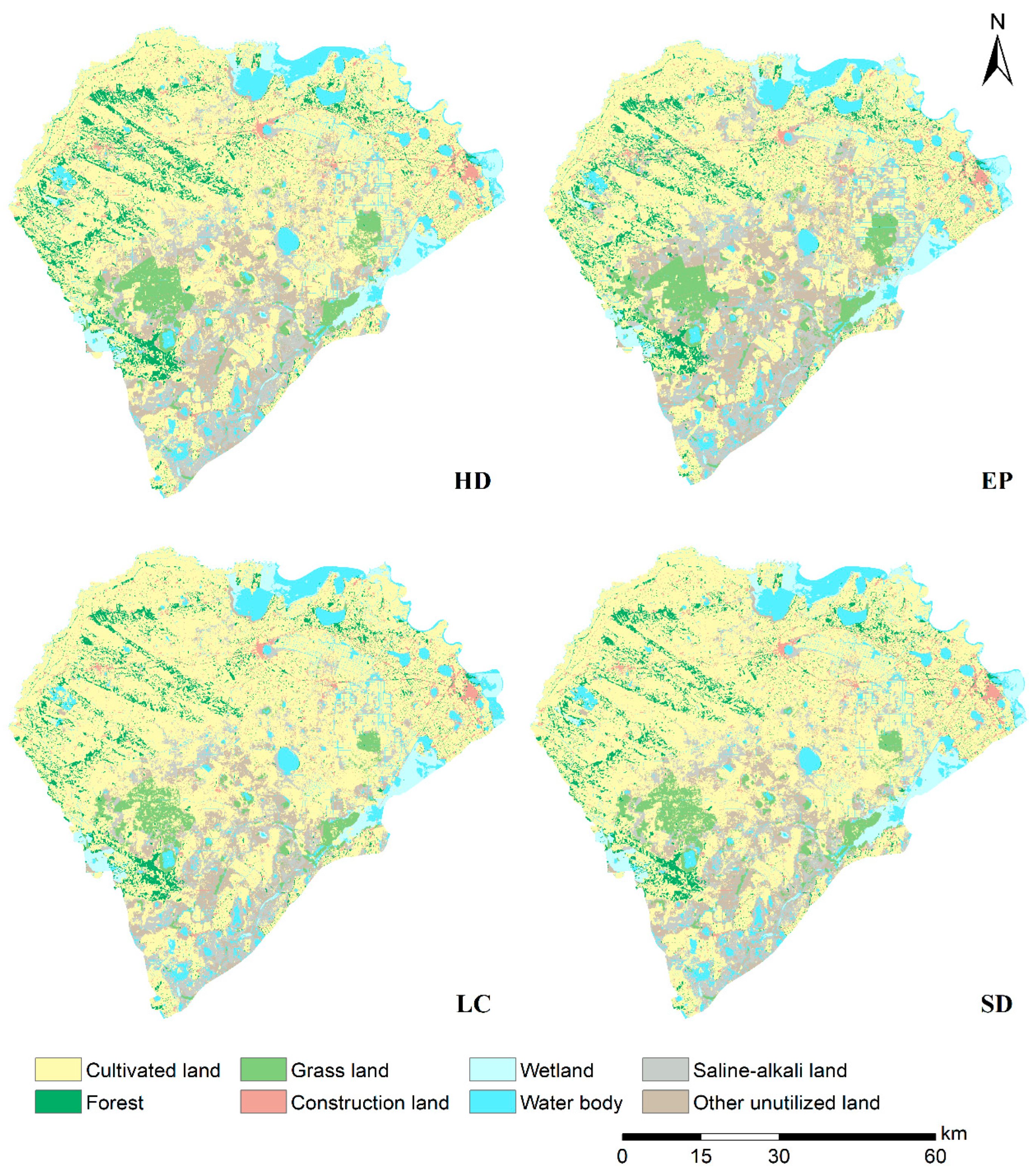
3.1.2. Multi-Scenario Land Use Simulation Results and Analysis for 2030

In order to evaluate the trend of land use change under different policy orientations, in this paper, a transition matrix was constructed based on land use data in 2010 and 2020, and a Markov chain was used to simulate the amount of each type of land use in 2030 under the HD scenario. For the EP, LC, and SD scenarios, the MOP model was used to set up a multi-objective function and constraints to calculate the quantity of each land use type under different scenarios. Finally, the land use quantities for each scenario were input into the CNN-LSTM and PLUS coupled model. At the same time, the ecological protection redlines and the scope of permanent prime farmland were used as conversion constraints to simulate the land use pattern of Da’an City in 2030. The amount and proportion of land use in each scenario are shown in Table 5 and Figure 12.
There are significant differences in the quantitative ratio and spatial distribution of land use in different scenarios, as shown in Figure 13. In the LC scenario of 2030, priority was given cultivated land expansion, which accounts for the largest proportion this scenario, at 62.50%. Due to policies favoring the development and utilization of saline–alkali land and other unutilized land, the amount of these land use types in 2030 has decreased significantly, by 33.02%, compared to 2020. At the same time, the proportion of ecological land in this scenario was relatively small, at only 27.97%. The spatial distribution of ecological land was relatively limited, failing to form a large-scale ecological network. In the EP scenario of 2030, the area of cultivated land increases slowly, the area of ecological land remained at a relatively high level, and saline–alkali land and other unutilized land were widely distributed, forming a relatively continuous ecological corridor. In this scenario, cultivated land accounts for the smallest proportion, while ecological land accounts for the largest proportion, at 51.23% and 35.96%, respectively. Under this scenario, more land use patches were converted to ecological land, which reflects the priority of ecological protection. In the SD scenario for 2030, the cultivated land and ecological land account for a relatively balanced proportion of 61.47% and 29.00%, respectively. More saline–alkali land and other, unutilized land were converted into cultivated land or ecological land, mainly in the southern region, which shows the optimization and efficient allocation of land use. In the HD scenario for 2030, the number of each land use type shows a historical development trend, with no significant tendency, similarly to the distribution of land use types in 2020.

3.2. Land Use Change and Impact Assessment in Different Scenarios

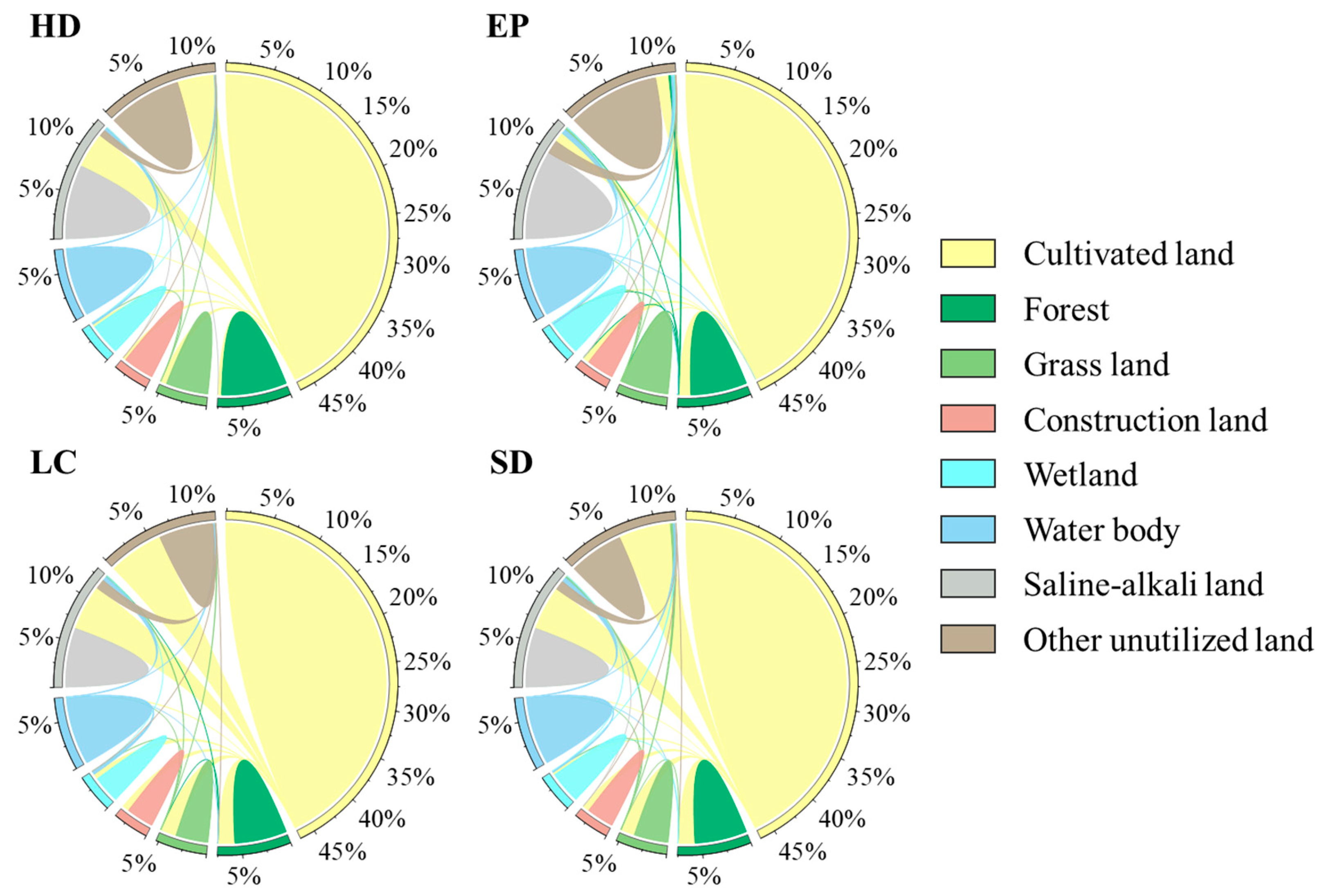
3.2.1. Analysis of Land Use Change from 2020 to 2030

Based on the superimposed analysis of the land use patterns in 2030 under four scenarios in Da’an City and the land use distribution in 2020, the trend of land use change in Da’an City from 2020 to 2030 was shown in Figure 14. The growth probability is shown in Table 6, where ecological land includes forest, grass land, wetland, and water body. In the simulated HD scenario for 2030, the current pattern was continued, with cultivated land remaining relatively stable, while the development and utilization of saline–alkali land and other unutilized land was more significant, with the conversion rates of 38.28% and 34.67%, respectively. In the simulated EP scenario for 2030, the protection of natural resources and ecosystems was emphasized. Ecological protection areas were relatively stable in this scenario. Saline–alkali land and other unutilized land were less developed, and only 8.26% and 11.92% have been converted to cultivated land. In the simulated LC scenario for 2030, a strong prioritization of the development of agricultural production was shown. Cultivated land has expanded significantly, with the area of newly cultivated land reaching 34.20%. Saline–alkali land and other unutilized land were converted to cultivated land in large quantities, with the conversion rates of 49.09% and 37.78%, respectively. There has been a significant reduction the area of forest, grass land and wetlands, with the conversion rates of 24.56%, 33.41% and 24.82%, respectively. In the simulated SD scenario for 2030, a balance between ecological protection and land use and development in land use change was formed. Saline–alkali land and other unutilized land were converted into cultivated land in large quantities, with the conversion rates of 46.43% and 36.85%, respectively. Ecological land was also highly stable, with forest, grass land, wetland and water body retention rates as high as 75.44%, 70.43%, 88.68% and 99.28%. In the simulated land use changes in the four scenarios for 2030, the significant influence of policy goals was reflected. The HD scenario was biased towards maintaining the status quo, with limited improvement in ecological functions. In the EP scenario, the overall improvement of the ecosystem was highlighted, and the protection and expansion of ecological protection land was most significant. In the LC scenario, efficient development of land resources was focused on, highlighting the expansion of cultivated land, but the pressure was put on the ecosystem. In the SD scenario, a good balance between ecological protection and agricultural production was stricken, achieving a win–win situation through the reasonable development of saline–alkali land and other unutilized land.

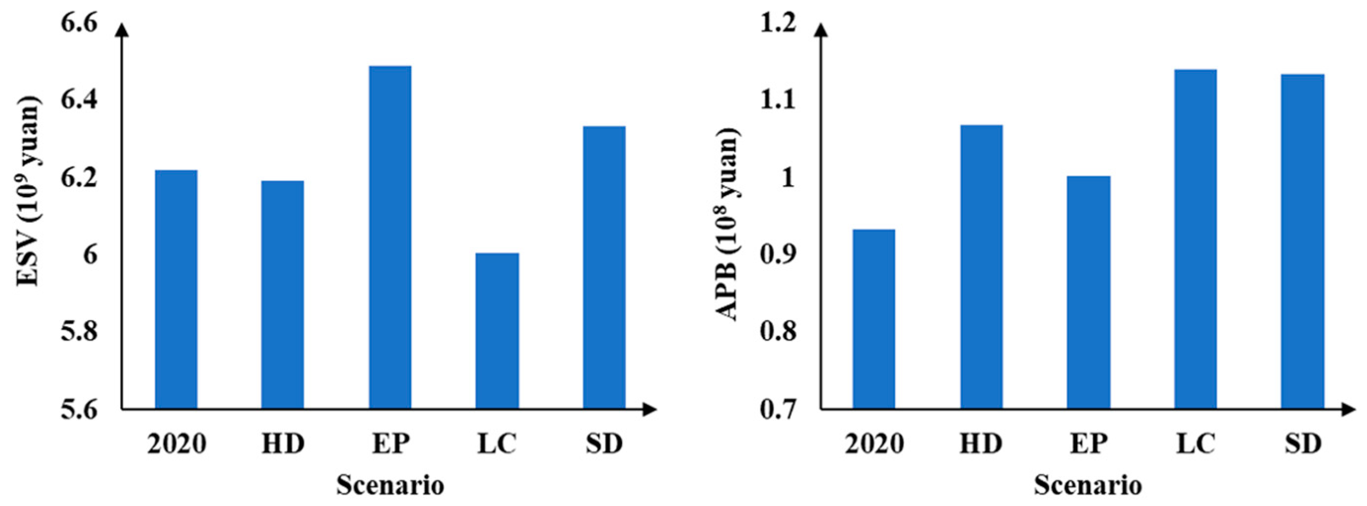
3.2.2. Assessment of Land Use Change Effects

In different scenarios, significant differences were found in both the ESV and APB of the study area, as shown in Figure 15. To the simulated EP scenario for 2030, the maximization of ESV was emphasized. In this scenario, ESV was the highest and APB was the lowest. ESV was increased by 4.36% compared to 2020, while APB only was increased by 7.33%. The service capacity of regional ecosystems was enhanced with the policies of ecological protection. In particular, the expansion of ecological land, such as forests and wetlands, plays a key role in significantly enhancing ecological benefits. In the simulated LC scenario for 2030, the improvement of APB was prioritized. In this scenario, ESV was the lowest and APB was the highest. ESV was 3.44% lower than in 2020, while APB was 22.11% higher than in 2020. Agricultural productivity has increased significantly due to the consolidation of saline–alkali land and the expansion of cultivated land, while the development of ecological land has been restricted due to the large-scale expansion of cultivated land. In the simulated HD scenario for 2030, there were no significant advantages in terms of ecological and agricultural efficiency. In this scenario, the ESV basically maintains the status quo, with a decrease of only 0.4%, while the APB has a limited increase of only 14.38% compared to 2020. In the absence of policy intervention, the potential for improving ecological and agricultural benefits through land use changes was limited. In the simulated SD scenario for 2030, a better balance between ecological and agricultural goals was achieved through coordination, with strong potential for sustainable development. Compared with 2020, ESV was increased by 1.83% and APB increased by 21.41%. in this scenario, a good balance between ecological protection and development and utilization was struck.

3.3. The Impact of Land Use on CB in Different Scenarios

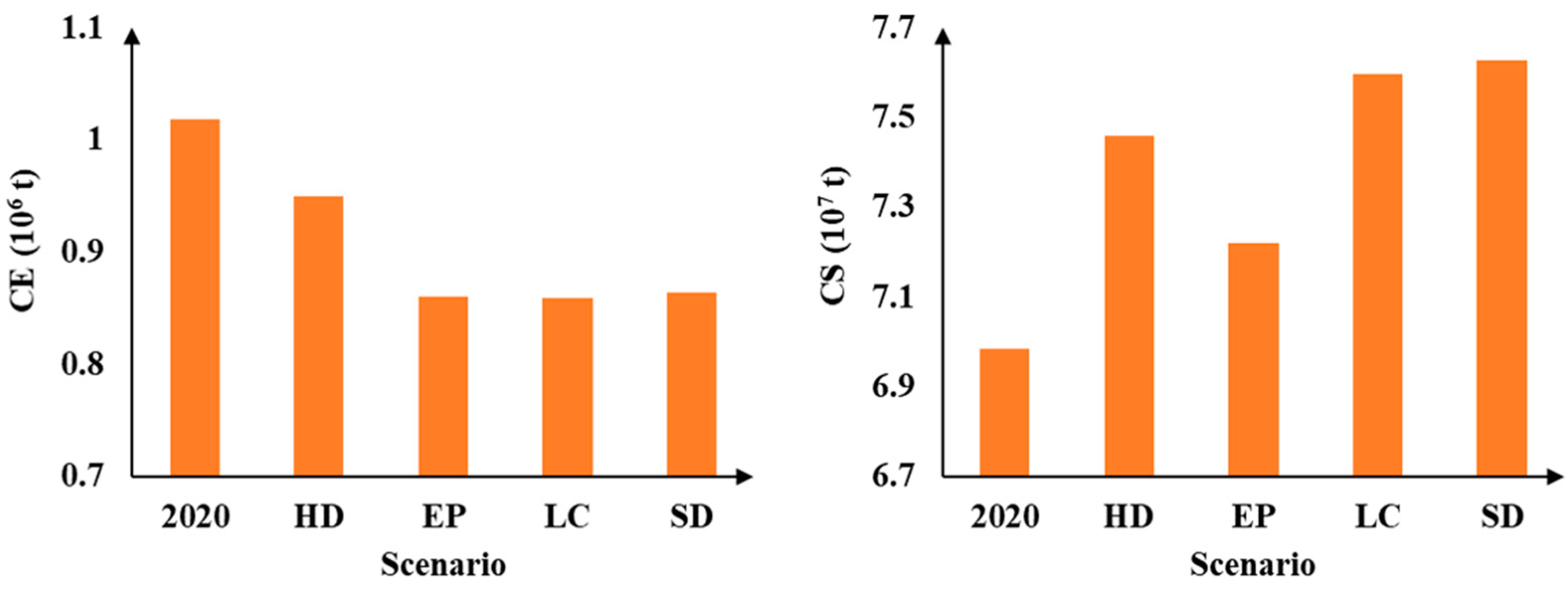
3.3.1. Analysis of CE and CS in Different Scenarios

CE and CS in the study area in 2030 were calculated based on the results of land use simulation in four scenarios, combined with the CE coefficient and CS density of each land use type, as shown in Figure 16. The CE of the four simulated scenarios for 2030 was significantly lower than that of 2020. Among them, the HD scenario had the highest CE of 949,600 tons, a 6.17% decrease compared to 2020. The reduction in CE was limited without policy intervention. The CEs of the EP, LC, and SD scenarios were similar, at 859,700 tons, 859,300 tons, and 864,000 tons, respectively, representing reductions of 15.54%, 15.58%, and 15.12% compared to 2020. Whether saline–alkali land was developed and utilized or ecological protection was carried out, which has a significant effect on reducing CE, because the CEs in all three scenarios were significantly lower than in the HD scenario. Although the CEs of the three scenarios were close, there was still a slight difference. LC scenarios had the lowest CEs, which shows that saline–alkali land development and utilization play a more critical role in reducing the region’s CEs.
The trend of change in CS in each scenario shows significant differences to the changes in land use structure. The CS of the LC and SD scenarios in 2030 were 759.622 million tons and 762.649 million tons, respectively, which was significantly higher than that of the HD and EP scenarios. This was mainly due to the improvement in saline–alkali land and the enhancement of carbon sink capacity through land consolidation. Among these, the SD scenario was slightly higher than the LC scenario, in which the comprehensive protection of CS was reflected by the policy of balancing ecological protection and agricultural development. The CS of the HD scenario was 74.5914 million tons, an increase of 6.79% compared to 2020. The CS of the EP scenario was 72.2019 million tons, which was lower than in the other three scenarios, but still higher than that of 2020, with an increase of 3.37%. By increasing the area of land with a high CS capacity, such as ecological land, a positive impact on regional CS will be achieved, but the enhancement capacity will be limited, as it will be much smaller than the enhancement capacity of regional CS brought about by the development, treatment, and utilization of saline–alkali land. Overall, the HD scenario shows the smallest change, which indicates the need for policy intervention. A significant reduction was achieved in CE with the EP, LC, and SD scenarios, while a two-way improvement was achieved in CE control and CS with the SD scenario.

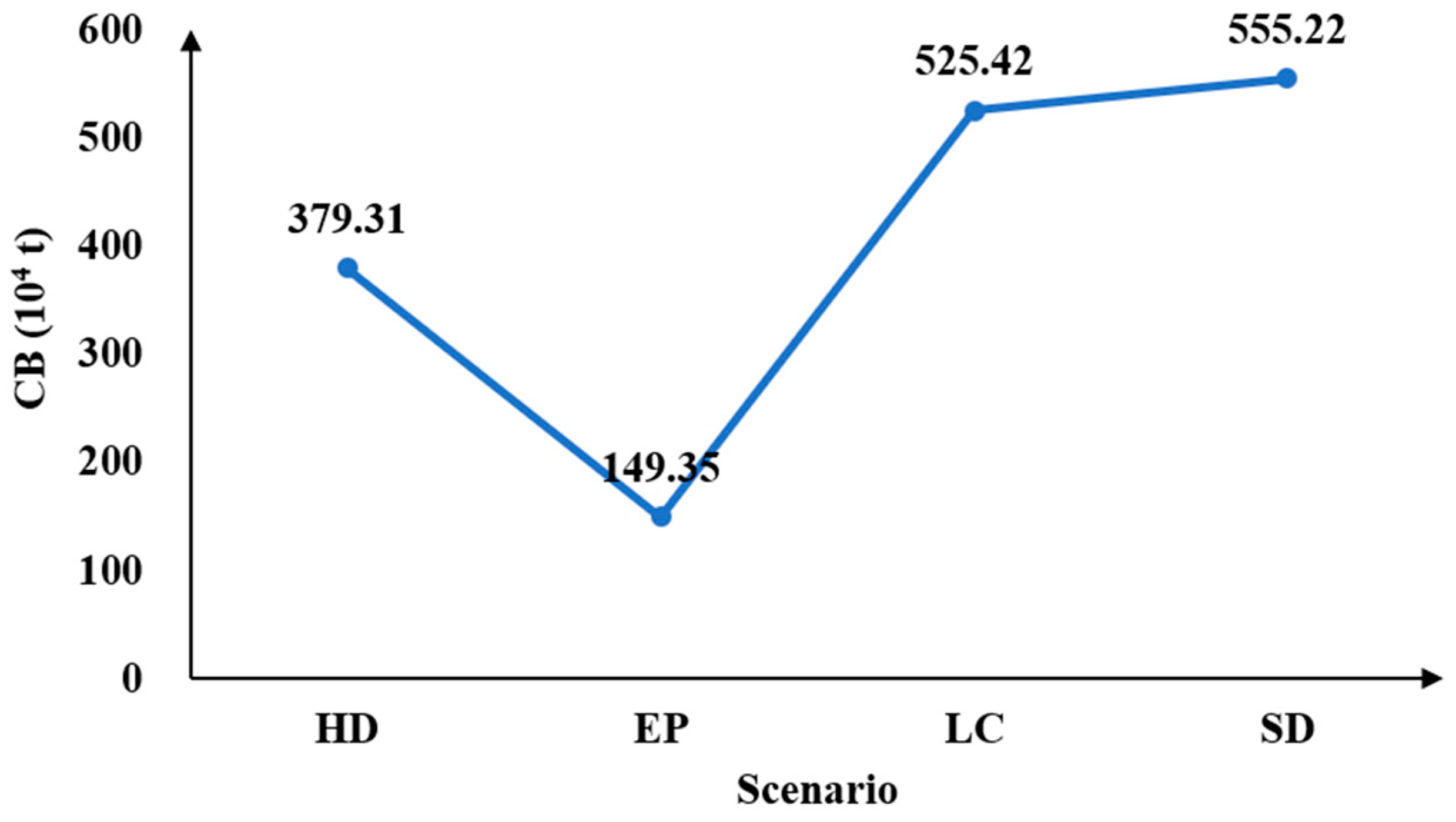
3.3.2. Regional CB Change Trends Under Different Policy Orientations

Based on the analysis of CEs and CS under different scenarios simulated in 2030, the regional CB in each scenario was calculated to measure the comprehensive carbon effect of different policy orientations, as shown in Figure 17. The SD scenario had the highest CB of 5,552,200 tons, and successfully achieved coordinated development of ecological protection and agricultural production. LC was second, at 5,254,200 tons. Although in this scenario, the cultivated land area significantly increased and the carbon sink capacity was enhanced through large-scale saline–alkali land consolidation, further improvement of CB was limited with the increasing CEs. The EP scenario had the lowest CB of 1,493,500 tons. Although with the ecological protection policies, the carbon sink capacity was enhanced by expanding ecological land, the growth of CS was constrained due to the low intensity of development of saline–alkali land and other unutilized land. The CB of the HD scenario was 3,793,100 tons, which was much lower than that in the LC and SD scenarios. In the natural development patterns, the effect of optimizing CB was limited. Overall, the CB of the simulated scenarios for 2030 under different policy directions showed significant differences. The SD scenario was optimal in terms of balancing agricultural production and ecological protection, which provides an effective path for sustainable development in the region. In the LC scenario, the CS significantly increased through land consolidation. But, CEs needed to be further controlled. The EP scenario was outstanding in terms of enhancing carbon sink capacity, but its contribution to the CB was relatively limited. Without policy intervention, it was difficult to significantly optimize the CB in the HD scenario.

4. Discussion

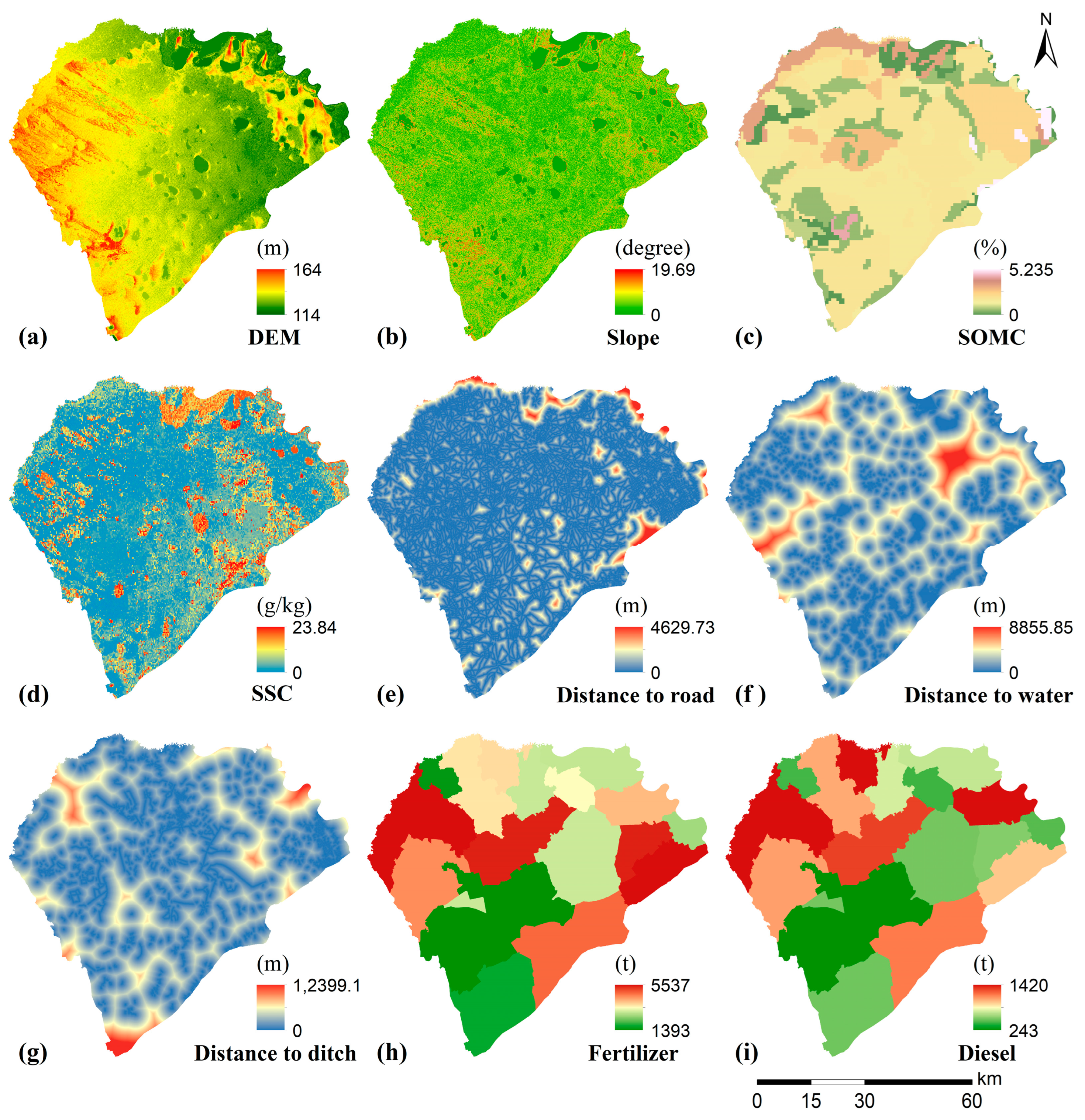
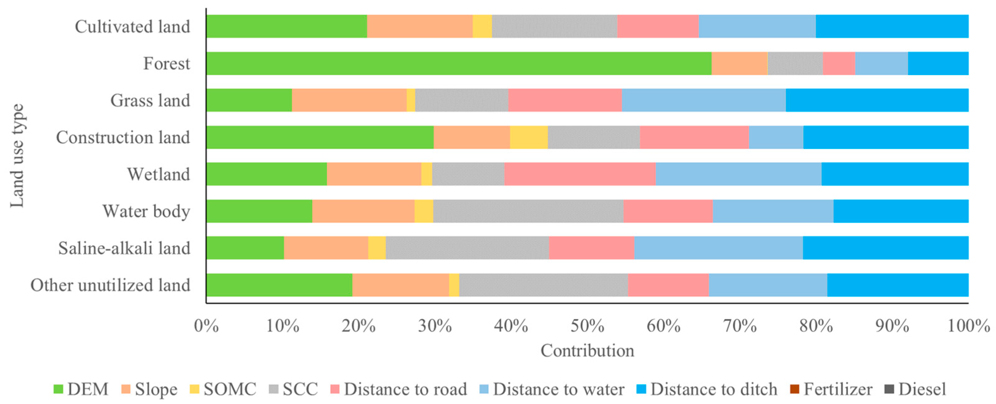
4.1. Analysis of the Contribution of Driving Factors

In the land use change simulation, the contribution of driving factors reveals the impact of different influencing factors on the conversion between land types. In this study, nine driving factors were selected, including DEM, slope, SOMC, SSC, distance to road, distance to water body, distance to wetland, fertilizer application amount, and diesel application amount. The contributions of different driving factors to the growth probability of each land use type varied significantly. As shown in Figure 18.
The driving factors exerting the most significant influence on land use change were DEM, distance to ditch, distance to water body, and SSC. This is because these factors play a crucial role in optimizing land use in cultivated land reserve resource areas rich in saline–alkali land. The most significant land use change in Da’an City was the conversion of saline–alkali land and other unutilized land into cultivated land. Topographical factors, water resources, and soil salinity restricted the development and utilization of land in this area. In contrast, SOMC, fertilizer application amount, and diesel application amount exhibited relatively weaker effects on land development and utilization in this area. especially the latter two, which exhibited a negligible impact on land use change in the study area. This reflected that natural factors were given more consideration in site selection for saline–alkali land improvement and utilization.
There were also significant differences in the sensitivity of different land use types to different driving factors. Cultivated land and forest were most sensitive to DEM, with driving factor contributions of 21.11% and 66.29%, respectively. This shows that the development of cultivated land and forest was restricted in areas with large terrain undulations. Grass land and wetland were the most sensitive to distance to water bodies, with driving factor contributions of 21.49% and 21.78%, respectively. This indicates that these land use changes were mainly affected by water resources, and areas closer to water bodies were more likely to become grass land and wetland. Water bodies, saline–alkali land, and other unutilized land were most sensitive to SSC, with contributions of 24.99%, 21.40%, and 22.15%, respectively. This indicates that SSC directly affected the ease with which an area developed into saline–alkali land and other unutilized land. In addition, areas with higher SSC were more likely to become lakes.

4.2. General Applicability and Limitations of Coupling CNN-LSTM with PLUS to Simulate Land Use Change

In this paper, the coupled CNN-LSTM and PLUS model shows significant advantages in capturing the complex dynamics and spatially driven mechanisms of land use change. The applicability of this model was not limited to this study area but was also applicable to similar cultivated land reserve resource areas, such as Xinjiang [44], Gansu [45], and Yunnan [46] in China, as well as to other agricultural areas, such as Greece [47], Thailand [48], and India [49,50]. For promotion and application in different environments and regions, different driving factors and scenario constraints can be selected based on the regional characteristics and policy requirements of the study area. However, there are limitations in the model. First, the model is highly dependent on the quality and resolution of the input data. Areas with missing or insufficient data may lead to a significant decrease in simulation results. Second, the application of the model to large areas or longer time scales is limited by the high computational complexity. In addition, if the driving factors selected do not fully reflect the actual situation, the simulation results may be biased. In the future, the optimized algorithms should be explored with low computational costs and further expand the model’s adaptability to multi-source heterogeneous data.

4.3. Evaluation of Land Use Effects Under Multi-Scenario Simulation

In this paper, four land resource optimization scenarios were set up to simulate the optimal path of land resources under different policy orientations in 2030. The simulation results of different scenarios were evaluated. The evaluation results shared similarities with similar studies in other regions but also reflected regional characteristics. Previous research predominantly evaluated ESV, economic effects, and CB, while studies assessing APB remain scarce. ESV is often the most focused effect in studies. Ecological protection-related scenarios [51,52] are included in the scenario settings of many studies. In these studies, the ESV of ecological protection-related scenarios was significantly improved. Some studies focused on cultivated land protection [53,54], but these studies did not specifically analyze the trade-offs between ESV and APB. More commonly, trade-off analyses between ESV and economic effects were conducted.
Some studies focused on the CB of land use change. In these studies, ecological protection scenarios [55,56,57] under low-carbon models or natural development scenarios [58], as well as economic development scenarios [56,58] under high-carbon models, were usually set. Cultivated land protection scenarios [57] were set in few studies. In these studies, the CB was usually high in the ecological protection scenario, low in the economic development scenario, and between the two in the cultivated land protection scenario. This is different from the results of this paper, which is due to the unique land use optimization model of Da’an City. The development and utilization of saline–alkali land has brought a large CS, making the CB in the scenario that focuses on saline–alkali land development higher than that in the scenario that focuses on ecological protection in Da’an City.
With the multi-scenario simulation and effect evaluation, a scientific basis was provided for exploring the optimal path of land use under different policy objectives. The diversity of regional land use conflicts and the complex balance of policy and ecological objectives were reflected by the setting of different scenario types.

4.4. Policy Recommendations

The sustainable development of land use optimization in cultivated land reserve resource areas is influenced by policy formulation and implementation. Based on the simulation results of the four scenarios in this paper, the following policy recommendations were proposed to provide scientific reference for the optimal utilization of regional land resources.
(1)
Policies conducive to sustainable development
Based on the simulation results in this paper, achieving a dynamic balance between ecological protection and agricultural production was key in the SD scenario. To support this scenario, the following policies are recommended: First, the government should strengthen the protection of ecological land, implement ecological restoration projects, and enhance ecosystem services. Second, the government should encourage the use of low-carbon agricultural technologies and sustainable farming practices to reduce the negative impact of agricultural activities on the environment. Finally, the government should combine land suitability analysis with the rational allocation of cultivated land, ecological land, and construction land and optimize the spatial layout of land resources through planning adjustments.
(2)
Tradeoff between environmental protection and low CEs
The results of this study showed that there was a tradeoff between environmental protection and low CEs under different scenarios. In the EP scenario, although ESV was significantly improved, the improvement in CB was relatively weak. In contrast, the LC scenario focused more on agricultural production and the expansion of cultivated land. Although agricultural efficiency was greatly improved in this scenario, ESV and CB were negatively affected. To effectively balance environmental protection and low-carbon goals, the following strategies are recommended: First, when designing policies, the government should comprehensively consider the relationship between ecological protection, agricultural production, and CEs and give priority to measures that can promote agricultural development while minimizing CEs. Second, on the basis of ensuring food security and agricultural production capacity, the government should gradually promote low-carbon agricultural technologies, reduce the use of chemical fertilizers, and strengthen ecological restoration and green agriculture support. Finally, for regions that protect ecosystems and make efforts in the low-carbon transition, the government can consider implementing environmental compensation policies to promote the coordinated development of ecological protection and agricultural production.

4.5. Prospects

Although some progress has been made in simulating land use change in this paper, further research is needed in the following areas in the future. First, the temporal and spatial resolution of input data will be further improved, especially by integrating higher-resolution RS data and real-time economic data and exploring efficient data processing methods [59], in order to further improve the regional adaptability of the model.
Second, the role of policy factors in land use change simulation is dynamic and complex, the scenarios in this paper were based on static assumptions, and they lacked a long-term quantitative analysis of the effects of policy implementation. However, obtaining long-term policy data is difficult, and incorporating these data into models is complex. In this paper, the complex evolution of policies over time has not been fully captured. Future research will build a more realistic and forward-looking multi-scenario forecasting framework by introducing dynamic policy simulation and integrating socioeconomic scenarios.
In addition, the standard practice for calculating CE and CS coefficients was used in this study for CB analysis of the results of multi-scenario simulations. However, saline–alkali ecosystems may exhibit unique carbon cycle dynamics due to their special environmental conditions, which may lead to differences in the carbon sequestration and emission mechanisms of saline–alkali land ecosystems compared to other ecosystems. Therefore, future studies should further explore the specificity of carbon cycle processes in saline–alkali lands and further improve the quantitative analysis of carbon dynamics in saline–alkali ecosystems.

5. Conclusions

In this paper, Da’an City, Jilin Province, China, was used as the study area. In view of the contradiction between the development and utilization of saline–alkali land and ecological protection in the region, a land use change simulation method coupling CNN-LSTM and PLUS was constructed. Four scenarios, HD, EP, LC, and SD, were set to simulate and analyze the characteristics of land use change and its effects from 2020 to 2030 and to explore the ESV, APB, and CB of multi-scenario simulation of land structure optimization in cultivated land reserve resource areas. The research conclusions are as follows:
(1)
Coupling the CNN-LSTM and PLUS models, the spatial distribution characteristics and dynamic change process of land use change could be effectively captured, and the Kappa of the simulation result was 0.8119. In the model, the feature extraction capability of the CNN-LSTM model for driving factors was combined with the spatial optimization function of PLUS. An innovative and efficient technical path was provided for multi-scenario land use simulation in cultivated land reserve resource areas.
(2)
There was a significant tradeoff between ESV and APB in the simulation of regional land use change under different policy orientations. In the EP scenario, which aims to maximize the value of ecosystem services, ESV increased by 4.36%, but APB increased by a lower rate of 7.33%. In the LC scenario, the expansion of cultivated land was prioritized, and APB increases by 22.11%, but the value of ecological services decreases by 3.44%. In the SD scenario, a dynamic balance was achieved between ESV and APB, and both ecological and economic benefits were optimized, providing a reference for the coordinated development of regional land resources.
(3)
Significant differences in carbon reduction potential were revealed to show the impact of different policy directions on the CB of the study area. The EP scenario had the lowest CB, only 1.4935 million tons, reducing CE by increasing the area of ecological land, but with limited increases in CS. The HD scenario was a CB of only 3.7931 million tons, indicating that the natural development model was unable to optimize regional CB. In the LC scenario, although CE was reduced by increasing the area of cultivated land, the increase in CS was limited, so the performance of CB was weakened. The SD scenario, with the highest CB, shows significant potential for balancing carbon reduction and agricultural development and is the optimal path for achieving sustainable use of regional land resources.
This paper provides a scientific basis for the optimization of land resources and ecological protection planning in Da’an City through a coupled model and multi-scenario simulation method. A sustainable land resource utilization path was explored for cultivated land reserve resource areas rich in saline–alkali land. In the future, the applicability of the model in larger areas and with multiple objectives can be further improved based on data optimization and policy dynamic simulation. Through further research, theoretical support and practical examples will be provided for the development of cultivated land reserve resources and ecological protection on a larger scale.

Author Contributions

Conceptualization, S.L. and C.Z.; methodology, S.L.; software, S.L.; validation, C.C.; formal analysis, S.L.; investigation, S.L. and C.Y.; resources, C.Z. and S.L.; data curation, S.L.; writing—original draft preparation, S.L.; writing—review and editing, C.Z., C.C., C.Y., L.Z. and X.B.; visualization, L.Z. and X.B.; supervision, C.Z.; project administration, C.Z.; funding acquisition, C.Z. All authors have read and agreed to the published version of the manuscript.

Funding

This research was supported by the Ministry of Science and Technology of the People’s Republic of China, National Key R&D Program of China (No. 2021YFD1500202).

Data Availability Statement

Land use data from the 2000, 2010, and 2020 Chinese national land surveys, the data from permanent prime farmland, the data from ecological protection redlines, and data from the statistical yearbooks from 2001 to 2020 were used. These data were all from the Da’an City Bureau of Natural Resources. The 30 m land cover data from 2000 was from the National Geomatics Center (http://www.ngcc.cn/#/ accessed on 6 September 2023). The DEM data were from geospatial data cloud (http://www.gscloud.cn/#/ accessed on 13 January 2022) with a resolution of 30 m. The data on soil organic matter content was from the National Tibetan Plateau Data Center (http://data.tpdc.ac.cn/#/ accessed on 10 May 2023) with a resolution of 1 km.

Acknowledgments

We are grateful for the editor and the anonymous reviewers for the invaluable comments.

Conflicts of Interest

The authors declare no conflicts of interest.

References

  1. Kavian, A.; Golshan, M.; Abdollahi, Z. Flow discharge simulation based on land use change predictions. Environ. Earth Sci. 2017, 76, 588. [Google Scholar] [CrossRef]
  2. Xu, Q.; Zhu, A.; Liu, J. Land-use change modeling with cellular automata using land natural evolution unit. Catena 2023, 224, 106998. [Google Scholar] [CrossRef]
  3. Wang, S.; Zheng, X. Dominant transition probability: Combining CA-Markov model to simulate land use change. Environ. Dev. Sustain. 2023, 25, 6829–6847. [Google Scholar] [CrossRef]
  4. Dou, Y.; Millington, J.D.A.; Bicudo Da Silva, R.F.; McCord, P.; Vina, A.; Song, Q.; Yu, Q.; Wu, W.; Batistella, M.; Moran, E.; et al. Land-use changes across distant places: Design of a telecoupled agent-based model. J. Land Use Sci. 2019, 14, 191–209. [Google Scholar] [CrossRef]
  5. Ward, D.P.; Murray, A.T.; Phinn, S.R. A stochastically constrained cellular model of urban growth. Comput. Environ. Urban Syst. 2000, 24, 539–558. [Google Scholar] [CrossRef]
  6. Guo, R.; Bai, Y. Simulation of an Urban-Rural Spatial Structure on the Basis of Green Infrastructure Assessment: The Case of Harbin, China. Land 2019, 8, 196. [Google Scholar] [CrossRef]
  7. Chotchaiwong, P.; Wijitkosum, S. Predicting Urban Expansion and Urban Land Use Changes in Nakhon Ratchasima City Using a CA-Markov Model under Two Different Scenarios. Land 2019, 8, 140. [Google Scholar] [CrossRef]
  8. Zhai, Y.; Yao, Y.; Guan, Q.; Liang, X.; Li, X.; Pan, Y.; Yue, H.; Yuan, Z.; Zhou, J. Simulating urban land use change by integrating a convolutional neural network with vector-based cellular automata. Geogr. Inf. Syst. 2020, 34, 1475–1499. [Google Scholar] [CrossRef]
  9. Liu, X.; Liang, X.; Li, X.; Xu, X.; Ou, J.; Chen, Y.; Li, S.; Wang, S.; Pei, F. A future land use simulation model (FLUS) for simulating multiple land use scenarios by coupling human and natural effects. Landsc. Urban Plan. 2017, 168, 94–116. [Google Scholar] [CrossRef]
  10. Liang, X.; Liu, X.; Li, X.; Chen, Y.; Tian, H.; Yao, Y. Delineating multi-scenario urban growth boundaries with a CA-based FLUS model and morphological method. Landsc. Urban Plan. 2018, 177, 47–63. [Google Scholar] [CrossRef]
  11. Liang, X.; Tian, H.; Li, X.; Huang, J.; Clarke, K.C.; Yao, Y.; Guan, Q.; Hu, G. Modeling the dynamics and walking accessibility of urban open spaces under various policy scenarios. Landsc. Urban Plan. 2021, 207, 103993. [Google Scholar] [CrossRef]
  12. Liang, X.; Guan, Q.; Clarke, K.C.; Liu, S.; Wang, B.; Yao, Y. Understanding the drivers of sustainable land expansion using a patch-generating land use simulation (PLUS) model: A case study in Wuhan, China. Comput. Environ. Urban Syst. 2021, 85, 101569. [Google Scholar] [CrossRef]
  13. Liang, X.; Guan, Q.; Clarke, K.C.; Chen, G.; Guo, S.; Yao, Y. Mixed-cell cellular automata: A new approach for simulating the spatio-temporal dynamics of mixed land use structures. Landsc. Urban Plan. 2021, 205, 103960. [Google Scholar] [CrossRef]
  14. Hochreiter, S.; Schmidhuber, J. Long short-term memory. Neural Comput. 1997, 9, 1735–1780. [Google Scholar] [CrossRef]
  15. Zhao, X.; Wang, P.; Gao, S.; Yasir, M.; Islam, Q.U. Combining LSTM and PLUS Models to Predict Future Urban Land Use and Land Cover Change: A Case in Dongying City, China. Remote Sens. 2023, 15, 2370. [Google Scholar] [CrossRef]
  16. Xu, X.; Kong, W.; Wang, L.; Wang, T.; Luo, P.; Cui, J. A novel and dynamic land use/cover change research framework based on an improved PLUS model and a fuzzy multiobjective programming model. Ecol. Inf. 2024, 80, 102460. [Google Scholar] [CrossRef]
  17. Liu, M.; Chen, H.; Qi, L.; Chen, C. LUCC Simulation Based on RF-CNN-LSTM-CA Model with High-Quality Seed Selection Iterative Algorithm. Appl. Sci. 2023, 13, 3407. [Google Scholar] [CrossRef]
  18. Huang, C.; Zhou, Y.; Wu, T.; Zhang, M.; Qiu, Y. A cellular automata model coupled with partitioning CNN-LSTM and PLUS models for urban land change simulation. J. Environ. Manag. 2024, 351, 119828. [Google Scholar] [CrossRef]
  19. Fan, X.; Cheng, Y.; Li, Y. Multi-Scenario Land Use Simulation and Land Use Conflict Assessment Based on the CLUMondo Model: A Case Study of Liyang, China. Land 2023, 12, 917. [Google Scholar] [CrossRef]
  20. Yang, Y.; Bao, W.; Liu, Y. Scenario simulation of land system change in the Beijing-Tianjin-Hebei region. Land Use Policy 2020, 96, 104677. [Google Scholar] [CrossRef]
  21. Wu, Z.; Zhou, L.; Wang, Y. Prediction of the Spatial Pattern of Carbon Emissions Based on Simulation of Land Use Change under Different Scenarios. Land 2022, 11, 1788. [Google Scholar] [CrossRef]
  22. Tang, W.; Cui, L.; Zheng, S.; Hu, W. Multi-Scenario Simulation of Land Use Carbon Emissions from Energy Consumption in Shenzhen, China. Land 2022, 11, 1673. [Google Scholar] [CrossRef]
  23. Li, Y.; Liu, X.; Wang, Y.; He, Z. Simulating multiple scenarios of land use/cover change using a coupled model to capture ecological and economic effects. Land Degrad. Dev. 2023, 34, 2862–2879. [Google Scholar] [CrossRef]
  24. Wang, H.; Zhang, C.; Yao, X.; Yun, W.; Ma, J.; Gao, L.; Li, P. Scenario simulation of the tradeoff between ecological land and farmland in black soil region of Northeast China. Land Use Policy 2022, 114, 105991. [Google Scholar] [CrossRef]
  25. Zou, L.; Liu, Y.; Wang, J.; Yang, Y.; Wang, Y. Land use conflict identification and sustainable development scenario simulation on China’s southeast coast. J. Clean. Prod. 2019, 238, 117899. [Google Scholar] [CrossRef]
  26. Wu, H.; Li, Z.; Clarke, K.C.; Shi, W.; Fang, L.; Lin, A.; Zhou, J. Examining the sensitivity of spatial scale in cellular automata Markov chain simulation of land use change. Geogr. Inf. Syst. 2019, 33, 1040–1061. [Google Scholar] [CrossRef]
  27. Arora, A.; Pandey, M.; Mishra, V.N.; Kumar, R.; Rai, P.K.; Costache, R.; Punia, M.; Di, L. Comparative evaluation of geospatial scenario-based land change simulation models using landscape metrics. Ecol. Indic. 2021, 128, 107810. [Google Scholar] [CrossRef]
  28. He, S.; Wang, D.; Zhao, P.; Chen, W.; Li, Y.; Chen, X.; Jamali, A.A. Dynamic simulation of debris flow waste-shoal land use based on an integrated system dynamics-geographic information systems model. Land Degrad. Dev. 2022, 33, 2062–2075. [Google Scholar] [CrossRef]
  29. Xiong, Y.; Chen, Y.; Peng, F.; Li, J.; Yan, X. Analog simulation of urban construction land supply and demand in Chang-Zhu-Tan Urban Agglomeration based on land intensive use. J. Geogr. Sci. 2019, 29, 1346–1362. [Google Scholar] [CrossRef]
  30. Zhang, P.; Liu, L.; Yang, L.; Zhao, J.; Li, Y.; Qi, Y.; Ma, X.; Cao, L. Exploring the response of ecosystem service value to land use changes under multiple scenarios coupling a mixed-cell cellular automata model and system dynamics model in Xi’an, China. Ecol. Indic. 2023, 147, 110009. [Google Scholar] [CrossRef]
  31. Shi, Q.; Gu, C.; Xiao, C. Multiple scenarios analysis on land use simulation by coupling socioeconomic and ecological sustainability in Shanghai, China. Sustain. Cities Soc. 2023, 95, 104578. [Google Scholar] [CrossRef]
  32. Guo, P.; Wang, H.; Qin, F.; Miao, C.; Zhang, F. Coupled MOP and PLUS-SA Model Research on Land Use Scenario Simulations in Zhengzhou Metropolitan Area, Central China. Remote Sens. 2023, 15, 3762. [Google Scholar] [CrossRef]
  33. Luo, P.; Wang, X.; Zhang, L.; Mohd Arif Zainol, M.R.R.; Duan, W.; Hu, M.; Guo, B.; Zhang, Y.; Wang, Y.; Nover, D. Future Land Use and Flood Risk Assessment in the Guanzhong Plain, China: Scenario Analysis and the Impact of Climate Change. Remote Sens. 2023, 15, 5778. [Google Scholar] [CrossRef]
  34. Wei, H.; Han, Q.; Ma, Y.; Ji, W.; Fan, W.; Liu, M.; Huang, J.; Li, L. Multi-Scenario Simulating the Effects of Land Use Change on Ecosystem Health for Rural Ecological Management in the Zheng-Bian-Luo Rural Area, Central China. Land 2024, 13, 1788. [Google Scholar] [CrossRef]
  35. Liu, J.; Xiao, B.; Jiao, J.; Li, Y.; Wang, X. Modeling the response of ecological service value to land use change through deep learning simulation in Lanzhou, China. Sci. Total Environ. 2021, 796, 148981. [Google Scholar] [CrossRef]
  36. Robert, C.; Ralph, D.; Rudolf, D.G.; Stephen, F.; Monica, G.; Bruce, H.; Karin, L.; Shahid, N.; Robert, V.O.; Jose, P.; et al. The value of the world’s ecosystem services and natural capital. Nature 1997, 387, 253–260. [Google Scholar]
  37. Liu, Z. Rural land sustainability development planning and use by considering land multifunction values: A case study of analysis and simulation. Land Use Policy 2025, 150, 107455. [Google Scholar] [CrossRef]
  38. Li, L.; Huang, X.; Yang, H. Optimizing land use patterns to improve the contribution of land use planning to carbon neutrality target. Land Use Policy 2023, 135, 135635. [Google Scholar] [CrossRef]
  39. Chuai, X.; Huang, X.; Lu, Q.; Zhang, M.; Zhao, R.; Lu, J. Spatiotemporal Changes of Built-Up Land Expansion and Carbon Emissions Caused by the Chinese Construction Industry. Environ. Sci. Technol. 2015, 49, 13021–13030. [Google Scholar] [CrossRef]
  40. Chuai, X.; Huang, X.; Lai, L.; Wang, W.; Peng, J.; Zhao, R. Land use structure optimization based on carbon storage in several regional terrestrial ecosystems across China. Environ. Sci. Policy 2013, 25, 50–61. [Google Scholar] [CrossRef]
  41. Wang, C.; Zhan, J.; Zhang, F.; Liu, W.; Twumasi-Ankrah, M.J. Analysis of urban carbon balance based on land use dynamics in the Beijing-Tianjin-Hebei region, China. J. Clean. Prod. 2021, 281, 125138. [Google Scholar] [CrossRef]
  42. Wang, C.; Li, T.; Guo, X.; Xia, L.; Lu, C.; Wang, C. Plus-InVEST Study of the Chengdu-Chongqing Urban Agglomeration’s Land-Use Change and Carbon Storage. Land 2022, 11, 1617. [Google Scholar] [CrossRef]
  43. Kou, J.; Wang, J.; Ding, J.; Ge, X. Spatial Simulation and Prediction of Land Use/Land Cover in the Transnational Ili-Balkhash Basin. Remote Sens. 2023, 15, 3059. [Google Scholar] [CrossRef]
  44. Wang, Z.; Li, X.; Mao, Y.; Li, L.; Wang, X.; Lin, Q. Dynamic simulation of land use change and assessment of carbon storage based on climate change scenarios at the city level: A case study of Bortala, China. Ecol. Indic. 2022, 134, 108499. [Google Scholar] [CrossRef]
  45. Li, Q.; Wang, L.; Gul, H.N.; Li, D. Simulation and optimization of land use pattern to embed ecological suitability in an oasis region: A case study of Ganzhou district, Gansu province, China. J. Environ. Manag. 2021, 287, 112321. [Google Scholar] [CrossRef]
  46. Zhang, H.; Liao, X.; Zhai, T. Evaluation of ecosystem service based on scenario simulation of land use in Yunnan Province. Phys. Chem. Earth 2018, 104, 58–65. [Google Scholar] [CrossRef]
  47. Nasiakou, S.; Vrahnakis, M.; Chouvardas, D.; Mamanis, G.; Kleftoyanni, V. Land Use Changes for Investments in Silvoarable Agriculture Projected by the CLUE-S Spatio-Temporal Model. Land 2022, 11, 598. [Google Scholar] [CrossRef]
  48. Penny, J.; Djordjevic, S.; Chen, A.S. Using public participation within land use change scenarios for analysing environmental and socioeconomic drivers. Environ. Res. Lett. 2022, 17, 025002. [Google Scholar] [CrossRef]
  49. Pradhan, S.; Dhar, A.; Tiwari, K.N.; Sahoo, S. Spatiotemporal analysis of land use land cover and future simulation for agricultural sustainability in a sub-tropical region of India. Environ. Dev. Sustain. 2023, 25, 7873–7902. [Google Scholar] [CrossRef]
  50. Sahoo, S.; Sil, I.; Dhar, A.; Debsarkar, A.; Das, P.; Kar, A. Future scenarios of land-use suitability modeling for agricultural sustainability in a river basin. J. Clean. Prod. 2018, 205, 313–328. [Google Scholar] [CrossRef]
  51. Tang, H.; Halike, A.; Yao, K.; Wei, Q.; Yao, L.; Tuheti, B.; Luo, J.; Duan, Y. Ecosystem service valuation and multi-scenario simulation in the Ebinur Lake Basin using a coupled GMOP-PLUS model. Sci. Rep. 2024, 14, 5071. [Google Scholar] [CrossRef] [PubMed]
  52. Li, C.; Wu, Y.; Gao, B.; Zheng, K.; Wu, Y.; Li, C. Multi-scenario simulation of ecosystem service value for optimization of land use in the Sichuan-Yunnan ecological barrier, China. Ecol. Indic. 2021, 132, 108328. [Google Scholar] [CrossRef]
  53. Ma, X.; Li, J.; Li, G. Simulation and multi-scenario prediction of land-use change in the Gansu section of the Yellow River Basin, China. Front. Environ. Sci. 2024, 12, 1403248. [Google Scholar] [CrossRef]
  54. Lou, Y.; Yang, D.; Zhang, P.; Zhang, Y.; Song, M.; Huang, Y.; Jing, W. Multi-Scenario Simulation of Land Use Changes with Ecosystem Service Value in the Yellow River Basin. Land 2022, 11, 992. [Google Scholar] [CrossRef]
  55. Wei, X.; Zhang, S.; Luo, P.; Zhang, S.; Wang, H.; Kong, D.; Zhang, Y.; Tang, Y.; Sun, S. A Multi-Scenario Prediction and Spatiotemporal Analysis of the Land Use and Carbon Storage Response in Shaanxi. Remote Sens. 2023, 15, 5036. [Google Scholar] [CrossRef]
  56. Gong, W.; Duan, X.; Sun, Y.; Zhang, Y.; Ji, P.; Tong, X.; Qiu, Z.; Liu, T. Multi-scenario simulation of land use/cover change and carbon storage assessment in Hainan coastal zone from perspective of free trade port construction. J. Clean. Prod. 2023, 385, 135630. [Google Scholar] [CrossRef]
  57. Li, Y.; Liu, Z.; Li, S.; Li, X. Multi-Scenario Simulation Analysis of Land Use and Carbon Storage Changes in Changchun City Based on FLUS and InVEST Model. Land 2022, 11, 647. [Google Scholar] [CrossRef]
  58. Ma, S.; Huang, J.; Wang, X.; Fu, Y. Multi-scenario simulation of low-carbon land use based on the SD-FLUS model in Changsha, China. Land Use Policy 2025, 148, 107418. [Google Scholar] [CrossRef]
  59. Gong, P.; Li, X.; Wang, J.; Bai, Y.; Cheng, B.; Hu, T.; Liu, X.; Xu, B.; Yang, J.; Zhang, W.; et al. Annual maps of global artificial impervious area (GAIA) between 1985 and 2018. Remote Sens. Environ. 2020, 236, 111510. [Google Scholar] [CrossRef]
Figure 1. Location of Da’an City.
Remotesensing 17 01619 g001
Figure 2. Permanent prime farmland and ecological protection redlines.
Remotesensing 17 01619 g002
Figure 3. Land use distribution in 2000, 2010 and 2020.
Remotesensing 17 01619 g003
Figure 4. Spatial distribution of driving factors. (a) DEM; (b) Slope; (c) Soil organic matter content; (d) Soil salt content; (e) Distance to road; (f) Distance to water; (g) Distance to ditch; (h) Fertilizer application amount; (i) Diesel application amount.
Remotesensing 17 01619 g004
Figure 5. Methodological framework of multi-scenario land use optimization simulation and comprehensive evaluation.
Remotesensing 17 01619 g005
Figure 6. Schematic diagram of CNN convolutional layer.
Remotesensing 17 01619 g006
Figure 7. Schematic diagram of LSTM.
Remotesensing 17 01619 g007
Figure 8. Schematic diagram of coupled CNN-LSTM and PLUS.
Remotesensing 17 01619 g008
Figure 9. Relationship between LESA module weight and Kappa.
Remotesensing 17 01619 g009
Figure 10. Comparison of the simulation results of the two models with the actual situation.
Remotesensing 17 01619 g010
Figure 11. Comparison of the simulation results of the two models with the actual situation in the local area.
Remotesensing 17 01619 g011
Figure 12. Land use proportions in each.
Remotesensing 17 01619 g012
Figure 13. Land use simulation prediction map of Da’an City in 2030 in four scenarios.
Remotesensing 17 01619 g013
Figure 14. Land use transfer map for each scenario from 2020 to 2030.
Remotesensing 17 01619 g014
Figure 15. Effect of land use change in the simulated scenarios for 2030.
Remotesensing 17 01619 g015
Figure 16. CE and CS for each scenario.
Remotesensing 17 01619 g016
Figure 17. CB for 2030, for each scenario.
Remotesensing 17 01619 g017
Figure 18. The contribution of driving factors.
Remotesensing 17 01619 g018
Table 1. Comparison of land use types.
Land Use CategoryLand Use
Cultivated landCultivated land
Forest landOrchard, Forest
Grass landGrass land
Construction landUrban construction land, transportation land,
Industrial mining and storage land
WetlandWetland
Water bodyWater body
Saline-alkali landSaline-alkali land
Other unutilized landWeed land, bare land, idle land
Table 2. ESV coefficient and APB coefficient (Unit: yuan/grid·year).
x 1 x 2 x 3 x 4 x 5 x 6 x 7 x 8
E i 250.2810.63800.01010,991.166317.37109.3536
A i 27.4716.9411.74020.5520.960.810.41
Table 3. MOP model constraints.
ConstraintDescription
i = 1 8 x i = S a r e a The sum of the areas of all types is equal to the total area of the study area.
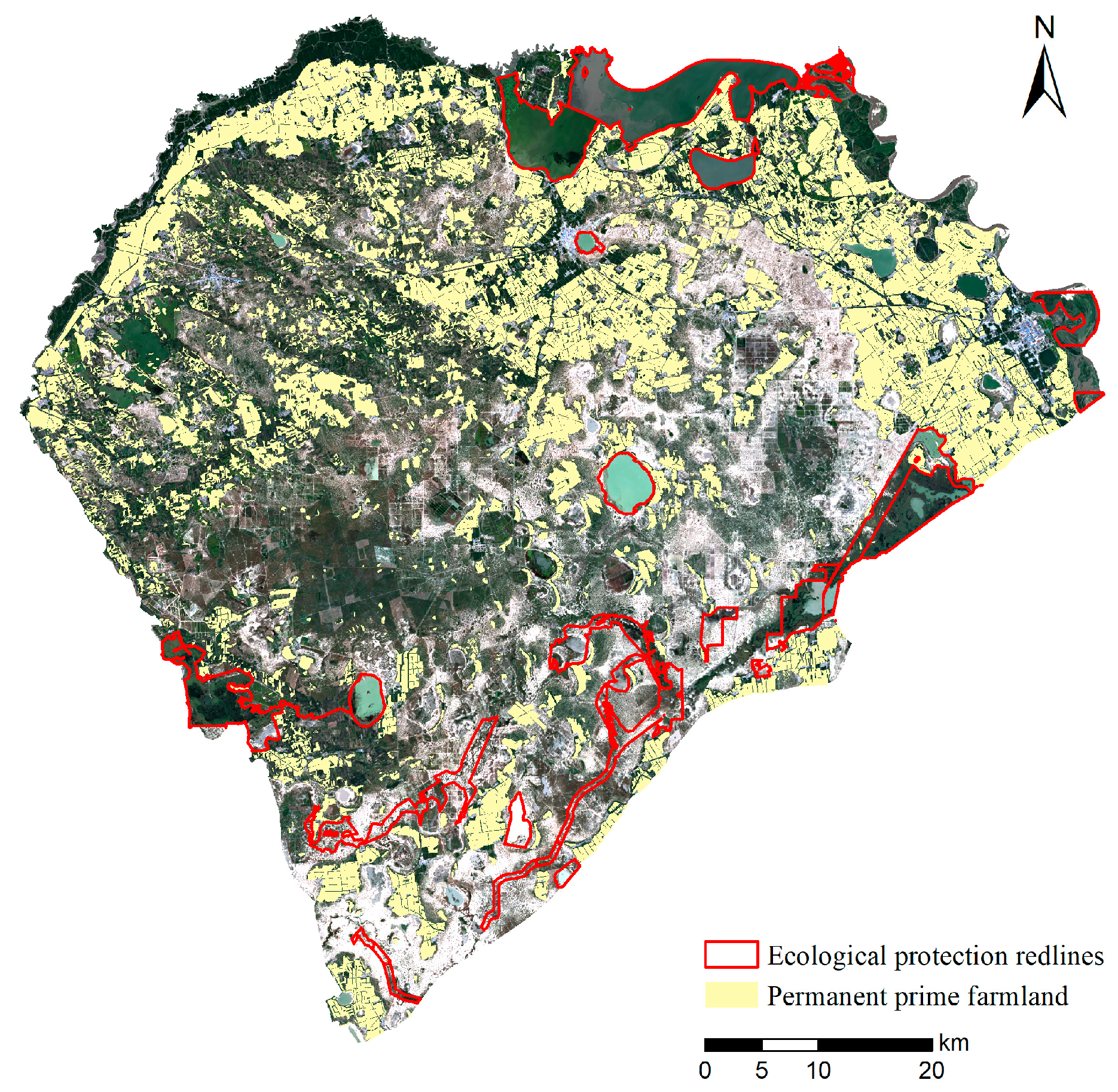
S P B F x 1 1.2 S H P _ 1
( S P B F x 1 1.1 S 2020 _ 1 )
The cultivated land area is not less than the area of permanent prime farmland in the study area, and not more than 1.2 times the cultivated land area in the HD scenario (under the EP scenarios, a substantial increase in cultivated land will occupy ecological land, so the area of cultivated land is limited to no more than 1.1 times the 2020 level).
x 2 + x 3 + x 5 + x 6 + x 8 S r e d l i n e The total area of forest, grass land, wetlands, water bodies and other unutilized land is not less than the area of the ecological protection redline in the study area.
0.8 S 2020 _ 4 x 4 1.18 S 2020 _ 4 According to the Master Plan for the Territorial Space of Da’an City (2021–2035), the area of construction land should not be higher than 1.18 times the 2020 level.
0.8 S H D _ i x i 1.2 S H D _ i According to relevant studies [33,37], and taking into account the actual situation in the study area, the area of each land type should be based on the HD scenario, with a fluctuation range of no more than 20%.
Table 4. Carbon emission coefficient and carbon storage density for land use types (unit: t/grid).
x 1 x 2 x 3 x 4 x 5 x 6 x 7 x 8
C E C i 0.0300.0020.1574.2570.0650.06500
C S D i 13.6620.6913.1213.0826.2426.243.103.10
Table 5. Land use quantity in each scenario (Unit: km2).
HDEPLCSD
Cultivated land2740.312497.043046.292996.24
Forest347.42314.09277.94277.94
Grass land228.72274.47182.98210.21
Construction land164.30144.85144.85144.85
Wetland172.04193.79148.92179.21
Water body391.41401.69409.16401.69
Saline-alkali land399.43479.31319.54319.54
Other unutilized land430.32568.70344.26344.26
Total4873.944873.944873.944873.94
Table 6. The growth probability of cultivated land, ecological land, and saline–alkali land and other unutilized land.
ScenarioTypeCultivated LandEcological LandSaline-Alkali Land and Other Unutilized Land
HDCultivated land99.80%0.00%0.20%
Ecological land5.87%94.09%0.04%
Saline-alkali land and other unutilized land31.36%2.07%66.57%
EPCultivated land99.91%0.01%0.08%
Ecological land5.88%93.63%0.49%
Saline-alkali land and other unutilized land10.03%5.99%83.98%
LCCultivated land99.81%0.00%0.19%
Ecological land17.62%82.32%0.06%
Saline-alkali land and other unutilized land43.25%3.57%53.17%
SDCultivated land99.81%0.00%0.19%
Ecological land15.24%84.69%0.07%
Saline-alkali land and other unutilized land41.49%5.34%53.17%
Disclaimer/Publisher’s Note: The statements, opinions and data contained in all publications are solely those of the individual author(s) and contributor(s) and not of MDPI and/or the editor(s). MDPI and/or the editor(s) disclaim responsibility for any injury to people or property resulting from any ideas, methods, instructions or products referred to in the content.

