
Explainability Feature Bands Adaptive Selection for Hyperspectral Image Classification


Abstract
1. Introduction
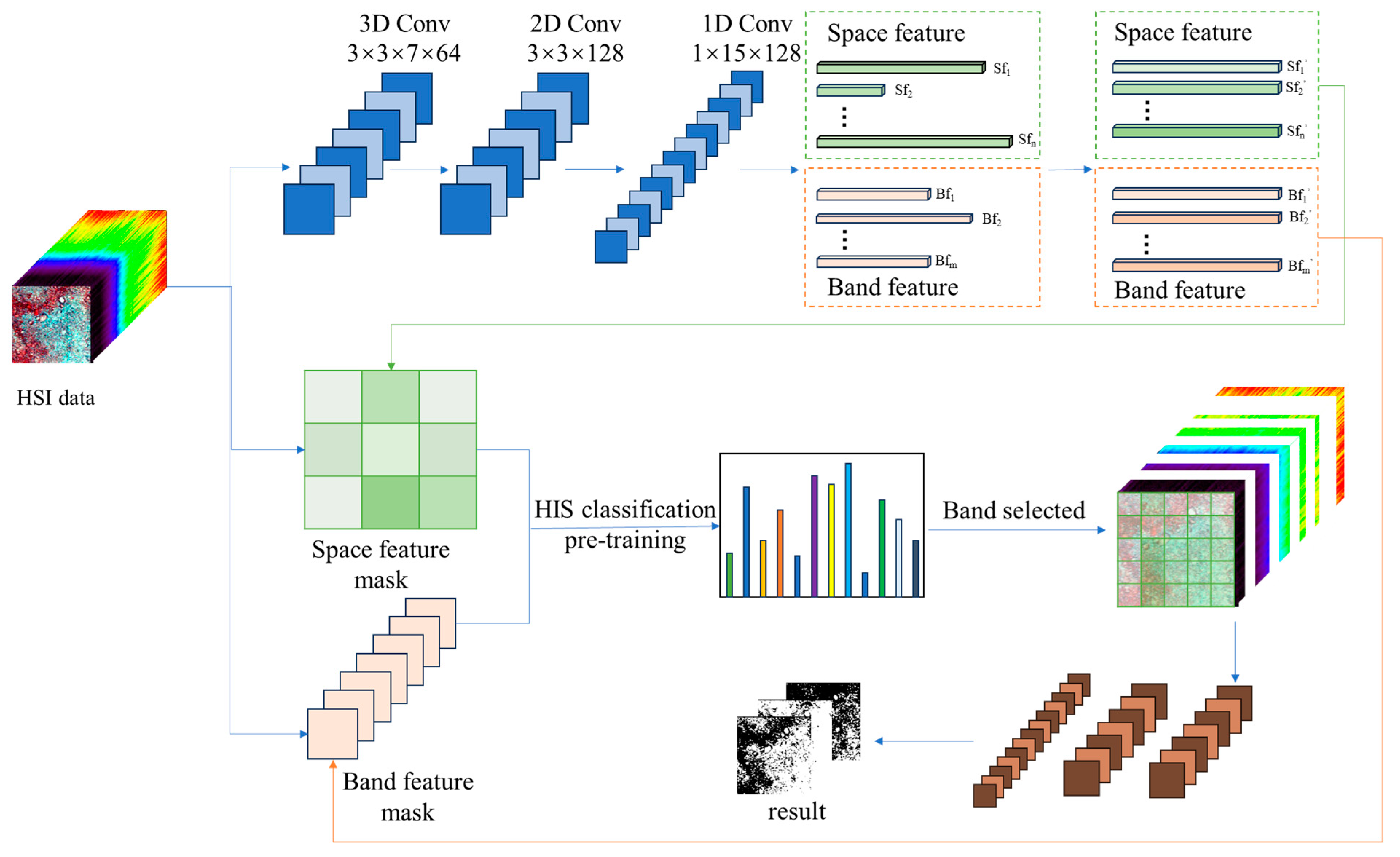
2. Method
2.1. Feature Alignment Modelling
2.2. Self-Attention and Interpretable Model of Feature Features
3. Result
3.1. Experimental Process
- (1)
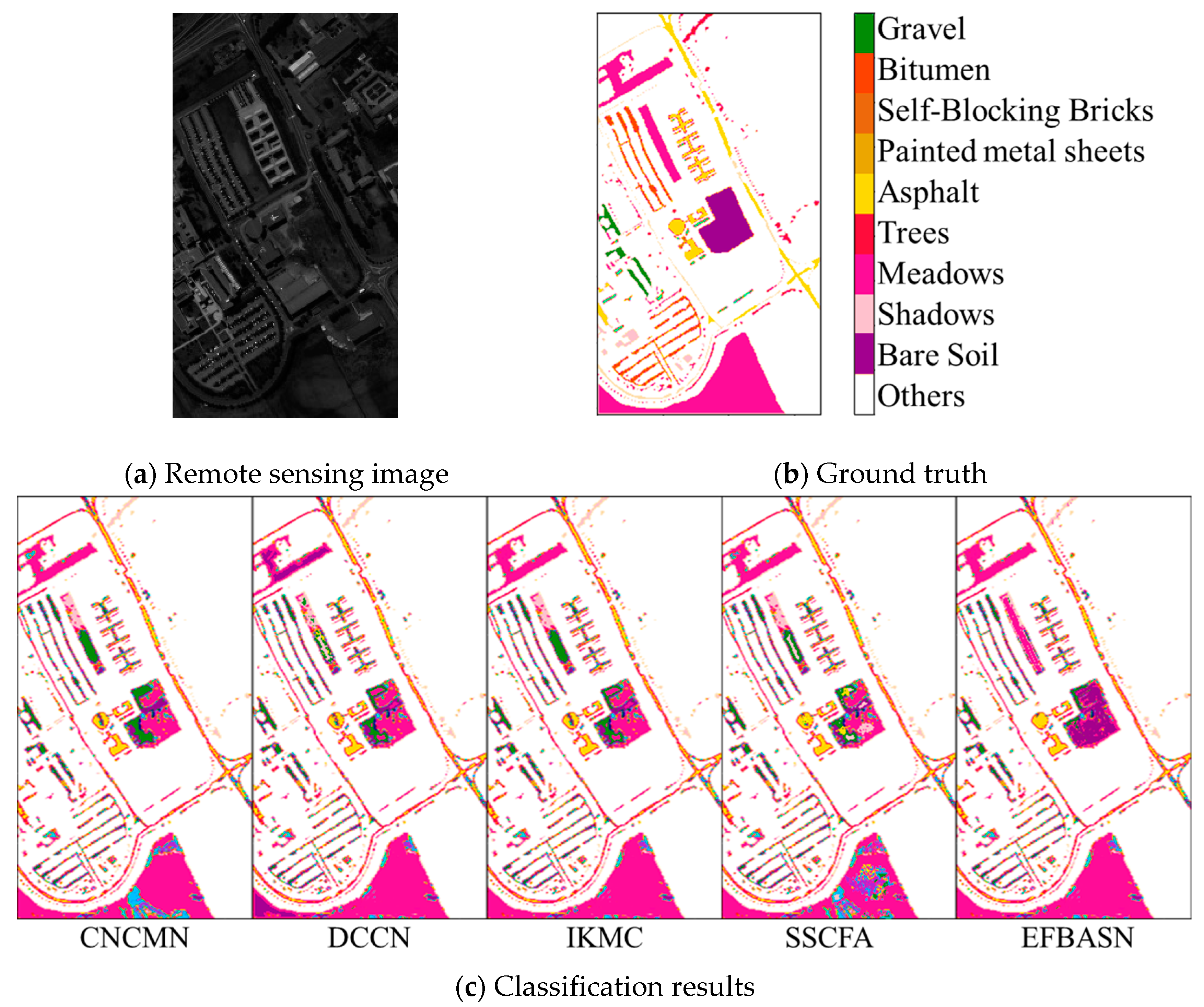
- Pavia University and Pavia Centre datasets. The Pavia University and Pavia Centre datasets were acquired during flights over Pavia in northern Italy, both taken by the ROSIS sensor, in the spectral range 0.430–0.86 µm. The Pavia University is used for training with 103 bands, size 610 × 340, with 9 categories of features, including asphalt roads, metal plates, pastures, etc. Pavia Centre is 1096 × 715 in size and is used for training with 102 bands, also with 9 classifications of features, including trees, asphalt roads, and other features.
- (2)
- Washington DC dataset. The Washington DC dataset is an aerial hyperspectral image over the Washington Mall acquired by the Hydice sensor, with a data size of 1280 × 307 and a spectral range of 191 bands from 0.4 to 2.4 µm. Feature classes include streets, grass, water, gravel paths, trees, shadows, and roofs.
- (3)
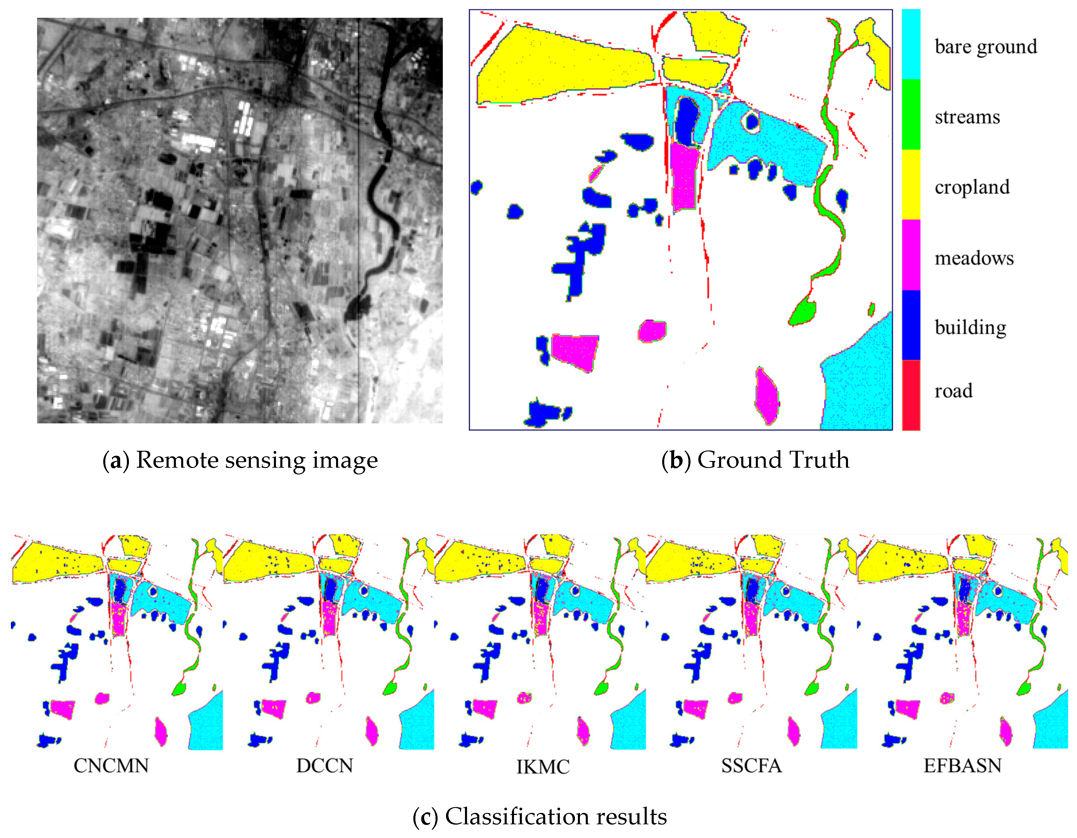
- GF-5 dataset. The GF-5 dataset is an aerospace hyperspectral image of an area over Beijing acquired by the visible short-wave infrared hyperspectral camera on board the GF-5 satellite, with a data size of 301 × 301 and a spectral range of 180 bands from 0.4 to 2.5 µm. The feature categories include grassland, roads, etc. A comprehensive comparison of the basic information of the four hyperspectral datasets is shown in Table 1.
3.2. Comparison Experiment Setup
4. Discussion
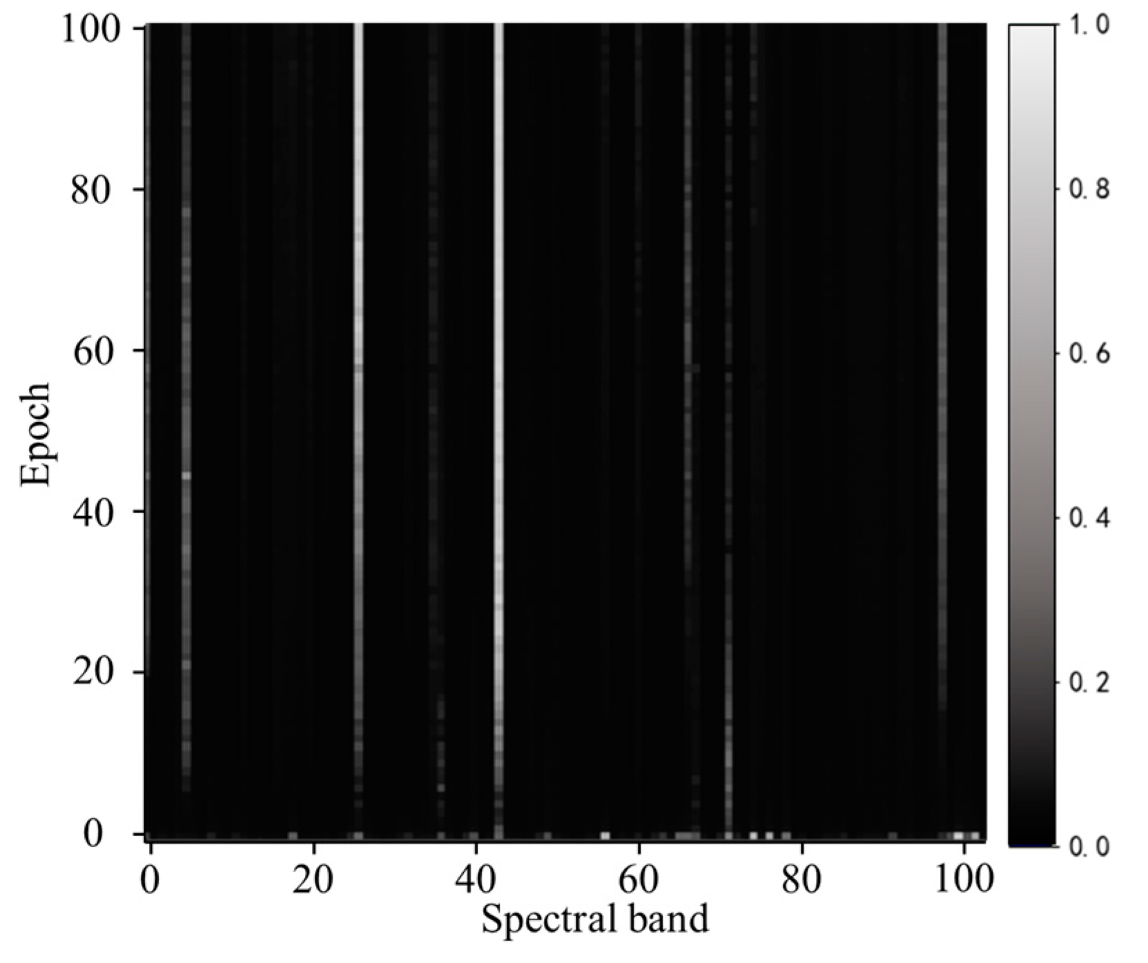
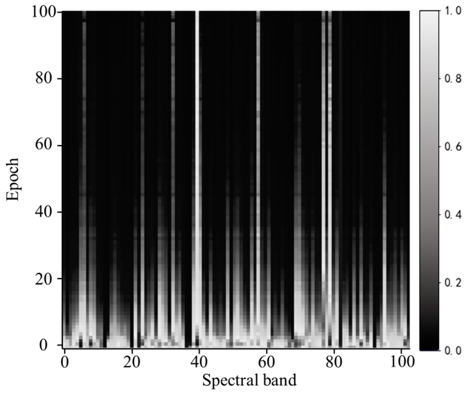
4.1. Comparative Analysis of Interpretable Results
4.2. Comparative Analysis of Classification Results
4.3. Ablation Experiments and Analysis of Results
5. Conclusions
Author Contributions
Funding
Data Availability Statement
Conflicts of Interest
References
- Wang, C.; Huang, J.; Lv, M.; Du, H.; Wu, Y.; Qin, R. A local enhanced mamba network for hyperspectral image classification. Int. J. Appl. Earth Obs. Geoinf. 2024, 133, 104092. [Google Scholar] [CrossRef]
- Jiang, Y.; Zhang, Z.; Zhang, C.; Zhou, H.; Ma, Q.; Zhong, C. S2WaveNet: A novel spectral–spatial wave network for hyperspectral image classification. Int. J. Appl. Earth Obs. Geoinf. 2024, 128, 103754. [Google Scholar] [CrossRef]
- Zhang, X.; Sun, Y.; Qi, W. Hyperspectral Image Classification Based on Extended Morphological Attribute Profiles and Abundance Information. In Proceedings of the 2018 9th Workshop on Hyperspectral Image and Signal Processing: Evolution in Remote Sensing, Amsterdam, The Netherlands, 23–26 September 2018; pp. 1–5. [Google Scholar]
- He, Z.; Xia, K.; Ghamisi, P.; Hu, Y.; Fan, S.; Zu, B. HyperViTGAN: Semisupervised Generative Adversarial Network with Transformer for Hyperspectral Image Classification. IEEE J. Sel. Top. Appl. Earth Obs. Remote Sens. 2022, 15, 6053–6068. [Google Scholar] [CrossRef]
- Paoletti, M.; Haut, J.; Plaza, J.; Plaza, A. Neighboring Region Dropout for Hyperspectral Image Classification. IEEE Geosci. Remote Sens. Lett. 2020, 17, 1032–1036. [Google Scholar] [CrossRef]
- He, N.; Paoletti, M.; Haut, J.; Fang, L.; Li, S.; Plaza, A.; Plaza, J. Feature Extraction with Multiscale Covariance Maps for Hyperspectral Image Classification. IEEE Trans. Geosci. Remote Sens. 2019, 57, 755–769. [Google Scholar] [CrossRef]
- Guo, Z.; Xin, J.; Wang, N.; Li, J.; Gao, X. External-Internal Attention for Hyperspectral Image Super-Resolution. IEEE Trans. Geosci. Remote Sens. 2022, 60, 1–14. [Google Scholar] [CrossRef]
- Zhong, Z.; Li, J.; Luo, Z.; Chapman, M. Spectral–Spatial Residual Network for Hyperspectral Image Classification: A 3-D Deep Learning Framework. IEEE Trans. Geosci. Remote Sens. 2018, 56, 847–858. [Google Scholar] [CrossRef]
- Hong, D.; Han, Z.; Yao, J.; Gao, L.; Zhang, B.; Plaza, A.; Chanussot, J. SpectralFormer: Rethinking hyperspectral image classification with transformers. IEEE Trans. Geosci. Remote Sens. 2022, 60, 5518615. [Google Scholar] [CrossRef]
- Zhang, Q.; Zhu, S.C. Visual interpretability for deep learning: A survey. Front. Inf. Technol. Electron. Eng. 2018, 19, 27–39. [Google Scholar] [CrossRef]
- Zhao, J.; Tian, S.; Geiß, C.; Wang, L.; Zhong, Y.; Taubenbock, H. Spectral-Spatial Classification Integrating Band Selection for Hyperspectral Imagery with Severe Noise Bands. IEEE J. Sel. Top. Appl. Earth Obs. Remote Sens. 2020, 13, 1597–1609. [Google Scholar] [CrossRef]
- Samek, W.; Montavon, G.; Lapuschkin, S.; Anders, C.J.; Muller, K.-R. Explaining Deep Neural Networks and Beyond: A Review of Methods and Applications. Proc. IEEE 2021, 109, 247–278. [Google Scholar] [CrossRef]
- Zeiler, M.; Fergus, R. Visualizing and Understanding Convolutional Networks. European Conference on Computer Vision; Springer: Cham, Switzerland, 2014; pp. 818–833. [Google Scholar]
- Aksoy, S.; Sertel, E.; Roscher, R.; Tanik, A.; Hamzehpour, N. Assessment of soil salinity using explainable machine learning methods and Landsat 8 images. Int. J. Appl. Earth Obs. Geoinf. 2024, 130, 103879. [Google Scholar] [CrossRef]
- Ishikawa, S.-N.; Todo, M.; Taki, M.; Uchiyama, Y.; Matsunaga, K.; Lin, P.; Ogihara, T.; Yasui, M. Example-based explainable AI and its application for remote sensing image classification. Int. J. Appl. Earth Obs. Geoinf. 2023, 118, 103215. [Google Scholar] [CrossRef]
- Zaigrajew, V.; Baniecki, H.; Tulczyjew, L.; Wijata, A.M.; Nalepa, J.; Longépé, N.; Biecek, P. Red Teaming Models for Hyperspectral Image Analysis Using Explainable AI. arXiv 2024, arXiv:2403.08017. [Google Scholar]
- Zhong, S.; Chang, C.; Li, J.; Shang, X.; Chen, S.; Song, M.; Zhang, Y. Class Feature Weighted Hyperspectral Image Classification. IEEE J. Sel. Top. Appl. Earth Obs. Remote Sens. 2019, 12, 4728–4745. [Google Scholar] [CrossRef]
- Sun, K.; Geng, X.; Ji, L. A New Sparsity-Based Band Selection Method for Target Detection of Hyperspectral Image. IEEE Geosci. Remote Sens. Lett. 2014, 12, 329–333. [Google Scholar]
- Qing, Y.; Liu, W.; Feng, L.; Gao, W. Improved transformer net for hyperspectral image classification. Remote Sens. 2021, 13, 2216. [Google Scholar] [CrossRef]
- Porta, C.; Bekit, A.; Lampe, B.; Chang, C. Hyperspectral Image Classification via Compressive Sensing. IEEE Trans. Geosci. Remote Sens. 2019, 57, 8290–8303. [Google Scholar] [CrossRef]
- Shao, Y.; Lan, J.; Niu, B. Dual-Channel Networks with Optimal-Band Selection Strategy for Arbitrary Cropped Hyperspectral Images Classification. IEEE Geosci. Remote Sens. Lett. 2022, 19, 1–5. [Google Scholar] [CrossRef]
- Guo, Y.; Xiao, Y.; Hao, F.; Zhang, X.; Chen, J.; de Beurs, K.; He, Y.; Fu, Y.H. Comparison of different machine learning algorithms for predicting maize grain yield using UAV-based hyperspectral images. Int. J. Appl. Earth Obs. Geoinf. 2023, 124, 103528. [Google Scholar] [CrossRef]
- Liu, J.; Lan, J.; Zeng, Y. GL-Pooling: Global–Local Pooling for Hyperspectral Image Classification. IEEE Geosci. Remote Sens. Lett. 2023, 20, 5509305. [Google Scholar] [CrossRef]
- Guo, X.; Hou, B.; Yang, C.; Ma, S.; Ren, B.; Wang, S.; Jiao, L. Visual explanations with detailed spatial information for remote sensing image classification via channel saliency. Int. J. Appl. Earth Obs. Geoinf. 2023, 118, 103244. [Google Scholar] [CrossRef]
- Xin, Z.; Li, Z.; Xu, M.; Wang, L.; Ren, G.; Wang, J.; Hu, Y. Feature disentanglement based domain adaptation network for cross-scene coastal wetland hyperspectral image classification. Int. J. Appl. Earth Obs. Geoinf. 2024, 129, 103850. [Google Scholar] [CrossRef]
- Haut, J.; Paoletti, M.; Plaza, J.; Plaza, A.; Li, J. Visual Attention-Driven Hyperspectral Image Classification. IEEE Trans. Geosci. Remote Sens. 2019, 57, 8065–8080. [Google Scholar] [CrossRef]
- Chang, C.; Du, Q.; Sun, T.; Althouse, M.L.G. A Joint Band Prioritization and Band-Decorrelation Approach to Band Selection for Hyperspectral Image Classification. IEEE Trans. Geosci. Remote Sens. 1999, 37, 2631–2641. [Google Scholar] [CrossRef]
- Wang, L.; Wang, Q. Fast spatial-spectral random forests for thick cloud removal of hyperspectral images. Int. J. Appl. Earth Obs. Geoinf. 2022, 112, 102916. [Google Scholar] [CrossRef]
- He, X.; Chen, Y.; Lin, Z. Spatial–spectral transformer for hyperspectral image classification. Remote Sens. 2021, 13, 498. [Google Scholar] [CrossRef]
- Sun, L.; Zhao, G.; Zheng, Y.; Wu, Z. Spectral–spatial feature tokenization transformer for hyperspectral image classification. IEEE Trans. Geosci. Remote Sens. 2022, 60, 5522214. [Google Scholar] [CrossRef]
- Shu, Z.; Wang, Y.; Yu, Z. Dual attention transformer network for hyperspectral image classification. Eng. Appl. Artif. Intell. 2024, 127, 107351. [Google Scholar] [CrossRef]
- Gong, M.; Zhang, M.; Yuan, Y. Unsupervised Band Selection Based on Evolutionary Multiobjective Optimization for Hyperspectral Images. IEEE Trans. Geosci. Remote Sens. 2015, 54, 544–557. [Google Scholar] [CrossRef]
- Cai, Y.; Liu, X.; Cai, Z. BS-Nets: An End-to-End Framework for Band Selection of Hyperspectral Image. IEEE Trans. Geosci. Remote Sens. 2019, 58, 1969–1984. [Google Scholar] [CrossRef]
- Ben Hamida, A.; Benoit, A.; Lambert, P.; Ben Amar, C. 3-D Deep Learning Approach for Remote Sensing Image Classification. IEEE Trans. Geosci. Remote Sens. 2018, 56, 4420–4434. [Google Scholar] [CrossRef]
- Paoletti, M.E.; Haut, J.M.; Fernandez-Beltran, R.; Plaza, J.; Plaza, A.J.; Pla, F. Deep Pyramidal Residual Networks for Spectral–Spatial Hyperspectral Image Classification. IEEE Trans. Geosci. Remote Sens. 2019, 57, 740–754. [Google Scholar] [CrossRef]
- Shi, K.; Liu, Q.; Zheng, Z.; Xiao, L. Efficient Implementation for Composite CNN-Based HSI Classification Algorithm with Huawei Ascend Framework. In Proceedings of the 2023 13th WHISPERS, Athens, Greece, 19 February 2023; pp. 1–5. [Google Scholar]
- Yu, H.; Zhang, H.; Liu, Y.; Zheng, K.; Xu, Z.; Xiao, C. Dual-Channel Convolution Network with Image-Based Global Learning Framework for Hyperspectral Image Classification. IEEE Geosci. Remote Sens. Lett. 2022, 19, 6005705. [Google Scholar] [CrossRef]
- Goud, O.S.C.; Sarma, T.H.; Bindu, C.S. Improved K-Means Clustering Algorithm for Band Selection in Hyperspectral Images. In Proceedings of the 2023 International Conference on Electrical, Electronics, Communication and Computers (ELEXCOM), Roorkee, India, 26–27 August 2023; pp. 1–6. [Google Scholar]
- Li, W.; Yang, Y.; Zhang, M.; Mi, P.; Xiao, Z.; Xiang, J. Deep Spatial-Spectral Feature Extraction Network for Hyperspectral Image Classification. In Proceedings of the 2024 43rd Chinese Control Conference (CCC), Kunming, China, 28–31 July 2024; pp. 7955–7960. [Google Scholar]
- Sun, W.; Du, Q. Hyperspectral Band Selection: A Review. IEEE Geosci. Remote Sens. Mag. 2019, 7, 118–139. [Google Scholar] [CrossRef]


| Dataset | Pavia University | Pavia Centre | Washington DC | GF-5 |
|---|---|---|---|---|
| Size | 610 × 340 | 1096 × 715 | 1280 × 307 | 301 × 301 |
| Band | 103 | 102 | 191 | 180 |
| Class | 9 | 9 | 7 | 6 |
| Number of Marker Pixels | 42,776 | 7456 | 19,204 | 3649 |
| spectral range (μm) | 0.43–0.86 | 0.43–0.86 | 0.4–2.4 | 0.4–2.5 |
| Class Name | CNCMN | DCCN | IKMC | SSCFA | EFBASN |
|---|---|---|---|---|---|
| Gravel | 93.84 | 95.77 | 92.66 | 95.96 | 99.46 |
| Bitumen | 98.76 | 98.22 | 96.88 | 99.08 | 99.38 |
| Self-Blocking Bricks | 95.97 | 99.14 | 97.81 | 99.08 | 99.45 |
| Painted metal sheets | 98.08 | 96.12 | 90.20 | 93.47 | 98.22 |
| Asphalt | 97.25 | 96.96 | 97.20 | 98.20 | 98.85 |
| Trees | 92.07 | 97.72 | 94.21 | 97.15 | 97.16 |
| Meadows | 91.94 | 95.03 | 96.34 | 90.02 | 95.92 |
| Shadows | 87.09 | 91.73 | 91.47 | 95.95 | 94.24 |
| Bare Soil | 84.04 | 87.06 | 80.88 | 81.65 | 95.88 |
| OA | 93.12 | 95.25 | 93.18 | 94.48 | 97.68 |
| AA | 93.22 | 95.30 | 93.07 | 94.50 | 97.61 |
| 93.20 | 95.28 | 93.15 | 94.49 | 97.63 |
| Class Name | CNCMN | DCCN | IKMC | SSCFA | EFBASN |
|---|---|---|---|---|---|
| Bitumen | 93.88 | 94.76 | 94.96 | 95.34 | 96.97 |
| Tiles | 88.76 | 84.31 | 85.76 | 88.68 | 89.32 |
| Asphalt | 95.97 | 98.14 | 94.44 | 89.45 | 99.45 |
| Self-Blocking Bricks | 80.44 | 80.93 | 81.33 | 82.54 | 83.03 |
| Bare soil | 90.56 | 91.55 | 90.08 | 91.38 | 92.78 |
| Trees | 90.98 | 91.39 | 91.55 | 91.03 | 91.86 |
| Meadows | 78.66 | 83.68 | 80.79 | 81.62 | 90.63 |
| Shadows | 80.78 | 80.66 | 80.48 | 80.43 | 80.98 |
| Water | 76.04 | 96.06 | 84.58 | 80.35 | 97.88 |
| OA | 86.32 | 88.93 | 87.07 | 86.78 | 91.41 |
| AA | 86.23 | 89.05 | 87.10 | 86.75 | 91.43 |
| 86.20 | 89.00 | 87.09 | 86.77 | 91.42 |
| Class Name | CNCMN | DCCN | IKMC | SSCFA | EFBASN |
|---|---|---|---|---|---|
| Water | 79.53 | 83.24 | 84.29 | 85.67 | 98.71 |
| Grass | 79.22 | 78.93 | 78.98 | 87.34 | 93.77 |
| Roof | 89.88 | 89.63 | 90.36 | 90.55 | 91.54 |
| Road | 92.79 | 93.04 | 93.53 | 92.91 | 94.22 |
| Tree | 83.25 | 81.67 | 81.81 | 82.53 | 87.79 |
| Path | 77.31 | 76.29 | 74.69 | 75.91 | 81.33 |
| Shadow | 81.22 | 82.03 | 81.97 | 80.93 | 86.61 |
| OA | 83.33 | 83.52 | 83.64 | 85.15 | 90.60 |
| AA | 83.31 | 83.54 | 83.66 | 85.12 | 90.56 |
| 83.32 | 83.53 | 83.65 | 85.13 | 90.58 |
| Class Name | CNCMN | DCCN | IKMC | SSCFA | EFBASN |
|---|---|---|---|---|---|
| bare ground | 96.53 | 97.78 | 98.05 | 97.51 | 98.79 |
| streams | 99.54 | 99.35 | 99.89 | 99.91 | 99.93 |
| cropland | 98.90 | 97.69 | 98.40 | 97.93 | 98.88 |
| meadows | 96.73 | 97.21 | 97.16 | 97.51 | 97.29 |
| building | 97.29 | 98.62 | 97.78 | 97.89 | 97.51 |
| road | 92.79 | 93.26 | 93.58 | 93.93 | 94.98 |
| OA | 96.98 | 97.28 | 97.51 | 97.42 | 97.86 |
| AA | 96.96 | 97.31 | 97.47 | 97.44 | 97.89 |
| 96.97 | 97.30 | 97.48 | 97.43 | 97.88 |
| Case | Space Feature Self-Attention | Band Feature Self-Attention | Band Select | OA | AA |
|---|---|---|---|---|---|
| 1 | × | × | × | 68.32 | 59.03 |
| 2 | √ | × | × | 82.49 | 79.51 |
| 3 | × | √ | × | 90.67 | 87.84 |
| 4 | × | × | √ | 85.10 | 84.96 |
| 5 | √ | √ | √ | 97.86 | 97.89 |
Disclaimer/Publisher’s Note: The statements, opinions and data contained in all publications are solely those of the individual author(s) and contributor(s) and not of MDPI and/or the editor(s). MDPI and/or the editor(s) disclaim responsibility for any injury to people or property resulting from any ideas, methods, instructions or products referred to in the content. |
© 2025 by the authors. Licensee MDPI, Basel, Switzerland. This article is an open access article distributed under the terms and conditions of the Creative Commons Attribution (CC BY) license (https://creativecommons.org/licenses/by/4.0/).
Share and Cite
Liu, J.; Lan, J.; Zeng, Y.; Luo, W.; Zhuang, Z.; Zou, J. Explainability Feature Bands Adaptive Selection for Hyperspectral Image Classification. Remote Sens. 2025, 17, 1620. https://doi.org/10.3390/rs17091620
Liu J, Lan J, Zeng Y, Luo W, Zhuang Z, Zou J. Explainability Feature Bands Adaptive Selection for Hyperspectral Image Classification. Remote Sensing. 2025; 17(9):1620. https://doi.org/10.3390/rs17091620
Chicago/Turabian StyleLiu, Jirui, Jinhui Lan, Yiliang Zeng, Wei Luo, Zhixuan Zhuang, and Jinlin Zou. 2025. "Explainability Feature Bands Adaptive Selection for Hyperspectral Image Classification" Remote Sensing 17, no. 9: 1620. https://doi.org/10.3390/rs17091620
APA StyleLiu, J., Lan, J., Zeng, Y., Luo, W., Zhuang, Z., & Zou, J. (2025). Explainability Feature Bands Adaptive Selection for Hyperspectral Image Classification. Remote Sensing, 17(9), 1620. https://doi.org/10.3390/rs17091620