Abstract
Object detection is essential for precision agriculture applications like automated plant counting, but the minimum dataset requirements for effective model deployment remain poorly understood for arable crop seedling detection on orthomosaics. This study investigated how much annotated data is required to achieve standard counting accuracy (R2 = 0.85) for maize seedlings across different object detection approaches. We systematically evaluated traditional deep learning models requiring many training examples (YOLOv5, YOLOv8, YOLO11, RT-DETR), newer approaches requiring few examples (CD-ViTO), and methods requiring zero labeled examples (OWLv2) using drone-captured orthomosaic RGB imagery. We also implemented a handcrafted computer graphics algorithm as baseline. Models were tested with varying training sources (in-domain vs. out-of-distribution data), training dataset sizes (10–150 images), and annotation quality levels (10–100%). Our results demonstrate that no model trained on out-of-distribution data achieved acceptable performance, regardless of dataset size. In contrast, models trained on in-domain data reached the benchmark with as few as 60–130 annotated images, depending on architecture. Transformer-based models (RT-DETR) required significantly fewer samples (60) than CNN-based models (110–130), though they showed different tolerances to annotation quality reduction. Models maintained acceptable performance with only 65–90% of original annotation quality. Despite recent advances, neither few-shot nor zero-shot approaches met minimum performance requirements for precision agriculture deployment. These findings provide practical guidance for developing maize seedling detection systems, demonstrating that successful deployment requires in-domain training data, with minimum dataset requirements varying by model architecture.
1. Introduction
1.1. Arable Crop Plant Counting by Object Detection
Plant counting is a critical operation in precision agriculture, plant breeding, and agronomical evaluation. Accurate plant detection and counting in agricultural applications serves multiple critical functions:
- Crop Establishment Assessment: Early-season seedling counts determine whether or not replanting is necessary, directly affecting yield potential and economic returns [1].
- Precision Agriculture: Individual plant locations enable variable-rate application of inputs (fertilizers, pesticides) and selective harvesting, reducing costs and environmental impact [2].
- Plant Breeding Programs: Automated counting accelerates phenotyping workflows, enabling evaluation of larger populations and more traits [3].
- Insurance and Compliance: Standardized counting methods support crop insurance assessments and regulatory compliance for agricultural subsidies [4].
- Research Applications: Consistent counting methods enable meta-analyses across studies and reproducible research in agronomy [5].
Traditionally performed manually, this labor-intensive task is increasingly automated through computer vision algorithms.
To validate any counting method, establishing a performance benchmark is essential. Such benchmarks can derive from manual counting accuracy, international standards, or comparison with established methods. According to the European Plant Protection Organization, acceptable plant counting methods must achieve a coefficient of determination (R2) of 0.85 when compared to manual counting [5], corresponding to a Root Mean Square Error (RMSE) of approximately 0.39. This same benchmark (R2 = 0.85) is widely recognized in the scientific literature [6].
In agricultural applications specifically, object detection offers advantages over regression-based counting methods. Studies show object detection not only achieves superior accuracy [6] but also provides geographical plant coordinates when applied to georeferenced orthomosaics, rather than just density estimates. The validation of this ability relies on metrics such as Intersection over Union (), Average Precision (), and Average Recall [7] rather than on the coefficient of determination.
Georeferenced orthomosaics—created through aerial photogrammetry from overlapping images with Ground Control Points (GCPs) [8]—are particularly valuable for agricultural counting applications. Their fixed scale and orientation to geographical coordinates simplify object detection by providing consistent object sizes and eliminating perspective distortion. However, georeferenced orthomosaics also present certain limitations. Georeferencing errors due to low-quality or insufficient GCPs, or reliance on onboard GNSS/IMU systems, can significantly reduce spatial accuracy. This is particularly the case in datasets derived from unmanned aerial vehicles [9,10]. Moreover, distortions may persist in areas with high relief or vegetation canopy variability if digital elevation models are inadequately detailed [11,12]. Finally, computational demand and processing time during photogrammetric reconstruction remain a constraint, particularly for high-resolution or large-area orthomosaics [13].
Like many computer vision tasks in specialized domains, agricultural plant counting suffers from data scarcity [14]. Public datasets are limited and often lack critical information like orthorectification parameters or precise scale information. To focus our investigation, we selected grain maize seedlings (Zea mays L.) at the V3–V5 growth stage [15] as our case study, as this crop is well represented in both the scientific literature [16,17] and public repositories [18,19].
Maize, the world’s highest-production crop [20], offers ideal characteristics for object detection at this growth stage. Its regular planting pattern with defined inter-row and intra-row spacing, minimal overlapping, and distinctive appearance makes it suitable for automated counting. These characteristics are shared by other row crops like sunflower (Helianthus annuus L.) and sugarbeet (Beta vulgaris L.), potentially making our findings applicable to a broader range of agricultural scenarios [21].
1.2. Evolution of Object Detection Methods
The broader field of object detection has evolved from non-machine learning methods, here named Handcrafted (HC) methods, to sophisticated Deep Learning (DL) approaches. Handcrafted methods rely on explicitly programmed rules and traditional computer vision techniques such as color thresholding, edge detection, and morphological operations to identify objects. These approaches require domain expertise to design feature extraction algorithms but offer interpretability and computational efficiency [16,22]. While state-of-the-art detection now relies primarily on DL, HC methods still find application in agricultural contexts [16,23].
Modern DL object detection architectures fall into two main categories: those based on Convolutional Neural Networks (CNNs) [24] like Faster R-CNN [25] and YOLO [26], and those employing Transformer architectures [27] like DETR [28], or hybrid approaches combining both paradigms. The fundamental difference lies in how images are processed—CNNs use grid-based convolutions while Transformers process image patches using attention mechanisms [29].
On standard computer vision benchmarks like COCO [7] and ImageNet [30], Transformer-based approaches generally outperform CNN-based models in accuracy [31]. However, in agricultural applications specifically, CNN-based architectures like YOLO variants remain widely used due to their efficiency with smaller images and lower computational requirements [32,33]. For agricultural deployment with limited training data, Transformer-based models may offer advantages in fine-tuning scenarios [34,35].
For our comparative analysis of agricultural object detection approaches, we selected representative architectures from both paradigms. From the CNN family, we chose YOLOv5 and YOLOv8 due to their widespread agricultural adoption [33]. From Transformer-mixed architectures, we selected RT-DETR [36] and YOLO11 [37], which demonstrate state-of-the-art performance on standard benchmarks.
1.3. Data-Efficient Detection Methods
A critical challenge in agricultural object detection is the high cost of data annotation. Recently, emerging paradigms like zero-shot and few-shot object detection offer potential solutions by reducing or eliminating annotation requirements. These approaches differ fundamentally from traditional “many-shot” detectors in their data needs.
In few-shot detection, models learn to identify objects from minimal examples—often just 1–30 annotated instances (or “shots”). These methods typically leverage feature transfer or meta-learning [38] to generalize from limited data. The agricultural potential of such approaches is significant, as they could drastically reduce annotation burden for new crop varieties or growth stages.
Zero-shot detection represents the extreme case where models detect novel objects without any labeled examples by exploiting semantic relationships or contextual information learned from other classes [39]. State-of-the-art zero-shot detectors include YOLO-World [40], OWLv2 [41], and Grounding DINO [42].
While these data-efficient approaches show promise in general computer vision tasks, their effectiveness for agricultural applications remains largely unexplored. For maize seedling detection specifically, only two studies have investigated few-shot methods [43,44], with neither achieving benchmark performance or clearly specifying shot counts. No studies have yet evaluated zero-shot detection for maize seedling counting.
1.4. Dataset Requirements for Agricultural Object Detection
While general object detection benchmarks provide standardized evaluation, they poorly represent agricultural conditions. Numerous studies have addressed plant detection in field settings [17,45,46], but few have systematically investigated minimum dataset requirements for robust performance [16,47].
This knowledge gap creates significant challenges for practitioners who must determine how much data to collect and annotate for effective deployment. The agricultural domain’s unique characteristics—variable environment, specific plant phenotypes, and orthomosaic imagery—may substantially alter data requirements compared to general computer vision tasks.
General deep learning principles suggest model performance correlates strongly with training data quantity [48] and quality [49]. These relationships can be modeled using empirical approaches [50,51]. Other factors affecting minimum dataset requirements include model architecture [52], backbone selection [53], and data augmentation strategies [54].
The most critical factor, however, appears to be dataset source. Studies consistently show that using in-domain data (from the same distribution as the inference target) dramatically improves accuracy while reducing required dataset size compared to out-of-distribution training [16,47]. This finding has profound implications for agricultural deployment scenarios.
1.5. Study Aim
This study aims to establish the minimum dataset requirements for accurate maize seedling detection in georeferenced orthomosaics across different object detection paradigms. Here, the dataset size and quality are respectively defined as the amount of annotated images in the training set and the accuracy of the annotations. In particular, the annotation quality is defined as the percentage of correct annotations relative to the total ground truth annotations present in each image, with 100% representing perfect annotations where every plant is correctly identified and bounded. For example, if an image contains 10 plants and the annotator correctly identifies and bounds 8 of them, the annotation quality for that image would be 80%. To simulate varying annotation quality levels, we systematically removed a percentage of existing annotations from our complete ground truth dataset, effectively simulating scenarios where human annotators miss a certain proportion of plants due to factors such as time constraints, fatigue, or challenging visual conditions. This approach allows us to evaluate how robust different models are to incomplete annotations, which is a common real-world scenario in agricultural applications where exhaustive annotation can be prohibitively expensive or time-consuming. Specifically, we investigate the following:
- How training data source (in-domain vs. out-of-distribution) affects required dataset size
- Minimum dataset size needed to achieve benchmark performance (R2 = 0.85) for different model architectures
- Minimum annotation quality required to maintain benchmark performance
- Whether or not newer few-shot and zero-shot approaches can meet agricultural performance standards with reduced annotation requirements
- The potential role of handcrafted methods in modern deep learning pipelines
By systematically varying training dataset size (10–150 images), annotation quality (10–100%), and evaluating diverse architectures (CNN-based, Transformer-based, few-shot, and zero-shot), we provide comprehensive guidance for implementing efficient maize seedling detection systems. Our findings establish empirical relationships between dataset characteristics and model performance, offering practical insights for optimizing the annotation effort versus detection performance trade-off in agricultural object detection.
2. Materials and Methods
2.1. Datasets
The datasets used in this study to train the object detection models for maize seedling counting are nadiral or supposedly nadiral images of maize seedlings at the V3–V5 growth stage, or estimated so. The V3–V5 growth stage is defined by the BBCH scale as the stage where the third to fifth leaf is unfolded and the plant is 15–30 cm tall [15].
This study uses two dataset sources as training sets: the Out-of-Distribution (OOD) dataset and the In-Domain (ID) dataset. The ID datasets are from the same source as the testing dataset, while the OOD datasets are not. The OOD datasets are composed of images from scientific literature [16,55] and from internet repositories [18,19]. The ID datasets were collected during this study. This ID dataset creation consisted of capturing nadiral images of three study areas with a Phantom 4 Pro v2.0 (DJI, Shenzhen, China) drone equipped with its default series RGB camera at about 10 m above ground for a Ground Sampling Distance (GSD) of 2.7 mm/pixel. The number of images captured depends on the study area size, which was about 2 hectares for the ID_1 location and about 1 ha for the other two. For each location, an orthomosaic was created using photogrammetric software. Bundle adjustment error was estimated as 38 mm using the GCPs surveyed by GNSS operating in VRS-NRTK mode. The orthomosaics were generated with an average GSD of 5 mm/pixel in the WGS84/UTM 32 N reference system. We chose this GSD because it is the minimum GSD that allows the detection of maize seedlings at the V3–V5 growth stage with a nadiral camera [56].
The OOD scientific datasets consist of tiles of georeferenced orthomosaics of maize seedlings from the scientific literature. The OOD internet datasets consist of RGB images of maize seedlings from internet repositories. The ID datasets were collected during this study and consist of tiles of georeferenced orthomosaics of maize seedlings of known scale. The OOD scientific datasets and the ID datasets are composed of tiles of georeferenced orthomosaics of known scale, while the OOD internet datasets are simple RGB images of unknown scale. All the OOD datasets came with annotations, while the ID datasets were manually annotated. The OOD dataset annotations are rectangular bounding boxes centering on an individual plant stem. ID dataset annotation was done during this study by an agronomist by observing the entire orthomosaic in a Geographical Information System (GIS) environment, with the tile grid overlapping the orthomosaic to focus on target tiles without losing the surrounding context, so without losing bordering plants. Annotations were created as squared bounding boxes of a size length equal to the minimum distance between two plants in the row, with each box centered on an individual seedling stem.
Table 1 summarizes the datasets used in this study.

Table 1.
Summary of datasets used in the study.
To make the two types of datasets comparable, we chose to rescale the images to a scale of 0.005 m/pixel where the scale was known (scientific OOD and ID datasets), obtaining orthomosaics of different sizes. All the orthomosaics were then cropped to 224 × 224 pixel tiles. This tile size was selected because at 5 mm/pixel resolution it covers 1.12 × 1.12 m of field area. Given that typical grain maize inter-row distance is 0.75 m, this size enables capturing approximately two rows per tile, which is optimal for row pattern identification in the HC algorithm and provides sufficient context for object detection models [16,55]. This particular image size was also chosen as a standard from AlexNet [58] as it should be compatible with most of the object detection architectures. The annotations were rescaled and cropped where needed. Figure 1 shows a sample for each dataset. Each ID dataset has 20 tiles to be used as the testing dataset, while the other 150 tiles are used as the training dataset.
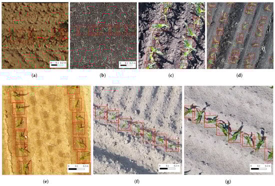
Figure 1.
Image examples taken from each dataset, ground truth bounding boxes are shown in red. (a) DavidEtAl.2021, (b) LiuEtAl.2022, (c) Internet Maize stage V3, (d) Internet Maize stage V5, (e) ID_1, (f) ID_2, (g) ID_3.
2.2. Handcrafted Object Detector
Like other works [16,23,55], we wrote an HC algorithm to obtain annotated tiles from the orthomosaics, basing it on agronomical knowledge and color thresholding. Hue, Saturation, and Value (HSV) color space was used here to threshold the image, to obtain green pixels, but other color spaces can be used. For the execution of this algorithm, the following graphical and agronomical parameters must be set: color minimum and maximum thresholds (color threshold), the minimum and maximum leaf area for the plant (leaf area range), the minimum distance between plants on rows (intra-row distance), and the distance between rows (inter-rows distance). The algorithm is expected to work on the orthomosaics of maize seedlings at the V3–V5 growth stage, with low weed infestation, with rows having roughly the same angle with meridian and distance between them. The algorithm was implemented in Python 3.13.1 using the following packages: numpy (v 1.24.3), torch (v 2.0.1), PyYAML (v 6.0), rasterio (v 1.3.8), shapely (v 2.0.1), fiona (v 1.9.4), scikit-image (v 0.21.0), scikit-learn (v 1.3.0), matplotlib (v 3.7.1). The complete implementation is accessible from https://gist.github.com/SamueleBumbaca/4a227bbe7b78d6be3424899c16c60bb4 (accessed on 20 June 2025).
The algorithm is divided in two sequential parts that form a detection–verification pipeline. The first part, named HC1 Algorithm A1, performs initial plant detection by thresholding pixels within the specified color range, identifying connected regions, and filtering them based on expected leaf area. HC1 outputs region polygons representing potential plants, but typically includes many false positives due to its simple color-based approach. To address this limitation, we implemented a second process named HC2 Algorithm A2 that applies agronomical knowledge of field structure. HC2 filters the HC1 output by verifying that detected plants form proper row patterns with expected intra-row and inter-row spacing. It uses RANSAC [59] to identify the linear alignments of plants and validates that these alignments match expected field geometry (consistent row slope and spacing). Only tiles where HC2 confirms the expected number and arrangement of plants are retained for the final dataset. This two-stage approach enables the automated extraction of high-confidence annotations from the orthomosaics. Complete algorithm pseudocodes are provided in the Appendix A.
2.3. Deep Learning Object Detectors
Many-shot model selection criteria: From the extensive landscape of available object detection architectures, we applied the following selection criteria: (1) widespread adoption in agricultural computer vision applications [33], (2) availability of multiple model sizes to investigate parameter count effects on dataset requirements, (3) representation of different architectural paradigms (CNN-based vs. Transformer-based), (4) consistent implementation framework for fair comparison, and (5) proven performance on small object detection tasks relevant to seedling identification. The many-shot object detectors used in this study include YOLOv5, YOLOv8, RT-DETR, and YOLO11. Each represents distinct architectural approaches to object detection:
- YOLOv5 with model descriptions uses a CSP (Cross Stage Partial) backbone with a PANet neck for feature aggregation, achieving efficient detection through grid-based prediction with multiple anchors per cell. It was selected as the baseline CNN architecture due to its dominance in agricultural applications [33] and extensive use in crop monitoring studies [45,46]. Its CSP backbone with PANet neck provides a well-established reference point for minimum dataset requirements in agricultural contexts.
- YOLOv8 with model descriptions improves upon YOLOv5 by adopting a more efficient C2f block in its backbone, implementing an anchor-free detection head and using a task-specific decoupled head design for better accuracy–speed trade-offs. It represents the next-generation YOLO evolution with anchor-free detection and improved C2f blocks. We included it to evaluate whether or not architectural improvements could reduce dataset requirements compared to YOLOv5, given its reported superior accuracy–efficiency trade-offs [60].
- YOLO11 with model descriptions further refines the architecture with multi-scale deformable attention, improving small object detection—a crucial feature for seedling identification in varied field conditions. It was chosen as the most recent YOLO variant including an attention mechanisms (transformer). This selection allows us to assess whether or not state-of-the-art Transformer-mixed improvements affect minimum dataset requirements for small object detection.
- RT-DETR with model descriptions represents a hybrid approach combining CNN backbones with Transformer decoders, utilizing deformable attention for adaptive feature sampling and parallel prediction heads for real-time performance. Unlike pure CNN-based YOLO variants, RT-DETR’s Transformer components enable the modeling of global relationships between objects. We selected it over pure Transformer models (like DETR) due to its real-time capabilities and proven performance on agricultural datasets [36]. Its inclusion allows direct comparison between CNN-only and hybrid approaches for minimum dataset requirements.
Excluded alternatives and rationale: with model descriptions We deliberately excluded several model families: Faster R-CNN and other two-stage detectors due to their computational overhead and limited agricultural adoption; pure Transformer models like DETR due to prohibitive training requirements for small datasets [28]
We used the Ultralytics implementation for all models as it is open-source [61] and enables consistent parameter tuning across architectures.
All model training and inference were performed on a workstation equipped with an Intel(R) Xeon(R) CPU E5-2670 v3 @ 2.30 GHz, 64.0 GB RAM, and an NVIDIA RTX A5000 GPU with 24 GB VRAM. The computational constraints influenced certain experimental design choices, such as batch size and precision settings.
For all many-shot models we used the same hyperparameters and augmentations as the library default, with the following exceptions:
- batch size: 16 (increased from default 8 to maximize GPU utilization while maintaining stable gradients)
- maximum training epochs: 200 (extended from default 100 to ensure convergence with small datasets)
- maximum training epochs without improvement: 15 (increased from default 10 for early stopping to allow longer plateau exploration)
- precision: mixed (to balance training speed and numerical accuracy)
The default augmentations from the Ultralytics library include random scaling (±10%), random translation (±10%), random horizontal flip (probability 0.5), HSV color space augmentation (hue ±0.015, saturation ±0.7, value ±0.4), and mosaic augmentation. These augmentations were selected to reflect potential variations in field conditions without introducing unrealistic distortions.
For few-shot detection, we employed CD-ViTO, which differs fundamentally from many-shot approaches:
- CD-ViTO with model descriptions uses cross-domain prototype matching, where a small set of annotated examples (shots) serves as class prototypes. It leverages Vision Transformer (ViT) backbones to extract feature representations and computes similarity between query images and prototypes for object localization. This architecture is specifically designed for scenarios with limited training data.
The size of this model is determined by the backbone used: ViT-S, ViT-B, or ViT-L [62]. We used the implementation provided by the authors [63]. In our study, a ’shot’ corresponds to an image with a single annotated plant. We tested 1, 5, 10, 30, and 50 shots, randomly selected from the ID manually labeled dataset.
For zero-shot detection, we selected OWLv2:
- OWLv2 with model descriptions represents a fundamentally different paradigm that requires no labeled examples of the target class. It leverages large-scale pre-training on image–text pairs to establish connections between visual features and natural language descriptions. During inference, it detects objects based solely on text prompts, eliminating the need for class-specific training data entirely.
We chose OWLv2 as our zero-shot exemplar because it represents state-of-the-art performance in open-vocabulary detection [41,42]. For testing, we used the implementation from the Transformers library [64] with the published parameters. We evaluated two encoder sizes (ViT-B/16, ViT-L/14) with three pre-training strategies:
- Base models: Trained using self-supervised learning with the OWL-ST method, generating pseudo-box annotations from web-scale image–text datasets.
- Fine-tuned models: Further trained on human-annotated object detection datasets.
- Ensemble models: Combining multiple weight-trained versions to balance open-vocabulary generalization and task-specific performance.
For all OWLv2 variants, we tested multiple text prompts to describe maize seedlings, ranging from simple terms (“maize”, “seedling”) to more descriptive phrases (“aerial view of maize seedlings”, “corn seedlings in rows”). The complete list of eleven prompts is provided in the Appendix A.
The choice of text prompt significantly influences OWLv2 performance, as the model relies on semantic alignment between visual features and language descriptions learned during pre-training [65]. Simple generic terms like “maize” or “plant” may activate broader visual concepts that include mature plants or other crop types, potentially reducing detection specificity. Conversely, descriptive phrases like “aerial view of maize seedlings” provide more contextual information that should theoretically improve alignment with our orthomosaic imagery [66]. However, if such specific descriptions were underrepresented in the pre-training data, they may perform worse than simpler terms [67]. To account for this variability, we evaluated all prompts systematically and report the results using the best-performing prompt for each model variant; Figure 9 shows the full distribution of performance across all tested prompts.
Table 2 shows the architectures used in the study with their parameter size specifications.
Table 2.
Summary of tested architectures and model sizes.
2.4. Minimum Dataset Size and Quality Modelling
In order to investigate the minimum size and quality of the dataset required to train a robust object detection model for maize seedling counting, we conducted a series of experiments where the above mentioned DL models were recursivelly fitted with increasing dataset size and quality. To evaluate the HC object detector on the ID dataset, we measured three key aspects: (1) the number of tiles that the HC algorithm successfully annotated from the orthomosaics (tiles), (2) this number as a percentage of the total available dataset (dataset%), and (3) the detection accuracy compared to manual annotations using standard metrics (, , , and ). For many-shot models we consider a training dataset split of 10% validation and 90% training, while for few-shot the number of shots determined the amount of training samples. Zero-shot learning relies only on descriptions of the objects to be detected in natural language. Thus, the effects of the prompts were evaluated. As previously mentioned, this involved testing multiple text prompts. For what concerns only the dataset size evaluation, for many-shot models we considered sizes from 10 to 150 images in 15 steps of 10 images, while for few-shot models we considered 1, 5, 10, 30, and 50 shots. As concerns the dataset quality, we evaluated the annotation quality by reducing the number of annotations per image from 100% to 10% in 10 steps of 10% while keeping the dataset size constant. To evaluate the influence of dataset source (OOD or ID) on the model performance, we trained the models using both OOD and ID datasets with the same experimental protocol. Only the most relevant results are reported.
For all the models, we evaluated the relationship between dataset size or quality and model performance using and , respectively, for plant counting and plant detection. Whether or not provided values below −1 [68], we also considered as the metric for counting [69]. was considered for few-shot and zero-shot models only to evaluate the quality of the annotations produced by the prediction of these models. We list here the metrics formulas for clarity:
where is the ground truth count for the i-th image, is the predicted count, and is the mean of all ground truth counts. ranges from to 1, with 1 indicating perfect prediction, 0 indicating that the model predictions are no better than simply predicting the mean, and negative values indicating that the model performs worse than predicting the mean [68,69].
where measures the average magnitude of prediction errors in the original units (number of plants) for each image [69].
where measures the percentage error relative to the actual values, providing a scale-independent measure of accuracy. It is expressed as a percentage, with lower values indicating a lower percentage of false positives or false negatives. Thus, it was reported as an index of the quality of the annotations. Note that is only calculated for cases where to avoid division by zero. It is particular useful for counting as testing tiles never have zero plants [70].
For object detection performance, we used the standard COCO evaluation metric [7,71]:
where (mean Average Precision) is calculated at a single IoU (Intersection over Union) threshold of 0.5. AP at the IoU threshold is the area under the precision–recall curve for detections that meet that IoU threshold criterion.
To test the predictability minimum dataset size and quality required to train a robust (achieving benchmark) object detector for maize seedling counting through empirical models, we test the logarithmic, arctan, and algebraic root functions to fit the dataset size or quality versus performance relationships, as suggested by previous studies [51].
These functions were selected because they represent different theoretical behaviors commonly observed in machine learning scaling studies:
Logarithmic function: Models the diminishing returns pattern where initial data additions provide substantial performance gains, but additional data yield progressively smaller improvements. This behavior is theoretically grounded in learning theory, where models approach their optimal performance asymptotically [50].
Arctangent function: Represents a saturating behavior where performance increases rapidly at first, then approaches a plateau. This function is particularly suitable for modeling performance metrics bounded by theoretical limits (e.g., R2 approaching 1.0) and captures scenarios where models reach their maximum capacity given architectural constraints [72].
Algebraic root function: Models power-law relationships between dataset size and performance, allowing for various growth rates depending on the exponent. This function can capture both sub-linear and super-linear scaling behaviors, providing flexibility for different model architectures and learning dynamics [50].
For clarity, we list here the functions tested:
where x represents dataset size (number of images) or quality (percentage of correct annotations) and a, b, and c are fitted parameters that determine the shape and scale of each function.
For each model architecture and metric combination, we fitted all three functions to the observed dataset size versus performance data points using least squares regression. The function yielding the highest goodness-of-fit was selected as the best predictor for that specific model–metric combination. This approach allows us to identify which scaling pattern best describes each model’s behavior and enables prediction of the minimum dataset size required to achieve benchmark performance.
The selected empirical model can then be used to interpolate or extrapolate performance estimates for untested dataset sizes, providing practical guidance for annotation planning. For instance, if a logarithmic function best fits the data, practitioners can expect diminishing returns from additional annotations beyond a certain point. Conversely, if an algebraic root function provides the best fit, the scaling behavior may indicate more linear or super-linear returns, suggesting different annotation strategies.
For the model fits to dataset size versus performance relationships, we evaluated multiple fitting functions and selected the one with the highest goodness-of-fit:
where is the observed metric (either or ), is the fitted value at dataset size , and is the mean of the observed metrics.
All the trained models were tested on the testing dataset tiles with the SAHI method [73]. SAHI (Slicing Aided Hyper Inference) is a technique designed to improve object detection performance on high-resolution images by addressing the scale mismatch between training and inference conditions. The method slices the testing image into smaller overlapping segments (patches) of the same size as the training tiles (224 × 224 pixels in our case) and then applies the model to each patch independently. The model outputs from each patch are then merged using non-maximum suppression to eliminate duplicate detections, and the final results are cropped to the original tile boundaries.
The use of SAHI is justified in our context because while models are trained on 224 × 224 pixel tiles, the real-world application involves inference on larger orthomosaics where objects may be partially occluded by tile boundaries or appear at different scales. SAHI overcomes this limitation by ensuring that all potential objects are evaluated by the model as complete entities rather than fragmented across tile boundaries. This approach is expected to provide better performance compared to using single tiles as input, as it reduces boundary effects and maintains consistent object scale during inference.
The predictions were then thresholded by a list of confidence score thresholds to obtain the plant count. All the metrics were computed for different score thresholds for all the models to evaluate the model performance at different confidence levels. The values to thresholds bounding boxes score were 0, 0.05, 0.1, 0.15, 0.2, 0.25, 0.29, 0.4, 0.5, 0.6, 0.7, 0.8, 0.9, 0.95, 0.99. The highest value within the thresholds was considered as the model performance for that experiment.
3. Results
3.1. Handcrafted Object Detector
Table 3 shows the performance of the HC object detector on the ID datasets by enumerating metrics and successfully annotated tiles. The metrics were computed on the testing dataset tiles.
Table 3.
HC object detector performance.
The HC algorithm was able to extract a discrete amount of annotated tiles from the orthomosaics, with a percentage of the dataset ranging from 1.8% to 7.8%. Overall, the HC object detector performed well on this set, with values above 0.85 for all the datasets. The values were below 0.2, while the values were above 0.7. The MAPE values were below 20% for all the datasets.
In nominal scale, the number of tiles successfully annotated by the HC algorithm was not constant, but always over 150 tiles.
3.2. Many-Shot Object Detectors
3.2.1. OOD Training
The OOD scientific datasets “DavidEtAl.2021” and “LiuEtAl.2022” were tested singularly and in combination in the experiment named “scientific OOD”. The OOD internet datasets “internet OOD” were tested singularly and in combination with the OOD scientific datasets in the experiment named “All OOD”. Each model and OOD dataset combination was tested on the testing dataset tiles of the three ID datasets.
None of the dataset combinations reached the benchmark value of 0.85 with any model. The coefficients of determination and the root mean square errors for all the OOD experiments are shown in Figure 2. The Goodness-of-Fit () values for the values were always low (below 0.2) for all the metrics. The lowest value was slightly less than 20%. For these same models, the values were the highest, with the best model being YOLOv8n with the LiuEtAl.2022 dataset. No particular model size seems to provide better results with respect to the others, and neither does the increasing dataset size seem to drive a model size performance trend. As no model achieved the benchmark, no study was done on the dataset quality requirements to achieve such a benchmark.

Figure 2.
The figure shows the performance of the many-shot object detection models trained on the different Out-of-Distribution (OOD) datasets. The subplots represent four different metrics: R2, , MAPE, and , respectively, at the right top, left top, left bottom, and right bottom. Each subplot contains the boxplots positioned at the corresponding dataset size values and indicating the distribution of all the model prediction metric values for each dataset. Benchmark thresholds are indicated with red dashed horizontal lines for R2 (0.85) and (0.39). Best fit lines for each metric are plotted using different fitting functions, indicated with black dashed lines. values and best model are shown in the legend. A secondary x-axis at the top of each subplot shows the dataset names corresponding to the dataset sizes.
3.2.2. ID Training
The relationship between ID training dataset size and model performance was evaluated for all model architectures and sizes, as shown in Figure 3. The dataset quality was tested later, taking the combination of model architecture, model size, and training dataset size that achieved the benchmark and retraining that model while reducing the amount of annotations for each tile. The values of the counting and the values for all models were regressed against the dataset size using a logarithmic, root, or arctan model. The best fitting within them was selected for each model and metric and the was calculated. A high value indicates that model performance is highly predictable by dataset size. Conversely, a poor could indicate that other variables play a more important role in determining model performance, or that the chosen dataset size interval is too narrow to achieve a good fit.
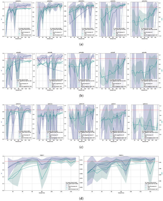
Figure 3.
Relationship between dataset size and model performance for different object detection models (YOLOv5 (a), YOLOv8 (b), YOLO11 (c), and RT-DETR (d)) trained and tested on ID datasets. On the same line, each subplot represents a different parameters size of the model, increasing from the left to the right. The x-axis represents the dataset size, while the left and right y-axis represents the and values, respectively. The solid lines represent the mean values, while the dashed lines indicate the logarithmic fit. The shaded area around the solid lines represents the confidence interval (standard deviation) of or . The red dashed horizontal line represents the benchmark value of 0.85. The combined legend in the lower right corner of each subplot shows the Goodness of Fit () for both and .
For the combinations of model-architecture/dataset-size that achieved the benchmark, the minimum dataset quality required to achieve the benchmark was evaluated, as shown in Figure 4. The minimum dataset quality was determined by identifying the quality percentage where both the empirical model prediction and the entire confidence interval of the performance metrics remained above the benchmark threshold.
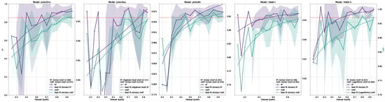
Figure 4.
Relationship between dataset quality and model performance for all object detection models that achieved the benchmark. The x-axis represents the dataset quality, while the left y-axis represents the values. The red dashed horizontal line represents the benchmark value of 0.85. The legend in the lower right corner of the subplot shows the Goodness of Fit () for .
Within YOLO models, YOLOv5n, YOLOv5s, and YOLOv8n achieve the benchmark value of 0.85 with 130, 130, and 110 samples, respectively, considering the dataset sizes where all three model performances were above 0.85 and the logarithmic model predicted over-benchmark values for that dataset size. RT-DETR L and RT-DETR X achieve the benchmark value of 0.85 with 60 and 100 samples, respectively, with the same assumptions as for the YOLO models. For these models, the was above 0.3, while for the models that did not reach the benchmark value the was always below this value. The seems to follow the same trend as the values. All the models show a clear trend of increasing and values as the dataset size increases, as expected. It is also clear that increasing the number of parameters and model complexity for mostly CNN-like models (YOLOs) leads to increasing need for dataset size. For the mostly transformer-like models (RT-DETRs), it is not that clear, also because of the low amount of model parameter sizes tested. The confidence interval reduction as a function of the dataset size indicates that variability in performance decreases significantly as dataset size increases for all models. Taking into account the dataset quality in the same way as done for the dataset size, both quality tests and quality models achieved the benchmark, with 85%, 90%, 85%, and 65% of the original dataset quality for YOLOv5n, YOLOv5s, YOLOv8n, and RT-DETR X, respectively. RT-DETR L did not achieve the benchmark for any dataset quality reduction tested. Overall, RT-DETR performed best in terms of both dataset size and quality. The best performance in terms of dataset size was achieved with RT-DETR trained on 60 images (see prediction examples in Figure 5), while the best performance in terms of dataset quality was achieved with RT-DETR trained on 100 images with a 35% reduction in quality (see Figure 6 for prediction examples).
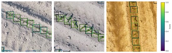
Figure 5.
Predictions from the RT-DETR L trained on 60 images. From the left hand side to the right hand side, the images show the 1, 2, and 3 ID test dataset tile examples. The predicted bounding boxes in the images are the ones before non-maximum suppression and threshold. Black bounding boxes are the ground truth annotations, while the bounding boxes in the viridis color scale are the model predictions.

Figure 6.
Predictions from the RT-DETR X trained on 100 images with a reduction in quality of 35%. From the left hand side to the right hand side, the images show the 1, 2, and 3 ID test dataset tile examples. The predicted bounding boxes in the images are the ones before non-maximum suppression and threshold. Black bounding boxes are the ground truth annotations, while the bounding boxes in the viridis color scale are the model predictions.
3.3. Few-Shot Object Detectors
The few-shot models were evaluated against the established benchmarks ( of 0.85 and of 0.39) using the metrics and ; however, none of the models reached these benchmarks.
The best result achieved by the CD-ViTO model was an of 3.9 with ViT-B backbone and 50 shots to build the prototypes, which is substantially worse than the benchmark value of 0.39 (10 times higher). This corresponds to a on counting of about 25% and a of about 0.5, as shown in Figure 7. It corresponds roughly to a miscounted plant over four as it is visible, looking to some predictions of this model in Figure 8. The models fitted on metrics show a reliable for all the metrics, indicating that the model performance is highly predictable by the number of shots. These also show that any CD-ViTO size model would not achieve the benchmark with any shot amount, even if the number of shots were increased beyond those tested.
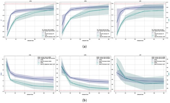
Figure 7.
The figure shows the relationship between shots and model performance for the CD-ViTO model trained and tested on ID datasets. The x-axis represents the number of shots. The solid lines represent the mean values, while the dashed lines indicate the shot amount/metric prediction model. The shaded area around the solid lines represents the confidence interval (standard deviation) of the metric. (a) The left and right y-axis represents the and values, respectively. The red dashed horizontal line represents the benchmark value of 0.85. The combined legend in the lower right corner of each subplot shows the Goodness of Fit () for both and . (b) The left and right y-axis represents the and values respectively. The red dashed horizontal line represents the benchmark value of 0.39. The combined legend in the upper right corner of each subplot shows the Goodness of Fit () for both and MAPE.

Figure 8.
The 50 shot CD-ViTO with ViT-B backbone predictions on the 1, 2, and 3 ID test dataset tile examples, respectively, from the left hand side to the right. The predicted bounding boxes in the images are the ones before non-maximum suppression and threshold. Black bounding boxes are the ground truth annotations, while the bounding boxes in the viridis color scale are the model predictions.
3.4. Zero-Shot Object Detectors
Figure 9 shows the relationship between the zero-shot model settings and model performance tested on ID testing datasets. Not all the model settings were able to predict the whole testing dataset. For example, the owlv2-base-patch16-finetuned model was not able to generate any prediction with any prompt for any image of the ID testing. A dataset size relationship with metrics could not be established because zero-shot models do not require fine-tuning training data. None of the zero-shot model settings reached the benchmark. This is particularly true for the values, which were always below 0, indicating poor predictive performance. The values ranged from approximately 5 to 25, significantly higher than those observed in the many-shot and few-shot models. Additionally, values were also considerably elevated, ranging from around 40 to 140. Furthermore, the values were lower than those of the many and few-shot models for all model settings, except for the owlv2-large-patch14-finetuned model, for which very few images were successfully predicted with an comparable to that of the best few-shot model (50-shots ViT-B backbone). Some rare cases of good predictions were even more accurate than the few-shot best performance, as shown in Figure 10.

Figure 9.
The figure shows the relationship between the OWLv2 model size, used prompt, and model performance. The x-axis represents the model settings and the model size. Colors represent the different prompts used. The four subplots show the (upper left corner), (upper right corner), (lower left corner), and MAPE (lower right corner) values. The red dashed horizontal line in the and the subplots represents, respectively, the benchmarks of 0.85 and 0.39.

Figure 10.
The best predictions with the OWLv2 model. The ID_1, ID_2, and ID_3 datasets, respectively, from the left hand side to the right. Prediction with owlv2-base-patch16-ensemble model of the ID_1 dataset, and with owlv2-base-patch16 model on the other two datasets. All the predictions are made with the prompt “seedling”. The predicted bounding boxes in the images are the ones before non-maximum suppression and threshold. Black bounding boxes are the ground truth annotations, while the bounding boxes in the viridis color scale are the model predictions.
4. Discussion
4.1. Dataset Source Impact on Object Detection Performance
Our experiments clearly demonstrate the critical importance of dataset source for successful arable crop seedling detection. None of the tested models, regardless of architecture or parameter amount, achieved the benchmark value of 0.85 when trained on Out-of-Distribution (OOD) datasets. Several inherent biases in our datasets likely influenced model performance. This aligns with previous findings by David et al. [16] and Andvaag et al. [47], who similarly reported significantly lower performance when using training samples from sources different from the inference dataset.
The domain gap challenge is particularly pronounced in agricultural applications, where environmental conditions, lighting, camera parameters, and plant growth stages vary substantially across datasets. The failure of OOD training highlights that visual features learned from one orthomosaic do not generalize well to others without significant adaptation. As the Goodness-of-Fit () of the models explicating the relationship between dataset size and performance was always below 0.2, one can argue that the interval of dataset size tested was too narrow to achieve a good fit or that other variables play an important role in determining model performance. Both cases are likely to be true, but also the maximum OOD dataset size that was tested (1168) was really small in respect to other studies that use training datasets of tens of thousand of images to achieve such benchmarks [33]. This further highlights the importance of collecting in-domain training data, as the minimum OOD dataset size and quality to train an object detector to count arable crops seedling that generalizes to all the real-world cases is difficult to establish with a limited dataset.
Despite the poor performance of OOD dataset-trained models, some of them showed a low value of less than 20%, not enough to consider the models for direct inferencing but rather as an annotation tool for the ID dataset.
4.2. Many-Shot Object Detection: Architecture and Dataset Requirements
Our results reveal important relationships between model architecture, count metrics, and minimum dataset requirements, consistent with findings from other agricultural computer vision studies. Within YOLO-family models, we observed that the lightweight YOLOv5n, YOLOv5s, and YOLOv8n achieved the benchmark with 130, 130, and 110 samples, respectively, well below the reported minimum by supposed few-shot studies with the same aim [43]. As already well-known from general computer vision literature [48,52], increasing model complexity in CNN-based architectures corresponded to increased dataset size requirements.
Conversely, for transformer-mixed models like RT-DETR, we observed better performances with lower training dataset sizes, with RT-DETR L achieving the benchmark with only 60 samples while the larger RT-DETR X required 100 samples. This superior performance of transformer-based models corroborates recent findings [34,35], who demonstrated that attention mechanisms can achieve better performance with limited training data in agricultural contexts. The empirical models of dataset size versus performance showed comparable between RT-DETR and YOLO-family models, except for YOLOv5n, which showed a particularly high . This suggests that transformer-based models have the same predictability to reach the benchmark with the reported dataset size as the CNN-based models, except for YOLOv5n, which has a higher predictability to reach the benchmark given the same dataset size.
Overall, transformer-based models may require fewer samples to achieve the same performance as CNN-based models, potentially due to their ability to capture long-range dependencies and contextual information more effectively, as noted in a comprehensive review [32] and demonstrated in agricultural applications [33]. A visible side-effect of the adoption of transformer-mixed models is the higher computational cost of the training phase in terms of time and memory, which could be a limitation for some applications, consistent with computational trade-offs reported in [28] but not studied here.
This creates a practical tradeoff for practitioners: whether to use a simpler CNN-based model like YOLOv5n and invest in collecting more annotated images (approximately 130), or to allocate more computational resources for a transformer-mixed model like RT-DETR L that can achieve comparable performance with roughly half the amount of labeled data (approximately 60 images). Similar trade-offs have been documented in agricultural deployment scenarios by [21] for early-season crop monitoring and [33] in their comprehensive review of agricultural object detection.
The predictability of model performance based on dataset size (as evidenced by values exceeding 0.3 for successful models) provides practical guidance for practitioners. Our findings on dataset size scaling relationships (logarithmic patterns with GoF > 0.3) align with broader machine learning scaling laws established by [48,50], while the agricultural-specific implications mirror domain adaptation challenges documented in [16,47]. The relationship between dataset size and performance (modeled using logarithmic, arctangent, or algebraic root functions, depending on best fit) suggests diminishing returns beyond certain thresholds, consistent with theoretical frameworks proposed by [51], which can help inform efficient resource allocation for annotation efforts in precision agriculture applications.
4.3. Dataset Quality Trade-Offs
Our investigation into minimum dataset quality requirements revealed that models can tolerate some reduction in annotation quality while still maintaining benchmark performance achieved with the same training dataset size. YOLOv5n, YOLOv5s, and YOLOv8n achieved the benchmark with 85%, 90%, and 85% of the original dataset quality, while RT-DETR X required only 65%. Notably, RT-DETR L failed to maintain benchmark performance with any reduction in annotation quality, suggesting different sensitivity to annotation errors, consistent with findings on annotation quality effects [49].
This difference in quality tolerance between RT-DETR L and RT-DETR X can be explained by considering their respective minimum dataset sizes. RT-DETR L was tested with quality reductions on its minimum benchmark-achieving dataset size of just 60 samples, while RT-DETR X was tested with 100 samples. With fewer training examples, RT-DETR L becomes more sensitive to the quality of each individual annotation, as each annotation represents a larger proportion of the total learning signal. In contrast, RT-DETR X, with its larger training dataset, can better compensate for quality reductions by leveraging redundancy across more examples, aligning with general principles of dataset robustness [48].
These findings provide valuable insights for practical applications, as they suggest that, in some cases, it may be more efficient to collect a larger quantity of moderate-quality annotations rather than focusing on perfect annotations for a smaller dataset. This also indicates potential for semi-automated annotation workflows, where machine assistance in annotation (which may introduce some errors) could be acceptable for many applications, supporting approaches documented in agricultural computer vision literature [33].
4.4. Few-Shot and Zero-Shot Approaches: Current Limitations
Despite recent advances in few-shot and zero-shot learning, our experiments reveal significant limitations in these approaches for precise maize seedling detection. The best CD-ViTO few-shot model achieved an of 3.9 with 50 shots (using ViT-B backbone), substantially below the benchmark requirement of 0.39. Similarly, zero-shot models like OWLv2 performed poorly, regardless of prompt engineering efforts.
These results contrast with the promising performance reported for few-shot and zero-shot methods in general object detection benchmarks [41,74]. Several factors may explain this gap: First, the domain-specific nature of aerial maize seedling imagery, where subtle textural differences and high intra-class variability are prevalent, severely challenges models pre-trained on general object detection datasets. As illustrated in the few-shot experiments (Figure 7), increasing the number of shots leads to nonlinear improvements in metrics such as R2 and (following an arctan-like trend), yet the error metric () remain significantly above the benchmark. This saturation effect suggests that, even with more than usual maximum tested prototypes (50 instead of 30), the models struggle to capture the fine-grained visual cues necessary for precise seedling detection. Moreover, the zero-shot results (Figure 9) reveal a pronounced sensitivity to prompt phrasing, with all variants, including ensemble and fine-tuned versions of OWLv2, consistently failing to approach acceptable error rates. These observations imply that both the inherent complexity of the task and the limitations of current few-shot and zero-shot frameworks necessitate more domain-specific strategies, as suggested by recent work on agricultural computer vision challenges [14]. Addressing these challenges through domain-specific adaptations could help narrow the performance gap, potentially making few-shot and zero-shot methods more competitive for arable crop seedling detection. Interestingly, the few-shot and the zero-shot models were able to detect all the seedlings without false positives in few cases. It would be interesting to investigate the possible ways to retain these images and use them to populate the training dataset for a many-shot model.
4.5. Handcrafted Methods in the Deep Learning Era
Despite the focus on deep learning approaches, our Handcrafted (HC) object detector demonstrated strong performance on the testing datasets ( from 0.87 to 0.95). However, a significant limitation was the small proportion of tiles (1.8% to 7.8%) for which it could provide reliable annotations. This illustrates the classic trade-off of rule-based systems: high precision in constrained scenarios but limited generalizability, consistent with findings from other agricultural applications using handcrafted methods [22,23].
These findings suggest that HC methods may still have value in a hybrid approach, where they provide high-quality annotations on a subset of data, which can then be used to bootstrap deep learning models. Such an approach could be particularly valuable for specialized agricultural applications where annotation resources are limited, aligning with hybrid approaches documented in crop monitoring studies [21].
This approach is highly adopted in industry, where the HC method is used to annotate the training dataset and the deep learning model is used to predict the real-world cases, but it introduces a possible bias in the training dataset that could be a limitation for the model generalization. The main problem is that the HC1 method relies on color thresholding that filters the objects based on the color of the objects. That could be not the best way to annotate the training dataset for a deep learning model that could learn more complex features of the objects, but also the ones selected by the HC1 method.
4.6. Implications for Practical Applications
Our study has several practical implications for developing arable crop seedling detection systems. First, collecting in-domain training data is non-negotiable for achieving benchmark performance. Finding a way to automatically obtain the training dataset from the same distribution as the intended inference target is a key step in developing a robust object detector for arable crop seedling detection.
The logarithmic relationship between dataset size and performance suggests that initial annotation efforts should focus on reaching the minimum viable dataset size (60–130 images depending on architecture), after which additional annotations yield diminishing returns. This finding helps organizations optimize resource allocation for annotation efforts.
Our results also demonstrate that some reduction in annotation quality is acceptable, with models maintaining benchmark performance with 65–90% of the original quality. This suggests that semi-automated annotation workflows could be efficiently implemented for agricultural applications, potentially reducing the time and cost associated with manual annotation.
Current few-shot and zero-shot methods, while promising, are not yet viable replacements for traditional object detection approaches in seedling detection or counting tasks. However, they might still serve auxiliary roles in the annotation pipeline.
Hybrid approaches combining handcrafted methods with deep learning models could provide a practical solution for achieving benchmark performance. We observed that OOD many-shot, few-shot, and zero-shot models are occasionally able to produce annotations with sufficient quality for training ID many-shot models. A promising direction for future work would be to develop methods for automatically identifying and leveraging these high-quality annotations. Specifically, the HC2 component of our handcrafted approach could potentially be used to filter and validate annotations produced by these models, overcoming the color-thresholding bias introduced by HC1 while maintaining the agronomic knowledge encoded in HC2’s row-pattern validation.
4.7. Future Work
In this study, we focused on the minimum dataset requirements for fine-tuning pre-trained models for the downstream task of counting arable crop seedlings through object detection. We did not explore the potential benefits of using domain-specific backbones. Future work could investigate whether or not dataset size requirements could be further reduced by using backbones pre-trained on agricultural imagery, particularly aerial orthomosaics of crop fields. Such domain-specific pre-training might allow models to learn more relevant features for crop detection tasks, potentially reducing the amount of in-domain data needed for fine-tuning.
5. Conclusions
This study demonstrates that successful maize seedling detection requires in-domain training data, with out-of-distribution training requiring unreasonable dataset size to achieve benchmark performance across all tested models. We established minimum dataset requirements for several architectures, finding that lightweight YOLO models achieve benchmark performance with 110–130 samples, while certain transformer-mixed models like RT-DETR require as few as 60 samples. Models showed varying tolerance for reduced annotation quality, with some maintaining performance with only 65–90% of original annotation quality.
Despite advances in machine learning, neither few-shot nor zero-shot approaches currently meet precision requirements for arable crop seedling detection. Our handcrafted algorithm achieved excellent performance within its constraints, suggesting potential value in hybrid approaches combining rule-based methods with deep learning. These findings provide practical guidance for developing maize seedling detection systems, and possible ways to overcome the limitations of the current deep learning models for this application.
Author Contributions
Conceptualization, S.B. and E.B.-M.; methodology, S.B. and E.B.-M.; software, S.B.; validation, S.B.; formal analysis, S.B.; investigation, S.B.; resources, S.B. and E.B.-M.; data curation, S.B.; writing—original draft preparation, S.B.; writing—review and editing, E.B.-M.; visualization, S.B.; supervision, E.B.-M.; project administration, E.B.-M.; funding acquisition, S.B. and E.B.-M. All authors have read and agreed to the published version of the manuscript.
Funding
This research was conducted as part of a PhD program supported by SAGEA centro di saggio s.r.l.
Data Availability Statement
The code for the handcrafted methods used in this study is available at https://gist.github.com/SamueleBumbaca/4a227bbe7b78d6be3424899c16c60bb4 (accessed on 20 June 2025). The datasets created during this study (ID datasets) are available at the Zenodo repository https://doi.org/10.5281/zenodo.15235602 (accessed on 20 June 2025). The other datasets used are available from their cited sources.
Conflicts of Interest
The authors declare no conflicts of interest. The funders had no role in the design of the study; in the collection, analyses, or interpretation of data; in the writing of the manuscript; or in the decision to publish the results.
Abbreviations
The following abbreviations are used in this manuscript:
| Coefficient of determination | |
| Root Mean Squared Error | |
| Mean Absolute Percentage Error | |
| Mean Average Precision | |
| HC | Handcrafted |
| ID | In-Distribution |
| OOD | Out-of-Distribution |
| CNN | Convolutional Neural Network |
| ViT | Vision Transformer |
| YOLO | You Only Look Once |
| RT-DETR | Real-Time Detection Transformer |
| GoF | Goodness of Fit |
Appendix A
Appendix A.1
| Algorithm A1 H1 |
|
| Algorithm A2 H2 |
|
Appendix A.2
The following are the list of prompts used for the zero-shot models:
- “maize”
- “seedling”
- “plant”
- “aerial view of maize seedlings”
- “corn seedlings in rows”
- “young maize plants from above”
- “crop rows with corn seedlings”
- “maize seedlings with regular spacing”
- “top-down view of corn plants”
- “agricultural field with maize seedlings”
- “orthomosaic of corn plants in rows”
References
- Blandino, M.; Testa, G.; Quaglini, L.; Reyneri, A. Effetto Della Densità Colturale e Dell’Applicazione di Fungicidi Sulla Produzione e la Qualità del Mais da Granella e da Trinciato; ITA: Rome, Italy, 2016. [Google Scholar]
- Lu, D.; Ye, J.; Wang, Y.; Yu, Z. Plant Detection and Counting: Enhancing Precision Agriculture in UAV and General Scenes. IEEE Access 2023, 11, 116196–116205. [Google Scholar] [CrossRef]
- Saatkamp, A.; Cochrane, A.; Commander, L.; Guja, L.; Jimenez-Alfaro, B.; Larson, J.; Nicotra, A.; Poschlod, P.; Silveira, F.A.O.; Cross, A.; et al. A research agenda for seed-trait functional ecology. New Phytol. 2019, 221, 1764–1775. [Google Scholar] [CrossRef] [PubMed]
- De Petris, S.; Sarvia, F.; Gullino, M.; Tarantino, E.; Borgogno-Mondino, E. Sentinel-1 Polarimetry to Map Apple Orchard Damage after a Storm. Remote Sens. 2021, 13, 1030. [Google Scholar] [CrossRef]
- PP 1/333 (1) Adoption of Digital Technology for Data Generation for the Efficacy Evaluation of Plant Protection Products. EPPO Bull. 2025, 55, 14–19. [CrossRef]
- Zou, H.; Lu, H.; Li, Y.; Liu, L.; Cao, Z. Maize Tassels Detection: A Benchmark of the State of the Art. Plant Methods 2020, 16, 108. [Google Scholar] [CrossRef]
- Lin, T.Y.; Maire, M.; Belongie, S.; Bourdev, L.; Girshick, R.; Hays, J.; Perona, P.; Ramanan, D.; Zitnick, C.L.; Dollár, P. Microsoft COCO: Common Objects in Context. arXiv 2015, arXiv:1405.0312. [Google Scholar]
- Kraus, K. Photogrammetry: Geometry from Images and Laser Scans; De Gruyter: Berlin, Germany, 2011. [Google Scholar] [CrossRef]
- Pugh, N.A.; Thorp, K.R.; Gonzalez, E.M.; Elshikha, D.E.M.; Pauli, D. Comparison of image georeferencing strategies for agricultural applications of small unoccupied aircraft systems. Plant Phenome J. 2021, 4, e20026. [Google Scholar] [CrossRef]
- Dhonju, H.K.; Walsh, K.B.; Bhattarai, T. Web Mapping for Farm Management Information Systems: A Review and Australian Orchard Case Study. Agronomy 2023, 13, 2563. [Google Scholar] [CrossRef]
- Habib, A.; Han, Y.; Xiong, W.; He, F.; Zhang, Z.; Crawford, M. Automated Ortho-Rectification of UAV-Based Hyperspectral Data over an Agricultural Field Using Frame RGB Imagery. Remote Sens. 2016, 8, 796. [Google Scholar] [CrossRef]
- De Petris, S.; Sarvia, F.; Borgogno-Mondino, E. RPAS-based photogrammetry to support tree stability assessment: Longing for precision arboriculture. Urban For. Urban Green. 2020, 55, 126862. [Google Scholar] [CrossRef]
- Zhang, S.; Barrett, H.A.; Baros, S.V.; Neville, P.R.H.; Talasila, S.; Sinclair, L.L. Georeferencing Accuracy Assessment of Historical Aerial Photos Using a Custom-Built Online Georeferencing Tool. ISPRS Int. J. Geo-Inf. 2022, 11, 582. [Google Scholar] [CrossRef]
- Farjon, G.; Huijun, L.; Edan, Y. Deep-learning-based counting methods, datasets, and applications in agriculture: A review. Precis. Agric. 2023, 24, 1683–1711. [Google Scholar] [CrossRef]
- Meier, U.; Bleiholder, H.; Buhr, L.; Feller, C.; Hack, H.; Heß, M.; Lancashire, P.D.; Schnock, U.; Stauß, R.; van den Boom, T.; et al. The BBCH System to Coding the Phenological Growth Stages of Plants-History and Publications. J. Für Kult. 2009, 61, 41–52. [Google Scholar] [CrossRef]
- David, E.; Daubige, G.; Joudelat, F.; Burger, P.; Comar, A.; de Solan, B.; Baret, F. Plant Detection and Counting from High-Resolution RGB Images Acquired from UAVs: Comparison between Deep-Learning and Handcrafted Methods with Application to Maize, Sugar Beet, and Sunflower. bioRxiv 2021. [Google Scholar] [CrossRef]
- Liu, W.; Zhou, J.; Wang, B.; Costa, M.; Kaeppler, S.M.; Zhang, Z. IntegrateNet: A Deep Learning Network for Maize Stand Counting From UAV Imagery by Integrating Density and Local Count Maps. IEEE Geosci. Remote Sens. Lett. 2022, 19, 6512605. [Google Scholar] [CrossRef]
- Maize_seeding Dataset > Overview. Available online: https://universe.roboflow.com/objectdetection-hytat/maize_seeding (accessed on 20 June 2025).
- Maize-Seedling-Detection Dataset > Overview. Available online: https://universe.roboflow.com/fyxdds-icloud-com/maize-seedling-detection (accessed on 20 June 2025).
- FAO. Agricultural Production Statistics 2010–2023; Volume Analytical Briefs; FAOSTAT: Rome, Italy, 2024. [Google Scholar]
- Torres-Sánchez, J.; Mesas-Carrascosa, F.J.; Jiménez-Brenes, F.M.; de Castro, A.I.; López-Granados, F. Early Detection of Broad-Leaved and Grass Weeds in Wide Row Crops Using Artificial Neural Networks and UAV Imagery. Agronomy 2021, 11, 749. [Google Scholar] [CrossRef]
- Zhang, Z.; Cao, R.; Peng, C.; Liu, R.; Sun, Y.; Zhang, M.; Li, H. Cut-edge detection method for rice harvesting based on machine vision. Agronomy 2020, 10, 590. [Google Scholar] [CrossRef]
- García-Martínez, H.; Flores-Magdaleno, H.; Khalil-Gardezi, A.; Ascencio-Hernández, R.; Tijerina-Chávez, L.; Vázquez-Peña, M.A.; Mancilla-Villa, O.R. Digital Count of Corn Plants Using Images Taken by Unmanned Aerial Vehicles and Cross Correlation of Templates. Agronomy 2020, 10, 469. [Google Scholar] [CrossRef]
- LeCun, Y.; Bengio, Y.; Hinton, G. Deep Learning. Nature 2015, 521, 436–444. [Google Scholar] [CrossRef]
- Faster R-CNN: Towards Real-Time Object Detection with Region Proposal Networks|IEEE Journals & Magazine|IEEE Xplore. Available online: https://ieeexplore-ieee-org.bibliopass.unito.it/document/7485869 (accessed on 20 June 2025).
- You Only Look Once: Unified, Real-Time Object Detection|IEEE Conference Publication|IEEE Xplore. Available online: https://ieeexplore-ieee-org.bibliopass.unito.it/document/7780460 (accessed on 20 June 2025).
- Vaswani, A.; Shazeer, N.; Parmar, N.; Uszkoreit, J.; Jones, L.; Gomez, A.N.; Kaiser, Ł.; Polosukhin, I. Attention Is All You Need. In Proceedings of the 31st International Conference on Neural Information Processing Systems, Long Beach, CA, USA, 4–9 December 2017; NIPS’17. pp. 6000–6010. [Google Scholar]
- Carion, N.; Massa, F.; Synnaeve, G.; Usunier, N.; Kirillov, A.; Zagoruyko, S. End-to-End Object Detection with Transformers. arXiv 2020, arXiv:2005.12872. [Google Scholar]
- Dosovitskiy, A.; Beyer, L.; Kolesnikov, A.; Weissenborn, D.; Zhai, X.; Unterthiner, T.; Dehghani, M.; Minderer, M.; Heigold, G.; Gelly, S.; et al. An Image Is Worth 16x16 Words: Transformers for Image Recognition at Scale. arXiv 2021, arXiv:2010.11929. [Google Scholar]
- Russakovsky, O.; Deng, J.; Su, H.; Krause, J.; Satheesh, S.; Ma, S.; Fei-Fei, L. ImageNet Large Scale Visual Recognition Challenge. Int. J. Comput. Vis. 2014, 115, 211–252. [Google Scholar] [CrossRef]
- Zong, Z.; Song, G.; Liu, Y. DETRs with Collaborative Hybrid Assignments Training. In Proceedings of the 2023 IEEE/CVF International Conference on Computer Vision (ICCV), Paris, France, 1–6 October 2023; pp. 6725–6735. [Google Scholar] [CrossRef]
- Khan, A.; Rauf, Z.; Sohail, A.; Khan, A.R.; Asif, H.; Asif, A.; Farooq, U. A Survey of the Vision Transformers and Their CNN-transformer Based Variants. Artif. Intell. Rev. 2023, 56, 2917–2970. [Google Scholar] [CrossRef]
- Badgujar, C.M.; Poulose, A.; Gan, H. Agricultural Object Detection with You Only Look Once (YOLO) Algorithm: A Bibliometric and Systematic Literature Review. Comput. Electron. Agric. 2024, 223, 109090. [Google Scholar] [CrossRef]
- Rekavandi, A.M.; Rashidi, S.; Boussaid, F.; Hoefs, S.; Akbas, E.; Bennamoun, M. Transformers in Small Object Detection: A Benchmark and Survey of State-of-the-Art. arXiv 2023, arXiv:2309.04902. [Google Scholar]
- Li, Y.; Miao, N.; Ma, L.; Shuang, F.; Huang, X. Transformer for Object Detection: Review and Benchmark. Eng. Appl. Artif. Intell. 2023, 126, 107021. [Google Scholar] [CrossRef]
- Zhao, Y.; Lv, W.; Xu, S.; Wei, J.; Wang, G.; Dang, Q.; Liu, Y.; Chen, J. DETRs Beat YOLOs on Real-time Object Detection. arXiv 2024, arXiv:2304.08069. [Google Scholar]
- Khanam, R.; Hussain, M. YOLOv11: An Overview of the Key Architectural Enhancements. arXiv 2024, arXiv:2410.17725. [Google Scholar]
- Li, Z.; Zhou, F.; Chen, F.; Li, H. Meta-SGD: Learning to Learn Quickly for Few-Shot Learning. arXiv 2017, arXiv:1707.09835. [Google Scholar]
- Bansal, A.; Sikka, K.; Sharma, G.; Chellappa, R.; Divakaran, A. Zero-Shot Object Detection. In Proceedings of the European Conference on Computer Vision (ECCV), Munich, Germany, 8–14 September 2018; pp. 384–400. [Google Scholar]
- Kang, B.; Liu, Z.; Wang, X.; Yu, F.; Feng, J.; Darrell, T. Few-Shot Object Detection via Feature Reweighting. arXiv 2019, arXiv:1812.01866. [Google Scholar]
- Minderer, M.; Gritsenko, A.; Houlsby, N. Scaling Open-Vocabulary Object Detection. Adv. Neural Inf. Process. Syst. 2023, 36, 72983–73007. [Google Scholar]
- Liu, S.; Zeng, Z.; Ren, T.; Li, F.; Zhang, H.; Yang, J.; Jiang, Q.; Li, C.; Yang, J.; Su, H.; et al. Grounding DINO: Marrying DINO with Grounded Pre-training for Open-Set Object Detection. In Proceedings of the Computer Vision—ECCV 2024, Milan, Italy, 29 September–4 October 2024; Leonardis, A., Ricci, E., Roth, S., Russakovsky, O., Sattler, T., Varol, G., Eds.; Springer: Cham, Switzerland, 2025; pp. 38–55. [Google Scholar] [CrossRef]
- Karami, A.; Crawford, M.; Delp, E.J. Automatic Plant Counting and Location Based on a Few-Shot Learning Technique. IEEE J. Sel. Top. Appl. Earth Obs. Remote Sens. 2020, 13, 5872–5886. [Google Scholar] [CrossRef]
- Wang, D.; Parthasarathy, R.; Pan, X. Advancing Image Recognition: Towards Lightweight Few-shot Learning Model for Maize Seedling Detection. In Proceedings of the 2024 International Conference on Smart City and Information System, Kuala Lumpur, Malaysia, 17–19 May 2024; pp. 635–639. [Google Scholar] [CrossRef]
- Barreto, A.; Lottes, P.; Ispizua Yamati, F.R.; Baumgarten, S.; Wolf, N.A.; Stachniss, C.; Mahlein, A.K.; Paulus, S. Automatic UAV-based Counting of Seedlings in Sugar-Beet Field and Extension to Maize and Strawberry. Comput. Electron. Agric. 2021, 191, 106493. [Google Scholar] [CrossRef]
- Kitano, B.T.; Mendes, C.C.T.; Geus, A.R.; Oliveira, H.C.; Souza, J.R. Corn Plant Counting Using Deep Learning and UAV Images. IEEE Geosci. Remote Sens. Lett. 2019, 16, 1–5. [Google Scholar] [CrossRef]
- Andvaag, E.; Krys, K.; Shirtliffe, S.J.; Stavness, I. Counting Canola: Toward Generalizable Aerial Plant Detection Models. Plant Phenomics 2024, 6, 0268. [Google Scholar] [CrossRef]
- Sun, C.; Shrivastava, A.; Singh, S.; Gupta, A. Revisiting Unreasonable Effectiveness of Data in Deep Learning Era. arXiv 2017, arXiv:1707.02968. [Google Scholar]
- Alhazmi, K.; Alsumari, W.; Seppo, I.; Podkuiko, L.; Simon, M. Effects of Annotation Quality on Model Performance. In Proceedings of the 2021 International Conference on Artificial Intelligence in Information and Communication (ICAIIC), Jeju Island, Republic of Korea, 13–16 April 2021; pp. 063–067. [Google Scholar] [CrossRef]
- Hestness, J.; Narang, S.; Ardalani, N.; Diamos, G.; Jun, H.; Kianinejad, H.; Patwary, M.M.A.; Yang, Y.; Zhou, Y. Deep Learning Scaling Is Predictable, Empirically. arXiv 2017, arXiv:1712.00409. [Google Scholar]
- Mahmood, R.; Lucas, J.; Acuna, D.; Li, D.; Philion, J.; Alvarez, J.M.; Yu, Z.; Fidler, S.; Law, M.T. How Much More Data Do I Need? Estimating Requirements for Downstream Tasks. In Proceedings of the 2022 IEEE/CVF Conference on Computer Vision and Pattern Recognition (CVPR), New Orleans, LA, USA, 18–24 June 2022; pp. 275–284. [Google Scholar] [CrossRef]
- Nguyen, N.D.; Do, T.; Ngo, T.D.; Le, D.D.; Valenti, C.F. An Evaluation of Deep Learning Methods for Small Object Detection. JECE 2020, 2020, 8856387. [Google Scholar] [CrossRef]
- Du, X.; Lin, T.Y.; Jin, P.; Ghiasi, G.; Tan, M.; Cui, Y.; Le, Q.V.; Song, X. SpineNet: Learning Scale-Permuted Backbone for Recognition and Localization. In Proceedings of the IEEE/CVF Conference on Computer Vision and Pattern Recognition, Seattle, WA, USA, 13–19 June 2020; pp. 11592–11601. [Google Scholar]
- Shorten, C.; Khoshgoftaar, T.M. A Survey on Image Data Augmentation for Deep Learning. J. Big Data 2019, 6, 60. [Google Scholar] [CrossRef]
- Liu, S.; Yin, D.; Feng, H.; Li, Z.; Xu, X.; Shi, L.; Jin, X. Estimating Maize Seedling Number with UAV RGB Images and Advanced Image Processing Methods. Precis. Agric. 2022, 23, 1604–1632. [Google Scholar] [CrossRef]
- Velumani, K.; Lopez-Lozano, R.; Madec, S.; Guo, W.; Gillet, J.; Comar, A.; Baret, F. Estimates of Maize Plant Density from UAV RGB Images Using Faster-RCNN Detection Model: Impact of the Spatial Resolution. Plant Phenomics 2021, 2021, 9824843. [Google Scholar] [CrossRef]
- Bumbaca, S. The Original Dataset for the Paper “On the minimum dataset requirements for fine-tuning an object detector for arable crop plant counting: A case study on maize seedlings”. Zenodo 2025. [Google Scholar] [CrossRef]
- Krizhevsky, A.; Sutskever, I.; Hinton, G.E. ImageNet Classification with Deep Convolutional Neural Networks. In Advances in Neural Information Processing Systems; Curran Associates, Inc.: Nice, France, 2012; Volume 25. [Google Scholar]
- Fischler, M.A.; Bolles, R.C. Random Sample Consensus: A Paradigm for Model Fitting with Applications to Image Analysis and Automated Cartography. In Readings in Computer Vision; Fischler, M.A., Firschein, O., Eds.; Morgan Kaufmann: San Francisco, CA, USA, 1987; pp. 726–740. [Google Scholar] [CrossRef]
- Terven, J.; Córdova-Esparza, D.M.; Romero-González, J.A. A Comprehensive Review of YOLO Architectures in Computer Vision: From YOLOv1 to YOLOv8 and YOLO-NAS. Mach. Learn. Knowl. Extr. 2023, 5, 1680–1716. [Google Scholar] [CrossRef]
- Jocher, G.; Qiu, J.; Chaurasia, A. GitHub Ultralytics YOLO. 2023. Available online: https://github.com/ultralytics/ultralytics (accessed on 16 April 2025).
- Oquab, M.; Darcet, T.; Moutakanni, T.; Vo, H.; Szafraniec, M.; Khalidov, V.; Fernandez, P.; Haziza, D.; Massa, F.; El-Nouby, A.; et al. DINOv2: Learning Robust Visual Features without Supervision. arXiv 2024, arXiv:2304.07193. [Google Scholar]
- Fu, Y.; Wang, Y.; Pan, Y.; Huai, L.; Qiu, X.; Shangguan, Z.; Liu, T.; Fu, Y.; Gool, L.V.; Jiang, X. Cross-Domain Few-Shot Object Detection via Enhanced Open-Set Object Detector. arXiv 2024, arXiv:2402.03094. [Google Scholar]
- Wolf, T.; Debut, L.; Sanh, V.; Chaumond, J.; Delangue, C.; Moi, A.; Cistac, P.; Rault, T.; Louf, R.; Funtowicz, M.; et al. Transformers: State-of-the-Art Natural Language Processing. In Proceedings of the 2020 Conference on Empirical Methods in Natural Language Processing: System Demonstrations, Online, 16–20 November 2020; pp. 38–45. [Google Scholar]
- Zhu, H.; Qin, S.; Su, M.; Lin, C.; Li, A.; Gao, J. Harnessing Large Vision and Language Models in Agriculture: A Review. arXiv 2024, arXiv:2407.19679. [Google Scholar]
- Zhou, Y.; Yan, H.; Ding, K.; Cai, T.; Zhang, Y. Few-Shot Image Classification of Crop Diseases Based on Vision–Language Models. Sensors 2024, 24, 6109. [Google Scholar] [CrossRef]
- Chen, H.; Huang, W.; Ni, Y.; Yun, S.; Liu, Y.; Wen, F.; Velasquez, A.; Latapie, H.; Imani, M. TaskCLIP: Extend Large Vision-Language Model for Task Oriented Object Detection. arXiv 2024, arXiv:2403.08108. [Google Scholar]
- Chicco, D.; Warrens, M.J.; Jurman, G. The coefficient of determination R-squared is more informative than SMAPE, MAE, MAPE, MSE and RMSE in regression analysis evaluation. PeerJ Comput. Sci. 2021, 7, e623. [Google Scholar] [CrossRef]
- Draper, N.R.; Smith, H. Applied Regression Analysis; John Wiley & Sons: Hoboken, NJ, USA, 1998; Volume 326. [Google Scholar]
- Armstrong, J.; Collopy, F. Error measures for generalizing about forecasting methods: Empirical comparisons. Int. J. Forecast. 1992, 8, 69–80. [Google Scholar] [CrossRef]
- Everingham, M.; Van Gool, L.; Williams, C.K.I.; Winn, J.; Zisserman, A. The Pascal Visual Object Classes (VOC) Challenge. Int. J. Comput. Vis. 2010, 88, 303–338. [Google Scholar] [CrossRef]
- Vianna, L.S.; Gonçalves, A.L.; Souza, J.A. Analysis of learning curves in predictive modeling using exponential curve fitting with an asymptotic approach. PLoS ONE 2024, 19, e0299811. [Google Scholar] [CrossRef]
- Akyon, F.C.; Altinuc, S.O.; Temizel, A. Slicing Aided Hyper Inference and Fine-tuning for Small Object Detection. In Proceedings of the 2022 IEEE International Conference on Image Processing (ICIP), Bordeaux, France, 16–19 October 2022; pp. 966–970. [Google Scholar] [CrossRef]
- Xu, G.; Hao, Z.; Luo, Y.; Hu, H.; An, J.; Mao, S. DeViT: Decomposing Vision Transformers for Collaborative Inference in Edge Devices. arXiv 2023, arXiv:2309.05015. [Google Scholar] [CrossRef]
- Wu, K.; Otoo, E.; Shoshani, A. Optimizing Connected Component Labeling Algorithms. In Proceedings of the Medical Imaging 2005: Image Processing, San Diego, CA, USA, 12–17 February 2005. [Google Scholar]
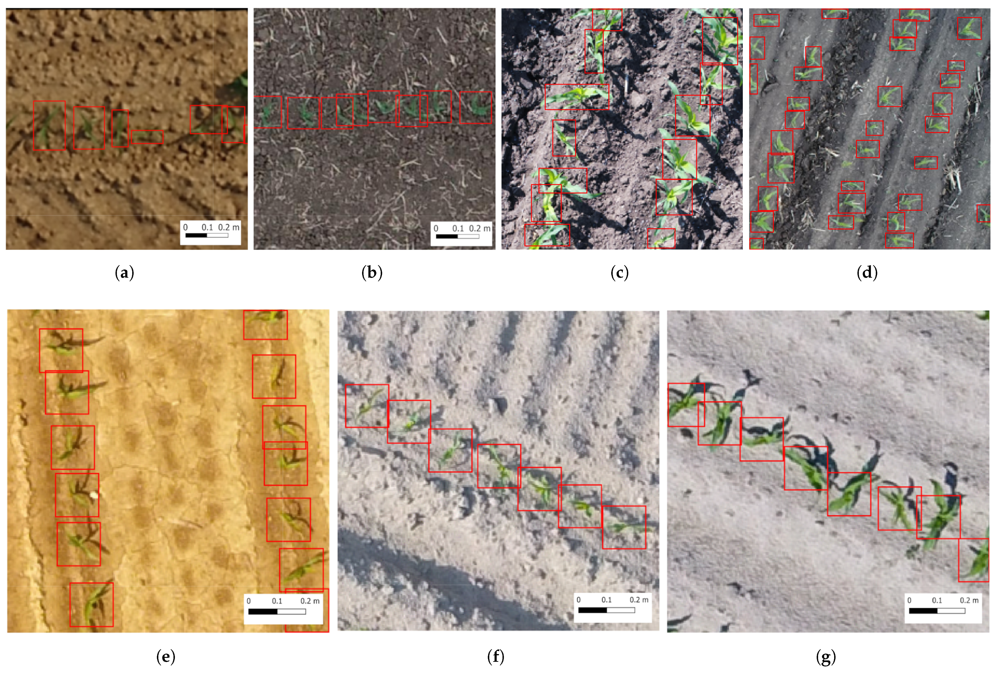
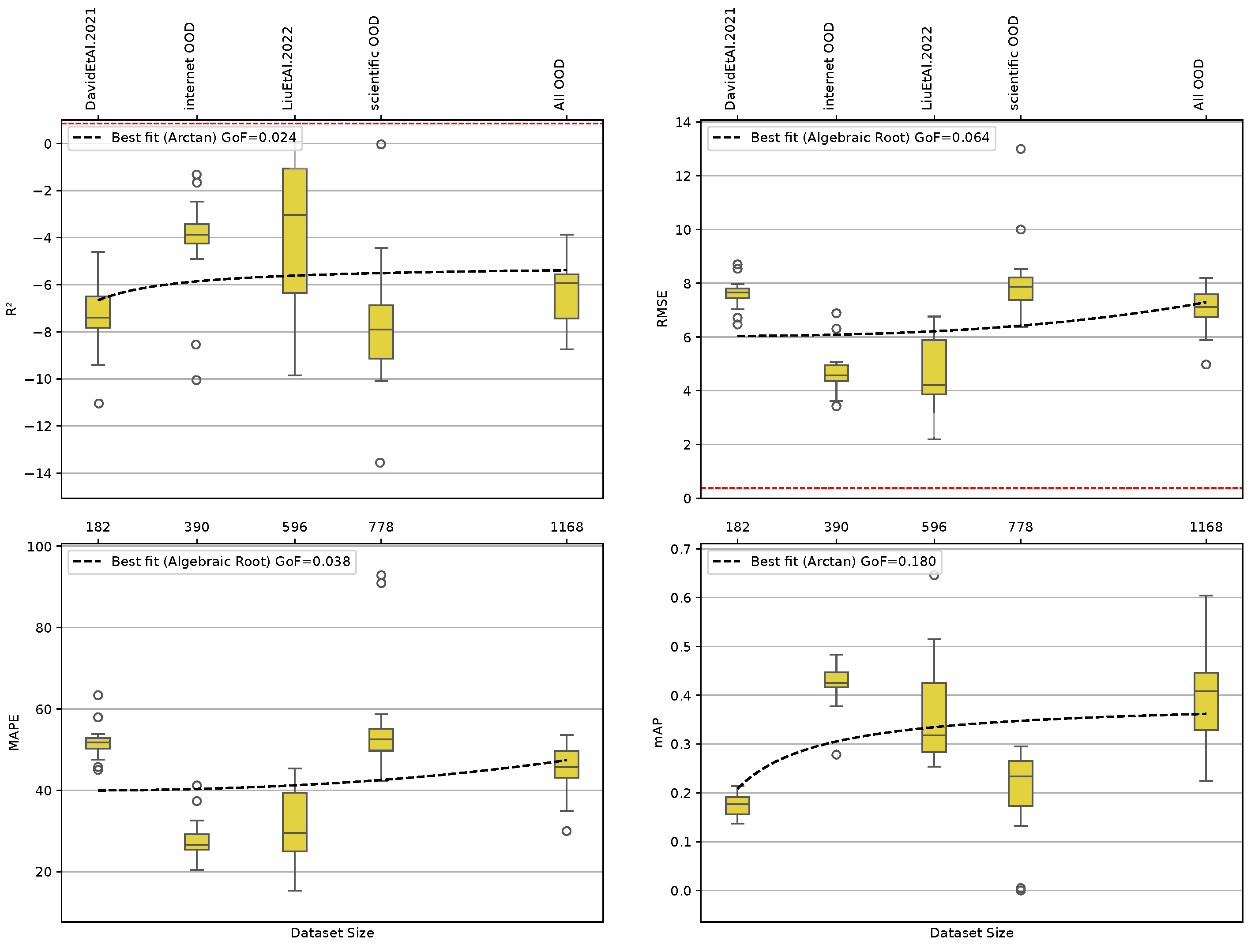
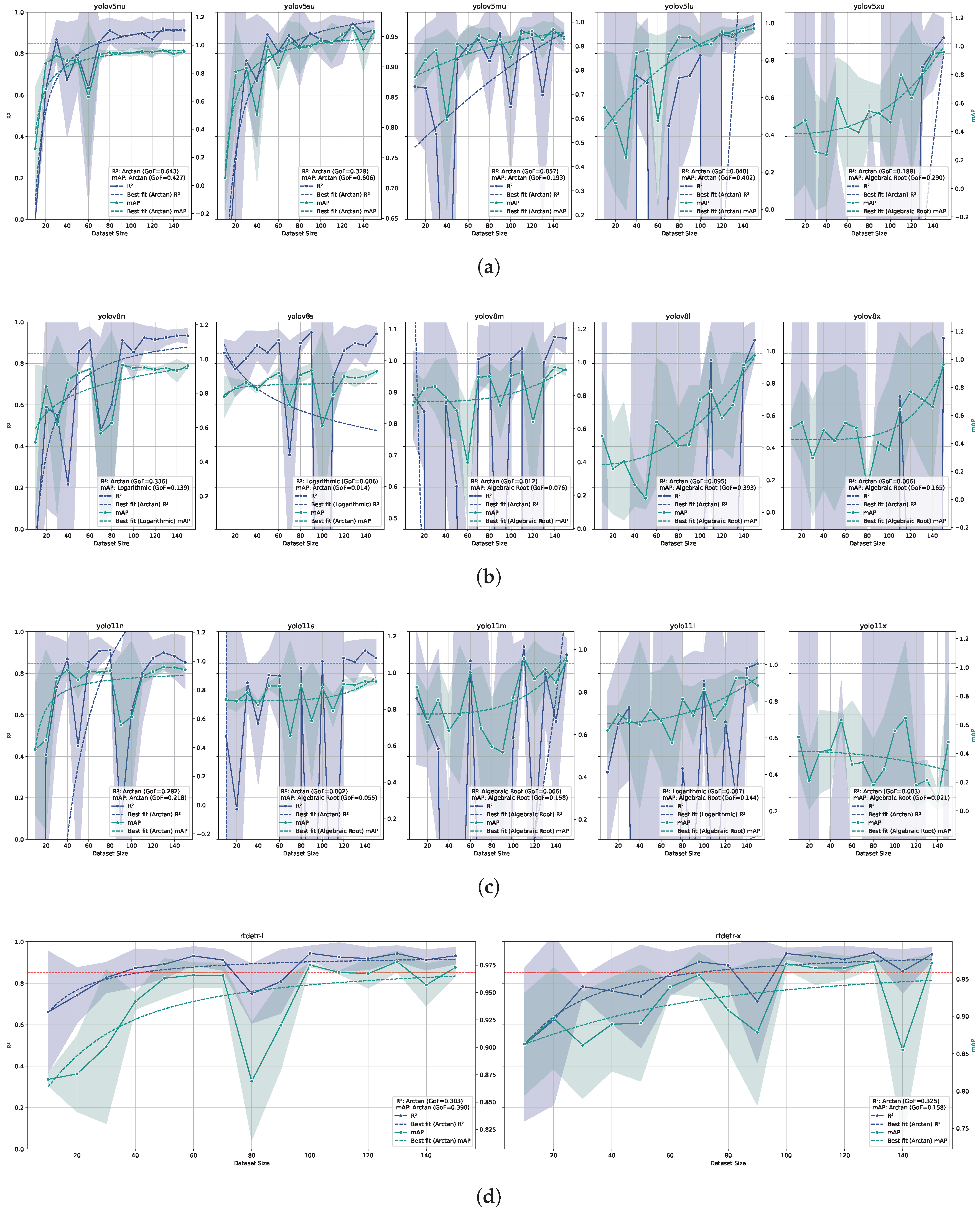
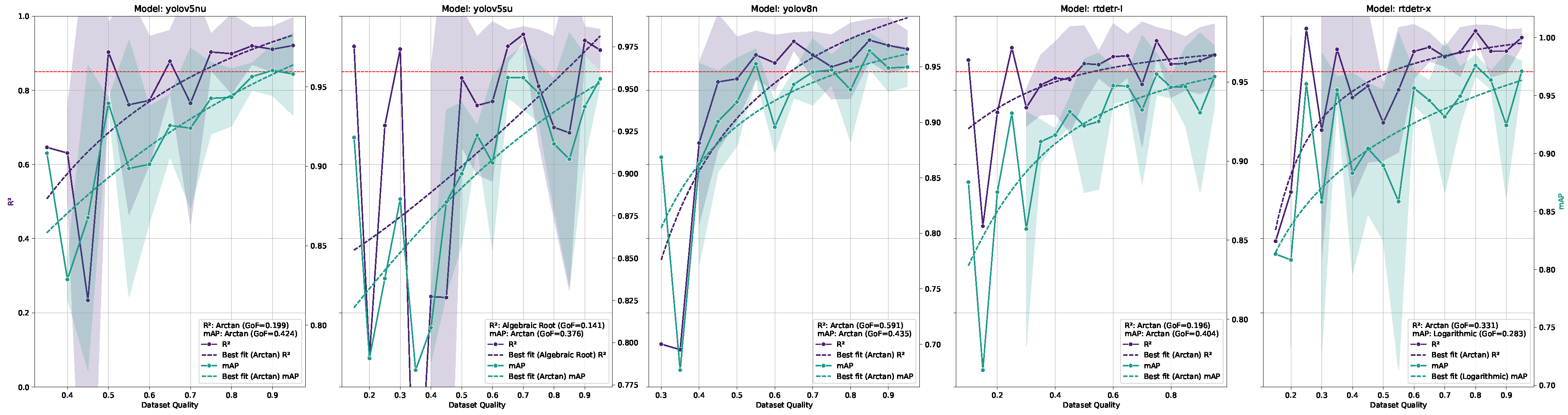
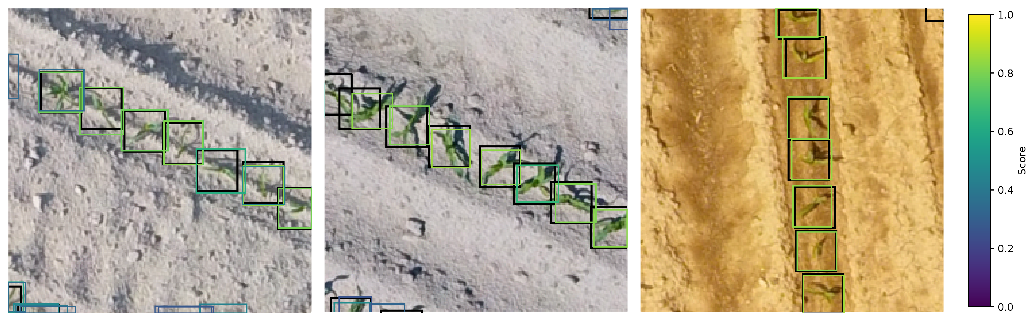
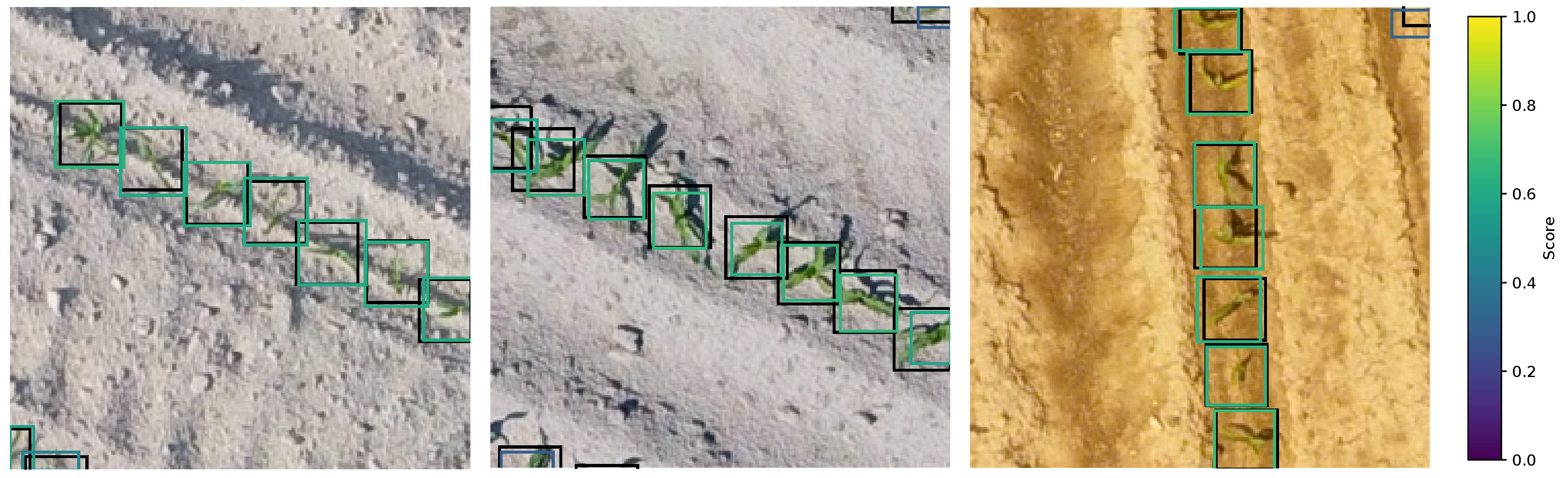
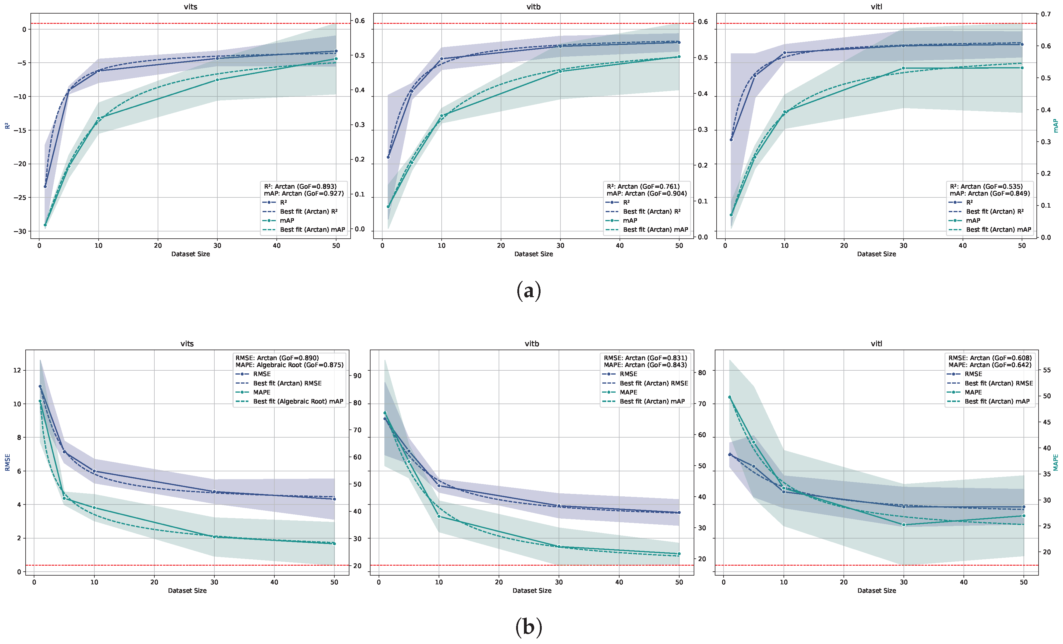
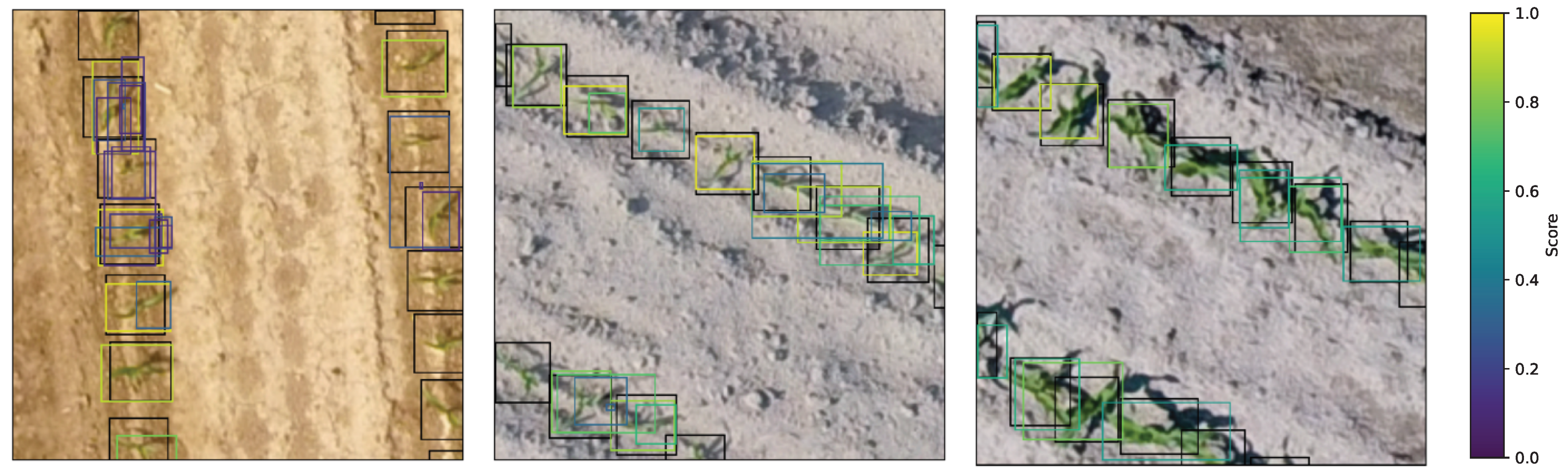
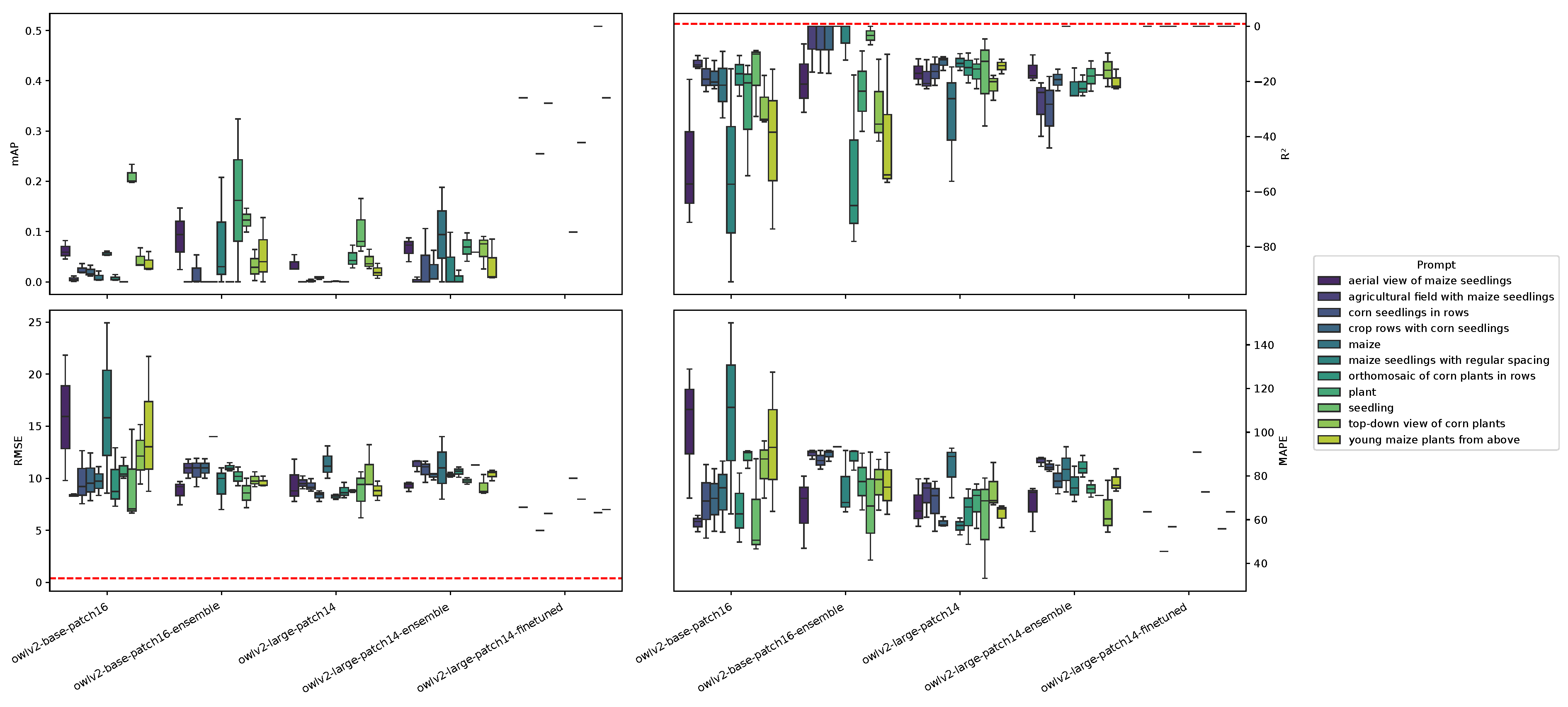
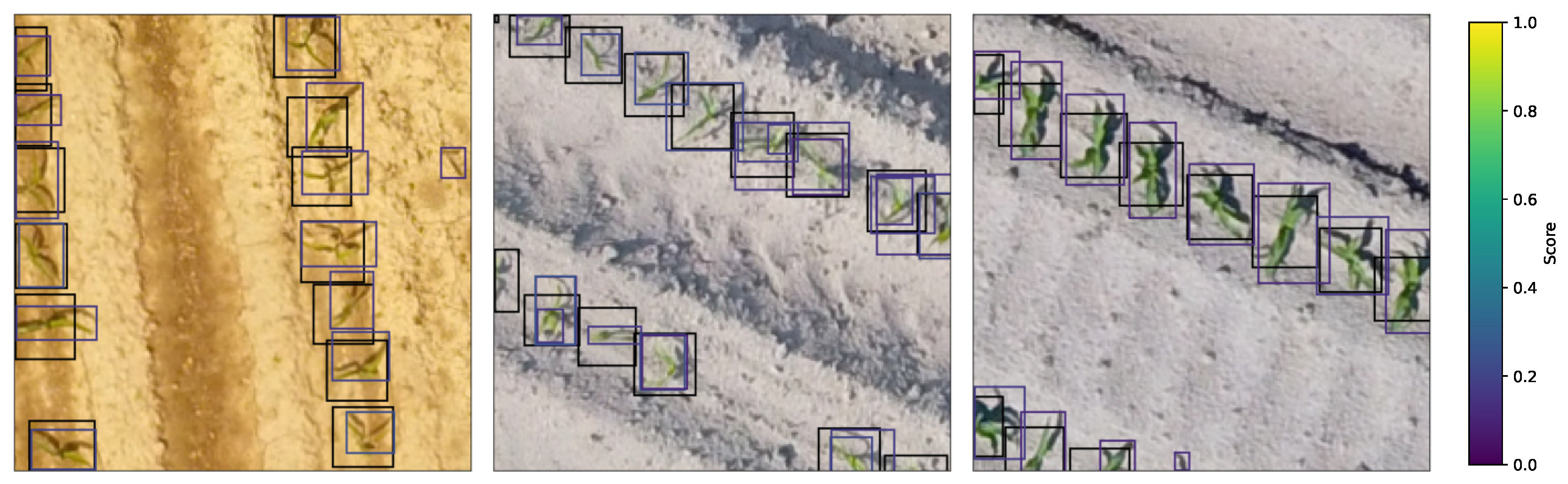
Disclaimer/Publisher’s Note: The statements, opinions and data contained in all publications are solely those of the individual author(s) and contributor(s) and not of MDPI and/or the editor(s). MDPI and/or the editor(s) disclaim responsibility for any injury to people or property resulting from any ideas, methods, instructions or products referred to in the content. |
© 2025 by the authors. Licensee MDPI, Basel, Switzerland. This article is an open access article distributed under the terms and conditions of the Creative Commons Attribution (CC BY) license (https://creativecommons.org/licenses/by/4.0/).