Generalization Enhancement Strategies to Enable Cross-Year Cropland Mapping with Convolutional Neural Networks Trained Using Historical Samples

Abstract

Mapping agricultural fields using high-resolution satellite imagery and deep learning (DL) models has advanced significantly, even in regions with small, irregularly shaped fields. However, effective DL models often require large, expensive labeled datasets, which are typically limited to specific years or regions. This restricts the ability to create annual maps needed for agricultural monitoring, as changes in farming practices and environmental conditions cause domain shifts between years and locations. To address this, we focused on improving model generalization without relying on yearly labels through a holistic approach that integrates several techniques, including an area-based loss function, Tversky-focal loss (TFL), data augmentation, and the use of regularization techniques like dropout. Photometric augmentations helped encode invariance to brightness changes but also increased the incidence of false positives. The best results were achieved by combining photometric augmentation, TFL, and Monte Carlo dropout, although dropout alone led to more false negatives. Input normalization also played a key role, with the best results obtained when normalization statistics were calculated locally (per chip) across all bands. Our U-Net-based workflow successfully generated multi-year crop maps over large areas, outperforming the base model without photometric augmentation or MC-dropout by 17 IoU points.

1. Introduction

The ability to produce precise, field-level maps of agricultural land is crucial for understanding and managing the complex interplay between food security, land use, and environmental sustainability [1]. These maps are key to understanding farmland configurations, including the spatial distribution, quantity, morphology, and dimensions of fields, which serve as key indicators in domains such as land management [2], ecosystem monitoring [3,4], food security [5,6], and precision agriculture [7,8].

The growing need for extensive, routine, and automated mapping of crop fields is driven by the rapid evolution of global agricultural systems and food security challenges in the face of climate change. This need is especially pressing in smallholder-dominated regions of Asia and Africa, where landscapes are typically characterized by small (less than 1–2 hectares), geometrically irregular, and dynamically changing fields, often featuring heterogeneous management practices and frequent presence of trees within the fields [9,10,11].

Available global- or continental-scale cropland maps are typically coarse in resolution and produced infrequently with poor or unverified accuracy (e.g., the global data set of monthly irrigated and rainfed crop areas around the year 2000 (MIRCA2000); the Global Rain-fed, Irrigated, and Paddy Croplands (GRIPC) [12] while frequent large-scale products are usually limited to developed countries (e.g., the U.S. Cropland Data Layer (CDL) or Canadian Annual Crop Inventory [13]. The Global Food Security-support Analysis Data (GFSAD) project’s products, including the Landsat-derived Global Rainfed and Irrigated-Area Product (LGRIP30) and the Landsat-derived global cropland extent product (LGCEP30), partially address some limitations in cropland data, such as imprecise spatial locations and uncertainties in differentiating irrigated and rainfed areas. Another exception is the newly available LULC product from Dynamic World [14], with 10 m resolution and near-real-time global coverage, but the resolution of these products is still too coarse to map many cultivated areas dominated by smallholder agricultural systems.

In the context of smallholder agricultural regimes, key advances in cropland mask generation have arisen from the use of high-spatial-resolution imagery (<5 m), particularly when paired with improved revisit frequency [15]. Although the use of unsupervised methods is increasing, prompted in part by the promising results from emerging foundation models, which eliminate the necessity of annotated datasets in the training process, such as Prithvi [16] and Presto [17], supervised learning techniques still dominate the majority of research in this area. In addition to precisely identifying and mapping the locations of cultivated pixels, there is an increasing emphasis on models that can accurately delineate the geometric contours of agricultural fields, to capture their shapes and sizes, which provides crucial information on agricultural systems while enhancing the overall accuracy of the mapping process [18,19,20].

Typically, any DL model optimized for object detection or semantic segmentation can be adopted and modified for the aim of crop extent mapping. Examples include DeepLabv3+ [21], specifically designed models such as ResUNet-a [22] and HRRS-U-Net [23], and ensemble models like CCTNet [24]. A popular approach used to improve segmentation masks is multi-task training, where the delineation of field boundaries serves as an auxiliary task to aid the primary segmentation goal, commonly designed as a multi-branch network with task-specific branches and strategic fusion methodologies to improve the crop mask [25,26,27,28,29]. Complementing these methods, implementing boundary-aware loss functions has proven to be an effective strategy in refining the accuracy of field boundary detection [30]. Alternative strategies focused on field boundary delineation commonly follow a two-step process involving semantic segmentation followed by instance segmentation post-processing, as exemplified by the ultrametric contour map (UCM) approach [31]. End-to-end instance segmentation strategies, such as E2EVAP [32], and region-based CNNs, such as mask-R-CNN [33], are also used for this purpose.

Despite the promising capabilities of DL models in classifying croplands and delineating fields, consistently achieving high performance across extensive spatial and temporal scales remains a significant challenge. Notably, these models often necessitate extensive training datasets with representative samples to ensure accuracy [34,35], a requirement that is difficult to meet in smallholder systems where ground or census data are sparse or unavailable due to collection costs and other resource constraints [15,36]. Moreover, the temporal specificity of samples needed to classify seasonal crops means that, even if they are available, they are typically relevant only for the current season, thereby increasing the cost and complexity of annual crop mapping [5,37]. To address these challenges, there is a growing emphasis on reusing historical samples, either from different years or geographic locations, by employing knowledge transfer strategies to mitigate the effects of domain shift [38,39,40,41].

Domain shift in the context of agricultural mapping can be roughly categorized into two types: temporal and geographical. Temporal domain shift usually involves changes in the marginal distribution of brightness values for each band in the input samples from the source year (e.g., training year) to the target years (i.e., covariate shift) [42]. Such spectral discrepancies arising over time within the same geographic location can be attributed to a variety of factors, including year-to-year variations in agricultural practices, such as crop rotation, intercropping, and changes in crop species. Environmental changes also play a role, such as fluctuations in soil moisture levels and weather patterns and even subtle shifts in atmospheric conditions, by altering the spectral signatures of the land. These shifts lead to compromised prediction quality from one year to the next, particularly when gathering images from the same season in different years is not an option, e.g., due to cloud occlusion [31]. Geographical domain shift, on the other hand, occurs when models developed and trained in one geographic region are applied to a different region, which, besides covariate shift, can also lead to a shift resulting from the label space differing between the source and target domains [42]. This type of shift is driven by changes in the dominant landscape features and their configuration, as well as regional differences in agricultural practices, which are often influenced by local agronomic, climatic, and cultural factors. Additionally, inherent environmental variations between regions, such as soil types, climate conditions, and regional atmospheric and illumination characteristics, lead to distinct spectral signatures.

In this manuscript, we focus on addressing the challenges that the temporal domain shift poses to maintaining model accuracy and on improving the ability to reuse historical samples within the same geographic area. Our goal was to improve the ability to develop reliable, annual, high-resolution maps of cropland characteristics at regional to national scales. Research on temporal generalization and the reuse of historical data in cropland mapping has been relatively limited. The majority of existing studies adopt a pixel-based approach, relying on time-series data and typically focusing on crop-type mapping, often using conventional machine learning algorithms [37,43]. In cross-year crop mapping, common practices involve the use of measures of spectral similarity between source and target years and incorporating domain knowledge to provide contextual understanding. Both approaches are based on the premise that, despite year-to-year variations, certain spectral characteristics remain consistent and can be used to identify similar crop pixels across different years. Techniques such as spectral angle distance (SAD) [44] and Euclidean distance (ED) metrics are examples of this approach, as used in one study [45] to enhance global land cover mapping accuracy. Another study [46] used temporal features derived from domain knowledge of the crop growth cycle profiles and their spectral characteristics to improve the accuracy of crop-type classification and mapping across different years. A related approach used the local similarity between time-series spectral feature vectors from historical and target year samples as a basis for creating transferable training datasets [47]. Ref. [48] used a mixture of temporal and geographical domain adaptation by applying a phenological matching technique to adapt a U-Net, initially trained on rice and corn fields in the south-central US, for mapping these crops in the midwestern US and Northeast China. While these temporal generalization methods have shown promise, they typically require time-series data and extensive domain knowledge. To create a binary cropland mask, however, mono-temporal imagery is often sufficient, which eliminates the need for complex time-series analysis while minimizing the computational burden. These limitations have prompted us to seek alternative strategies to enhance model generalization, using a similar rationale to that of [15], who used a task-specific model called FracTAL-ResUNet [49] to improve generalization while relying on weak supervision using imperfect labels to overcome the barrier of annotation scarcity.

To improve generalization, the different aspects of a pipeline, such as data pre-processing, model architecture, loss function, optimization, and regularization techniques, play an important role. Given the lack of time-series input for phenological mapping and the desire to develop a strategy that can be plugged into any supervised segmentation pipelines, we mainly emphasize input pre-processing and regularization techniques.

Input normalization is a standard pre-processing procedure in DL models, intended to standardize input features’ magnitude to enhance training. Common normalization methods include z-value standardization and min–max normalization, typically applied per band across the entire training dataset [50,51]. Since the input only interacts with the weights of the initial network layer, the impact of input normalization on model generalization has not yet been fully explored [52], and many research papers fail to adequately document the procedure, while only a few studies have directly addressed the effects of normalization on model output and generalizability. Pelletier et al. [53] investigated various normalization methods for time-series data in remote sensing. They observed that the z-value, calculated per time stamp or for the entire time series, could distort temporal profiles and obscure vegetation differences. To counter these limitations, they proposed a global feature min/max normalization using the 2% and 98% percentiles, which better preserved temporal profile shapes. There have also been attempts to remove local trends. For instance, Nguyen et al. [54] used patches of the Landsat 8 time series, normalized by mean-centering each band based on the pixel values for each local tile, to map paddy fields at the pixel level.

Image augmentation is another standard procedure used to increase the training dataset by creating new samples through the transformation of the original samples. This procedure can also act as a regularizer by increasing the variability of the dataset. Many transformations have been introduced in the literature, ranging from weak spatial transformations, such as cropping, uniform scaling, and different types of flip and rotation that preserve the topology of the image, through to stronger transformations that do not preserve topology, including image erasing and mixing strategies. There are also photometric augmentations that act on the brightness values of each pixel to make the model invariant to color and contrast changes, forcing it to rely more on shape clues rather than spectral information [55]. This form of augmentation may be particularly effective for improving temporal generalizability, as variability in illumination is a large source of domain shift [56].

Dropout [57] works by temporarily disabling some neurons in a network layer during training and is determined using a rate that specifies the probability of an individual neuron being deactivated. This approach reduces certain pathways’ dominance and prevents co-adaptation among neurons, acting as a regularizer that decreases overfitting and simplifies the network structure, which has been found to be particularly useful in deep neural networks (DNNs) that have dense layers with numerous parameters or smaller training datasets [58]. However, it may not be ideal for convolutional neural networks (CNNs), in which maintaining the spatial structure of the input is crucial, and applying standard dropout can disrupt spatial coherence due to its random deactivation of individual neurons. Spatial Dropout [59] addresses this by deactivating entire feature maps from the output of the previous layer, thus preserving the spatial coherence of the network’s activations. As a regularizer, dropout is applied exclusively during training, with all neurons being active during inference (or the model’s evaluation phase). The dropout concept inspired several adaptations for different purposes. Monte Carlo dropout [60], a Bayesian method for variational inference, employs dropout layers not only during training but also during inference to approximate the uncertainty in model predictions [61]. By using dropout during inference, multiple predictions are made with varying network configurations, leading to a distribution of outputs. These outputs are then aggregated (by averaging or majority voting) to provide a robust prediction and an uncertainty measure, which is typically the class-wise standard deviation of these predictions [62]. Kendall and Gal [63] distinguish between two main types of uncertainty: aleatoric, inherent in data due to noise; and epistemic, stemming from limitations in a model’s learned knowledge due to limited training samples. Dechesne et al. [64] applied these concepts in a practical setting by developing a compound metric that merged the entropy of prediction distribution with the mutual information between the prediction and posterior over the network weights. This metric effectively assessed both aleatoric and epistemic uncertainties, which the authors used along with the prediction–reference agreement to create qualification maps for analyzing network decisions in tasks such as extracting building footprints from benchmark datasets. MC-dropout has been used to quantify the uncertainty of DL models [65] and to increase prediction robustness by improving model repeatability [66].

In this study, we introduce a novel workflow that leverages input normalization, Monte Carlo dropout (MC-dropout), and a task-specific loss function to enhance the temporal generalization capabilities of field boundary masks at a national scale. We applied these techniques to a single U-Net model as it is well-understood and widely deployed for LULC mapping [67,68], making this study highly relevant to practitioners whose goal is to repeatedly produce reliable maps with an effective model, and who may lack the time to test the broad and expanding array of architectural variations. Our focus was to enhance our ability to produce yearly cropland masks for annual crops, excluding woody crops, aligning with common practices in the literature [69,70]. The cropland masks are particularly designed to distinguish between the field interior, field edge, and non-field background classes, which improves the ability to perform post-hoc instance segmentation using the score maps for the field interior class. The approach we demonstrate here significantly reduces the reliance on extensive multi-year sample collection, or complex transfer learning strategies, marking a meaningful improvement toward cost-effective, large-scale, and annually repeatable agricultural monitoring.

2. Materials and Methods

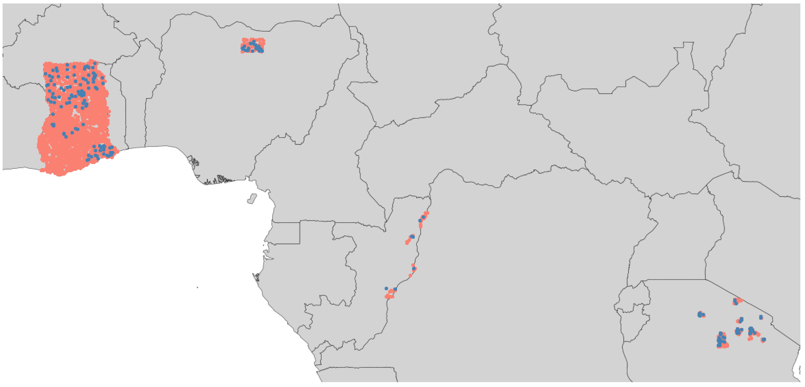
2.1. Data and Study Area

The focal region of our study was Ghana (240,000 km²), which has a diverse agricultural landscape ranging from primarily rain-fed cereal cropping in the northern savanna regions to tree-crop-dominated areas in the humid forests of the southwest [71]. Agricultural fields in Ghana are typically small, averaging less than 2 hectares in size, and characterized by heterogeneous and often indistinct field patterns [11,31]. Moreover, shifting agriculture is a common practice in this region [72]. These agronomic factors, along with the frequent cloud cover, pose significant challenges in producing multi-year cropland maps of Ghana.

For the creation of annual cropland maps spanning the years 2018–2022, we used high-resolution (3.7–4.8 m) imagery derived from daily PlanetScope imagery. These images have four bands spanning the visible and NIR spectra and were compiled using two distinct methodologies. Initially, for the year 2018, a weighted temporal averaging approach was adopted to integrate daily imagery from November or December 2018 through February 2019 into a dry season temporal composite, as detailed in [11]. These composites were structured within tiles of 2000 × 2000 pixels (0.05° × 0.05° degree, n = 8116), each with an approximate resolution of 3 m (0.000025°). For the subsequent years of 2019 to 2022, we used Planet analytic base map imagery provided by Norway’s Climate and Forests Initiative (NICFI (URL https://www.nicfi.no/)) at a resolution of 4.77 m, which is made from the best image during the time period (typically one month for 2020 onwards, and 6 months for earlier years), based on the cloud coverage and image quality using Planet’s “best-on-top” algorithm. The collection of base map mosaics covered the period from June to December 2019, as well as each November for the years 2020, 2021, and 2022. To ensure consistency across all years, these base maps were resampled to match the tiling grid and resolution used for the 2018 imagery. Additionally, to minimize boundary effects during the prediction phase, tiles were reprocessed to overlap, such that input dimensions are 2358 × 2358 pixels, with final predictions cropped to the original non-overlapping 2000 × 2000.

To train our cropland mapping model, we assembled a set of 4977 labeled images developed through manual digitization of field boundaries in the 2018 imagery, primarily as part of a prior mapping initiative [11]. This dataset includes 4229 labeled samples encompassing four different areas across the Ghanaian landscape, where annual crops such as maize are primarily produced. The dataset was further enriched with an additional 100 samples from Nigeria, 70 samples from Congo, and 578 samples from Tanzania derived from a similar procedure in 2020 to broaden the range of agronomic diversity. The samples were divided into 4781 samples for training, with the remaining 196 (4%) with the highest label quality reserved for model validation in 2018 (Figure 1).

Label polygons were converted into 200 × 200 pixel masks that distinguished between field interiors, field boundaries, and non-field areas, aligned with the dimensions of a 0.005° labeling grid. The delineation of class boundaries from the labels was executed by creating buffers around the boundaries of the original geometries with a thickness of 2 pixels.

To align with the corresponding PlanetScope-derived image chips of 224 × 224 pixels, another buffering procedure with constant values was implemented, extending the dimensions of the labels. This adjustment ensured a harmonized input to the model, accommodating the 32× downsampling factor of our encoder–decoder model, but the buffered area was masked out of the loss calculation during the training. It is noteworthy that the labels are relatively sparse, with few sample chips having more than 50% field pixels and around 20% negative chips with no crop fields (Figure 2).

2.2. Method

We developed a methodology for national-scale mapping of agricultural fields using historical samples and integrating techniques to enhance temporal generalization, in order to eliminate the need for extensive annual data collection. Central to these techniques is the choice to use input normalization and photometric augmentation, which were selected based on their ability to improve the model’s generalization capabilities.

In our normalization process, we evaluated the popular min–max normalization and z-value standardization, applying these techniques across four distinct combinations to compute the necessary statistics, taking into account both the locality of the data and the spectral bands involved. Specifically, we calculated the statistics for each chip locally across all bands (local tile across all bands, lab); for the entire dataset across all bands (global across all bands, gab); for each chip on a per-band basis (local tile per band, lpb); and for the entire dataset on a per-band basis (global per band, gpb) and investigated their effects on model performance.

To further bolster the model’s resilience against overfitting, and to enhance its adaptability to varying crop patterns, image reflectance artifacts, and domain shift, we expanded our training dataset with a combination of spatial and photometric transformations, thereby augmenting data diversity and robustness. The augmentations were applied on-the-fly with a 50% chance of occurrence, with the following order: flip, rotation between ±90°, uniform resize, and photometric transformations. Flip was randomly selected from one of the horizontal, vertical, or diagonal types, and for photometric augmentation, one option out of gamma correction, Gaussian noise, additive, and multiplicative noise was randomly selected with equal probability and applied in each epoch. We used flip, rotation, and resize to increase the input diversity and make the model invariant to size and orientation [73], as these properties are arbitrary and can vary substantially for crop fields, but given their existing widespread and standard use [15,25], we did not further analyze their effects on the model performance.

We adopted U-Net [74] for our model, chosen for its simplicity, straightforward implementation, and reliability of predictions in land-cover mapping [75,76,77]. Our U-Net variation employs a VGG-like architecture [78] with 12 convolutional layers and a 32× downsampling factor, producing feature outputs at each encoder stage of 64, 128, 256, 512, 1024, and 2048. This design strategically emphasizes the network’s width over its depth to increase the model’s capacity, accommodating the limited label dimensions of 200 × 200 pixels, thus optimizing for our specific data constraints (see Appendix A, Figure A1).

After experimenting with conventional and spatial dropout and different configurations for placing the dropout layer, we decided to use spatial dropout to regularize the model and added it to each convolution block in both the encoder and decoder subnetworks of the U-Net. We further applied MC-dropout [60] to make model prediction ensembles, which, besides providing an uncertainty measure, improved the model’s generalization power and robustness. Through experimentation, we set the number of MC trials to 10 and used a fixed dropout rate of 0.15 for the training phase and 0.1 for the inference phase.

As the output probability maps show significant variation between tiles and time points, we used the class masks to find the optimal threshold for hardening the probability maps. We iterated though a range of potential threshold values and evaluated the difference between the number of field and background pixels at each threshold, seeking to maximize this difference. We also set a condition that the background count must not exceed 10% of the total field class count. This approach helped to establish a balance between maximizing TP while keeping the FP within acceptable limits.

To refine the training of our model, we adopted several strategies. We employed focal Tversky loss [79], developed for segmentation tasks and known for its efficacy in handling imbalanced datasets and small object sizes. The process included setting a weighting scheme (α and β hyperparameters) that controlled the trade-off between false positives (FP) and false negatives (FN), as well as a focal hyperparameter (γ), which controls the model’s focus on hard-to-classify examples. We experimentally set the α and γ hyperparameters to 0.65 and 0.9, respectively, optimizing the model’s ability to learn from challenging cases and reducing the impact of easy negatives. We implemented a dynamic class-weighting scheme, based on an inverse frequentist approach, where weights are calculated on-the-fly for each class within a given input batch, as opposed to static weighting for the entire dataset. Furthermore, introducing object boundaries as a distinct class provided a straightforward yet effective technique to enhance the model’s ability to delineate individual fields. While these boundary delineations proved useful during training for field separation, they are excluded from the final predicted field mask, which has been previously shown to be effective [80].

We developed our pipeline using the PyTorch 1.9.0 library and trained our large network (157 M parameters) on an A30 GPU machine for 120 epochs with a batch size of 32. After running initial experiments on SGD, SGD with momentum, Nesterov, Adam, and Sharpness-Aware Minimization (SAM) Optimizers [81], we adopted Nesterov as the optimizer in our pipeline. The initial learning rate was set to 0.003, which was updated with a polynomial learning rate decay policy with a power of 0.8. All the free parameters of the model were chosen based on trial and error. The code for this method, available at https://github.com/agroimpacts/cnn-generalization-enhancement (accessed on 7 January 2024), will be regularly updated.

After completing the training phase, in which the model was trained using the samples that were predominantly collected from 2018 imagery, without fine-tuning on samples collected in subsequent years, we conducted a multi-faceted evaluation of the model’s predictions for the years 2018–2022. We evaluated model performance for cropland map production over a broad geographic region. To do so, we randomly selected 4 tiles of size 2358 × 2358 from the 5 years from different regions in the northern half of Ghana and manually annotated the crop fields in the resulting 20 scenes, providing an independent test set equivalent in which each scene was equivalent in extent to nearly 111 contiguous training/validation chips (see Appendix A, Figure A2). We evaluated the model predictions using a selected set of performance metrics that we used to specifically assess the degree to which input normalization, photometric augmentation, and dropout influence temporal generalizability.

The metrics included precision, reflecting the model’s accuracy in identifying field pixels; recall, measuring the ability to capture all actual field pixels; intersection over union (IOU), assessing the overlap between predicted and actual field areas for boundary accuracy; and F1-score, which harmonizes precision and recall, crucial for models dealing with imbalanced classes.

We also evaluated the performance of the cropland classification model from the spatio-temporal perspective. To achieve this, reference labels and model predictions from each year were combined to generate 32 classes, each representing the binary state of a pixel across all time points. A confusion matrix was created between the updated multi-temporal labels, and metrics were extracted for each tile.

We further explored the spectral relationships between the average reflectance of FP and FN pixels against the consistent cropland pixels over the whole temporal duration. A pixel was labeled as persistent cropland if it was consistently classified as cropland across all five years (2018–2022). The spatial confusion matrix categorized each pixel into one of four possible groups: (1) pixels that were consistently classified as cropland in both the reference and the prediction (TP); (2) pixels that were consistently classified as cropland by the model but were classified as non-crop in the reference (model hallucination; FP); (3) pixels that were classified as cropland in the reference but consistently missed by the model (model omission; FN); and (4) pixels that were non-crop in both the reference and the model predictions (TN). To investigate the spectral characteristics of classification errors, the average reflectance of each category (TP, FP, FN, TN) was analyzed using multispectral Planet imagery. For each tile and each year, pixels corresponding to TP, FP, FN, and TN were extracted from the associated Planet imagery tile.

3. Results

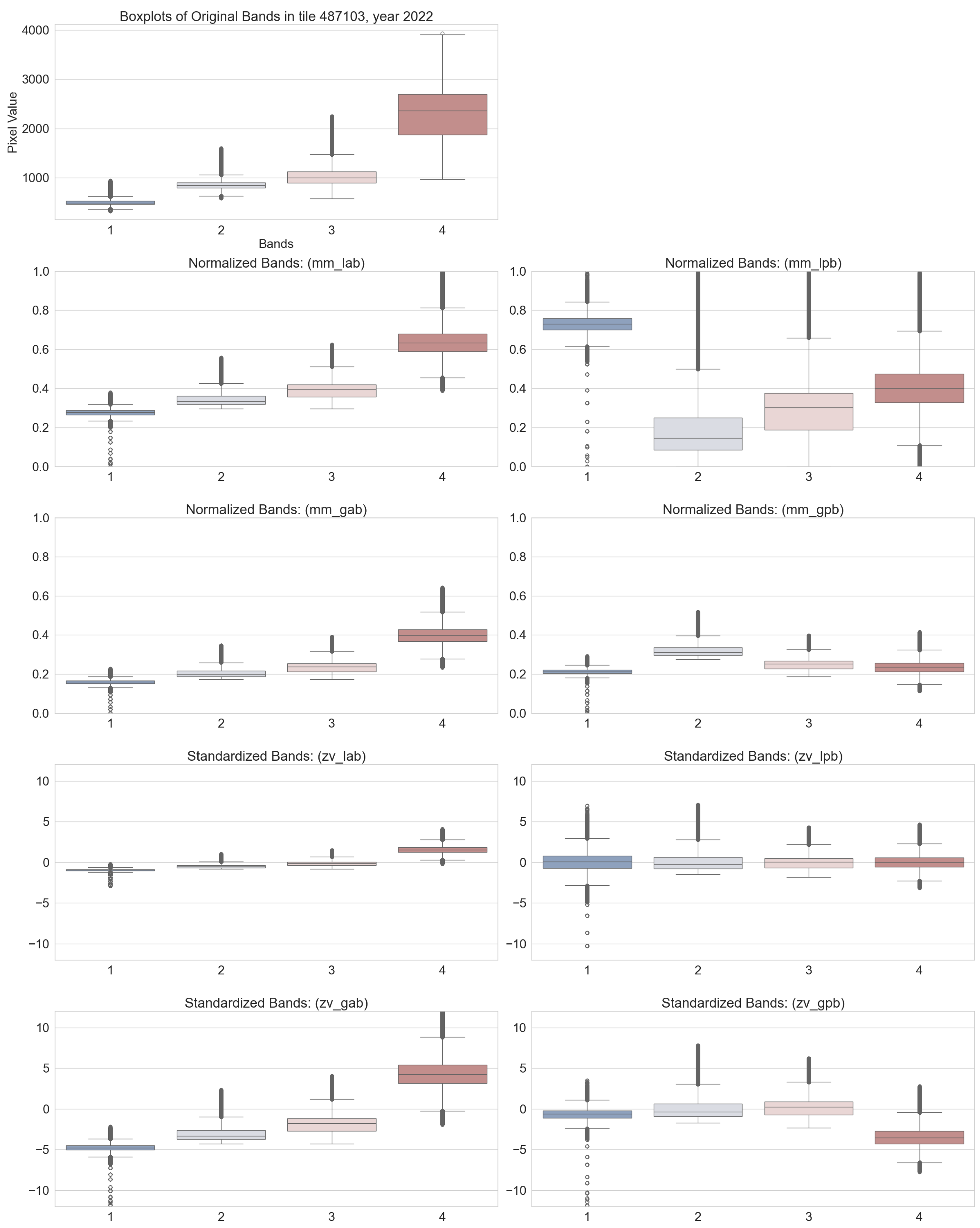
3.1. Input Normalization

An examination of spectral band distributions across this dry season period is shown in Figure 3, revealing a consistent mean within the visible (RGB) spectrum for the years 2019–2022, suggesting a relative constancy in the configuration of the major land cover types, soil exposure levels, and additional surface attributes contributing to mean spectral reflectance. The variability in the near-infrared (NIR) spectrum is likely attributable to inter-annual fluctuations in soil moisture content. The notable divergence in the brightness value distribution for the year 2018 is ascribed to variations in the data acquisition timing and the difference in the initial preprocessing method employed. The fluctuations in standard deviation highlight the underlying variability and complexity of the landscape, which could be influenced by any combination of the drivers for temporal shift (e.g., seasonal effects, soil moisture and atmospheric conditions, and the residual effects of vegetation dynamics) and the intrinsic instability of radiometric calibration in the PlanetScope product [82].

In our experiments aimed at mitigating this domain shift, we found the choice of input normalization substantially influenced the generalization capacity of the model. Comparative analyses revealed that normalization techniques using min–max scaling with “lab” and “gab” conventions yielded the best and second-best outcomes, respectively, for the tested dataset. However, no singular normalization method consistently performed best across varying temporal and geographical contexts (

Table 1. Results of accuracy assessment on the field class using a small validation set consisting of four tiles of size 2358 × 2358 pixels from 2018 to 2022 (twenty tiles in total) using the model trained on samples from 2018. All hyperparameters are fixed except the input normalization strategy. The best results are shown in bold, and the second-best results are underlined.

(a) Accuracy metric of field interior class using different normalization procedures over the multi-temporal test dataset
Normalization type		Precision		Recall	F1-score	IoU
mm-lab		74.94%		50.01%	59.99%	42.84%
mm-lpb		63.89%		52.22%	57.47%	40.32%
mm-gab		71.60%		51.53%	59.93%	42.79%
mm-gpb		83.01%		41.32%	55.18%	38.10%
zv-lab		85.42%		38.84%	53.40%	36.42%
zv-lpb		77.33%		35.73%	48.87%	32.34%
zv-gab		50.78%		56.45%	53.47%	36.49%
zv-gpb		59.21%		53.96%	56.46%	39.33%
(b) Accuracy metric of the field interior class using different normalization procedures over the multi-temporal test dataset, separated by year
Normalization type		2018	2019	2020	2021	2022
mm-lab	IoU	51.77%	42.76%	34.02%	41.44%	44.15%
	F1	68.22%	59.89%	50.77%	58.57%	61.26%
mm-lpb	IoU	49.65%	48.49%	32.06%	37.81%	36.16%
	F1	66.36%	65.31%	48.55%	54.87%	53.12%
mm-gab	IoU	50.32%	44.08%	37.69%	44.33%	38.82%
	F1	66.95%	61.19%	54.75%	61.43%	55.93%
mm-gpb	IoU	50.58%	34.15%	29.74%	39.29%	36.24%
	F1	67.18%	50.91%	45.84%	56.41%	53.20%
zv-lab	IoU	48.99%	36.09%	22.38%	36.45%	36.68%
	F1	65.76%	53.04%	36.58%	53.43%	53.67%
zv-lpb	IoU	46.98%	35.39%	17.38%	30.67%	31.18%
	F1	63.93%	52.28%	29.61%	46.95%	47.54%
zv-gpb	IoU	48.44%	42.57%	31.20%	41.15%	36.56%
	F1	65.26%	59.72%	47.56%	58.31%	53.54%
zv-gab	IoU	45.75%	36.68%	31.54%	35.91%	35.39%
	F1	62.78%	53.67%	47.96%	52.85%	52.27%
(c) Accuracy metric for the field interior class using different normalization procedures over the multi-temporal test dataset, separated by geography
Normalization type		Tile 1 (id: 487103)	Tile 2 (id: 513911)		Tile 3 (id: 513254)	Tile 4 (id: 539416)
mm-lab	IoU	45.70%	46.56%		43.31%	36.37%
	F1	62.73%	63.53%		60.44%	53.34%
mm-lpb	IoU	29.52%	47.61%		37.54%	37.04%
	F1	45.59%	64.51%		54.59%	54.05%
mm-gab	IoU	39.92%	46.47%		39.58%	46.47%
	F1	57.06%	63.45%		56.71%	63.45%
mm-gpb	IoU	40.44%	38.86%		36.73%	36.71%
	F1	57.59%	55.97%		53.73%	53.70%
zv-lab	IoU	41.80%	35.36%		35.28%	35.36%
	F1	58.96%	52.25%		52.16%	52.25%
zv-lpb	IoU	37.29%	28.10%		34.12%	28.10%
	F1	54.32%	43.88%		50.88%	43.88%
zv-gpb	IoU	29.41%	45.68%		35.28%	37.45%
	F1	45.45%	62.71%		52.15%	54.49%
zv-gab	IoU	27.08%	46.40%		36.90%	28.23%
	F1	42.62%	63.39%		53.90%	44.02%

). Our evaluation also showed that while all eight normalization techniques maintained the inter-band relational integrity (similar pairwise Pearson correlation coefficients), the “lab” and “gab” methods additionally preserved the original brightness value distributions of the imagery, whereas the “lpb” and “gpb” approaches were prone to generate more-pronounced extremes in the data values (Figure 4).

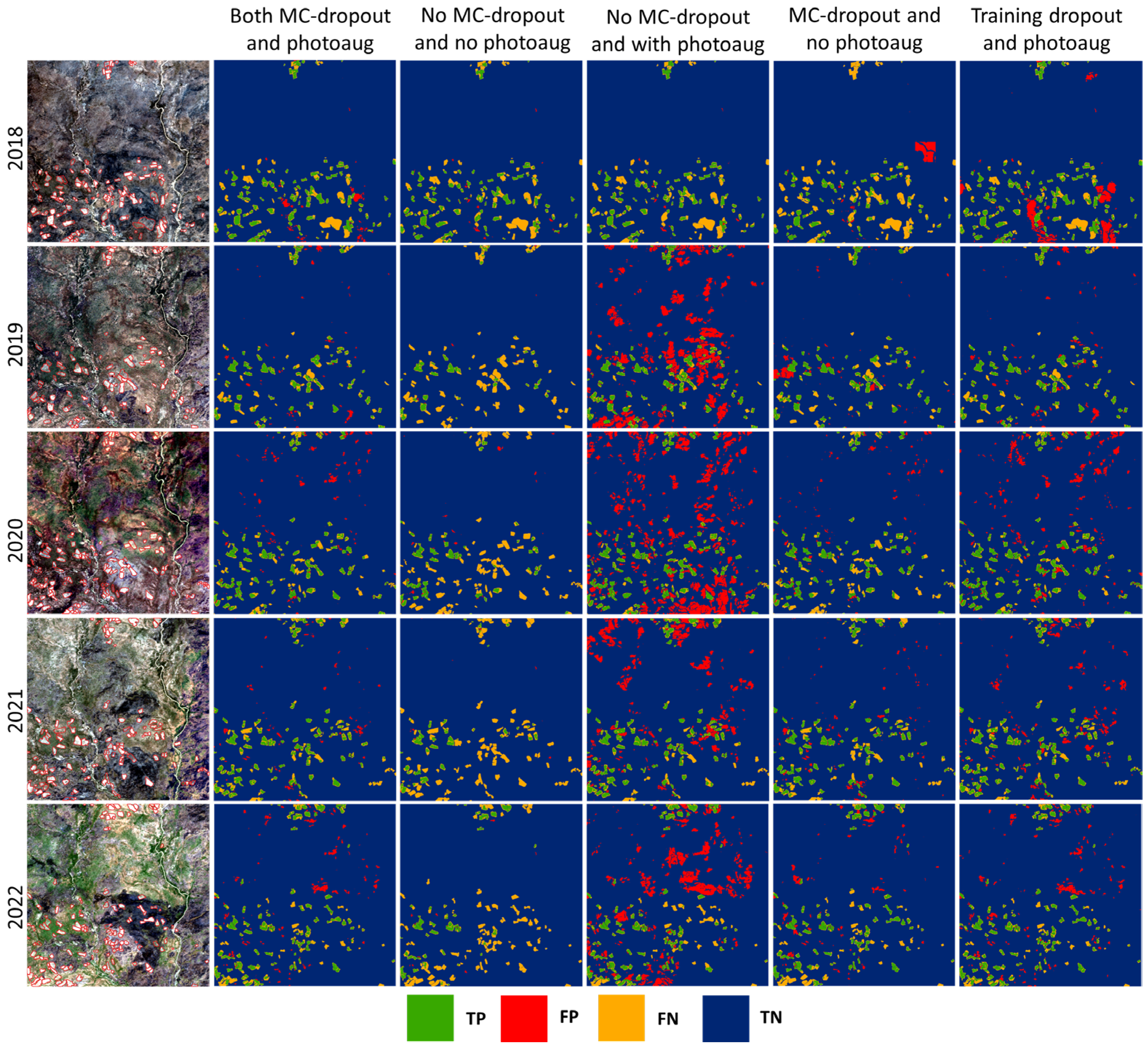
3.2. Investigating the Effects of Photometric Augmentation, MC-Dropout, Loss Function, and Model Capacity on Model Performance

Through experimentation, we observed that increasing the capacity of a U-Net model leads to improved performance. Notably, widening the model (increasing the number of channels per layer) was more effective at enhancing capacity than increasing its depth (adding more layers). However, we found that model performance plateaued at a capacity of 79 M parameters, with further increases to 158 M parameters yielding negligible gains. The non-regularized model with no dropout or photometric augmentation exhibited superior performance in generating crop maps for the year 2018. However, it was unable to accurately predict cropland distributions in subsequent years and had high rates of omission error across various regions. Incorporating photometric augmentation into the model’s training regimen improved true-positive (TP) rates but also increased the number of false positives (FP). Further integration of the dropout layers enhanced the model’s generalization capabilities, effectively reducing the incidence of FP pixels, but in the absence of photometric augmentation, using dropout markedly elevated the false-negative (FN) rate across all evaluated years. Notably, the application of MC-dropout emerged as the most effective strategy, as evidenced by the empirical results presented in

Table 2. Comparison of the effects of different combinations of photometric augmentation and dropout on the mitigation of the temporal domain shift. The values in parentheses represent the metrics before adaptive thresholding when probability scores are hardened with a fixed value of 75. The best results are shown in bold, and the second-best results are underlined.

Experiment		2018	2019	2020	2021	2022	Across All Years
No MC-dropout, no photoaug.	IoU	51.71%	23.83%	11.73%	17.70%	23.42%	25.41%
	F1	68.17%	38.49%	21.01%	30.08%	37.96%	40.52%
MC-dropout, no photoaug.	IoU	53.38% (44.71)	39.01% (18.23)	24.78% (8.12)	33.07% (14.96)	41.09% (18.82)	38.45% (20.75)
	F1	69.60% (61.79)	56.12% (30.84)	39.72% (15.03)	49.70% (26.03)	58.24% (31.68)	55.54% (34.37)
No MC-dropout, photoaug.	IoU	54.39%	32.23%	28.11%	31.13%	33.29%	34.03%
	F1	70.46%	48.75%	43.88%	47.48%	49.96%	50.79%
Only train dropout, photoaug.	IoU	51.80%	41.52%	35.45%	39.61%	43.87%	42.33%
	F1	68.25%	58.68%	52.35%	56.74%	60.98%	59.48%
Both MC-dropout, photoaug.	IoU	51.77% (50.26)	42.76% (36.08)	34.02% (25.70)	41.41% (32.72)	44.15% (40.0)	42.84% (36.97)
	F1	68.22% (66.89)	59.89% (53.02)	50.77% (40.90)	58.57% (49.31)	61.26% (57.1)	59.99% (53.98)
Both MC-dropout (conventional), photoaug.	IoU	53.39%	34.03%	24.46%	32.87%	39.80%	36.65%
	F1	69.62%	50.78%	39.31%	49.48%	56.94%	53.64%

and Figure 5 (and Appendix A, Figure A3, Figure A4 and Figure A5), indicating a marked improvement in model performance. Optimal results were achieved with a 0.15 training dropout rate and a 0.1 prediction dropout rate, with the number of MC trials set to 30. We also tried matching the histogram of the subsequent years (2019–2022) with the training year (2018) as a test phase augmentation with our best model, but this approach did not improve outcomes (Table 2 and

Table 3. Comparison of the effects of model capacity, loss function, and histogram matching against the best model with all augmentations, TF loss, and MC-dropout (both MC-dropout, photoaug.). All hyperparameters except the property under study are the same across experiments.

Experiments	Precision	Recall	F1-Score	IoU
Best model	74.94%	50.01%	59.99%	42.84%
Half capacity (width)	75.73%	48.88%	59.41%	42.26%
TFL + global weight	81.80%	32.49%	46.51%	30.30%
CE + local weight	67.88%	26.33%	37.94%	23.41%
Histogram matching	58.47%	55.13%	56.75%	39.62%

). We found that TF loss performed better than CE loss on all the tests and that calculating the class weights locally produced much lower FN compared to global class weights for weighted loss calculations. However, lowering the capacity of the model to half (e.g., 80 M trainable parameters) only slightly increased the number of FN pixels and can be used if the computation resources are limited (Table 3 and Appendix A, Figure A6).

The most substantial distinction was in the probability maps generated by the two dropout approaches, where the conventional method was overconfident in its predictions and had a much smaller range for the probability of the positive class (see Appendix A, Figure A7). However, when using the optimal hardening threshold, spatial dropout was more effective in reducing the incidence of false positives (FP) relative to traditional dropout layers. We found the optimal hardening threshold by comparing the field vs non-field histogram against the model output probabilities. Furthermore, we found that the normalization procedure also significantly influenced the model’s prediction confidence. Specifically, prediction scores generated from the mm-lab normalization and spatial MC-dropout had the widest range of probability values, providing valuable information that can help guide efforts to improve the training dataset. This feature is in addition to the utility of other layers, such as variation and mutual information, derived from the Monte Carlo trials.

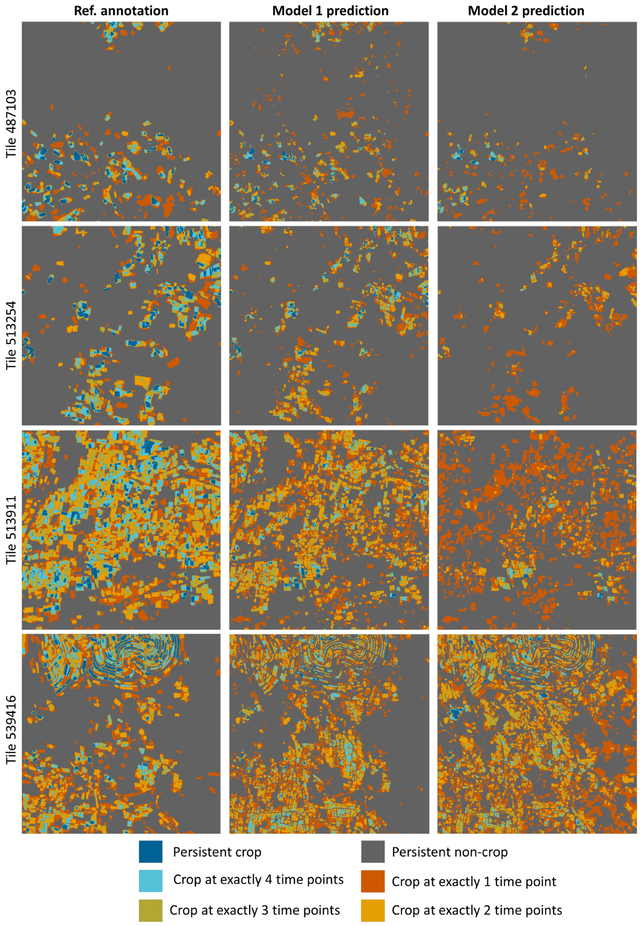
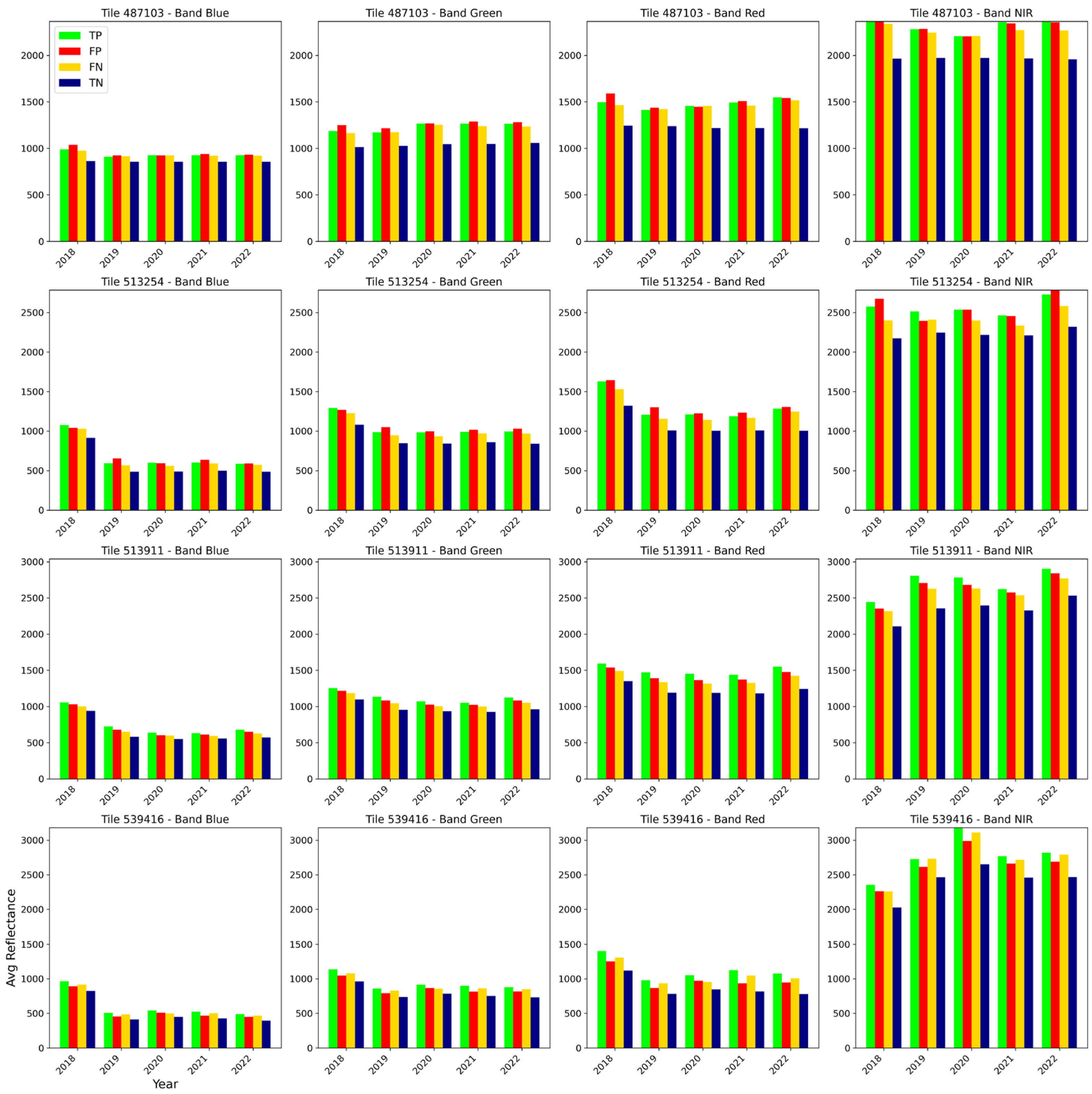
3.3. Investigating the Spatio-Temporal Consistency

For spatio-temporal consistency, we report results for the two most reliable annotations—the consistently crop and consistently non-crop pixels—as well as the average metrics for all 32 classes (

Table 4. Results from comparing model 1 (with photometric augmentation + MC-dropout) and model 2 (without photometric augmentation or MC-dropout) against the multi-temporal reference annotation, reported for each tile ID and overall.

Tile ID	Model	Category	Precision	Recall	F1-Score	IoU
487103	With MC-dropout, photoaug.	Persistent crop	87.69%	29.26%	43.87%	28.10%
		Persistent non-crop	93.82%	96.75%	95.26%	90.95%
		All categories and their subcategories	23.63%	17.18%	19%	12.05%
	W/O MC-dropout, photoaug.	Persistent crop	93.59%	11.69%	20.78%	11.60%
		Persistent non-crop	91.50%	99.58%	95.37%	91.14%
		All categories and their subcategories	15.76%	7.09%	9.87%	5.93%
513254	With MC-dropout, photoaug.	Persistent crop	81.39%	21.95%	34.58%	20.90%
		Persistent non-crop	89.51%	97.43%	93.30%	87.45%
		All categories and their subcategories	19.22%	13.89%	14.62%	9.18%
	W/O MC-dropout, photoaug.	Persistent crop	0	0	0	0
		Persistent non-crop	85.30%	99.76%	91.97%	85.13%
		All categories and their subcategories	11.45%	5.23%	9.32%	3.39%
513911	With MC-dropout, photoaug.	Persistent crop	79.53%	17.62%	28.84%	16.85%
		Persistent non-crop	63.35%	94.76%	75.93%	61.20%
		All categories and their subcategories	29.98%	18.68%	21.23%	12.55%
	W/O MC-dropout, photoaug.	Persistent crop	89.35%	3.01%	5.82%	3%
		Persistent non-crop	51.45%	96.41%	67.09%	50.48%
		All categories and their subcategories	22.64%	6.79%	6.62%	3.83%
539416	With MC-dropout, photoaug.	Persistent crop	72.65%	15.52%	25.57%	14.66%
		Persistent non-crop	82.08%	81.75%	81.92%	69.38%
		All categories and their subcategories	17.5%	13.20%	13.14%	7.91%
	W/O MC-dropout, photoaug.	Persistent crop	63.62%	19.97%	30.40%	17.93%
		Persistent non-crop	79.21%	60.57%	68.65%	52.26%
		All categories and their subcategories	17.47%	13.82%	13.47%	7.78%
Overall	With MC-dropout, photoaug.	Persistent crop	79.85%	19.72%	31.63%	18.78%
		Persistent non-crop	84.17%	93.06%	88.39%	79.20%
		All categories and their subcategories	24.21%	16.92%	18.67%	11.30%
	W/O MC-dropout, photoaug.	Persistent crop	70.25%	8.17%	14.63%	7.89%
		Persistent non-crop	78.35%	89.81%	83.96%	71.95%
		All categories and their subcategories	17.18%	8.75%	9.31%	5.78%

). To aid in visualization, the thirty-two temporal combination classes were aggregated into six parent classes: two for persistently non-crop (0 years) and persistently crop (5 years), and four for pixels classified as crop for exactly 1, 2, or 3 of the 4 years. Figure 6 illustrates the substantial improvement in segmentation consistency achieved by the best-performing model (with photometric augmentations and MC-dropout) compared to the same model without these components. The quantitative analysis in Table 4 further highlights this improvement, showing at least a twofold increase in the IoU score.

We compared the relationship between average pixel reflectance and accuracy categories regarding the consistently crop category. The results are visualized as a 4 × 4 grid of bar plots, where each row corresponds to a specific region (tile) and each column represents one of the four spectral bands (Blue, Green, Red, NIR). Within each plot, the bars show the average reflectance values for each year (2018–2022), grouped into the four accuracy categories. Each plot reveals how the spectral characteristics of cropland and non-cropland pixels differ across years, accuracy categories, and spectral bands. The structure enables comparison between correct classifications (TP, TN) and model errors (FP, FN), investigating the spectral patterns to shed light on the model’s performance and limitations.

Figure 7 shows that across all years, tiles, and bands, field pixels (TP: correctly classified field, FN: missed field) and FP pixels (non-field misclassified as field) are consistently brighter than non-field pixels (TN), particularly in the NIR and Red bands. The higher reflectance of FP pixels compared to TN highlights that the model struggles with non-field bright objects that share similar spectral and probably shape characteristics with field pixels. FN pixels (consistently missed field) generally exhibit slightly lower reflectance values than TP (consistently correctly classified field), but in some years and bands, the FN and TP values are very close, suggesting that FN pixels retain cropland spectral properties but are still misclassified.

4. Discussion

Our experimental findings regarding normalization techniques present an interesting contrast to the existing literature. While previous studies [83,84,85] advocated for band-specific normalization approaches, our results with the Ghana cropland dataset demonstrated superior performance using min–max scaling with “lab” and “gab”. While all conventions maintained inter-band relational integrity, these two also preserved the original brightness value distributions of the imagery, whereas the band-specific approaches (“lpb” and “gpb”) tended to generate more-pronounced extremes in the data values. However, no single normalization method consistently performed best across all temporal and geographical contexts, suggesting the need for context-specific optimizations. This finding highlights the challenge of temporal domain adaptation in remote sensing, where varying atmospheric conditions, seasonal effects, and sensor calibration issues can influence the effectiveness of different normalization strategies [47,86,87]. One limitation of our current study is that we did not investigate the impact of normalizing using image statistics drawn from the entire time interval, which could potentially provide more-robust normalization parameters for temporal generalization. This approach, along with a systematic investigation of normalization effectiveness across different geographical regions and temporal scales, represents an important direction for future research to establish more general guidelines for normalization in multi-temporal crop-mapping applications.

While conventional wisdom in DL often advocates for increased model capacity through deeper or wider networks, our findings suggest that such modifications yield negligible performance gains in our specific experimental context: using the U-Net architecture on the Ghana cropland dataset. We found that reducing the model capacity to 79 M parameters had minimal impact on mapping performance, showing the potential to reduce computational expense. The choice of loss function and class weighting schemes played an important role in influencing prediction accuracy, as has also been shown in numerous other studies [88,89,90]. Specifically, the TF loss function consistently outperformed CE loss, and local class weight calculations proved superior to global weighting approaches across our experiments. These findings suggest that practitioners working with similar remote sensing tasks might benefit from prioritizing the exploration of training framework components, such as loss formulations and weighting strategies, rather than focusing solely on scaling up model architecture through increasing either the model’s depth or its width. This insight is particularly relevant for operational systems where computational efficiency and model deployability are important considerations, though further research would be needed to validate these findings across different architectural families and datasets.

Our experiments demonstrated the effectiveness of MC-dropout in improving model generalization for multi-temporal crop mapping, aligning with theoretical expectations about uncertainty quantification in deep learning [65,91,92,93,94]. The implementation of MC-dropout with a 0.15 training rate and a 0.1 prediction rate, combined with 30 MC trials, showed marked improvements in model performance compared to using dropout only during training. Notably, spatial dropout proved more effective at reducing false positives compared to traditional dropout layers, though it generated probability maps with substantially higher variation in confidence levels. This increased variation presents challenges for determining optimal hardening thresholds, as we observed significant fluctuations in threshold values across both different tiles and years, which hinders the usage of spatial MC-dropout in large-scale mapping. The spatio-temporal consistency analysis also showed that our methodology substantially improved temporal generalizability, but the low metric values suggest that the improvements are insufficient to fully capture inter-annual cropland dynamics. To overcome this limitation, one strategy would be to fine-tune the model for several epochs on a small labeled dataset for the prediction year. We also need to better understand the reason behind the omission error. Our evaluation of the spectral characteristics of consistently missed or hallucinated crop pixels suggests that omission error cannot be reliably explained by spectral reflectance alone, and spatial context also needs to be considered to understand the model’s decision-making process, which is a further directive. This is also an expected behavior, as the photometric augmentations are specifically designed to reduce the model’s reliance on pixel-level reflectance, but at the same time makes it harder to explain the impact of input normalization on model performance.

The interaction between dropout and photometric augmentation revealed complex trade-offs in model regularization. While photometric augmentation improved true--positive rates, it also led to an increase in the incidence of false positives. This trade-off was partially mitigated through the integration of dropout layers, which enhanced the model’s generalization capabilities. Interestingly, our attempts to address temporal domain shift through histogram matching, where we aligned the histograms of subsequent years (2019–2022) with that of the training year (2018), proved less effective than photometric augmentation. This unexpected result might be attributed to several factors: first, histogram matching operates globally on the image level, potentially overlooking local contextual variations that are crucial for crop identification; second, the complex nature of temporal changes in agricultural landscapes might not be adequately captured by simple histogram alignment; third, photometric augmentation’s ability to simulate a wider range of potential image variations might better prepare the model for handling real-world temporal shifts.

Looking forward, several promising directions emerge for enhancing temporal generalization in crop mapping. While our current implementation focused on basic photometric augmentation, more–sophisticated approaches such as CutMix [95] and Mixup [96] warrant investigation. These methods, which create hybrid training samples by combining different images or image regions, could potentially help the model learn more-robust features across temporal domains. Additionally, exploring adaptive threshold selection methods that account for temporal and spatial variations in prediction confidence could address the challenges posed by spatial dropout’s wider probability distributions.

5. Conclusions

This work demonstrates that careful choice of pre-processing (e.g., input normalization and image augmentations) and tuning the capacity of the model accompanied by dropout regularization in both the training and prediction phases significantly improves the generalization power of the model and its capability for temporal generalization. This capability enabled a model trained primarily on samples for a single year, with imagery of a different provenance, to make high-resolution, multi-year maps of field boundaries in smallholder-dominated croplands at national scales, an important requirement for agricultural monitoring. Although the resulting maps still have some notable omission errors in each year, these errors were substantially reduced by the techniques used here, and more closely captured the inter-annual distribution of crop fields. The remaining errors may be further reduced by fine-tuning with a small number of labels collected for each year [15], targeted using the uncertainty information provided by the MC trials, with the possibility of auto-generating labels from regions with low prediction uncertainty.

References

1. Ajadi, O.A.; Barr, J.; Liang, S.-Z.; Ferreira, R.; Kumpatla, S.P.; Patel, R.; Swatantran, A. Large-scale crop type and crop area mapping across Brazil using synthetic aperture radar and optical imagery. Int. J. Appl. Earth Obs. Geoinf. 2021, 97, 102294. [Google Scholar] [CrossRef]
2. Bhosle, K.; Musande, V. Evaluation of Deep Learning CNN Model for Land Use Land Cover Classification and Crop Identification Using Hyperspectral Remote Sensing Images. J. Indian Soc. Remote Sens. 2019, 47, 1949–1958. [Google Scholar] [CrossRef]
3. Burkhard, B.; Kroll, F.; Nedkov, S.; Müller, F. Mapping ecosystem service supply, demand and budgets. Ecol. Indic. 2012, 21, 17–29. [Google Scholar] [CrossRef]
4. Akbari, M.; Shalamzari, M.J.; Memarian, H.; Gholami, A. Monitoring desertification processes using ecological indicators and providing management programs in arid regions of Iran. Ecol. Indic. 2020, 111, 106011. [Google Scholar] [CrossRef]
5. Zhang, M.; Lin, H.; Wang, G.; Sun, H.; Fu, J. Mapping Paddy Rice Using a Convolutional Neural Network (CNN) with Landsat 8 Datasets in the Dongting Lake Area, China. Remote Sens. 2018, 10, 1840. [Google Scholar] [CrossRef]
6. Karthikeyan, L.; Chawla, I.; Mishra, A.K. A review of remote sensing applications in agriculture for food security: Crop growth and yield, irrigation, and crop losses. J. Hydrol. 2020, 586, 124905. [Google Scholar] [CrossRef]
7. Mazzia, V.; Comba, L.; Khaliq, A.; Chiaberge, M.; Gay, P. UAV and Machine Learning Based Refinement of a Satellite-Driven Vegetation Index for Precision Agriculture. Sensors 2020, 20, 2530. [Google Scholar] [CrossRef]
8. Khan, S.; Tufail, M.; Khan, M.T.; Khan, Z.A.; Anwar, S. Deep learning-based identification system of weeds and crops in strawberry and pea fields for a precision agriculture sprayer. Precis. Agric. 2021, 22, 1711–1727. [Google Scholar] [CrossRef]
9. Lambert, M.-J.; Traoré, P.C.S.; Blaes, X.; Baret, P.; Defourny, P. Estimating smallholder crops production at village level from Sentinel-2 time series in Mali’s cotton belt. Remote Sens. Environ. 2018, 216, 647–657. [Google Scholar] [CrossRef]
10. Jin, Z.; Azzari, G.; You, C.; Di Tommaso, S.; Aston, S.; Burke, M.; Lobell, D.B. Smallholder maize area and yield mapping at national scales with Google Earth Engine. Remote Sens. Environ. 2019, 228, 115–128. [Google Scholar] [CrossRef]
11. Estes, L.D.; Ye, S.; Song, L.; Luo, B.; Eastman, J.R.; Meng, Z.; Zhang, Q.; McRitchie, D.; Debats, S.R.; Muhando, J.; et al. High Resolution, Annual Maps of Field Boundaries for Smallholder-Dominated Croplands at National Scales. Front. Artif. Intell. 2022, 4, 744863. [Google Scholar] [CrossRef] [PubMed]
12. Salmon, J.M.; Friedl, M.A.; Frolking, S.; Wisser, D.; Douglas, E.M. Global rain-fed, irrigated, and paddy croplands: A new high resolution map derived from remote sensing, crop inventories and climate data. Int. J. Appl. Earth Obs. Geoinf. 2015, 38, 321–334. [Google Scholar] [CrossRef]
13. Waldner, F.; Fritz, S.; Di Gregorio, A.; Defourny, P. Mapping Priorities to Focus Cropland Mapping Activities: Fitness Assessment of Existing Global, Regional and National Cropland Maps. Remote Sens. 2015, 7, 7959–7986. [Google Scholar] [CrossRef]
14. Brown, C.F.; Brumby, S.P.; Guzder-Williams, B.; Birch, T.; Hyde, S.B.; Mazzariello, J.; Czerwinski, W.; Pasquarella, V.J.; Haertel, R.; Ilyushchenko, S.; et al. Dynamic World, Near real-time global 10 m land use land cover mapping. Sci. Data 2022, 9, 251. [Google Scholar] [CrossRef]
15. Wang, S.; Waldner, F.; Lobell, D.B. Unlocking Large-Scale Crop Field Delineation in Smallholder Farming Systems with Transfer Learning and Weak Supervision. Remote Sens. 2022, 14, 5738. [Google Scholar] [CrossRef]
16. Jakubik, J.; Roy, S.; Phillips, C.E.; Fraccaro, P.; Godwin, D.; Zadrozny, B.; Szwarcman, D.; Gomes, C.; Nyirjesy, G.; Edwards, B.; et al. Foundation Models for Generalist Geospatial Artificial Intelligence. arXiv 2023, arXiv:2310.18660. [Google Scholar]
17. Tseng, G.; Cartuyvels, R.; Zvonkov, I.; Purohit, M.; Rolnick, D.; Kerner, H. Lightweight, Pre-Trained Transformers for Remote Sensing Timeseries. arXiv 2023, arXiv:2304.14065. [Google Scholar]
18. Xie, B.; Zhang, H.K.; Xue, J. Deep Convolutional Neural Network for Mapping Smallholder Agriculture Using High Spatial Resolution Satellite Image. Sensors 2019, 19, 2398. [Google Scholar] [CrossRef]
19. Sharifi, A.; Mahdipour, H.; Moradi, E.; Tariq, A. Agricultural Field Extraction with Deep Learning Algorithm and Satellite Imagery. J. Indian Soc. Remote Sens. 2022, 50, 417–423. [Google Scholar] [CrossRef]
20. Tetteh, G.O.; Schwieder, M.; Erasmi, S.; Conrad, C.; Gocht, A. Comparison of an Optimised Multiresolution Segmentation Approach with Deep Neural Networks for Delineating Agricultural Fields from Sentinel-2 Images. PFG J. Photogramm. Remote Sens. Geoinf. Sci. 2023, 91, 295–312. [Google Scholar] [CrossRef]
21. Du, Z.; Yang, J.; Ou, C.; Zhang, T. Smallholder Crop Area Mapped with a Semantic Segmentation Deep Learning Method. Remote Sens. 2019, 11, 888. [Google Scholar] [CrossRef]
22. Diakogiannis, F.I.; Waldner, F.; Caccetta, P.; Wu, C. ResUNet-a: A deep learning framework for semantic segmentation of remotely sensed data. ISPRS J. Photogramm. Remote Sens. 2020, 162, 94–114. [Google Scholar] [CrossRef]
23. Xie, D.; Xu, H.; Xiong, X.; Liu, M.; Hu, H.; Xiong, M.; Liu, L. Cropland Extraction in Southern China from Very High-Resolution Images Based on Deep Learning. Remote Sens. 2023, 15, 2231. [Google Scholar] [CrossRef]
24. Wang, H.; Chen, X.; Zhang, T.; Xu, Z.; Li, J. CCTNet: Coupled CNN and Transformer Network for Crop Segmentation of Remote Sensing Images. Remote Sens. 2022, 14, 1956. [Google Scholar] [CrossRef]
25. Wang, Y.; Ding, W.; Zhang, R.; Li, H. Boundary-Aware Multitask Learning for Remote Sensing Imagery. IEEE J. Sel. Top. Appl. Earth Obs. Remote Sens. 2021, 14, 951–963. [Google Scholar] [CrossRef]
26. Shunying, W.; Ya’nan, Z.; Xianzeng, Y.; Li, F.; Tianjun, W.; Jiancheng, L. BSNet: Boundary-semantic-fusion network for farmland parcel mapping in high-resolution satellite images. Comput. Electron. Agric. 2023, 206, 107683. [Google Scholar] [CrossRef]
27. Long, J.; Li, M.; Wang, X.; Stein, A. Delineation of agricultural fields using multi-task BsiNet from high-resolution satellite images. Int. J. Appl. Earth Obs. Geoinf. 2022, 112, 102871. [Google Scholar] [CrossRef]
28. Xu, L.; Yang, P.; Yu, J.; Peng, F.; Xu, J.; Song, S.; Wu, Y. Extraction of cropland field parcels with high resolution remote sensing using multi-task learning. Eur. J. Remote Sens. 2023, 56, 2181874. [Google Scholar] [CrossRef]
29. Luo, W.; Zhang, C.; Li, Y.; Yan, Y. MLGNet: Multi-Task Learning Network with Attention-Guided Mechanism for Segmenting Agricultural Fields. Remote Sens. 2023, 15, 3934. [Google Scholar] [CrossRef]
30. Li, M.; Long, J.; Stein, A.; Wang, X. Using a semantic edge-aware multi-task neural network to delineate agricultural parcels from remote sensing images. ISPRS J. Photogramm. Remote Sens. 2023, 200, 24–40. [Google Scholar] [CrossRef]
31. Persello, C.; Tolpekin, V.A.; Bergado, J.R.; De By, R.A. Delineation of agricultural fields in smallholder farms from satellite images using fully convolutional networks and combinatorial grouping. Remote Sens. Environ. 2019, 231, 111253. [Google Scholar] [CrossRef] [PubMed]
32. Pan, Y.; Wang, X.; Zhang, L.; Zhong, Y. E2EVAP: End-to-end vectorization of smallholder agricultural parcel boundaries from high-resolution remote sensing imagery. ISPRS J. Photogramm. Remote Sens. 2023, 203, 246–264. [Google Scholar] [CrossRef]
33. Mei, W.; Wang, H.; Fouhey, D.; Zhou, W.; Hinks, I.; Gray, J.M.; Van Berkel, D.; Jain, M. Using Deep Learning and Very-High-Resolution Imagery to Map Smallholder Field Boundaries. Remote Sens. 2022, 14, 3046. [Google Scholar] [CrossRef]
34. Schmitt, M.; Hughes, L.H.; Qiu, C.; Zhu, X.X. SEN12MS—A Curated Dataset of Georeferenced Multi-Spectral Sentinel-1/2 Imagery for Deep Learning and Data Fusion. arXiv 2019, arXiv:1906.07789. [Google Scholar] [CrossRef]
35. Fu, Y.; Shen, R.; Song, C.; Dong, J.; Han, W.; Ye, T.; Yuan, W. Exploring the effects of training samples on the accuracy of crop mapping with machine learning algorithm. Sci. Remote Sens. 2023, 7, 100081. [Google Scholar] [CrossRef]
36. Lesiv, M.; Laso Bayas, J.C.; See, L.; Duerauer, M.; Dahlia, D.; Durando, N.; Hazarika, R.; Kumar Sahariah, P.; Vakolyuk, M.; Blyshchyk, V.; et al. Estimating the global distribution of field size using crowdsourcing. Glob. Chang. Biol. 2019, 25, 174–186. [Google Scholar] [CrossRef] [PubMed]
37. Kou, W.; Shen, Z.; Liu, D.; Liu, Z.; Li, J.; Chang, W.; Wang, H.; Huang, L.; Jiao, S.; Lei, Y.; et al. Crop classification methods and influencing factors of reusing historical samples based on 2D-CNN. Int. J. Remote Sens. 2023, 44, 3278–3305. [Google Scholar] [CrossRef]
38. Hao, P.; Di, L.; Zhang, C.; Guo, L. Transfer Learning for Crop classification with Cropland Data Layer data (CDL) as training samples. Sci. Total Environ. 2020, 733, 138869. [Google Scholar] [CrossRef]
39. Van Den Broeck, W.A.J.; Goedemé, T.; Loopmans, M. Multiclass Land Cover Mapping from Historical Orthophotos Using Domain Adaptation and Spatio-Temporal Transfer Learning. Remote Sens. 2022, 14, 5911. [Google Scholar] [CrossRef]
40. Antonijević, O.; Jelić, S.; Bajat, B.; Kilibarda, M. Transfer learning approach based on satellite image time series for the crop classification problem. J. Big Data 2023, 10, 54. [Google Scholar] [CrossRef]
41. Pandžić, M.; Pavlović, D.; Matavulj, P.; Brdar, S.; Marko, O.; Crnojević, V.; Kilibarda, M. Interseasonal transfer learning for crop mapping using Sentinel-1 data. Int. J. Appl. Earth Obs. Geoinf. 2024, 128, 103718. [Google Scholar] [CrossRef]
42. Ma, Y.; Chen, S.; Ermon, S.; Lobell, D.B. Transfer learning in environmental remote sensing. Remote Sens. Environ. 2024, 301, 113924. [Google Scholar] [CrossRef]
43. Jiang, D.; Chen, S.; Useya, J.; Cao, L.; Lu, T. Crop Mapping Using the Historical Crop Data Layer and Deep Neural Networks: A Case Study in Jilin Province, China. Sensors 2022, 22, 5853. [Google Scholar] [CrossRef]
44. Kruse, F.A.; Lefkoff, A.B.; Boardman, J.W.; Heidebrecht, K.B.; Shapiro, A.T.; Barloon, P.J.; Goetz, A.F.H. The spectral image processing system (SIPS)—Interactive visualization and analysis of imaging spectrometer data. Remote Sens. Environ. 1993, 44, 145–163. [Google Scholar] [CrossRef]
45. Huang, H.; Wang, J.; Liu, C.; Liang, L.; Li, C.; Gong, P. The migration of training samples towards dynamic global land cover mapping. ISPRS J. Photogramm. Remote Sens. 2020, 161, 27–36. [Google Scholar] [CrossRef]
46. Waldner, F.; Canto, G.S.; Defourny, P. Automated annual cropland mapping using knowledge-based temporal features. ISPRS J. Photogramm. Remote Sens. 2015, 110, 1–13. [Google Scholar] [CrossRef]
47. Liu, Z.; Zhang, L.; Yu, Y.; Xi, X.; Ren, T.; Zhao, Y.; Zhu, D.; Zhu, A. Cross-Year Reuse of Historical Samples for Crop Mapping Based on Environmental Similarity. Front. Plant Sci. 2022, 12, 761148. [Google Scholar] [CrossRef] [PubMed]
48. Ge, S.; Zhang, J.; Pan, Y.; Yang, Z.; Zhu, S. Transferable deep learning model based on the phenological matching principle for mapping crop extent. Int. J. Appl. Earth Obs. Geoinf. 2021, 102, 102451. [Google Scholar] [CrossRef]
49. Diakogiannis, F.I.; Waldner, F.; Caccetta, P. Looking for Change? Roll the Dice and Demand Attention. Remote Sens. 2021, 13, 3707. [Google Scholar] [CrossRef]
50. Li, L.; Zhang, W.; Zhang, X.; Emam, M.; Jing, W. Semi-Supervised Remote Sensing Image Semantic Segmentation Method Based on Deep Learning. Electronics 2023, 12, 348. [Google Scholar] [CrossRef]
51. Zhong, Y.; Fei, F.; Liu, Y.; Zhao, B.; Jiao, H.; Zhang, L. SatCNN: Satellite image dataset classification using agile convolutional neural networks. Remote Sens. Lett. 2017, 8, 136–145. [Google Scholar] [CrossRef]
52. Huang, L.; Qin, J.; Zhou, Y.; Zhu, F.; Liu, L.; Shao, L. Normalization Techniques in Training DNNs: Methodology, Analysis and Application. IEEE Trans. Pattern Anal. Mach. Intell. 2023, 45, 10173–10196. [Google Scholar] [CrossRef]
53. Pelletier, C.; Webb, G.; Petitjean, F. Temporal Convolutional Neural Network for the Classification of Satellite Image Time Series. Remote Sens. 2019, 11, 523. [Google Scholar] [CrossRef]
54. Nguyen, T.T.; Hoang, T.D.; Pham, M.T.; Vu, T.T.; Nguyen, T.H.; Huynh, Q.-T.; Jo, J. Monitoring agriculture areas with satellite images and deep learning. Appl. Soft Comput. 2020, 95, 106565. [Google Scholar] [CrossRef]
55. Tuli, S.; Dasgupta, I.; Grant, E.; Griffiths, T.L. Are Convolutional Neural Networks or Transformers more like human vision? arXiv 2021, arXiv:2105.07197. [Google Scholar]
56. Schwonberg, M.; Bouazati, F.E.; Schmidt, N.M.; Gottschalk, H. Augmentation-based Domain Generalization for Semantic Segmentation. In Proceedings of the 2023 IEEE Intelligent Vehicles Symposium (IV), Anchorage, AK, USA, 4–7 June 2023. [Google Scholar] [CrossRef]
57. Srivastava, N.; Hinton, G.; Krizhevsky, A.; Sutskever, I.; Salakhutdinov, R. Dropout: A Simple Way to Prevent Neural Networks from Overfitting. J. Mach. Learn. Res. 2014, 15, 1929–1958. [Google Scholar]
58. Baldi, P.; Sadowski, P. The dropout learning algorithm. Artif. Intell. 2014, 210, 78–122. [Google Scholar] [CrossRef]
59. Tompson, J.; Goroshin, R.; Jain, A.; LeCun, Y.; Bregler, C. Efficient object localization using Convolutional Networks. In Proceedings of the 2015 IEEE Conference on Computer Vision and Pattern Recognition (CVPR), Boston, MA, USA, 7–12 June 2015; IEEE: Boston, MA, USA, 2015; pp. 648–656. [Google Scholar]
60. Gal, Y.; Ghahramani, Z. Dropout as a Bayesian Approximation: Representing Model Uncertainty in Deep Learning. In Proceedings of the International Conference on Machine Learning, New York, NY, USA, 19–24 June 2016; pp. 1050–1059. [Google Scholar]
61. Shridhar, K.; Laumann, F.; Liwicki, M. A Comprehensive Guide to Bayesian Convolutional Neural Network with Variational Inference. arXiv 2019, arXiv:1901.02731. [Google Scholar]
62. Kendall, A.; Badrinarayanan, V.; Cipolla, R. Bayesian SegNet: Model Uncertainty in Deep Convolutional Encoder-Decoder Architectures for Scene Understanding. arXiv 2016, arXiv:1511.02680. [Google Scholar]
63. Kendall, A.; Gal, Y. What Uncertainties Do We Need in Bayesian Deep Learning for Computer Vision? Adv. Neural Inf. Process. Syst. 2017, 30, 5574–5584. [Google Scholar]
64. Dechesne, C.; Lassalle, P.; Lefèvre, S. Bayesian U-Net: Estimating Uncertainty in Semantic Segmentation of Earth Observation Images. Remote Sens. 2021, 13, 3836. [Google Scholar] [CrossRef]
65. Mukhoti, J.; Gal, Y. Evaluating Bayesian Deep Learning Methods for Semantic Segmentation. arXiv 2018, arXiv:1811.12709. [Google Scholar]
66. Peng, L.; Wang, H.; Li, J. Uncertainty Evaluation of Object Detection Algorithms for Autonomous Vehicles. Automot. Innov. 2021, 4, 241–252. [Google Scholar] [CrossRef]
67. Song, X.; Zhou, H.; Liu, G.; Sheng-Xian Teo, B. Study of Multiscale Fused Extraction of Cropland Plots in Remote Sensing Images Based on Attention Mechanism. Comput. Intell. Neurosci. 2022, 2022, 2418850. [Google Scholar] [CrossRef] [PubMed]
68. Singh, N.J.; Nongmeikapam, K. Semantic Segmentation of Satellite Images Using Deep-Unet. Arab. J. Sci. Eng. 2023, 48, 1193–1205. [Google Scholar] [CrossRef]
69. Waldner, F.; De Abelleyra, D.; Verón, S.R.; Zhang, M.; Wu, B.; Plotnikov, D.; Bartalev, S.; Lavreniuk, M.; Skakun, S.; Kussul, N.; et al. Towards a set of agrosystem-specific cropland mapping methods to address the global cropland diversity. Int. J. Remote Sens. 2016, 37, 3196–3231. [Google Scholar] [CrossRef]
70. Potapov, P.; Turubanova, S.; Hansen, M.C.; Tyukavina, A.; Zalles, V.; Khan, A.; Song, X.-P.; Pickens, A.; Shen, Q.; Cortez, J. Global maps of cropland extent and change show accelerated cropland expansion in the twenty-first century. Nat. Food 2021, 3, 19–28. [Google Scholar] [CrossRef] [PubMed]
71. Sova, C.A.; Thornton, T.F.; Zougmore, R.; Helfgott, A.; Chaudhury, A.S. Power and influence mapping in Ghana’s agricultural adaptation policy regime. Clim. Dev. 2017, 9, 399–414. [Google Scholar] [CrossRef]
72. Kansanga, M.; Andersen, P.; Kpienbaareh, D.; Mason-Renton, S.; Atuoye, K.; Sano, Y.; Antabe, R.; Luginaah, I. Traditional agriculture in transition: Examining the impacts of agricultural modernization on smallholder farming in Ghana under the new Green Revolution. Int. J. Sustain. Dev. World Ecol. 2019, 26, 11–24. [Google Scholar] [CrossRef]
73. Sainte Fare Garnot, V.; Landrieu, L.; Giordano, S.; Chehata, N. Satellite Image Time Series Classification With Pixel-Set Encoders and Temporal Self-Attention. In Proceedings of the 2020 IEEE/CVF Conference on Computer Vision and Pattern Recognition (CVPR), Seattle, WA, USA, 13–19 June 2020; IEEE: Seattle, WA, USA, 2020; pp. 12322–12331. [Google Scholar]
74. Ronneberger, O.; Fischer, P.; Brox, T. U-Net: Convolutional Networks for Biomedical Image Segmentation. In Proceedings of the International Conference on Medical Image Computing and Computer-Assisted Intervention, Munich, Germany, 5–October 2015; pp. 234–241. [Google Scholar]
75. Karra, K.; Kontgis, C.; Statman-Weil, Z.; Mazzariello, J.C.; Mathis, M.; Brumby, S.P. Global land use/land cover with Sentinel 2 and deep learning. In Proceedings of the in 2021 IEEE international geoscience and remote sensing symposium IGARSS, Brussels, Belgium, 11–16 July 2021; pp. 4704–4707. [Google Scholar]
76. Anagnostis, A.; Tagarakis, A.C.; Kateris, D.; Moysiadis, V.; Sørensen, C.G.; Pearson, S.; Bochtis, D. Orchard Mapping with Deep Learning Semantic Segmentation. Sensors 2021, 21, 3813. [Google Scholar] [CrossRef]
77. Liu, Z.; Li, N.; Wang, L.; Zhu, J.; Qin, F. A multi-angle comprehensive solution based on deep learning to extract cultivated land information from high-resolution remote sensing images. Ecol. Indic. 2022, 141, 108961. [Google Scholar] [CrossRef]
78. Simonyan, K.; Zisserman, A. Very Deep Convolutional Networks for Large-Scale Image Recognition. arXiv 2014, arXiv:1409.1556. [Google Scholar]
79. Abraham, N.; Khan, N.M. A Novel Focal Tversky loss function with improved Attention U-Net for lesion segmentation. In Proceedings of the In 2019 IEEE 16th International Symposium on Biomedical Imaging (ISBI), Venice, Italy, 8–11 April 2019; pp. 683–687. [Google Scholar]
80. Garcia-Pedrero, A.; Lillo-Saavedra, M.; Rodriguez-Esparragon, D.; Gonzalo-Martin, C. Deep Learning for Automatic Outlining Agricultural Parcels: Exploiting the Land Parcel Identification System. IEEE Access 2019, 7, 158223–158236. [Google Scholar] [CrossRef]
81. Foret, P.; Kleiner, A.; Mobahi, H.; Neyshabur, B. Sharpness-Aware Minimization for Efficiently Improving Generalization. arXiv 2020, arXiv:2010.01412. [Google Scholar]
82. Frazier, A.E.; Hemingway, B.L. A Technical Review of Planet Smallsat Data: Practical Considerations for Processing and Using PlanetScope Imagery. Remote Sens. 2021, 13, 3930. [Google Scholar] [CrossRef]
83. Syrris, V.; Hasenohr, P.; Delipetrev, B.; Kotsev, A.; Kempeneers, P.; Soille, P. Evaluation of the Potential of Convolutional Neural Networks and Random Forests for Multi-Class Segmentation of Sentinel-2 Imagery. Remote Sens. 2019, 11, 907. [Google Scholar] [CrossRef]
84. Jeon, E.-I.; Kim, S.; Park, S.; Kwak, J.; Choi, I. Semantic segmentation of seagrass habitat from drone imagery based on deep learning: A comparative study. Ecol. Inform. 2021, 66, 101430. [Google Scholar] [CrossRef]
85. Khan, A.H.; Zafar, Z.; Shahzad, M.; Berns, K.; Fraz, M.M. Crop Type Classification using Multi-temporal Sentinel-2 Satellite Imagery: A Deep Semantic Segmentation Approach. In Proceedings of the International Conference on Robotics and Automation in Industry (ICRAI), Peshawar, Pakistan, 3–5 March 2023; pp. 1–6. [Google Scholar]
86. Wang, Z.; Zhang, H.; He, W.; Zhang, L. Phenology Alignment Network: A Novel Framework for Cross-Regional Time Series Crop Classification. In Proceedings of the 2021 IEEE/CVF Conference on Computer Vision and Pattern Recognition Workshops (CVPRW), Nashville, TN, USA, 19–25 June 2021; IEEE: Nashville, TN, USA, 2021; pp. 2934–2943. [Google Scholar]
87. Zhang, L.; Liu, Z.; Liu, D.; Xiong, Q.; Yang, N.; Ren, T.; Zhang, C.; Zhang, X.; Li, S. Crop Mapping Based on Historical Samples and New Training Samples Generation in Heilongjiang Province, China. Sustainability 2019, 11, 5052. [Google Scholar] [CrossRef]
88. Montazerolghaem, M.; Sun, Y.; Sasso, G.; Haworth, A. U-Net Architecture for Prostate Segmentation: The Impact of Loss Function on System Performance. Bioengineering 2023, 10, 412. [Google Scholar] [CrossRef] [PubMed]
89. Anaya-Isaza, A.; Mera-Jimenez, L.; Cabrera-Chavarro, J.M.; Guachi-Guachi, L.; Peluffo-Ordonez, D.; Rios-Patino, J.I. Comparison of Current Deep Convolutional Neural Networks for the Segmentation of Breast Masses in Mammograms. IEEE Access 2021, 9, 152206–152225. [Google Scholar] [CrossRef]
90. Gannod, M.; Masto, N.; Owusu, C.; Highway, C.; Brown, K.; Blake-Bradshaw, A.; Feddersen, J.; Hagy, H.; Talbert, D.; Cohen, B. Semantic Segmentation with Multispectral Satellite Images of Waterfowl Habitat. In Proceedings of the International FLAIRS Conference Proceedings, Clearwater Beach, FL, USA, 14–17 May 2023; Volume 36. [Google Scholar] [CrossRef]
91. Celikkan, E.; Saberioon, M.; Herold, M.; Klein, N. Semantic Segmentation of Crops and Weeds with Probabilistic Modeling and Uncertainty Quantification. In Proceedings of the 2023 IEEE/CVF International Conference on Computer Vision Workshops (ICCVW), Paris, France, 2–6 October 2023; IEEE: Paris, France, 2023; pp. 582–592. [Google Scholar]
92. Zhang, Z.; Dalca, A.V.; Sabuncu, M.R. Confidence Calibration for Convolutional Neural Networks Using Structured Dropout. arXiv 2019, arXiv:1906.09551. [Google Scholar]
93. Wyatt, M.; Radford, B.; Callow, N.; Bennamoun, M.; Hickey, S. Using ensemble methods to improve the robustness of deep learning for image classification in marine environments. Methods Ecol. Evol. 2022, 13, 1317–1328. [Google Scholar] [CrossRef]
94. Lakshminarayanan, B.; Pritzel, A.; Blundell, C. Simple and Scalable Predictive Uncertainty Estimation using Deep Ensembles. Adv. Neural Inf. Process. Syst. 2017, 30, 6402–6413. [Google Scholar]
95. Yun, S.; Han, D.; Chun, S.; Oh, S.J.; Yoo, Y.; Choe, J. CutMix: Regularization Strategy to Train Strong Classifiers With Localizable Features. In Proceedings of the 2019 IEEE/CVF International Conference on Computer Vision (ICCV), Seoul, Republic of Korea, 27 October–2 November 2019; IEEE: Seoul, Republic of Korea, 2019; pp. 6022–6031. [Google Scholar]
96. Zhang, H.; Cisse, M.; Dauphin, Y.N.; Lopez-Paz, D. mixup: Beyond Empirical Risk Minimization. arXiv 2018, arXiv:1710.09412. [Google Scholar]
Figure 1. The spatial distribution of training (red) and validation datasets (blue) sampled in south-southwest Africa.
Remotesensing 17 00474 g001
Figure 2. Distribution of the proportional field coverage in samples from the training dataset.
Remotesensing 17 00474 g002
Figure 3. The means and standard deviation of image brightness values in each band for each year before normalization in the test dataset.
Remotesensing 17 00474 g003
Figure 4. Distribution of the original bands and different normalization procedures for a single image tile in the year 2022. Standard deviation values of some outliers can go over ±10 for z-value standardization, which have been removed to improve the clarity of the graph.
Remotesensing 17 00474 g004
Figure 5. Spatial confusion matrix showing the effect of different combinations of spatial dropout and photometric augmentation for a sample prediction tile (487103) through the years 2018 to 2022.
Remotesensing 17 00474 g005
Figure 6. Showing the spatio-temporal consistency of model 1 (both MC-dropout and photometric augmentation) and model 2 (without MC-dropout or photometric augmentation) against the muti-temporal reference annotations.
Remotesensing 17 00474 g006
Figure 7. Relationship between average pixel reflectance for consistently crop category from the four accuracy categories reported for each tile, per band and across years.
Remotesensing 17 00474 g007