Research on Effective Radius Retrievals of Aerosol Particles Based on Dual-Wavelength Lidar

Abstract

In this study, the effective radius of aerosol particles was experimentally retrieved using a self-developed dual-wavelength atmospheric aerosol lidar. A single-valued lookup table was first established, based on the OPAC database and the Gamma size distribution model, to define the relationship between the extinction coefficient ratio and the effective radius of atmospheric aerosol particles. The extinction coefficients corresponding to the 355 nm and 1064 nm wavelengths were then calculated using the echo signals retrieved horizontally by the lidar, in conjunction with the Mie scattering lidar equation. Subsequently, the lookup table was used to retrieve the real-time effective radius of aerosol particles by inputting the extinction coefficient ratio of the two wavelengths. Finally, the retrieval results were compared with the effective radii measured by an optical particle spectrometer, which had been corrected for relative humidity. An analysis over six months showed a coefficient of determination (R²) greater than 0.83. The results demonstrated that the dual-wavelength lidar exhibits a stable performance, the retrieval method is valid, and the detection results are accurate and reliable.

1. Introduction

Aerosols are gaseous dispersion systems composed of solid or liquid particles suspended in a gas medium, with particle diameters generally ranging from 0.001 μm to 100 μm [1]. Aerosols are characterized by their complex composition, uneven distribution, and wide coverage, primarily concentrated in the lower atmosphere. They have significant impacts on global and regional climate systems, air quality, and human health. Aerosol particles participate in atmospheric radiation transfer and climate feedback processes through various mechanisms, including scattering and absorbing solar radiation, regulating cloud droplet and ice crystal formation, and altering cloud albedo [2]. The size distribution of aerosols is one of the key factors determining their optical and physical properties, and the effective radius, as a comprehensive parameter describing the aerosol size distribution, can reflect the surface area and volume characteristics of the particles. It serves as an important indicator for studying aerosol optical properties and radiative effects.

Accurate retrieval of the effective radius of aerosol particles is crucial for understanding their role in the atmospheric environment [3]. The size of aerosol particles not only influences their scattering and absorption of shortwave and longwave radiation but also directly determines their nucleation efficiency as cloud condensation nuclei (CCN) and ice nuclei (IN), thereby affecting cloud microphysical processes, fog and precipitation formation, and regional climate changes [4]. Furthermore, the size of aerosol particles plays an important role in air pollution monitoring and health effect assessments, especially in the transmission of viruses, which should not be overlooked [5].

In recent years, with the rapid development of satellite remote sensing technology, ground-based observation systems, and aerosol modeling techniques, methods for detecting aerosol size distribution and effective radius have become increasingly diverse [6]. However, due to the complexity of aerosol sources, uneven spatial distribution, and dynamic changes in particle size, there are still many technical challenges in measuring the effective radius of aerosols [7]. Therefore, further development of accurate and reliable retrieval methods, along with continuous monitoring of aerosol particle effective radius, is of great significance for improving meteorological warning and forecasting capabilities, as well as for enhancing air quality and environmental policies.

This study is based on horizontal detection and proposes an aerosol particle effective radius inversion method based on the Gamma spectrum distribution model. The method is applied to the self-developed dual-wavelength atmospheric aerosol lidar (hereafter referred to as the dual-wavelength lidar). By analyzing the retrieved real-time data and comparing it with the detections from a portable optical particle spectrometer (hereafter referred to as the particle spectrometer), the accuracy and reliability of the dual-wavelength lidar retrievals results are validated.

2. Instrument

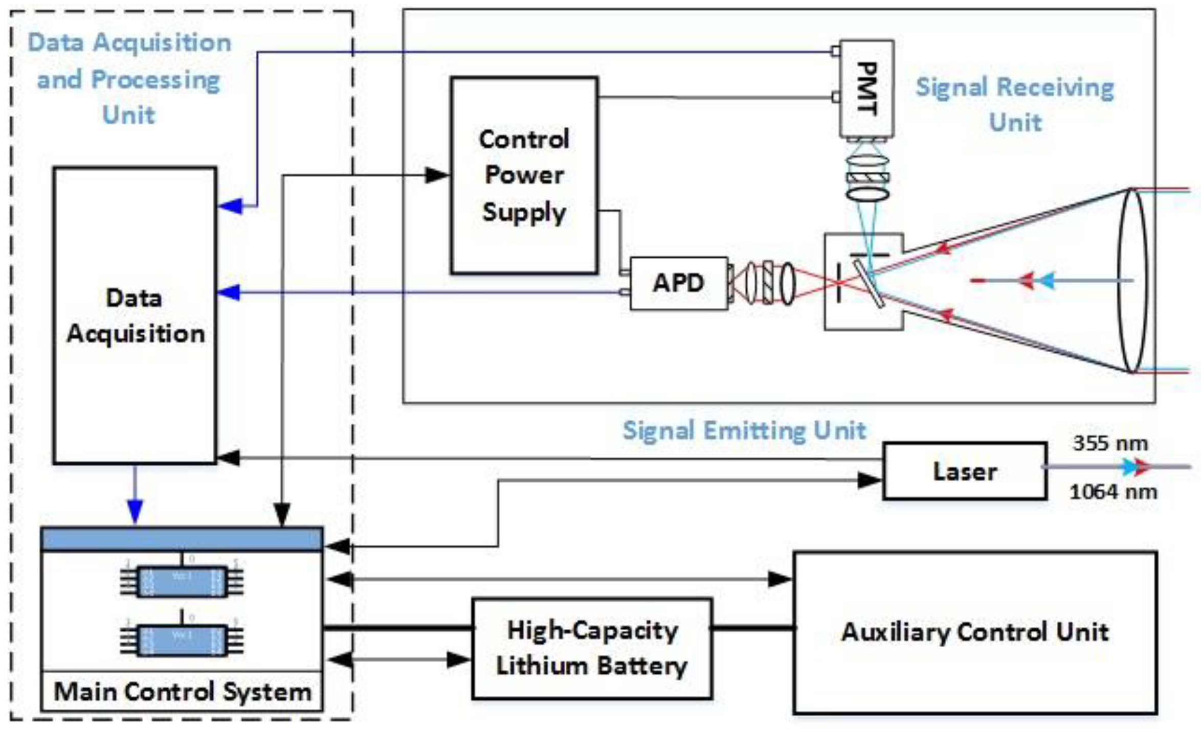
2.1. Dual-Wavelength Lidar System

The dual-wavelength lidar (Hefei CAS Gbo-Qua. Technology Co., Ltd., Hefei, China. Model GBQ L-06) used in this study employs an active optical remote sensing detection technology. As shown in Figure 1, the dual-wavelength lidar primarily consists of a signal emission unit, a signal reception unit, and a data acquisition and processing unit. In the signal emission unit, the laser beam is emitted into the atmosphere through a modulating device, where it interacts with aerosol particles. The signal reception unit captures the scattered echo signals via a receiving telescope, and the detector then converts the optical signals into electrical signals. The data acquisition and processing unit utilizes the lidar’s predefined inversion algorithm to obtain real-time aerosol microphysical parameters, such as atmospheric transmittance, particle effective radius, and particle number concentration.

The dual-wavelength lidar operates with lasers at wavelengths of 355 nm and 1064 nm. The threefold difference between these wavelengths enables the lidar to detect a wide range of effective radii of aerosol particles, thus meeting the requirements for aerosol particle retrieval across different environmental conditions. Additionally, the lidar features a compact and lightweight design, with a built-in high-performance lithium battery that supports extended outdoor detection. It outperforms similar devices in terms of adaptability to different environmental conditions and operational flexibility. The technical parameters are presented in

Table 1. The key technical parameters of dual-wavelength lidar.

Parameter Name		Channel 1	Channel 2
Overall Performance	Wavelength	355 nm	1064 nm
	Temporal Resolution	5 s~300 s	5 s~300 s
	Spatial Resolution	7.5 m	7.5 m
	Detection Range	$\ge$3 km (Under the condition of horizontal visibility $>$ 10 km)
	Weight	11.7 kg
	Power Consumption	$\le$150 W
	Battery Life	$\ge$4.8 h
Laser Transmitter Unit	Single Pulse Energy	40 μJ	40 μJ
	Laser Repetition Frequency	1 kHz	1 kHz
	Pulse Width	$<$0.6 ns	$<$0.6 ns
	Beam Expansion Gain	22 times
Signal Receiving Unit	Detector Type	PMT	APD
	Telescope Type	Transmissive
	Telescope Diameter	150 mm

.

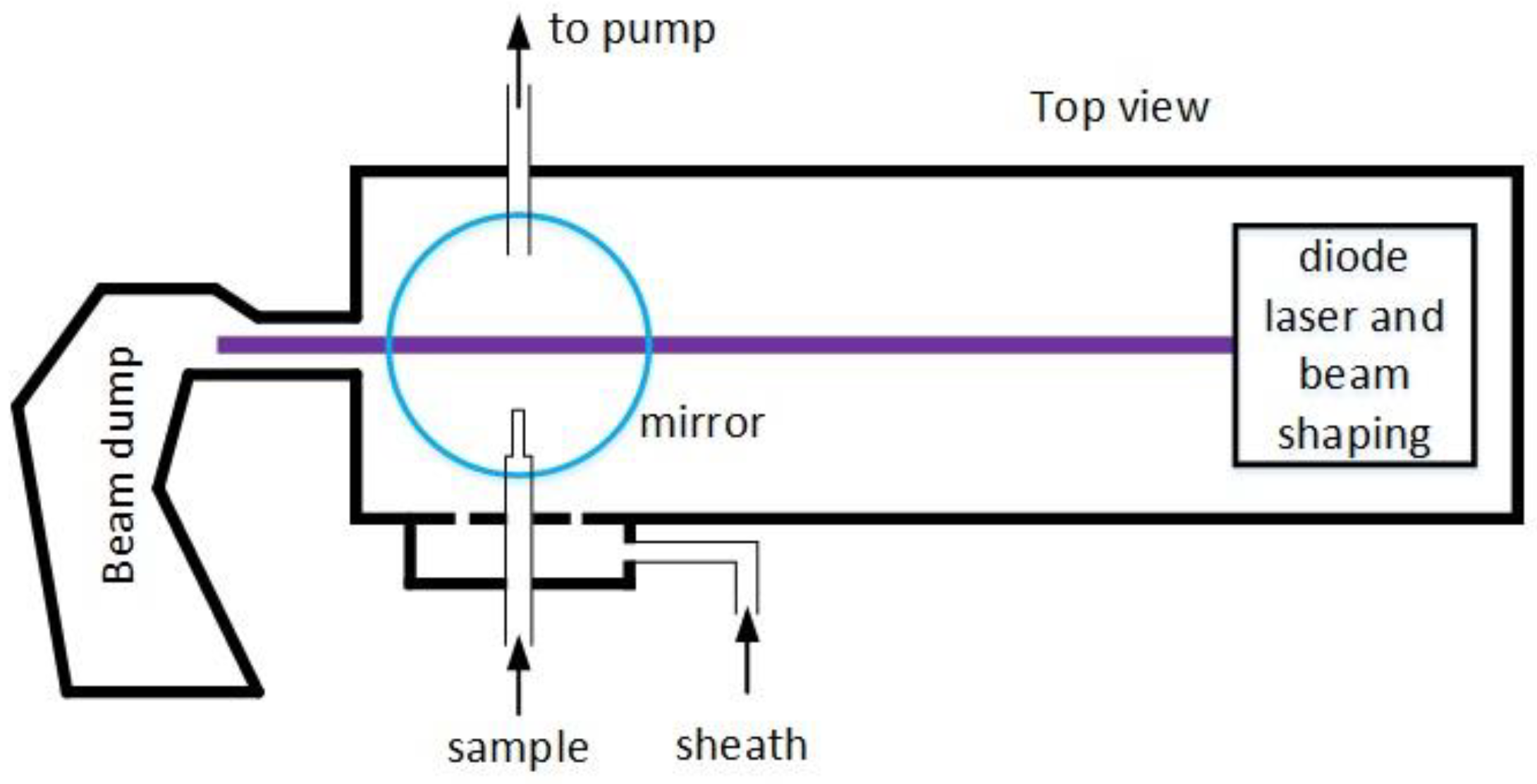
2.2. Portable Optical Particle Spectrometer

In this study, a portable optical particle spectrometer (Handix Scientific Inc., Fort Collins, CO, USA; Model POPS-1120) was used to perform a comparative validation experiment, where the particle effective radius detected by the particle spectrometer was compared with the particle effective radius retrieved by the dual-wavelength lidar to verify the validity and accuracy of the results. The reason for choosing a particle spectrometer is:

• Both the particle spectrometer and the lidar operate based on optical scattering and are influenced by the same complex refractive index, particularly its real part [8]. When the refractive index variation is minimal, these instruments can effectively reflect the consistency of aerosol optical responses.
• Although they measure different physical quantities [9], in atmospheric aerosols, where absorption effects are weak, extinction is primarily governed by scattering. Therefore, the target parameters measured by both instruments are consistent.
• Both instruments are capable of continuous 24 h field observations, enabling real-time detection of atmospheric aerosol samples within the same region. This ensures that the data originate from the same location and time, eliminating the impact of sample differences that could undermine the validity of the experiment.
• The particle spectrometer is cost-effective, requires low maintenance, and exhibits strong environmental adaptability, making it suitable for field deployments. This provides the most cost-effective solution for the present study.

The test environment is set up as shown in Figure 2; the particle spectrometer is located near the lidar’s beam path, with a horizontal distance of 1 km from the lidar. This configuration allows both instruments to simultaneously detect atmospheric aerosols in the same area under the same environmental conditions.

The particle spectrometer operates based on optical particle counting principles, detecting and measuring the diameter of particles through light scattering from individual particles. As shown in Figure 3, sample air is drawn into the detection chamber by a pump and the volume and flow rate of the intake air are measured and controlled by a laminar flow element to ensure a constant airflow. The sheath air drawn in from the branch effectively ensures that the particle flow passes stably through the laser beam region while preventing contamination of the optical components. A 405 nm wavelength laser is emitted by the laser, and as the aerosol in the sample passes through the laser beam, scattering occurs. The scattered light is collected by a spherical mirror located at the bottom of the detection chamber and focused onto a photomultiplier tube, where it is converted into an electrical signal for analysis and processing [10,11].

It should be noted that, to better adapt to high- and low-temperature environments, the particle spectrometer is equipped with an insulating outer shell, which leads to some heat accumulation within the device [8]. Although the sample gas branch of the particle spectrometer does not have filtration, heating, and drying modules, the accumulated heat causes the temperature of the sample gas to rise. Combined with the drying sheath air, this results in the relative humidity of the sample gas entering the analysis chamber being lower than that of the surrounding air. In other words, the aerosol detected by the particle spectrometer is relatively drier than that retrieved by the dual-wavelength lidar, while aerosols themselves exhibit hygroscopic growth characteristics [12,13,14]. Therefore, to more accurately compare the relationship between the particle effective radii retrieved by the dual-wavelength lidar and those detected by the particle spectrometer, the particle effective radius obtained from the particle spectrometer needs to be corrected using real-time environmental relative humidity. The specific correction method and results are presented in Section 4.1. In this study, real-time environmental relative humidity was obtained from an automatic weather station (Vaisala, Vantaa, Finland; Model WXT536), which was fixed on the same pole as the particle spectrometer, ensuring the consistency of the detected samples.

3. Aerosol Particle Effective Radius Retrieval Method

3.1. Overview of the Retrieval Process

In this study, the dual-wavelength lidar is equipped with an aerosol particle effective radius inversion algorithm, which enables real-time retrievals of the effective radius of aerosol particles in the atmosphere. The inversion process of the algorithm is divided into three main steps:

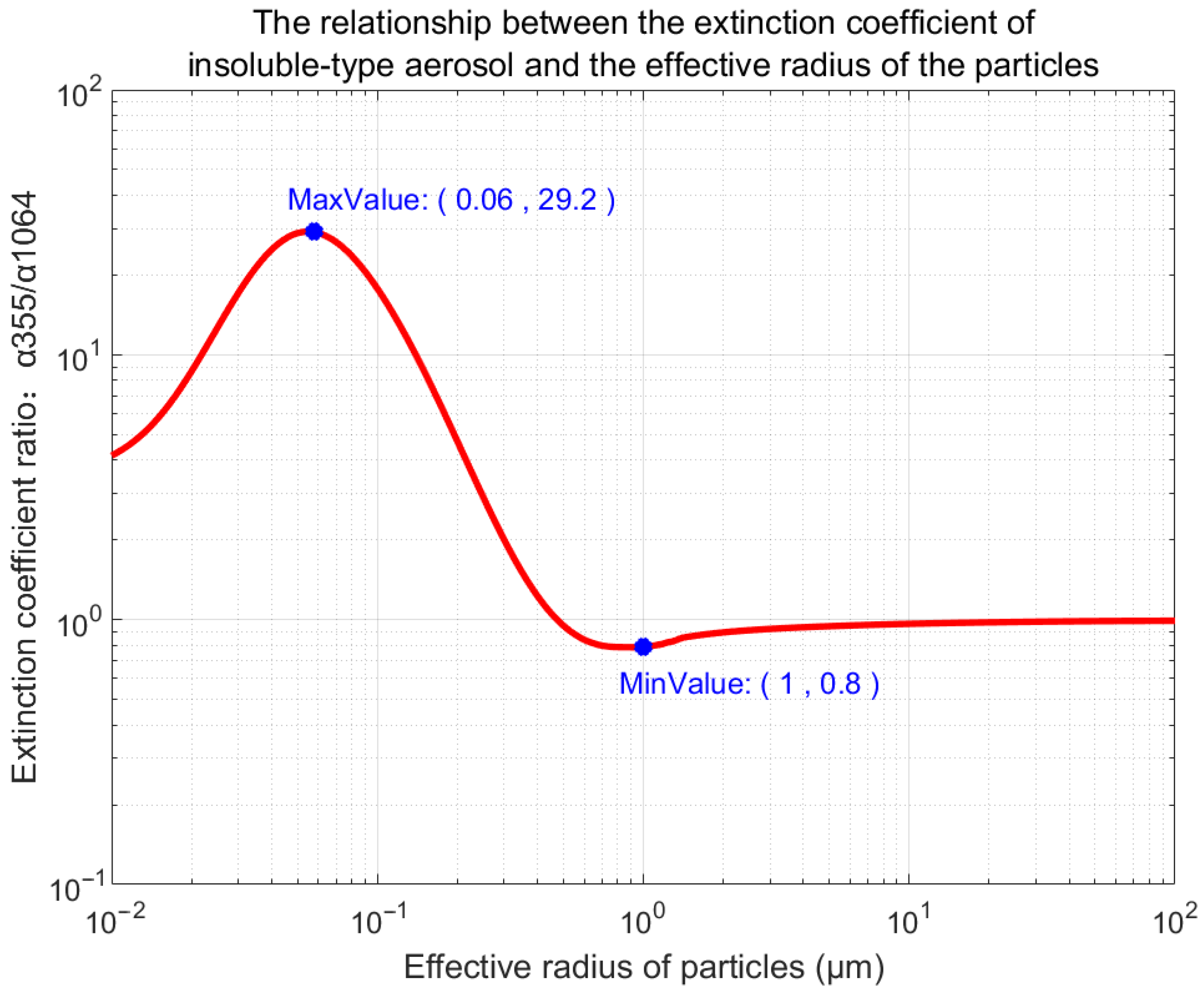
• Establishment of the extinction coefficient ratio to particle effective radius lookup table: Using the complex refractive index provided by the OPAC (Optical Properties of Aerosols and Clouds) database [15], the extinction efficiency factor of aerosol particles in the range of [0.01, 100] μm is calculated. By combining the Gamma distribution, the extinction coefficient ratio at wavelengths of 355 nm and 1064 nm can be derived. From the relationship between the extinction coefficient ratio and the particle effective radius, it is found that the extinction coefficient ratio is monotonic and unique in the range of [0.06, 1] μm, allowing for the construction of a lookup table that relates the extinction coefficient ratio to the particle effective radius within this range.
• Inversion of the measured extinction coefficient ratios for aerosol particles at two wavelengths: The real-time backscattered signals of atmospheric aerosol retrieved by the dual-wavelength lidar are used to determine the effective retrievals range of the lidar. By applying the Mie scattering lidar equation and using the slope method, the aerosol extinction coefficients at both wavelengths are calculated, leading to the calculation of the extinction coefficient ratio.
• Lookup of the real-time aerosol particle effective radius: The measured extinction coefficient ratio is combined with the extinction coefficient ratio to particle effective radius lookup table, allowing the aerosol effective radius of atmospheric aerosol particles to be determined.

3.2. Establishment of the Lookup Table for the Relationship Between Extinction Coefficient Ratio and Particle Effective Radius

3.2.1. Theoretical Basis for Establishing the Lookup Table

Common atmospheric aerosol size distributions include the Junge distribution, Gamma distribution, and log-normal distribution, which are typically characterized by volume size distributions or number size distributions. Since the optical parameters involved in this study are all related to number concentration, the number size distribution was adopted for analysis. A comparative analysis of the number concentration characteristics between the Gamma and log-normal distributions revealed that both exhibit unimodal spectral structures [16], as shown in the left panel of Figure 4. A statistical analysis of the effective radius of particles measured by the optical particle spectrometer demonstrated that under the experimental conditions of this study, the particle number proportion across different size intervals of aerosol effective radius displayed unimodal distribution characteristics. Notably, the predominant particle sizes were distributed within the [0.3–0.5] μm range, which coincides with the theoretical characteristics of the Gamma number size distribution, as illustrated in the right panel of Figure 4. These findings confirm that the Gamma distribution constitutes an appropriate selection for retrieving aerosol effective radius under the specific conditions of this investigation. Furthermore, the continuous integrability of the Gamma distribution facilitates its implementation in embedded systems [17,18,19], thereby advancing the miniaturization and portability design of dual-wavelength lidar systems. Based on these considerations, the Gamma distribution was ultimately selected for atmospheric aerosol effective radius retrieval in this study.

The mathematical expression of the Gamma distribution is given by [20,21], as follows:

$$n(r)=n_0{r}^{\mu }{e}^{-\nu r}$$

(1)

where $n(r)$ represents the aerosol particle number concentration per unit volume within a unit size interval, $r$ denotes the aerosol equivalent volume radius, $n_0$ is the number concentration parameter, $\nu$ is the slope factor, and $\mu$ is the distribution shape parameter.

The integral form of the Gamma distribution is given by [22], as follows:

$$\begin{array}{l}{M}_p={\displaystyle {\int }_0^{\infty }{r}^{p}n(r)dr}={\displaystyle {\int }_0^{\infty }{r}^p{n}_0{r}^{\mu }{e}^{-\nu r}dr}\\ \begin{array}{cc}& \end{array}={\displaystyle \frac{n_0}{v^{(p+\mu +1)}}}{\displaystyle {\int }_0^{\infty }{(\nu r)}^{(p+\mu +1)-1}{e}^{-\nu r}d(\nu r)}\\ \begin{array}{cc}& \end{array}={\displaystyle \frac{n_0}{v^{(p+\mu +1)}}}\Gamma (p+\mu +1)\end{array}$$

(2)

where $p$ represents the order of integration for the Gamma distribution, $M_p$ denotes the p-th moment integral of the Gamma distribution, and $\Gamma \left(p+\mu +1\right)=\left(p+\mu \right)!$.

Although the lidar measurements are based on the extinction effect, the experimental site in this study was located far from urban areas, where the aerosol population was dominated by insoluble particles. Moreover, no dust storms or emissions from stationary pollution sources occurred during the observation period. Under such conditions, aerosol particles can be approximately treated as spherical, with a relatively small imaginary part of the complex refractive index. Therefore, the extinction was primarily attributed to scattering. From the perspective of scattering theory, the scattering cross-section of particles is closely related to their surface area. Accordingly, the effective radius of aerosol particles can be derived using a surface-area-weighted method for spherical particles, as expressed by the following equation [23,24]:

$$R_{eff}={\displaystyle \frac{{\displaystyle {\int }_0^{\infty }\pi r^{3}n(r)dr}}{{\displaystyle {\int }_0^{\infty }\pi r^{2}n(r)dr}}}={\displaystyle \frac{{\displaystyle {\int }_0^{\infty }{r}^{3}n(r)dr}}{{\displaystyle {\int }_0^{\infty }{r}^{2}n(r)dr}}}$$

(3)

Based on Equations (2) and (3), the particle effective radius can be derived as the ratio of the third-order moment integral to the second-order moment integral of the Gamma distribution, expressed as follows:

$$\begin{array}{l}{R}_{eff}={\displaystyle \frac{{\displaystyle {\int }_0^{\infty }{r}^{3}n(r)dr}}{{\displaystyle {\int }_0^{\infty }{r}^{2}n(r)dr}}}={\displaystyle \frac{M_3}{M_2}}={\displaystyle \frac{\frac{n_0}{v^{(\mu +4)}}\Gamma (\mu +4)}{\frac{n_0}{v^{(\mu +3)}}\Gamma (\mu +3)}}\\ \begin{array}{cc}& \end{array}={\displaystyle \frac{{\nu }^{(\mu +3)}}{{\nu }^{(\mu +4)}}}\cdot {\displaystyle \frac{\Gamma (\mu +4)}{\Gamma (\mu +3)}}={\displaystyle \frac{1}{\nu }}\cdot (\mu +3)\end{array}$$

(4)

According to aerosol optical properties theory, the ratio of the extinction energy of a particle to the incident light intensity is referred to as the particle’s extinction cross-section. The ratio of the extinction cross-section to the particle’s maximum cross-sectional area is called the extinction efficiency factor, denoted as $Q_{ext}$ [25]. In real atmospheric conditions, aerosols are geometrical entities with certain size distributions and shape characteristics. Their overall optical properties are determined by the optical properties of individual particles, weighted according to the particle size distribution [26]. The formula for the extinction coefficient is as follows:

$$\alpha ={\displaystyle {\int }_{r_{min}}^{r_{max}}{Q}_{ext}\pi r^{2}n(r)dr}$$

(5)

where $[r_{min},r_{max}]$ represents the radius range of the size distribution. By substituting Equation (1) into Equation (5), we obtain the following:

$$\alpha ={\displaystyle {\int }_{r_{min}}^{r_{max}}{Q}_{ext}\pi r^2{n}_0{r}^{\mu }{e}^{-\nu r}dr}$$

(6)

The range of effective radii to be studied is selected as $[R_{eff1},R_{eff2}]$. According to Equation (4), the spectral distribution parameters corresponding to each effective radius, $\nu =(\mu +3)/R_{eff}$, can be obtained. Therefore, in Equation (6), the only unknown parameters are $n_0$ and $\mu$. When calculating the extinction coefficient ratio at two wavelengths, $n_0$ is canceled out, and it does not affect the result. At this point, the extinction coefficient ratio is independent of $n_0$. However, for computational convenience, the extinction coefficients at the two wavelengths are calculated separately. In this case, $n_0$ is not canceled out, and it can be assumed to be an arbitrary constant, for example, $n_0=1$. Once the value of $\mu$ is known, the extinction coefficient at a specified wavelength corresponding to the particle effective radius can be calculated using Equation (6), thus establishing the relationship between the particle effective radius and the extinction coefficient ratio at the two wavelengths.

3.2.2. Implementation Process for Establishing the Lookup Table

In 2023, Benli Liu and Dong Liu conducted a detailed analysis of the factors that could introduce errors in the inversion of the effective radius of atmospheric aerosol particles using a dual-wavelength method. The analysis indicated that, for insoluble aerosols, the error in the extinction coefficient ratio between the two wavelengths (355 nm and 532 nm) is minimized when the distribution shape factor ($\mu$) is set to 2 [17]. According to the OPAC database, the complex refractive indices for the wavelengths 355 nm, 532 nm, and 1064 nm are identical. Therefore, $\mu =2$ was also selected for calculations in this study. Moreover, the experimental environment for this study is located in the suburban area of a city, where insoluble aerosols predominantly exist. Thus, insoluble aerosols were also selected as the subject of analysis in this study.

As described in Section 1 of this study, the aerosol particle size range is between 0.01 μm and 100 μm. Accordingly, the range of effective particle radii selected for this study is between 0.01 μm and 100 μm. The complex refractive indices for the wavelengths 355 nm and 1064 nm can be obtained from the OPAC database, with both wavelengths having a refractive index of 1.53 − 0.008i. Based on the Mie scattering theory, the extinction efficiency factor ($Q_{ext}$) for a specified spectral distribution radius can be calculated for a given refractive index. By applying Equation (6), the extinction coefficient ratio for particle effective radii in the range of 0.01 μm to 100 μm can be derived, as shown in Figure 5.

From Figure 5, it is evident that for particle effective radii between 0.06 μm and 1 μm, the extinction coefficient ratio of the two wavelengths (355 nm and 1064 nm) monotonically decreases. This means that within the extinction coefficient ratio range of 0.8 to 29.2, there is a unique particle effective radius corresponding to each ratio value. Therefore, a lookup table for the extinction coefficient ratio as a function of particle effective radius in the range of 0.06 μm to 1 μm can be established. A statistical analysis of the measured extinction coefficient ratios from dual-wavelength lidar data revealed that most ratios are concentrated in the range of 1 to 5, accounting for over 80% of the data. The ratios within the range of 0.8 to 29.2 account for more than 99.7%. Thus, the lookup table for particle effective radii between 0.06 μm and 1 μm meets the detection requirements.

3.3. Retrieval of the Measured Extinction Coefficient Ratios at Two Wavelengths

3.3.1. Theoretical Basis for Extinction Coefficient Retrieval

The Mie scattering lidar equation is given by the following:

$$P(\mathrm{z})={\displaystyle \frac{C\beta \exp (-2{\displaystyle {\int }_{z_0}^z\alpha }d{z}^{\prime })}{z^2}}$$

(7)

where $z$ represents range; $P(\mathrm{z})$ represents the atmospheric backscattered power received by the lidar at range $z$ (W); $C$ is the lidar system constant; $\alpha$ denotes the extinction coefficient of the atmosphere at range $z$ for wavelength $\lambda$; $\beta$ is the backscatter coefficient of the atmosphere at range $z$ for wavelength $\lambda$.

By multiplying both sides of Equation (7) by the square of the range, taking the logarithm, and differentiating, the following equation is obtained:

$${\displaystyle \frac{d(\ln [P(\mathrm{z})z^2])}{dz}}={\displaystyle \frac{1}{\beta }}{\displaystyle \frac{d\beta }{dz}}-2\alpha$$

(8)

In this study, the dual-wavelength lidar employs a horizontal detection mode, from which it can be assumed that the atmosphere is homogeneously distributed. The effective detection range of the lidar is approximately 3 km. At this range, the atmospheric backscatter coefficient is considered constant, and thus, $d\beta /dz=0$. Therefore, Equation (8) can be simplified as follows:

$$\alpha =-{\displaystyle \frac{1}{2}}{\displaystyle \frac{d(\ln [P(\mathrm{z})z^2])}{dz}}$$

(9)

Equation (9) represents the calculation formula for the aerosol extinction coefficient. In this formula, the logarithm of the echo signal, after being corrected for the square of the range $\ln [P(z)z^2]$, is taken, followed by linear fitting. Half of the negative slope of the fitted curve corresponds to the measured aerosol extinction coefficient at the respective wavelength. This method is commonly referred to as the slope method.

3.3.2. Implementation Process for Extinction Coefficient Retrieval

The dual-wavelength lidar is capable of simultaneously detecting echo signals of atmospheric aerosols at two different wavelengths. Before retrieval, background and noise interference must be removed from the echo signals to reduce detection errors. The effective detection range of the lidar is then determined based on the signal-to-noise ratio. The echo signals are corrected for range using Equation (9), followed by a logarithmic transformation. This process yields two corrected signals at wavelengths of 355 nm and 1064 nm, as shown in Figure 6A, using real-time data collected by the lidar on 8 November 2022, at 22:35. Subsequently, within their respective valid detection ranges, the two corrected signals are linearly fitted, as shown in Figure 6B, to obtain their respective slopes. The slope of the 355 nm signal is −2.3008, and the slope of the 1064 nm signal is −1.0973. The extinction coefficients for the two wavelengths of the dual-wavelength lidar can then be calculated from these slopes, denoted as ${\alpha }_{355}=1.1504$ and ${\alpha }_{1064}=0.5487$, respectively. Subsequently, the extinction coefficient ratio for the two wavelengths, denoted as ${\alpha }_{355}/{\alpha }_{1064}=2.0966$, can be obtained.

At this point, by using the extinction coefficient ratio derived from the dual-wavelength lidar retrievals, and referring to the corresponding relationship between the extinction coefficient ratio and the effective particle radius, the real-time effective particle radius of atmospheric aerosols can be obtained from the lookup table. The data from Figure 6 yields an effective particle radius of 0.29 μm for the aerosols at that moment.

4. Results

To verify the validity and accuracy of the dual-wavelength lidar retrievals results, the inversion process described in Section 3 is employed to calculate the real-time effective radius of atmospheric aerosol particles and compare it with the detections from the particle spectrometer.

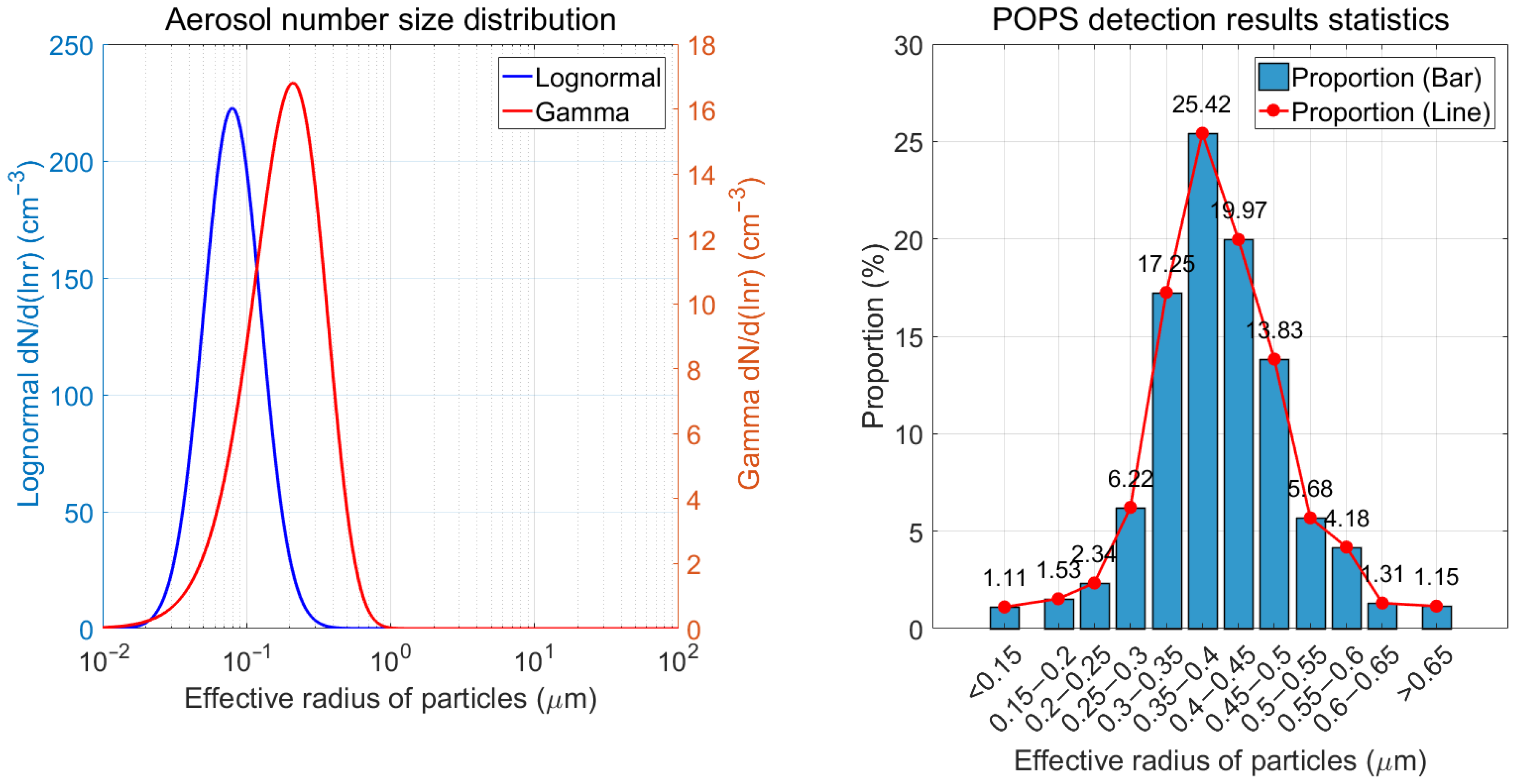
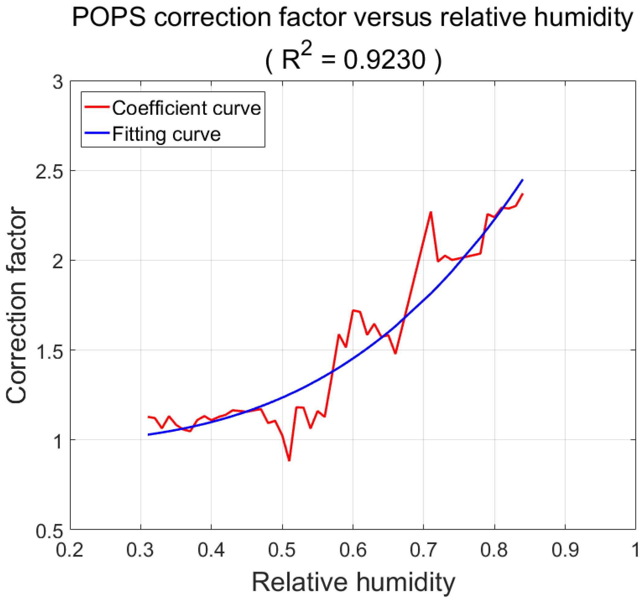
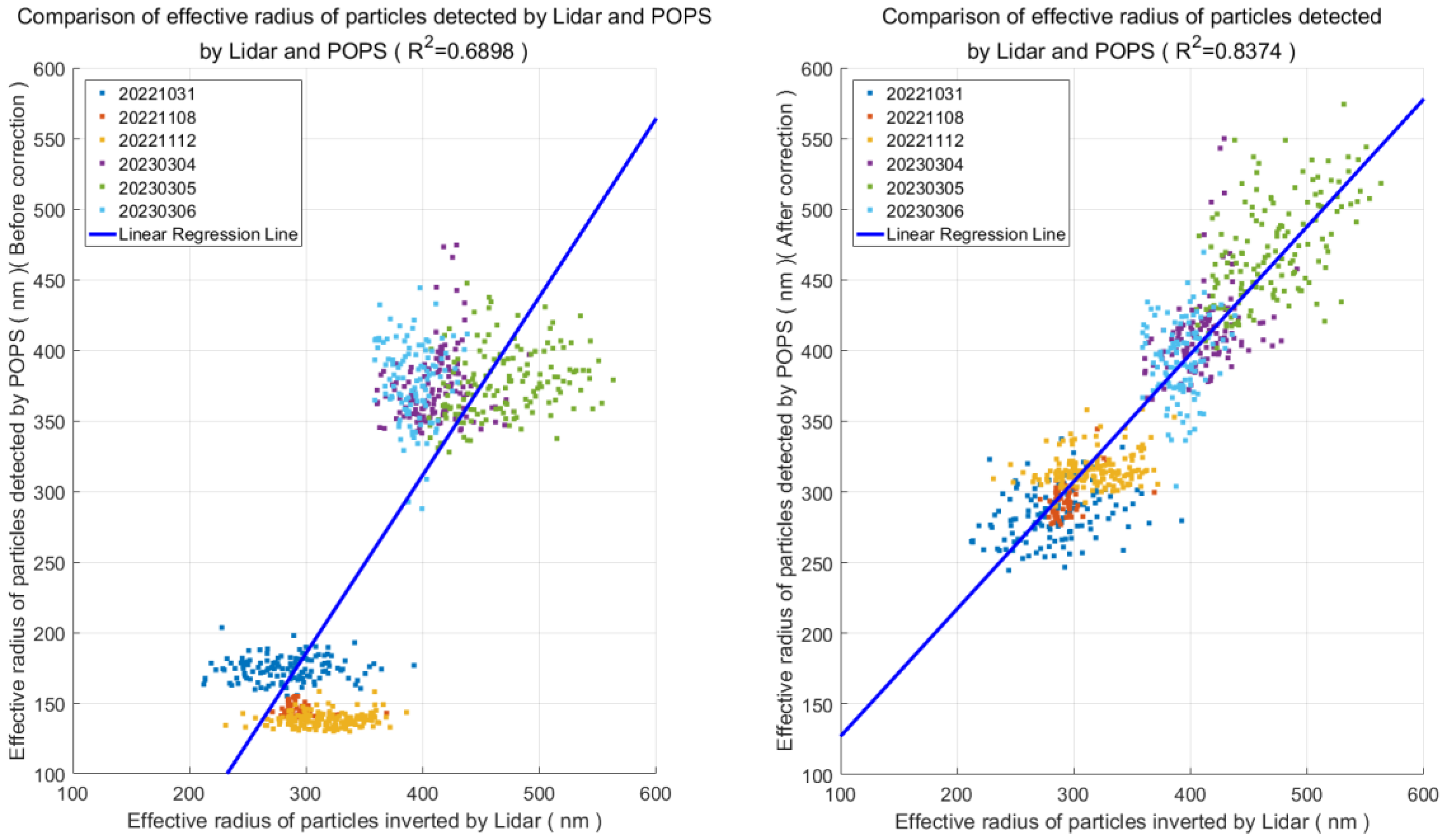
4.1. Correction of the Particle Spectrometer Detection Results

As described in Section 2.2, the aerosols detected by the particle spectrometer are drier than those retrieved by the dual-wavelength lidar, which implies that the aerosols retrieved by the lidar are considered to be wet aerosols, whereas those detected by the particle spectrometer are dry aerosols (note: “dry” refers to relative dryness compared to the ambient air). Therefore, to compare the effective particle radius detected by the particle spectrometer with the results from the dual-wavelength lidar, it is necessary to synchronize the results from both instruments under the same relative humidity conditions. This requires correcting the effective particle radius of the dry aerosols detected by the particle spectrometer, so that the corrected value corresponds to the same relative humidity as that of the wet aerosols retrieved by the dual-wavelength lidar. According to the theory of hygroscopic growth of aerosols, the ratio of the effective particle radii of wet to dry aerosols has an exponential relationship with relative humidity [12,13,14]. Thus, once this relationship is established, the results from both instruments can be synchronized to the same environmental conditions.

Four time periods of data from all three instruments were selected as sample data (hereafter referred to as “sample data”): 31 October 2022, 09:30–14:00, 8 November 2022, 22:00–23:59, 12 November 2022, 00:00–05:30, and 4 March 2023, 19:30–23:59, to analyze the ratio of the effective particle radius of wet to dry aerosols. The effective particle radius of dry aerosols detected by the particle spectrometer is known, while the effective radius of wet aerosols detected by the particle spectrometer is unknown. For this analysis, it is assumed that the effective particle radius of wet aerosols retrieved by the dual-wavelength lidar is accurate. Therefore, the effective particle radius of wet aerosols measured by the dual-wavelength lidar is used for the analysis of wet aerosols from the particle spectrometer.

At the same time, the effective particle radius retrieved by the lidar and the effective particle radius detected by the particle spectrometer for the sample data are compared by calculating the ratio between the two, and the relationship between the ratio and the corresponding relative humidity is derived. It is observed from the data in the table that the relative humidity lies within the range of [0.30, 0.90]. This table represents process data for the analysis, and due to the large volume of data, we did not display them in the manuscript. The data are classified and statistically analyzed based on relative humidity intervals, and the average ratio of effective particle radii for each interval is calculated, as shown in the bar chart of Figure 7. Meanwhile, the relative standard deviation (RSD) of all ratios within each interval was calculated to visually reflect the fluctuation of ratios across different intervals. The results are shown by the line graph in Figure 7. For example, when the ambient relative humidity (RH) falls within the range of [0.30, 0.32], the mean ratio of effective particle radii detected by the lidar and the particle spectrometer is 1.124. Within this RH range, the RSD of all ratios is 6.87%.

Analysis of Figure 7 was conducted by plotting the mean values of the ratios against relative humidity on the horizontal axis, with an exponential fitting applied as shown in Figure 8. The coefficient of determination (R²) for the fitted curve was 0.9230. This indicates that (1) a correlation exists between the effective particle radii detected by the lidar and the particle spectrometer in this study, and this correlation can be expressed by an exponential relationship; (2) the correlation is strong, with a coefficient of determination exceeding 0.92; (3) the results are consistent with the aerosol hygroscopic growth theory, providing robust scientific support. Therefore, the equation of this fitted curve can be referred to as the correction coefficient equation, expressed as follows:

$$\begin{array}{cc}y=0.98+2.64x^{3.36}& ,(x\in [0.3,0.9])\end{array}$$

(10)

where $y$ represents the correction coefficient for the effective particle radius detected by the particle spectrometer when transitioning from dry to wet aerosols and $x$ represents the atmospheric relative humidity, which ranges from [0.3, 0.9].

Thus, the correction formula for the effective particle radius detected by the particle spectrometer is as follows:

$$R_{eff}\_Corrected=R_{eff}\_Original\times y$$

(11)

where $R_{eff}\_Original$ is the effective particle radius detected by the particle spectrometer, and $R_{eff}\_Corrected$ is the corrected effective particle radius adjusted for relative humidity.

In this study, the effectiveness of the proposed correction scheme is verified using the sample data. First, the corrected results for the particle spectrometer data are obtained using the correction formulas (10) and (11). Then, the effective particle radius retrieved by the dual-wavelength lidar is compared with the corrected effective particle radius from the particle spectrometer, as shown in Figure 9. The corresponding R² values are 0.9895, 0.9896, 0.9910, and 0.9912. It can be observed that all R² values exceed 0.98, indicating that the method of using the particle spectrometer to validate the dual-wavelength lidar retrievals results is feasible. However, while the sample data validation confirms the feasibility of the method, it does not prove its universal applicability. Therefore, additional retrieval data, beyond the sample data, is required for further analysis.

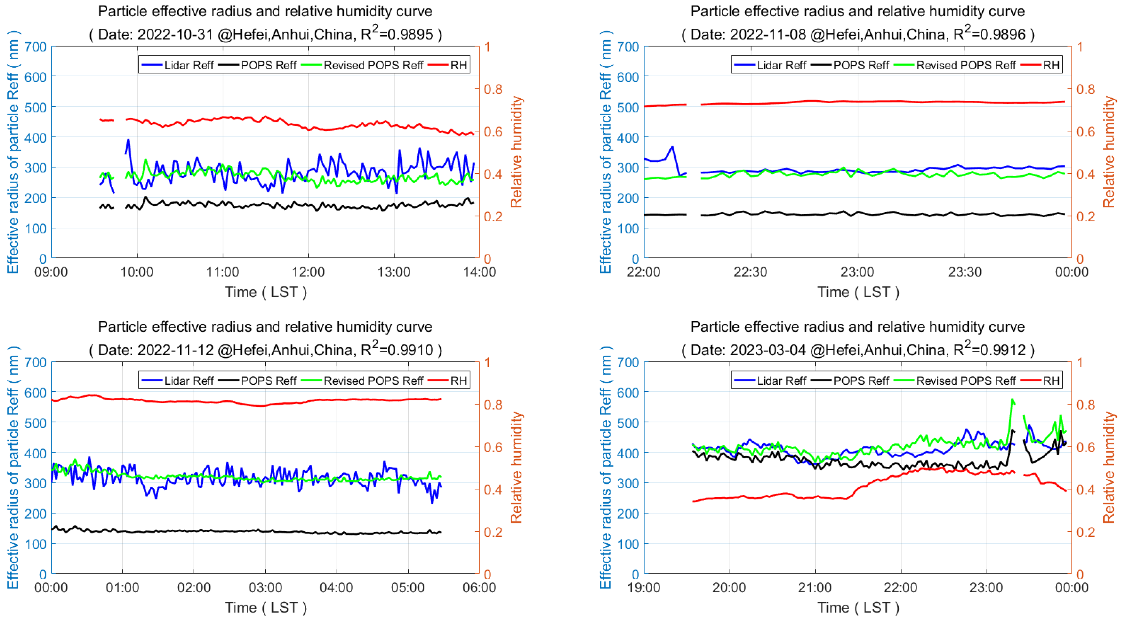
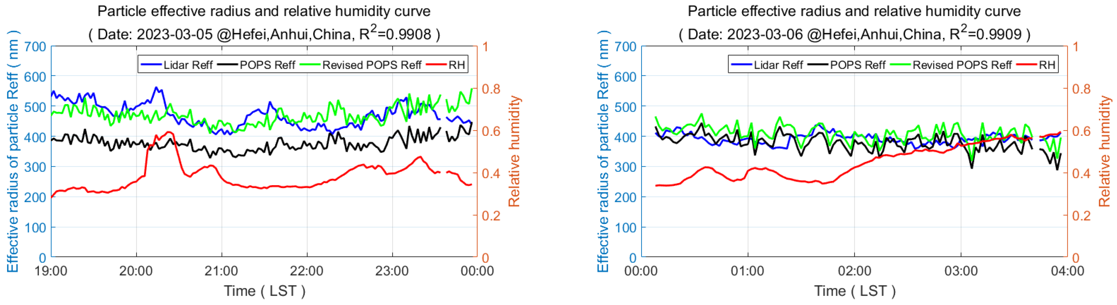
4.2. Comparison of the Dual-Wavelength Lidar and Particle Spectrometer Detection Results

To further validate the accuracy and general applicability of the dual-wavelength lidar retrieval results, retrieval data beyond the sample data were analyzed. Specifically, the particle effective radius retrieved by the dual-wavelength lidar on 5 March 2023, 19:00–23:59, and 6 March 2023, 00:00–04:00 (hereinafter referred to as the “test data”) was compared with the particle effective radius from the particle spectrometer, which was corrected for relative humidity. The correction formulas remained unchanged and continued to use Equations (10) and (11). As shown in Figure 10, the coefficient of determination (R²) between the particle effective radius corrected by the particle spectrometer and the dual-wavelength lidar results for 5 March 2023, and 6 March 2023, were 0.9908 and 0.9909, respectively, both of which were greater than 0.99. These results not only demonstrate the general applicability of the verification method proposed in this study but also confirm that the dual-wavelength lidar retrievals of aerosol particle effective radius are accurate and reliable. Furthermore, these findings support the assumption made in Section 4.1, paragraph 2.

5. Discussion

Combining both the sample and test data, Figure 11 presents the comparison of the particle effective radius retrieved by the dual-wavelength lidar with that detected by the particle spectrometer, including results before and after correction.

As can be seen from Figure 11, in the selected six months of data, the coefficient of determination (R²) between the aerosol particle effective radius detected by the two instruments was greater than 0.83, indicating a very high correlation. This shows that, under the same environmental conditions, at the same moment, the particle effective radius retrieved by the dual-wavelength lidar is strongly consistent with that detected by the particle spectrometer. This further confirms that the dual-wavelength lidar accurately reflects the actual aerosol particle effective radius in the atmosphere and also demonstrates that the lidar is operating stably, with reliable and accurate retrieval results.

6. Conclusions

This study utilizes the OPAC database and the Gamma spectrum distribution model to invert the extinction coefficient ratio of insoluble aerosols at wavelengths of 355 nm and 1064 nm. The ratio is found to exhibit a monotonically decreasing relationship with the particle effective radius in the range of [0.06, 1] μm. Based on this relationship, a lookup table was constructed for the extinction coefficient ratio and particle effective radius. Using this table, coupled with the Mie scattering lidar equation, the inversion algorithm for aerosol particle effective radius based on dual-wavelength lidar was developed. To validate the reasonableness of the inversion algorithm, a particle effective radius detection verification platform was established using an optical particle spectrometer and an automatic weather station. However, under the same detection environment, the aerosol detected by the particle spectrometer underwent some drying effects due to the internal environmental influence of the equipment, which led to discrepancies between the aerosol samples retrieved by the dual-wavelength lidar and the particle spectrometer. The particle effective radius detected by the particle spectrometer was corrected based on aerosol hygroscopic growth characteristics and the relative humidity measured by the automatic weather station. After comparing the particle effective radius retrieved by the dual-wavelength lidar and the relative humidity-corrected value from the particle spectrometer, it was found that for daily data analysis, the coefficient of determination (R²) between the results from both instruments exceeded 0.98. For data analysis over a period of six months, the coefficient of determination (R²) between the two instruments was greater than 0.83. These results confirm the stable performance of the dual-wavelength lidar system, the rationality and effectiveness of its inversion algorithm, and its strong environmental adaptability, providing a solid foundation for future all-weather atmospheric aerosol monitoring.

This study addresses the key technical challenge of rapidly inverting the aerosol particle effective radius from lidar remote sensing. The developed dual-wavelength lidar system and its inversion method enable continuous remote monitoring of aerosol microphysical properties without the need for complex calibration procedures. This advancement provides significant support for the study of aerosol morphology, haze formation and dissipation, cloud dynamics, and other microphysical processes, further strengthening the framework for meteorological forecasting, disaster prevention, and mitigation.

Future work will focus on optimizing the hardware and algorithms of the dual-wavelength lidar, further improving resolution and sensitivity to promote a more precise monitoring of aerosol particle size distribution and dynamic changes. Additionally, the system will be integrated with other atmospheric observation methods for multi-parameter monitoring, providing more comprehensive data support for regional and global climate research.

References

1. Wang, Y.J.; Hu, S.X.; Zhou, J.; Hu, H.L.; Xie, C.B.; Dong, J.H.; Yuan, K.E.; Zhang, C.Y.; Wu, X.Q.; Huang, Y.B.; et al. Lidar Atmospheric Parameter Measurement; Science Press: Beijing, China, 2014. [Google Scholar]
2. Hou, H.Y.; Liu, J.; Zhong, W.T.; Yan, K.J.; Di, H.G. Aerosol particle size distribution retrieval algorithm and error analysis based on multi-wavelength radar. In Proceedings of the Tenth International Symposium on Precision Engineering Measurements and Instrumentation, Kunming, China, 8–10 August 2018; pp. 476–481. [Google Scholar]
3. Bott, A. A numerical model of the cloud-topped planetary boundary-layer: Influence of the physico-chemical properties of aerosol particles on the effective radius of stratiform clouds. Atmos. Res. 2000, 53, 15–27. [Google Scholar] [CrossRef]
4. Wang, Y.; Lv, D.R.; Huo, J. Retrieval of cloud optical thickness and effective particle radius using transmitting solar radiation: Method study. Prog. Nat. Sci. 2006, 16, 850–858. [Google Scholar]
5. Jiang, J.H.; Su, H.; Zhai, C.; Massie, S.T.; Schoeberl, M.R.; Colarco, P.R.; Platnick, S.; Gu, Y.; Liou, K.-N. Influence of convection and aerosol pollution on ice cloud particle effective radius. Atmos. Chem. Phys. 2011, 11, 457–463. [Google Scholar] [CrossRef]
6. Chen, Q.Y.; Mao, S.; Yin, Z.P.; Yi, Y.; Li, X.; Wang, A.Z.; Wang, X. Compact and efficient 1064 nm up-conversion atmospheric lidar. Opt. Express 2023, 31, 23931–23943. [Google Scholar] [CrossRef] [PubMed]
7. Donovan, D.P.; Carswell, A.I. Principal component analysis applied to multiwavelength lidar aerosol backscatter and extinction measurements. Appl. Opt. 1997, 36, 9406–9424. [Google Scholar] [CrossRef] [PubMed]
8. Mei, F.; McMeeking, G.; Pekour, M.; Gao, R.-S.; Kulkarni, G.; China, S.; Telg, H.; Dexheimer, D.; Tomlinson, J.; Schmid, B. Performance Assessment of Portable Optical Particle Spectrometer (POPS). Sensors 2020, 20, 6294. [Google Scholar] [CrossRef] [PubMed]
9. Mei, F.; Pekour, M. Portable Optical Particle Spectrometer (POPS) Instrument Handbook; Oak Ridge National Laboratory (ORNL): Oak Ridge, TN, USA; Atmospheric Radiation Measurement (ARM) Data Center, Pacific Northwest National Lab. (PNNL): Richland, WA, USA, 2020. [Google Scholar]
10. Gao, R.S.; Telg, H.; McLaughlin, R.J.; Ciciora, S.J.; Watts, L.A.; Richardson, M.S.; Schwarz, J.P.; Perring, A.E.; Thornberry, T.D.; Rollins, A.W. A light-weight, high-sensitivity particle spectrometer for PM2.5 aerosol measurements. Aerosol Sci. Technol. 2016, 50, 88–99. [Google Scholar] [CrossRef]
11. Yu, P.F.; Rosenlof, K.H.; Liu, S.; Telg, H.; Thornberry, T.D.; Rollins, A.W.; Portmann, R.W.; Bai, Z.X.; Ray, E.A.; Duan, Y.J. Efficient transport of tropospheric aerosol into the stratosphere via the Asian summer monsoon anticyclone. Proc. Natl. Acad. Sci. USA 2017, 114, 6972–6977. [Google Scholar] [CrossRef] [PubMed]
12. Wang, L. Radiation Characteristics of Aerosol Particles/Particle System Under Different Relative Humidity. Master’s Thesis, Wuhan University of Science and Technology, Wuhan, China, 2022. [Google Scholar]
13. Xia, C. Effects of Hygroscopicity on Aerosol Optical Properties and Direct Radiative Forcing in Beijing. Ph.D. Thesis, Nanjing University of Information Science & Technology, Nanjing, China, 2023. [Google Scholar]
14. Zhang, L. Observation Study of Relative Humidity Effects on Aerosol Light Scattering at a Regional Backgound Site in the Yangtze Delta Region. Master’s Thesis, Chinese Academy of Meteorological Sciences, Beijing, China, 2014. [Google Scholar]
15. Hess, M.; Koepke, P.; Schult, I. Optical Properties of Aerosols and Clouds: The Software Package OPAC. Bull. Am. Meteorol. Soc. 1998, 79, 831–844. [Google Scholar] [CrossRef]
16. Wang, Z.X. The Precise Detection of Aerosol Particle Size Distributions of Fog/Haze the Open Atmosphere. Master’s Thesis, Xi’an University of Technology, Xi’an, China, 2019. [Google Scholar]
17. Liu, B.L. Aerosol Effective Radius Retrieval Based on Dual-Wavelength Lidar Measurement. Master’s Thesis, University of Science and Technology of China, Hefei, China, 2023. [Google Scholar]
18. Müller, D.; Wagner, F.; Wandinger, U.; Ansmann, A.; Wendisch, M.; Althausen, D.; von Hoyningen-Huene, W. Microphysical particle parameters from extinction and backscatter lidar data by inversion with regularization: Experiment. Appl. Opt. 2000, 39, 1879–1892. [Google Scholar] [CrossRef] [PubMed]
19. AboEl-Fetouh, Y.; O’Neill, N.; Ranjbar, K.; Hesaraki, S.; Abboud, I.; Sobolewski, P. Climatological-scale analysis of intensive and semi-intensive aerosol parameters derived from AERONET retrievals over the Arctic. J. Geophys. Res. Atmos. 2020, 125, e2019JD031569. [Google Scholar] [CrossRef]
20. Xiong, F.L. Study of Fitting Gamma Raindrop Size Distribution. Master’s Thesis, Nanjing University of Information Science and Technology, Nanjing, China, 2016. [Google Scholar]
21. Liu, D. Development of Polarization-Meter Lidar and Lidar Detection in the Atmospheric Boundary Layer. Ph.D. Thesis, Graduate School of the Chinese Academy of Sciences, Beijing, China, 2005. [Google Scholar]
22. Tao, Z.M.; Zhang, Y.C.; Zhang, G.X.; Lv, Y.H.; Liu, X.Q.; Tan, K.; Shao, S.S.; Hu, H.L. Properties of extinction efficiency factor of aerosol particles and fitting of scale spectrum. Chin. J. Quantum Electron. 2004, 21, 103–109. [Google Scholar]
23. Zhao, H. Atmospheric Aerosol Detection and Experimental Research Based on Multiwavelength Lidar and In-Situ Instruments. Ph.D. Thesis, Xi’an University of Technology, Xi’an, China, 2017. [Google Scholar]
24. Hansen, J.E.; Travis, L.D. Light scattering in planetary atmospheres. Space Sci. Rev. 1974, 16, 527–610. [Google Scholar] [CrossRef]
25. Mishchenko, M.I.; Travis, L.D.; Lacis, A.A. Scattering, Absorption, and Emission of Light by Small Particles; Cambridge University Press: Cambridge, UK, 2002. [Google Scholar]
26. Zhang, Z.Y.; Su, L.; Chen, L.F. Retrieval and analysis of aerosol lidar ratio at several typical regions in China. Chin. J. Lasers 2013, 40, 1–6. [Google Scholar]
Figure 1. Schematic of the dual-wavelength lidar.
Remotesensing 17 01383 g001
Figure 2. Schematic diagram of the test equipment deployment. In the figure, (A) represents the dual-wavelength lidar, which is installed on the second-floor platform, and (B) represents the support frame, which holds both an automatic weather station and a particle spectrometer at a height of approximately 3 m above the ground. The horizontal distance between (A) and (B) is 1 km.
Remotesensing 17 01383 g002
Figure 3. Top-down schematic of the portable optical particle spectrometer.
Remotesensing 17 01383 g003
Figure 4. Comparison and statistical analysis of aerosol number size distributions. The left panel illustrates a comparison between the number size distributions based on the Gamma distribution and the lognormal distribution. In this panel, the horizontal axis represents the effective particle radius, while the vertical axis indicates the number size distribution. The blue and red curves correspond to the unimodal structures of the lognormal and Gamma distributions, respectively. The right panel shows the ratio of the number of particles within different size intervals to the total number of particles in the sample. The horizontal axis represents the particle effective radius intervals with a bin width of 0.05 μm. The vertical axis indicates the proportion of data points detected in each size interval relative to the total number of particle data points in the entire sample. In other words, all particle effective radii are first obtained by the particle spectrometer; these values are then grouped by the preset size intervals, and finally, the number of data points in each interval is divided by the total number of data points in the sample to yield the ratio. This ratio is presented in two formats: a histogram (light blue) and a line graph (red). The term “POPS” in the caption of the right figure refers to the Portable Optical Particle Spectrometer.
Remotesensing 17 01383 g004
Figure 5. The relationship between particle effective radius and extinction coefficient ratio. α355 represents the extinction coefficient at 355 nm, and α1064 represents the extinction coefficient at 1064 nm. The MaxValue (0.06, 29.2) indicates that the maximum extinction coefficient ratio between the two wavelengths is 29.2, corresponding to a particle effective radius of 0.06 μm. The MinValue (1, 0.8) indicates that the minimum extinction coefficient ratio is 0.8, corresponding to a particle effective radius of 1 μm.
Remotesensing 17 01383 g005
Figure 6. Measured signals of the lidar at two wavelengths. The horizontal axis represents the horizontal range retrieved by the lidar. The effective detection range of this signal is approximately 3 km, with signals beyond this range considered as noise. (A) The blue line represents the logarithmic curve of the 355 nm channel’s echo signal after range square correction, and the red line represents the same for the 1064 nm channel. (B) The green line represents the linear fit of the 355 nm signal within its valid detection range. Half of the negative slope of this line corresponds to the extinction coefficient for the 355 nm wavelength, and the black line represents the same for the 1064 nm wavelength.
Remotesensing 17 01383 g006
Figure 7. Statistical analysis of coefficients and relative standard deviation (RSD). The horizontal axis represents the ambient relative humidity (RH) in real-time measurements. The top row of the horizontal axis indicates the RH intervals, with each interval spanning 0.02. The second row displays the average ratio of effective particle radii (left vertical axis) obtained from lidar and particle spectrometer measurements (average of ratios), presented as bar plots. The third row shows the relative standard deviation (RSD) (right vertical axis) of all effective particle radius ratios within each RH interval, depicted as a line plot. Bar plot analysis reveals that the mean ratio of effective particle radii follows an exponential trend with increasing RH. The line plot demonstrates that the RSD values remain consistently low across all RH intervals, indicating high stability in the detection results. [Note: no valid effective particle radius ratios were recorded within the RH intervals [0.66, 0.70], [0.74, 0.77], and [0.84, 0.90]. To maintain data continuity for subsequent analysis, these intervals were merged with adjacent intervals ([0.64, 0.66], [0.77, 0.78], and [0.82, 0.84], respectively).].
Remotesensing 17 01383 g007
Figure 8. Relationship between relative humidity and correction factors. The horizontal axis represents relative humidity, while the vertical axis displays the “Average of Ratios” (red line) derived from Figure 7. The blue line corresponds to the fitted curve of the “Average of Ratios”. The coefficient of determination (R2) between these two curves is indicated in the title.
Remotesensing 17 01383 g008
Figure 9. Correlation of effective particle radius from sample data. The blue line represents the effective particle radius retrieved by the dual-wavelength lidar, the black line represents the original effective particle radius detected by the particle spectrometer, the green line represents the corrected effective particle radius detected by the particle spectrometer, and the red line represents the ambient relative humidity. The R2 value in the title indicates the coefficient of determination between the effective particle radius retrieved by the lidar and the corrected effective particle radius detected by the particle spectrometer.
Remotesensing 17 01383 g009
Figure 10. Correlation of particle effective radius for test data. The blue line represents the particle effective radius retrieved by the dual-wavelength lidar, the black line represents the original particle effective radius detected by the particle spectrometer, the green line represents the particle effective radius corrected for relative humidity by the particle spectrometer, and the red line represents the environmental relative humidity. R2 in the title represents the coefficient of determination between the particle effective radius retrieved by the lidar and the particle effective radius corrected for relative humidity detected by the particle spectrometer.
Remotesensing 17 01383 g010
Figure 11. Scatter plot of retrieval results from both instruments at the same time. The horizontal axis represents the particle effective radius retrieved by the dual-wavelength lidar, the vertical axis in the left plot represents the uncorrected particle effective radius detected by the particle spectrometer, and the vertical axis in the right plot represents the corrected particle effective radius detected by the particle spectrometer. Each point corresponds to the particle effective radius at the same time. The blue line represents the linear regression line for all points, and R2 in the title represents the coefficient of determination for all scatter points. From the right plot, it is evident that the particle effective radius detected by the particle spectrometer, after correction, closely aligns with the particle effective radius retrieved by the dual-wavelength lidar, with most points concentrated around the linear regression line.
Remotesensing 17 01383 g011