

Simulation and Sensitivity Analysis of Remote Sensing Reflectance for Optically Shallow Water Bathymetry

Abstract
1. Introduction
2. Model and Methods
2.1. Parameter Selection Based on Radiative Transfer Model
2.2. Bathymetric Methods Based on Passive Optical Remote Sensing
2.3. Sensitivity Analysis Method
3. Optical Shallow Water Model Parameter Compilation
3.1. Water Depth
3.2. Water Optical Parameters
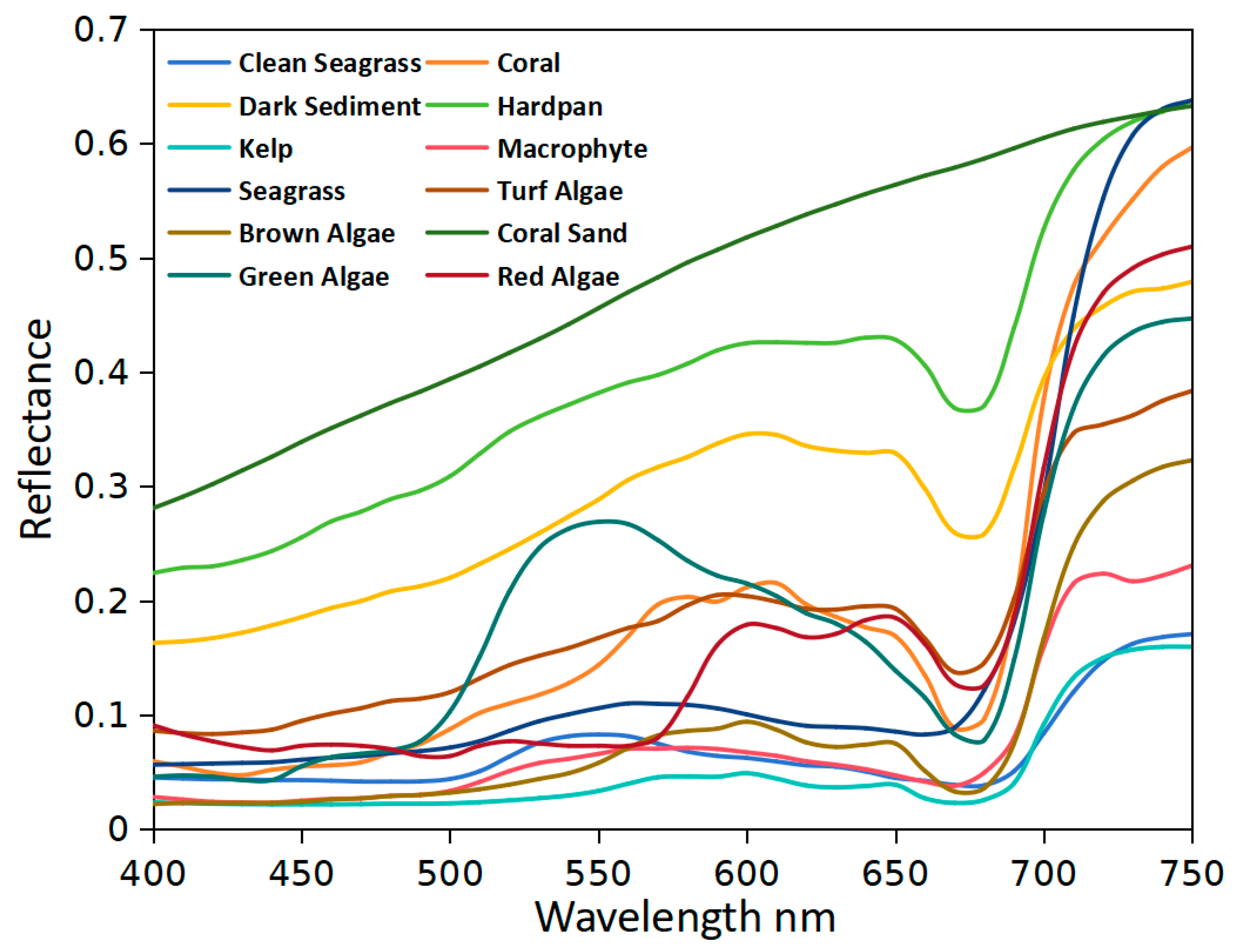
3.3. Bottom Reflectance
3.4. Noise from Above-Surface Processes
4. Results
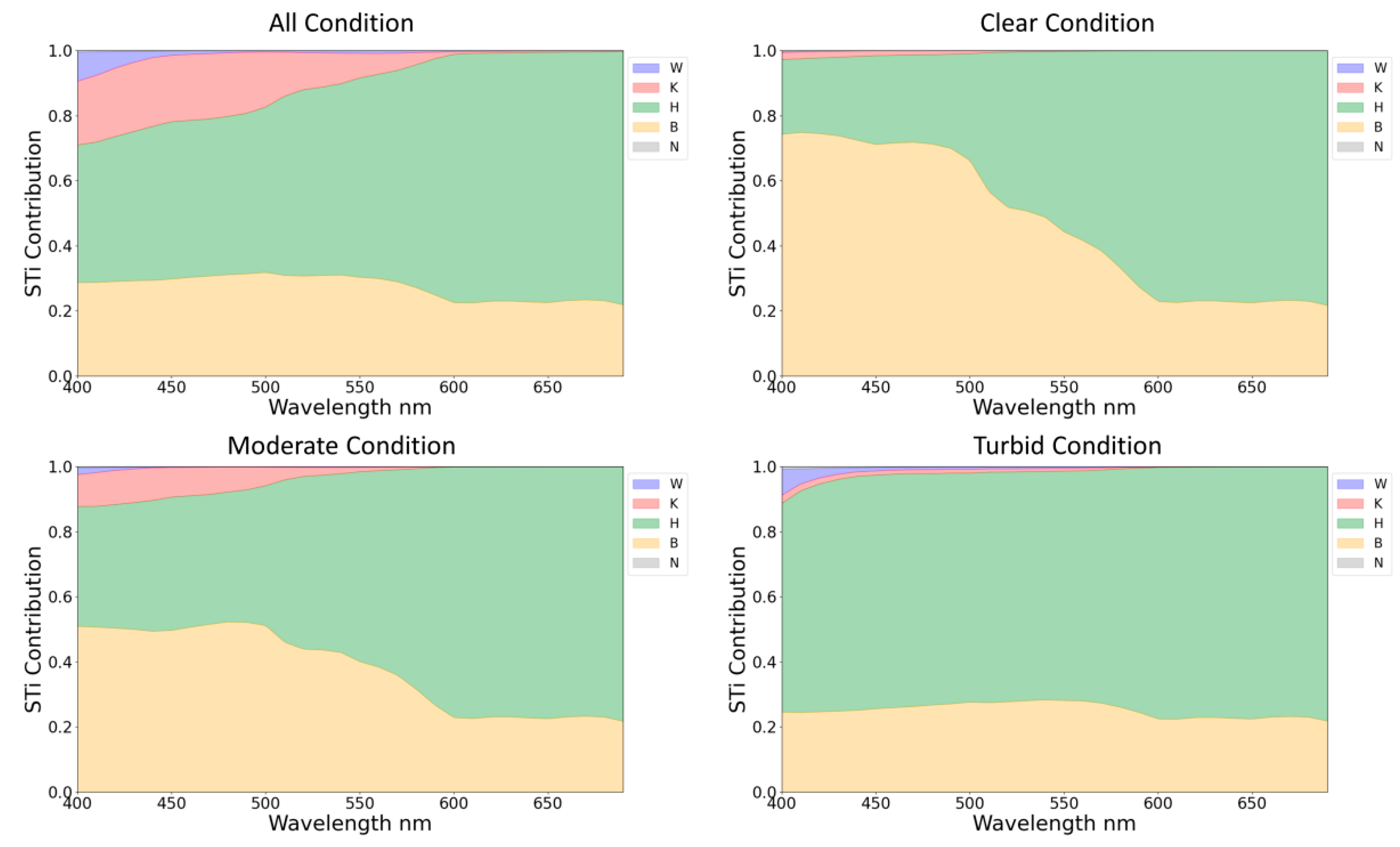
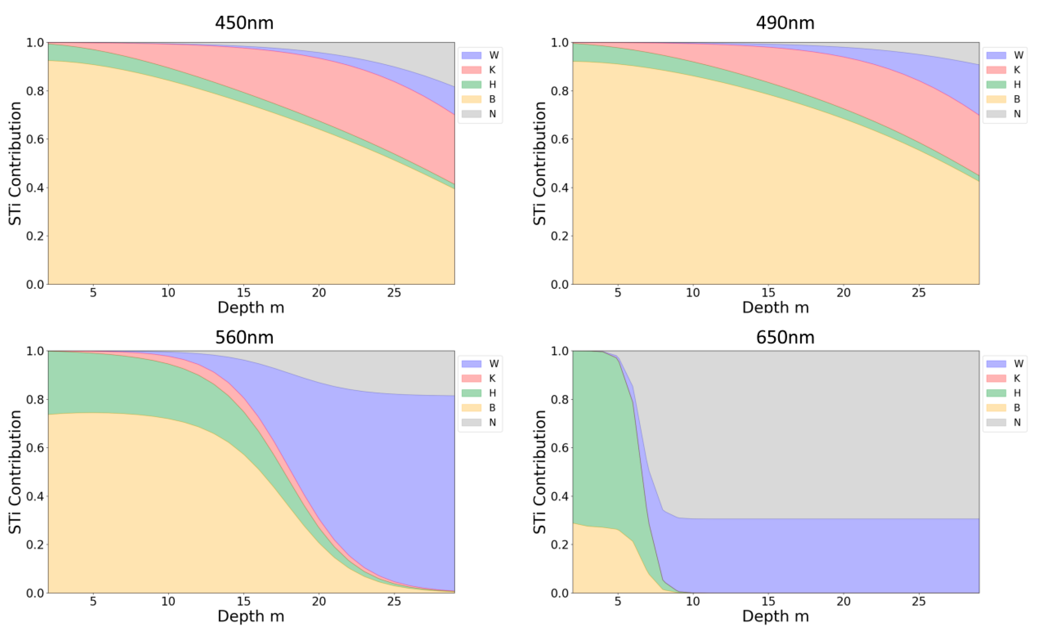
4.1. Parameter Sensitivity Across Different Parameter Ranges
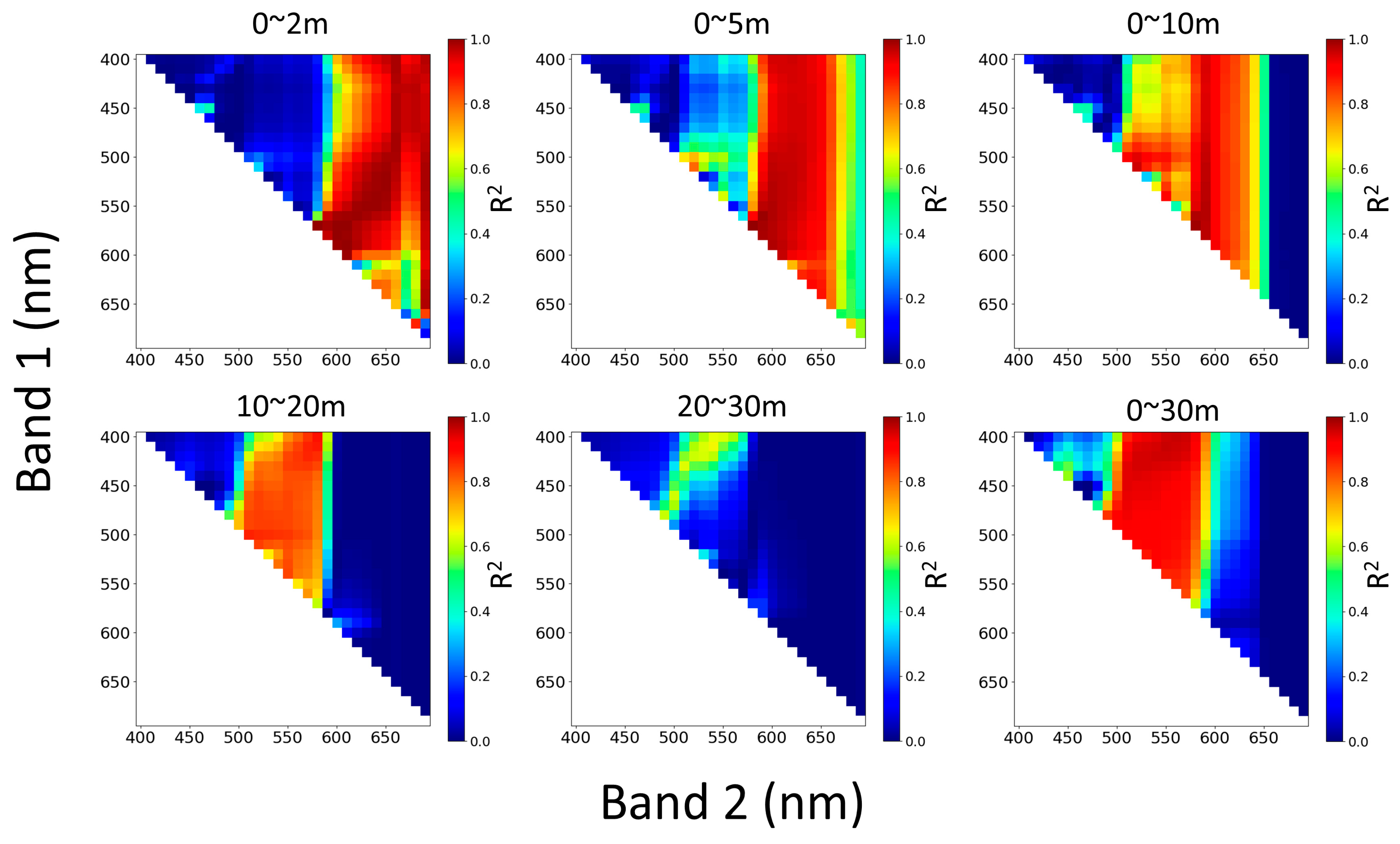
4.2. Simulation Based on the Band-Ratio Bathymetric Model
5. Discussion
6. Conclusions
Supplementary Materials
Author Contributions
Funding
Data Availability Statement
Acknowledgments
Conflicts of Interest
Appendix A

Appendix B

| Properties | Setting |
|---|---|
| IOP Specification | NEW CASE 2 IOPs |
| Pure Water IOP | Smith and Baker’s |
| Chlorophyll (Concentration) | 0.1, 0.2, 0.5, 1, 2, 5 |
| CDOM (ag(440 nm)) | 0.01, 0.1 |
| Suspend solids (Concentration) | 0.3, 3 |
| Chlorophyll-specific absorption | Medium UV absorption |
| CDOM absorption specification | Exp function; default params |
| Suspend solids scattering specification | Power law; Gordon–Morel values |
| Bioluminescence and inelastic scatter | None |
| Wavelength (nm) | 400–700; 2 nm/step |
| Sea surface wind speed (m/s) | 5 |
| Refraction index of the water | 1.34 |
| Sky model | RADTRAN-X |
| Cloud cover in percent | 0 |
| Water column | Infinitely deep |
| Solar zenith angle (°) | 45 |
References
- Kutser, T.; Hedley, J.; Giardino, C.; Roelfsema, C.; Brando, V.E. Remote sensing of shallow waters–A 50 year retrospective and future directions. Remote Sens. Environ. 2020, 240, 111169. [Google Scholar] [CrossRef]
- Fisher, R.; O’Leary, R.A.; Low-Choy, S.; Mengersen, K.; Knowlton, N.; Brainard, R.E.; Caley, M.J. Species richness on coral reefs and the pursuit of convergent global estimates. Curr. Biol. 2015, 25, 500–505. [Google Scholar] [CrossRef] [PubMed]
- Stumpf, R.P.; Holderied, K.; Sinclair, M. Determination of water depth with high-resolution satellite imagery over variable bottom types. Limnol. Oceanogr. 2003, 48, 547–556. [Google Scholar] [CrossRef]
- Lyzenga, D.R. Passive Remote-Sensing Techniques for Mapping Water Depth and Bottom Features. Appl. Opt. 1978, 17, 379–383. [Google Scholar] [CrossRef] [PubMed]
- Lee, Z.; Carder, K.L.; Mobley, C.D.; Steward, R.G.; Patch, J.S. Hyperspectral remote sensing for shallow waters: 2 Deriving bottom depths and water properties by optimization. Appl. Opt. 1999, 38, 3831–3843. [Google Scholar] [CrossRef]
- Lee, Z.P.; Carder, K.L.; Arnone, R.A. Deriving inherent optical properties from water color: A multiband quasi-analytical algorithm for optically deep waters. Appl. Opt. 2002, 41, 5755–5772. [Google Scholar] [CrossRef]
- Xia, H.; Li, X.; Zhang, H.; Wang, J.; Lou, X.; Fan, K.; Shi, A.; Li, D. A Bathymetry Mapping Approach Combining Log-Ratio and Semianalytical Models Using Four-Band Multispectral Imagery Without Ground Data. IEEE Trans. Geosci. Remote Sens. 2020, 58, 2695–2709. [Google Scholar] [CrossRef]
- Thompson, D.R.; Hochberg, E.J.; Asner, G.P.; Green, R.O.; Knapp, D.E.; Gao, B.-C.; Garcia, R.; Gierach, M.; Lee, Z.; Maritorena, S.; et al. Airborne mapping of benthic reflectance spectra with Bayesian linear mixtures. Remote Sens. Environ. 2017, 200, 18–30. [Google Scholar] [CrossRef]
- Iwanaga, T.; Usher, W.; Herman, J. Toward SALib 2.0: Advancing the accessibility and interpretability of global sensitivity analyses. Socio Environ. Syst. Model. 2022, 4, 18155. [Google Scholar] [CrossRef]
- Verrelst, J.; Rivera, J.P.; van der Tol, C.; Magnani, F.; Mohammed, G.; Moreno, J. Global sensitivity analysis of the SCOPE model: What drives simulated canopy-leaving sun-induced fluorescence? Remote Sens. Environ. 2015, 166, 8–21. [Google Scholar] [CrossRef]
- Zhou, G.; Ma, Z.; Sathyendranath, S.; Platt, T.; Jiang, C.; Sun, K. Canopy Reflectance Modeling of Aquatic Vegetation for Algorithm Development: Global Sensitivity Analysis. Remote Sens. 2018, 10, 837. [Google Scholar] [CrossRef]
- He, J.; Zhang, S.; Cui, X.; Feng, W. Remote sensing for shallow bathymetry: A systematic review. Earth Sci. Rev. 2024, 258, 104957. [Google Scholar] [CrossRef]
- Qi, J.; Zhang, D.; Ren, Z.; Cui, A.; Yin, F.; Qin, J.; Zhan, J.; Zhu, J. Determination of the Initial Value Ranges of Nonlinear Solutions for a Log Ratio Bathymetric Inversion Model and Bathymetry Retrieval. IEEE J. Sel. Top. Appl. Earth Obs. Remote Sens. 2021, 14, 10875–10888. [Google Scholar] [CrossRef]
- Li, J.; Knapp, D.E.; Schill, S.R.; Roelfsema, C.; Phinn, S.; Silman, M.; Mascaro, J.; Asner, G.P. Adaptive bathymetry estimation for shallow coastal waters using Planet Dove satellites. Remote Sens. Environ. 2019, 232, 111302. [Google Scholar] [CrossRef]
- Yang, Q.; Chen, J.; Chen, B.; Tao, B. Evaluation and Improvement of No-Ground-Truth Dual Band Algorithm for Shallow Water Depth Retrieval: A Case Study of a Coastal Island. Remote Sens. 2022, 14, 6231. [Google Scholar] [CrossRef]
- Gwon, Y.; Kwon, S.; Kim, D.; Seo, I.W.; You, H. Estimation of shallow stream bathymetry under varying suspended sediment concentrations and compositions using hyperspectral imagery. Geomorphology 2023, 433, 108772. [Google Scholar] [CrossRef]
- Kim, J.S.; Baek, D.; Seo, I.W.; Shin, J. Retrieving shallow stream bathymetry from UAV-assisted RGB imagery using a geospatial regression method. Geomorphology 2019, 341, 102–114. [Google Scholar] [CrossRef]
- Barnes, B.B.; Hu, C.; Schaeffer, B.A.; Lee, Z.; Palandro, D.A.; Lehrter, J.C. MODIS-derived spatiotemporal water clarity patterns in optically shallow Florida Keys waters: A new approach to remove bottom contamination. Remote Sens. Environ. 2013, 134, 377–391. [Google Scholar] [CrossRef]
- Barnes, B.B.; Garcia, R.; Hu, C.; Lee, Z. Multi-band spectral matching inversion algorithm to derive water column properties in optically shallow waters: An optimization of parameterization. Remote Sens. Environ. 2018, 204, 424–438. [Google Scholar] [CrossRef]
- Douglas-Smith, D.; Iwanaga, T.; Croke, B.F.W.; Jakeman, A.J. Certain trends in uncertainty and sensitivity analysis: An overview of software tools and techniques. Environ. Model. Softw. 2020, 124, 104588. [Google Scholar] [CrossRef]
- Ferretti, F.; Saltelli, A.; Tarantola, S. Trends in sensitivity analysis practice in the last decade. Sci. Total Environ. 2016, 568, 666–670. [Google Scholar] [CrossRef] [PubMed]
- Saltelli, A.; Aleksankina, K.; Becker, W.; Fennell, P.; Ferretti, F.; Holst, N.; Li, S.; Wu, Q. Why so many published sensitivity analyses are false: A systematic review of sensitivity analysis practices. Environ. Model. Softw. 2019, 114, 29–39. [Google Scholar] [CrossRef]
- Sobol, I.M. Global sensitivity indices for nonlinear mathematical models and their Monte Carlo estimates. Math. Comput. Simulat. 2001, 55, 271–280. [Google Scholar] [CrossRef]
- Reed, P.M.; Hadjimichael, A.; Malek, K.; Karimi, T.; Vernon, C.R.; Srikrishnan, V.; Gupta, R.S.; Gold, D.F.; Lee, B.; Keller, K.; et al. Addressing Uncertainty in MultiSector Dynamics Research; Pacific Northwest National Laboratory (PNNL): Richland, WA, USA, 2022. [Google Scholar]
- Saltelli, A.; Annoni, P.; Azzini, I.; Campolongo, F.; Ratto, M.; Tarantola, S. Variance based sensitivity analysis of model output. Design and estimator for the total sensitivity index. Comput. Phys. Commun. 2010, 181, 259–270. [Google Scholar] [CrossRef]
- Kerr, J.M.; Purkis, S. An algorithm for optically-deriving water depth from multispectral imagery in coral reef landscapes in the absence of ground-truth data. Remote Sens. Environ. 2018, 210, 307–324. [Google Scholar] [CrossRef]
- Chen, B.; Yang, Y.; Xu, D.; Huang, E. A dual band algorithm for shallow water depth retrieval from high spatial resolution imagery with no ground truth. ISPRS J. Photogramm. Remote Sens. 2019, 151, 1–13. [Google Scholar] [CrossRef]
- Wei, J.; Wang, M.; Lee, Z.; Briceño, H.O.; Yu, X.; Jiang, L.; Garcia, R.; Wang, J.; Luis, K. Shallow water bathymetry with multi-spectral satellite ocean color sensors: Leveraging temporal variation in image data. Remote Sens. Environ. 2020, 250, 112035. [Google Scholar] [CrossRef]
- Surisetty, V.V.A.K.; Venkateswarlu, C.; Gireesh, B.; Prasad, K.V.S.R.; Sharma, R. On improved nearshore bathymetry estimates from satellites using ensemble and machine learning approaches. Adv. Space Res. 2021, 68, 3342–3364. [Google Scholar] [CrossRef]
- Wu, Z.; Mao, Z.; Shen, W. Integrating Multiple Datasets and Machine Learning Algorithms for Satellite-Based Bathymetry in Seaports. Remote Sens. 2021, 13, 4328. [Google Scholar] [CrossRef]
- He, J.; Lin, J.; Ma, M.; Liao, X. Mapping topo-bathymetry of transparent tufa lakes using UAV-based photogrammetry and RGB imagery. Geomorphology 2021, 389, 107832. [Google Scholar] [CrossRef]
- Lee, J.-S.; Baek, J.-Y.; Jung, D.; Shim, J.-S.; Lim, H.-S.; Jo, Y.-H. Estimate of Coastal Water Depth Based on Aerial Photographs Using a Low-Altitude Remote Sensing System. Ocean. Sci. J. 2019, 54, 349–362. [Google Scholar] [CrossRef]
- Kasvi, E.; Salmela, J.; Lotsari, E.; Kumpula, T.; Lane, S.N. Comparison of remote sensing based approaches for mapping bathymetry of shallow, clear water rivers. Geomorphology 2019, 333, 180–197. [Google Scholar] [CrossRef]
- Legleiter, C.J.; Stegman, T.K.; Overstreet, B.T. Spectrally based mapping of riverbed composition. Geomorphology 2016, 264, 61–79. [Google Scholar] [CrossRef]
- Woodget, A.S.; Dietrich, J.T.; Wilson, R.T. Quantifying Below-Water Fluvial Geomorphic Change: The Implications of Refraction Correction, Water Surface Elevations, and Spatially Variable Error. Remote Sens. 2019, 11, 2415. [Google Scholar] [CrossRef]
- Zhou, W.; Tang, Y.; Jing, W.; Li, Y.; Yang, J.; Deng, Y.; Zhang, Y. A Comparison of Machine Learning and Empirical Approaches for Deriving Bathymetry from Multispectral Imagery. Remote Sens. 2023, 15, 393. [Google Scholar] [CrossRef]
- Lee, Z.; Shang, S.; Hu, C.; Du, K.; Weidemann, A.; Hou, W.; Lin, J.; Lin, G. Secchi disk depth: A new theory and mechanistic model for underwater visibility. Remote Sens. Environ. 2015, 169, 139–149. [Google Scholar] [CrossRef]
- Gimond, M. Description and verification of an aquatic optics Monte Carlo model. Environ. Model. Softw. 2004, 19, 1065–1076. [Google Scholar] [CrossRef]
- Liu, Y.; Tang, D.; Deng, R.; Cao, B.; Chen, Q.; Zhang, R.; Qin, Y.; Zhang, S. An Adaptive Blended Algorithm Approach for Deriving Bathymetry from Multispectral Imagery. IEEE J. Sel. Top. Appl. Earth Obs. Remote Sens. 2021, 14, 801–817. [Google Scholar] [CrossRef]
- Li, J.; Yu, Q.; Tian, Y.Q.; Becker, B.L. Remote sensing estimation of colored dissolved organic matter (CDOM) in optically shallow waters. ISPRS J. Photogramm. Remote Sens. 2017, 128, 98–110. [Google Scholar] [CrossRef]
- Matsushita, B.; Yang, W.; Chang, P.; Yang, F.; Fukushima, T. A simple method for distinguishing global Case-1 and Case-2 waters using SeaWiFS measurements. ISPRS J. Photogramm. Remote Sens. 2012, 69, 74–87. [Google Scholar] [CrossRef]
- Morel, A.; Prieur, L. Analysis of Variations in Ocean Color. Limnol. Oceanogr. 1977, 22, 709–722. [Google Scholar] [CrossRef]
- Service, C.M. Global Ocean Colour (Copernicus-GlobColour), Bio-Geo-Chemical, L3 (Daily) from Satellite Observations (1997-ongoing). 2024. Available online: https://data.marine.copernicus.eu/product/OCEANCOLOUR_GLO_BGC_L3_MY_009_103/description (accessed on 28 February 2025).
- Wei, J.W.; Lee, Z.P.; Shang, S.L. A system to measure the data quality of spectral remote-sensing reflectance of aquatic environments. J. Geophys. Res. Ocean. 2016, 121, 8189–8207. [Google Scholar] [CrossRef]
- Wei, J.W.; Lee, Z.; Shang, S.L.; Yu, X.L. Semianalytical Derivation of Phytoplankton, CDOM, and Detritus Absorption Coefficients From the Landsat 8/OLI Reflectance in Coastal Waters. J. Geophys. Res. Ocean. 2019, 124, 3682–3699. [Google Scholar] [CrossRef]
- Wei, J.W.; Yu, X.L.; Lee, Z.P.; Wang, M.H.; Jiang, L.D. Improving low-quality satellite remote sensing reflectance at blue bands over coastal and inland waters. Remote Sens. Environ. 2020, 250, 112029. [Google Scholar] [CrossRef]
- Yan, N.Y.; Sun, Z.; Huang, W.; Jun, Z.; Sun, S.J. Assessing Landsat-8 atmospheric correction schemes in low to moderate turbidity waters from a global perspective. Int. J. Digit. Earth 2023, 16, 66–92. [Google Scholar] [CrossRef]
- Jeba Dev, P.; Anna Geevarghese, G.; Purvaja, R.; Ramesh, R. Measurement of in-vivo spectral reflectance of bottom types: Implications for remote sensing of shallow waters. Adv. Space Res. 2022, 69, 4240–4251. [Google Scholar] [CrossRef]
- Hochberg, E. Spectral reflectance of coral reef bottom-types worldwide and implications for coral reef remote sensing. Remote Sens. Environ. 2003, 85, 159–173. [Google Scholar] [CrossRef]
- Gege, P.; Dekker, A.G. Spectral and Radiometric Measurement Requirements for Inland, Coastal and Reef Waters. Remote Sens. 2020, 12, 2247. [Google Scholar] [CrossRef]
- Xu, J.; Zhao, J.; Wang, F.; Chen, Y.; Lee, Z. Detection of Coral Reef Bleaching Based on Sentinel-2 Multi-Temporal Imagery: Simulation and Case Study. Front. Mar. Sci. 2021, 8, 584263. [Google Scholar] [CrossRef]
- Zoffoli, M.L.; Gernez, P.; Rosa, P.; Le Bris, A.; Brando, V.E.; Barillé, A.-L.; Harin, N.; Peters, S.; Poser, K.; Spaias, L.; et al. Sentinel-2 remote sensing of Zostera noltei-dominated intertidal seagrass meadows. Remote Sens. Environ. 2020, 251, 112020. [Google Scholar] [CrossRef]
- Melin, F.; Zibordi, G.; Berthon, J.-F. Uncertainties in Remote Sensing Reflectance From MODIS-Terra. IEEE Geosci. Remote Sens. Lett. 2012, 9, 432–436. [Google Scholar] [CrossRef]
- Mélin, F.; Sclep, G.; Jackson, T.; Sathyendranath, S. Uncertainty estimates of remote sensing reflectance derived from comparison of ocean color satellite data sets. Remote Sens. Environ. 2016, 177, 107–124. [Google Scholar] [CrossRef]
- Gilerson, A.; Herrera-Estrella, E.; Foster, R.; Agagliate, J.; Hu, C.; Ibrahim, A.; Franz, B. Determining the Primary Sources of Uncertainty in Retrieval of Marine Remote Sensing Reflectance From Satellite Ocean Color Sensors. Front. Remote Sens. 2022, 3, 857530. [Google Scholar] [CrossRef]
- Gilerson, A.; Herrera-Estrella, E.; Agagliate, J.; Foster, R.; Gossn, J.I.; Dessailly, D.; Kwiatkowska, E. Determining the primary sources of uncertainty in the retrieval of marine remote sensing reflectance from satellite ocean color sensors II. Sentinel 3 OLCI sensors. Front. Remote Sens. 2023, 4, 1146110. [Google Scholar] [CrossRef]
- Wirasatriya, A.; Maslukah, L.; Indrayanti, E.; Yusuf, M.; Milenia, A.P.; Adam, A.A.; Helmi, M. Seasonal variability of Total Suspended Sediment off the Banjir Kanal Barat River, Semarang, Indonesia estimated from Sentinel-2 images. Reg. Stud. Mar. Sci. 2023, 57, 102735. [Google Scholar] [CrossRef]
- Jiang, D.L.; Matsushita, B.; Pahlevan, N.; Gurlin, D.; Fichot, G.G.; Harringmeyer, J.; Sent, G.; Brito, A.C.; Brotas, V.; Werther, M.; et al. Estimating the concentration of total suspended solids in inland and coastal waters from Sentinel-2 MSI: A semi-analytical approach. Isprs J. Photogramm. Remote Sens. 2023, 204, 362–377. [Google Scholar] [CrossRef]
- Dogliotti, A.I.; Ruddick, K.G.; Nechad, B.; Doxaran, D.; Knaeps, E. A single algorithm to retrieve turbidity from remotely-sensed data in all coastal and estuarine waters. Remote Sens. Environ. 2015, 156, 157–168. [Google Scholar] [CrossRef]


| Component | Unit | Class |
|---|---|---|
| Chlorophyll (concentration) | mg/m3 | 0.1, 0.2, 0.5, 1, 2, 5 |
| CDOM (ag(440 nm)) | m−1 | 0.01, 0.1 |
| Suspended solids (concentration) | g/m3 | 0.3, 3 |
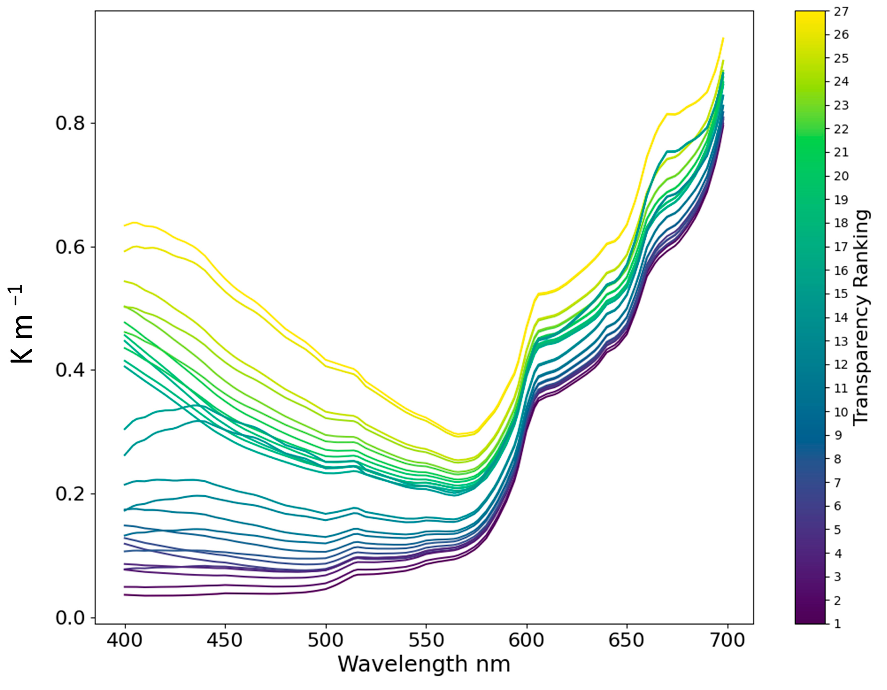
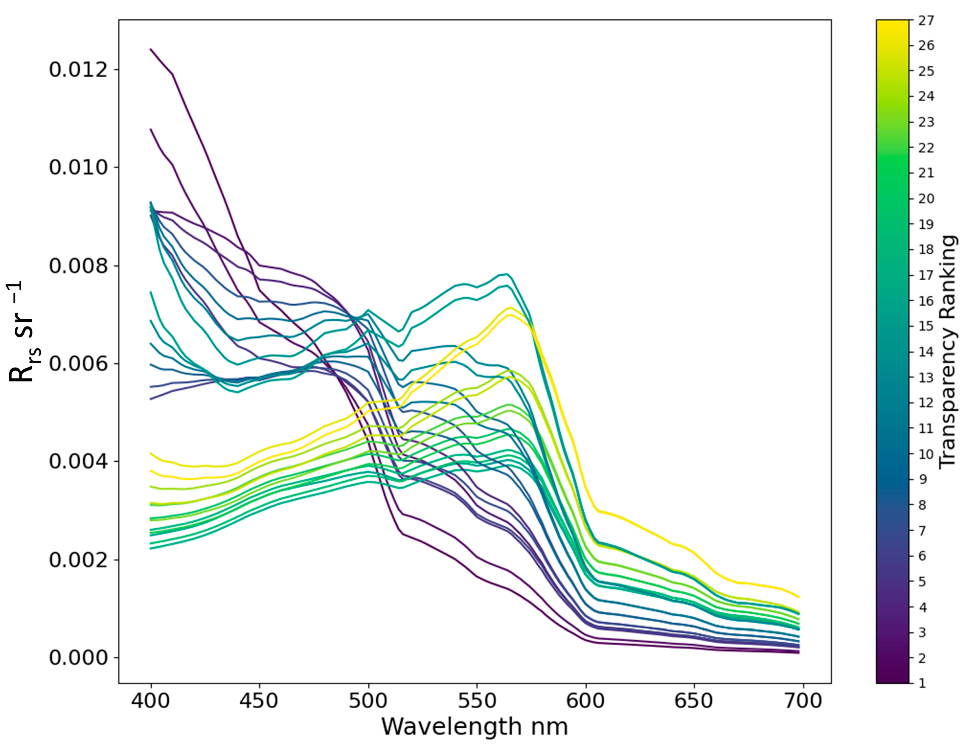
| Condition | AOP Range | Bottom Type |
|---|---|---|
| Clear | Ranking 1~3 in Figure 3 and Figure 4 | From Kelp to Sand in Figure 5 |
| Moderate | Ranking 1~12 in Figure 3 and Figure 4 | From Kelp to Sand in Figure 5 |
| Turbid | Ranking 13~27 in Figure 3 and Figure 4 | From Kelp to Sand in Figure 5 |
Disclaimer/Publisher’s Note: The statements, opinions and data contained in all publications are solely those of the individual author(s) and contributor(s) and not of MDPI and/or the editor(s). MDPI and/or the editor(s) disclaim responsibility for any injury to people or property resulting from any ideas, methods, instructions or products referred to in the content. |
© 2025 by the authors. Licensee MDPI, Basel, Switzerland. This article is an open access article distributed under the terms and conditions of the Creative Commons Attribution (CC BY) license (https://creativecommons.org/licenses/by/4.0/).
Share and Cite
Wang, E.; Zhang, H.; Wang, J.; Cao, W.; Li, D. Simulation and Sensitivity Analysis of Remote Sensing Reflectance for Optically Shallow Water Bathymetry. Remote Sens. 2025, 17, 1384. https://doi.org/10.3390/rs17081384
Wang E, Zhang H, Wang J, Cao W, Li D. Simulation and Sensitivity Analysis of Remote Sensing Reflectance for Optically Shallow Water Bathymetry. Remote Sensing. 2025; 17(8):1384. https://doi.org/10.3390/rs17081384
Chicago/Turabian StyleWang, Enze, Huaguo Zhang, Juan Wang, Wenting Cao, and Dongling Li. 2025. "Simulation and Sensitivity Analysis of Remote Sensing Reflectance for Optically Shallow Water Bathymetry" Remote Sensing 17, no. 8: 1384. https://doi.org/10.3390/rs17081384
APA StyleWang, E., Zhang, H., Wang, J., Cao, W., & Li, D. (2025). Simulation and Sensitivity Analysis of Remote Sensing Reflectance for Optically Shallow Water Bathymetry. Remote Sensing, 17(8), 1384. https://doi.org/10.3390/rs17081384