Abstract
Coordinate registration (CR) is the key technology for improving the target positioning accuracy of sky-wave over-the-horizon radar (OTHR). The CR parameters are derived by matching the sea–land clutter classification (SLCC) results with prior geographic information. However, the SLCC results often contain mixed clutter, leading to discrepancies between land and island contours and prior geographic information, which makes it challenging to calculate accurate CR parameters for OTHR. To address these challenges, we transform the sea–land clutter data from Euclidean space into graph data in non-Euclidean space, and the CR parameters are obtained by calculating the similarity between graph pairs. And then, we propose a similarity calculation via a graph neural network (SC-GNN) method for calculating the similarity between graph pairs, which involves subgraph-level interactions and node-level comparisons. By partitioning the graph into subgraphs, SC-GNN effectively captures the local features within the SLCC results, enhancing the model’s flexibility and improving its performance. For validation, we construct three datasets: an original sea–land clutter dataset, a sea–land clutter cluster dataset, and a sea–land clutter registration dataset, with the samples drawn from various seasons, times, and detection areas. Compared with the existing graph matching methods, the proposed SC-GNN achieves a Spearman’s rank correlation coefficient of at least 0.800, a Kendall’s rank correlation coefficient of at least 0.639, a p@10 of at least 0.706, and a p@20 of at least 0.845.
1. Introduction
Sky-wave over-the-horizon radar (OTHR) is a crucial sensing technology in remote sensing due to its long-range detection capability [1,2]. Sea–land clutter classification (SLCC) is the key technology for enhancing the target positioning accuracy of OTHR. By matching the SLCC results with an electronic map, the coordinate registration (CR) parameters for OTHR are derived, demonstrating significant potential to improve the target positioning accuracy in a cost-effective manner [3,4,5].
In recent years, there have been considerable works on SLCC, including model-driven and data-driven methods. In terms of the model-driven SLCC methods, Turley et al. [6] converted sea–land clutter data into graph data and constructed a graph edge equation based on adjacent azimuth–range cells. The SLCC task was realized by solving the equation using the weighted least square method. Jin et al. [7] proposed an SLCC method based on a support vector machine by analyzing three kinds of features of the sea–land clutter data. In [6,7], designing a feature extractor to convert sea–land clutter data into a suitable feature vector required both careful engineering and substantial domain expertise. This transformation enables the classifier to categorize the data into distinct classes. Although the model-driven-based SLCC methods in [6,7] can achieve SLCC, their effectiveness may be constrained by the complex nature of both the ionosphere and sea–land clutter. As noted in [8], identifying an appropriate model for fitting sea–land clutter is often challenging. Moreover, the features of sea–land clutter are difficult to extract manually and exhibit instability. With the wide application of deep learning in radar image processing [9,10,11], many SLCC methods based on deep convolutional neural networks (DCNNs) have been proposed. Li et al. [8] proposed a method that utilized a DCNN to classify sea–land clutter by automatically extracting the high-dimensional hidden features from massive sea–land clutter data. Specifically, a DCNN with three convolutional layers and two fully connected layers was employed for classification. Li et al. [12] proposed a cross-resolution classification method based on the algebraic relationship between sea–land clutter data at different resolutions. By modifying the weight of the residual neural networks, the performance of the SLCC model was improved. Li et al. [13] proposed an attention-aided pyramid scene parsing network that effectively integrated contextual and global information from the range–Doppler (RD) map. This method could fuse multi-scale information and facilitate more stable model training, thereby significantly improving both the performance and robustness of the SLCC model. Jiang et al. [14] proposed a deep embedded convolutional clustering method that employed a convolutional auto-encoder to reconstruct sea–land clutter data. This method subsequently applied clustering loss to class the unlabeled samples, thereby achieve the SLCC task. Zhang et al. [15] introduced a method for augmenting and classifying sea–land clutter data utilizing an auxiliary classifier, a variational autoencoder, and generative adversarial networks. This method enabled the extraction of latent features from limited labeled samples, thereby achieving high-quality sample synthesis and accurate classification. Zhang et al. [16] proposed an SLCC method utilizing triple loss adversarial domain adaptation networks to address cross-domain classification challenges. By learning domain-invariant features across the feature, instance, and class levels, this method significantly improved the performance of the SLCC model in cross-domain settings. Zhang et al. [17] proposed a weighted loss semi-supervised generative adversarial network that significantly enhanced the performance of a fully supervised SLCC model. This improvement was achieved by effectively utilizing a limited set of labeled samples in conjunction with a large corpus of unlabeled sea–land clutter data. Although several efficient and effective data-driven SLCC methods have been proposed in in [8,12,13,14,15,16,17], they have not explored SLCC-based CR methods for OTHR. Therefore, it is necessary to study CR methods for OTHR based on SLCC further.
A SLCC-based CR method has the following difficulties. Firstly, there are oceans, lands, and islands in the OTHR detection area. Therefore, there is sea clutter, land clutter, and mixed clutter in the RD map. Mixed clutter contains the characteristics of both sea clutter and land clutter, which are difficult to subdivide further into sea clutter or land clutter, resulting in nonlinear differences between the SLCC results and the electronic map. Secondly, searching for the results that are most similar to the SLCC results from the electronic map requires a lot of computation due to the complex spatial relations.
By matching the SLCC results with the electronic map, the CR parameters can be obtained by calculating the similarity between images. Image matching is a fundamental problem in computer science which aims to identify and match similar or corresponding regions between images. With the rapid development of graph neural networks (GNNs), they have achieved remarkable success in a wide range of graph-based machine learning tasks, such as node classification [18], link prediction [19], graph classification [20], and graph generation [21]. However, there has been less study on learning the similarity scores between two graphs using GNNs. Compared with the traditional similarity calculation methods, the main advantage of a GNN in image similarity calculations is that it can capture the structure information of the image and deal with the complex spatial relations better. After converting the SLCC results and the electronic map into graph data, the CR parameters can be calculated through graph similarity calculations.
To this end, we propose a framework for calculating the CR parameters, including graph construction, mixed clutter clustering, and graph similarity calculations. Specifically, in the graph construction, the correlation of adjacent azimuth–range cells in the sea–land clutter data is analyzed from three aspects: the difference in the signal energy difference, the difference in the signal direction, and the signal correlation. In the mixed clutter clustering, to acquire more accurate land or island information, we subdivide the mixed clutter in the SLCC results further into sea clutter or land clutter based on the prior geographic information and the nearest neighbor idea. And then, we obtain the CR parameters by calculating the similarity between graph pairs and propose the method of similarity calculation via a graph neural network (SC-GNN) for calculating the similarity. In SC-GNN, the graphs are segmented into subgraphs to capture the local features in the SLCC results better. Then, subgraph pairs with higher similarity scores are compared at the node level.
In summary, the main contributions of this article cover the following aspects:
(1) A framework for calculating CR parameters in OTHR is proposed. The calculation of the CR parameters is transformed into a graph similarity calculation problem.
(2) By analyzing the correlation between adjacent azimuth–range cells in the sea–land clutter data, a graph construction method for converting sea–land clutter data from Euclidean space into graph data in non-Euclidean space is proposed.
(3) The proposed KNN-MCC can effectively subdivide the mixed clutter into sea clutter or land clutter to obtain more accurate land and island information in the detection area.
(4) The proposed SC-GNN is a flexible framework that contains subgraph-level interactions and node-level comparisons. In SC-GNN, the structural information in the graph is captured at both coarse-grained and fine-grained levels, and reliable similarity scores for pairs of graphs are calculated.
The remainder of this article is organized as follows. In Section 2, the background of SLCC is reviewed, the process of CR is described, and the related notations for graph similarity computations are introduced. In Section 3, the process of calculating the CR parameters based on SC-GNN is described in detail, including converting the sea–land clutter data into the graph data, subdividing mixed clutter into sea clutter or land clutter, and the working principles of SC-GNN. In Section 4, the experimental datasets are introduced, and the experimental results are analyzed. Section 5 summarizes this work.
2. Preliminaries
2.1. Sea–Land Clutter Classification
The OTHR detection area contains azimuths. For a given azimuth, the RD map can be represented as , where and are the dimensions of the range cell and the Doppler frequency, respectively, as shown in Figure 1. The RD map contains three classes of clutter: sea clutter, land clutter, and mixed clutter. The noise region typically forms the background of the RD map, exhibiting a relatively uniform distribution. In contrast, sea–land clutter manifest as bands with irregular edges. These banded regions often display distinct morphological characteristics, indicative of different classes of clutter. They are easily distinguished from noise regions and generally exhibit more pronounced changes in the RD map. SLCC aims to classify each azimuth–range cell in the RD map as sea clutter or land clutter.
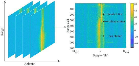
Figure 1.
Example of an RD map.
Sea clutter is generated by the interaction between radar signals and ocean waves. The first-order Bragg peak observed in sea clutter arises from the interaction between the high-frequency electromagnetic waves transmitted by OTHR and the Bragg resonance scattering caused by ocean waves [17]. Generally, sea clutter exhibits a symmetrical dual peak around the 0 Hz frequency in an RD map, as shown in Figure 2. Land clutter is generated by the interaction between radar signals and the ground. The relative change in speed of ground targets is relatively small, often manifesting as low-speed signals, so the spectrum of land clutter is usually more stable [17]. Ideally, land clutter exhibits a single peak around the 0 Hz frequency in an RD map, as shown in Figure 2. Generally, mixed clutter occurs near the coastline, where the radar signals interact with both ocean waves and the ground [17]. Therefore, mixed clutter has the characteristics of both sea clutter and land clutter, as shown in Figure 2. When the ionosphere is stable, the amplitude of land clutter exceeds that of sea clutter due to the higher scattering coefficient of terrestrial surfaces compared to that of maritime surfaces, as shown in Figure 2. Human experts leverage these characteristics when classifying sea–land clutter data. Consequently, the features of sea–land clutter around the 0 Hz frequency play a crucial role in SLCC.
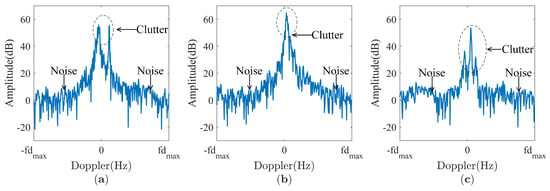
Figure 2.
Examples of clutter in an RD map. (a) Sea clutter. (b) Land clutter. (c) Mixed clutter.
2.2. Coordinate Registration
The CR parameters are crucial for target positioning with OTHR, which can improve the positioning accuracy. An SLCC-based CR method is the process of matching the SLCC results with an electronic map. Generally, the process of CR is divided into two steps: (1) converting the SLCC results from the radar coordinate system into the geographic coordinate system and (2) mapping the SLCC results onto the electronic map and finding the best-matching results.
OTHR transmitters and receivers are set up separately, and the distance between them is negligible [22]. Assume that the longitude and latitude of the radar receiver are . In the radar coordinate system, the azimuth and range of the target are and r, respectively. Then, the longitude and latitude of the target can be defined as follows:
where is defined as follows:
where R is the radius of the Earth. In fact, the Earth is not a ideal sphere but an ellipsoid. When considering the flatness and eccentricity of the Earth, a more accurate formula is needed [22]. And then C is defined as follows:
Each azimuth–range cell in the SLCC results contains the azimuth and range in the radar coordinate system. The longitude and latitude of each azimuth–range cell can be calculated using Equations (1)–(3). By mapping the longitude and latitude of all of the cells onto the electronic map, the CR parameters can be calculated, as shown in Figure 3. On the left-hand side of Figure 3, the azimuth–range cells labeled in blue, red, and green represent sea clutter, land clutter, and mixed clutter, respectively.
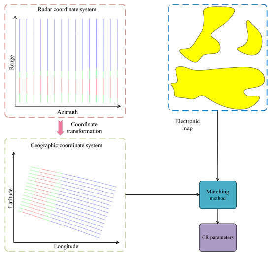
Figure 3.
Diagram of coordinate registration.
It is difficult to obtain accurate matching results due to the mixed clutter. Mixed clutter causes the coastline or island outlines in the SLCC results to differ from those in the electronic map. Further subdivision of the mixed clutter is necessary, which will be described in Section 3.2. It should be noted that in practical engineering applications, clutter class misjudgment is also an important factor affecting the accuracy of the CR parameters [13], which will be studied further in future work.
2.3. Graph Similarity Computation
In this section, we introduce the background related to the graph similarity computations. Let represent an undirected connected graph, where V is the set of all nodes and E is the set of all edges without a self-loop. The number of nodes in is . is a symmetric adjacency matrix which describes the relationships between nodes, and can be defined as follows:
where indicates the existence of an edge between nodes and , and .
Let denote the neighborhood set of node , i.e., . is the feature matrix, whose i-th row is a feature vector of node , and d is the dimension of the node feature. Let represent the label encoding matrix, whose i-th row is the one-hot encoding of the label of node , and is the number of classes.
Given and , the graph similarity computation aims to calculate the similarity score between and . In the graph similarity computation, the graph edit distance (GED) is a classic and important index used to assess the difference between two graphs [23]. Specifically, the GED calculates the minimum cost required to transform one graph into another through a series of graph editing operations, including insertion, deletion, and the replacement of nodes and edges, which can be formally summarized as follows:
where represents a set of graph editing operations which contains all of the graph editing operations required to transform into . represents the cost of operating u, depending on the type of graph editing operation. Obviously, if two graphs are identical (i.e., isomorphic), their GED is zero.
Figure 4 illustrates an example of calculating the GED between two graphs, where the value of the GED is 3. Transforming the graph from the left to the right requires three graph editing operations: (1) removing the edge between node 1 and node 4; (2) inserting an edge between node 1 and node 2; and (3) replacing the label for node 1.

Figure 4.
An example of the GED between a pair of graphs. The GED from the left to the right is 3 because the conversion requires 3 editing operations: (1) deleting an edge, (2) inserting an edge, and (3) relabeling a node.
Calculating the GED between two graphs is known to be NP-complete, and even state-of-the-art methods cannot reliably compute the exact GED between graphs with more than 16 nodes within a reasonable time frame [24]. Once the distance between two graphs has been calculated, we transform it into a similarity score ranging between 0 and 1. More details about the transformation function will be described in Section 4.2.
3. The Method
This section first introduces the details of converting the SLCC results into graph data, then presents a mixed clutter clustering method for subdividing mixed clutter, and finally describes the proposed SC-GNN and the implementation of CR.
3.1. Constructing the Graph
Any data in the normed space can be represented by graph data, i.e., non-Euclidean data [25]. Graphs are powerful data structures capable of capturing the relationships between objects [26]. To convert the SLCC results from Euclidean space into non-Euclidean space, it is necessary to analyze the correlation of the sea–land clutter between adjacent azimuth–range cells in the sea–land clutter data. Statistically, the absolute distance (AD), the cosine similarity (CS), and Pearson’s correlation coefficient (PCC) are employed to measure the correlation between adjacent azimuth–range cells [27]. This correlation is evaluated from three aspects: the difference in the signal energy, the difference in the signal direction, and the signal correlation. The experimental results demonstrate a relatively strong correlation between adjacent azimuth–range cells in the sea–land clutter data, as presented in Section 4.4.
The process of constructing the graph involves establishing the correspondence between the SLCC results and the nodes and defining the edges. After converting the SLCC results into a geographic coordinate system, each azimuth–range cell contains information on longitude and latitude. Therefore, each azimuth–range cell can be represented as a node in the graph, and the longitude and latitude can be used to represent the node features . An effective and efficient method is used to build the edges between nodes [27], as shown in Figure 5. In the radar coordinate system, assuming that is the central node, the first-order neighbors are found along the axis of the azimuth and the range, respectively, and undirected edges are built.
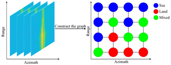
Figure 5.
Constructing the graph.
Furthermore, the process of converting the electronic map into graph data is as follows: (1) Let represent the SLCC results and represent the graph from the electronic map. Given the node , we search for the point closest to in the electronic map and define it as , establishing a one-to-one correspondence between the nodes in the two graphs. (2) We can assume a label for each node in based on the information in the electronic map. Obviously, and have the same number of nodes and edges. In the process of searching for the best match in the electronic map using the SLCC results, the longitude and latitude for each node in will change. We randomly select a detection area with and as an example; after converting the SLCC results from Euclidean space into the graph data, the number of nodes in the graph is 12,000, and the number of edges in the graph is 23,185.
3.2. Mixed Clutter Clustering
It is an important step to further divide the mixed clutter into sea clutter or land clutter to calculate the CR parameters. Mixed clutter may result in large differences between the coastlines or islands in the SLCC results and the electronic map. According to radar principles, the ocean and the ground are continuous in the OTHR detection area. Specifically, sea clutter is more likely to occur near sea clutter, and conversely, land clutter is more likely to occur near land clutter. This is also consistent with the homophily assumption in the graph data: nodes connected to each other tend to share similar properties, which is additional information in addition to the features of the nodes [28]. Therefore, the K-nearest neighbors-based mixed clutter clustering (KNN-MCC) method is proposed for dividing the mixed clutter further. The core idea of KNN-MCC is as follows: to classify the data, the distances between them and samples of known classes are calculated, and the nearest K samples are selected. According to the classes of the K samples, voting is conducted to decide the class of data for classification [29].
Let represent the SLCC results, and divide into a training set and a test set by classes. All of the nodes in the training set are represented as , which contains labeled sea clutter and land clutter. For each , the longitude is , and the latitude is . Similarly, all of the nodes in the test set are represented as , which contains labeled mixed clutter. For each , the longitude is and the latitude is . The KNN-MCC method consists of two steps: (1) we find the K nodes from the training set O which are closest to node , and (2) we vote on the classes of the K samples to subdivide the mixed clutter further into sea clutter or land clutter, as shown in Figure 6. Given the longitude and latitude of two nodes, the Haversine formula is used to calculate the distance between these two nodes [30], which is defined as follows:
where is the radian distance between the two nodes, is the longitude and latitude of , is the longitude and latitude of , and is the distance between the two nodes. Because sea clutter and land clutter originate from the ocean and the ground, respectively, altitude is ignored [22].
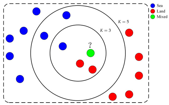
Figure 6.
A diagram of KNN-MCC. Blue dots represent the sea clutter, red dots represent the land clutter and green dots represent the mixed clutter.
After the SLCC results are processed using KNN-MCC, the mixed clutter is further subdivided into sea clutter or land clutter. The SLCC results can be binarized, which is convenient for registration with the electronic map. The details of KNN-MCC are shown in Algorithm 1. In the process of KNN-MCC, the radar parameters associated with the detection area are known, and the distance between nodes can be calculated in advance. In addition, the graph can be divided into a number of subgraphs to accelerate the computation. This allows the K-nearest neighbor search of to be carried out in each subgraph rather than in [29].
| Algorithm 1 The KNN-MCC implementation process. |
| Input: The SLCC results . Output: The SLCC results after clustering. 1: Initialize: The training set ; 2: The test set . 3: for do 4: for do 5: Calculate between and . 6: end for 7: Sort: Arrange all of the training samples in ascending order of . 8: Select neighbors: Select the first K neighbors with the smallest distance. 9: Vote: Vote to determine the label for based on the first K neighbors. 10: end for 11: return . |
3.3. Similarity Computation via a Graph Neural Network
In this article, we complete the CR task by calculating the similarity scores between graphs. Given a pair of undirected and unweighted graphs and , we aim to train a neural network whose input is two graphs and whose output is their similarity score. The similarity score can be mapped one to one back to the GED. SC-GNN consists of four parts—(1) graph segmentation, (2) subgraph-level embedding, (3) node-level comparison, and (4) calculating the similarity score—as shown in Figure 7.

Figure 7.
An overview illustration of SC-GNN.
3.3.1. Graph Segmentation
Most GNN-based graph similarity models employ mechanisms for generating both graph-level and node-level embeddings and compute the similarity scores between different graphs by combining the coarse-grained graph-level interactions with fine-grained node-level comparisons [23]. However, the above methods may have the following limitations in achieving CR tasks.
(1) There can be a lot of land and many islands in the OTHR detection area, and the terrain can be complex. Graph-level embeddings may have a limited capacity to represent the entire graph. In some cases, it is crucial to consider the local structural features.
(2) The OTHR detection area is wide. The large number of nodes results in high computational costs for node-level comparisons, and excessive matching of distant nodes may introduce noise.
Therefore, to represent the local structural features of the SLCC results better and reduce the computation, we divide the graph into q subgraphs of an equal size based on the region. And then , and . satisfies , where . In a CR task, human experts can set different q values for various detection areas due to the varying amounts of land and numbers of islands in each area.
3.3.2. Subgraph-Level Embedding
Both the subgraph-level embeddings and node-level comparisons necessitate computation of the node embeddings. Among the existing GNN methods, we chose a graph isomorphism network (GIN) because of its powerful capabilities in node aggregation and capturing graph structures [31]. Given , the process of node aggregation and updates in the GIN is defined as follows:
where is the node embedding for at layer , is the dimension of the node embedding at layer , MLP represents a multi-layer perceptron (MLP), is a learnable parameter, and is the neighbor nodes of . By stacking the GIN layers, the information from higher-order neighbors can be captured. Subsequently, the node-level embedding information is fed into the attention module.
To generate subgraph-level embeddings, the weighted average or weighted sum of the node embeddings can be computed. However, more important nodes should be assigned higher weights within the subgraph. Therefore, an attention mechanism is employed to learn the importance of the nodes in the subgraph. For ease of description, let denote the node embeddings of the GIN output. Firstly, a global graph context is computed as the average of the node embeddings, followed by a nonlinear transformation, , where is the learnable weight matrix. contains the global information on the subgraph and the feature information for calculating the similarity. For each , the attention weight can be calculated according to the inner product of and , followed by the Sigmoid function . can limit the attention weight to . Finally, the subgraph-level embedding is the weighted sum of the node embeddings, which can be defined as follows:
Through node embedding and the attention mechanism, we complete the subgraph-level embedding. Given the subgraph-level embeddings and , the CS can be used to measure the similarity between them, which can be defined as follows:
where ⊙ represents the dot product between vectors, and is the 2-norm of .
After dividing a pair of graphs into q subgraphs, the similarity between the subgraphs can be calculated using Equation (9). And then, the MLP is used to map the similarity scores between subgraphs to the coarse-grained similarity score, which is defined as follows:
where ⊕ represents the concatenation operation, and is the coarse-grained similarity score between and .
3.3.3. Node-Level Comparison
Subgraph-level embedding may lose fine-grained information. Computing all pairs of subgraphs requires a lot of computation. Therefore, the y pairs of subgraphs with the highest scores are chosen for computing node-level comparisons. Take a pair of subgraphs and , where and . The nodes within each subgraph and the nodes between subgraphs are compared separately. Within each subgraph, the node embedding is updated for t rounds, and the influence of on is defined as follows:
where or .
For node interactions between subgraphs, the attention mechanism is used to calculate the importance of to , which is defined as follows:
where or . The attention mechanism can capture more similar nodes in a pair of subgraphs. The influence of on is defined as follows:
3.3.4. Similarity Score Calculation
In the process of graph segmentation, each graph is divided into q subgraphs, and pairs of subgraphs are generated. The subgraph-level similarity scores are sorted, and the y pairs of subgraphs with the highest scores are obtained for node-level comparisons. We use coarse-grained scores and y fine-grained scores to obtain the final similarity score between graphs, which is defined as follows:
After the predicted value is obtained, the mean squared error loss function is used to compare it with the ground truth similarity score, which is defined as follows:
where is the set of training graph pairs, is the number of training graph pairs, and is the ground truth similarity between and .
3.4. The Coordinate Registration Process Based on Similarity Computations
The calculation method for the CR parameters based on SC-GNN mainly includes the following steps: (1) The sea–land clutter data are fed into the trained high-performance classifier, and the SLCC results are produced as output. (2) The SLCC results are converted into the geographic coordinate system and prior information from human experts used to narrow the search area of the SLCC results in the electronic map. (3) The SLCC results and the electronic map are converted into graph data, and then the mixed clutter is subdivided into sea clutter or land clutter using KNN-MCC. (4) SC-GNN is used to search for the best-matching region of SLCC results, and the CR parameters are calculated. This process is shown in Figure 8. Assuming that has been matched with in the geographic coordinate system, and are the corresponding nodes, and the CR parameters are defined as follows:
where is the longitude and latitude of , and is the longitude and latitude of .
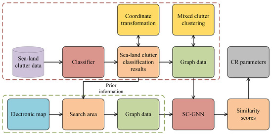
Figure 8.
Flowchart of CR parameter calculation via SC-GNN.
4. Results and Discussion
In this section, we first introduce the experimental datasets, the experimental environment, the experimental parameter settings, and the evaluation indexes. Secondly, the comparison methods are described in detail. Finally, the effectiveness of KNN-MCC and SC-GNN are verified on the given datasets.
4.1. Datasets
To verify the feasibility of converting sea–land clutter data from Euclidean space into graph data in non-Euclidean space, we build the original sea–land clutter dataset. Six detection areas are randomly selected for building the original sea–land clutter dataset: (1) Area-1, (2) Area-2, (3) Area-3, (4) Area-4, (5) Area-5, and (6) Area-6. To ensure the diversity of the samples and the stability of the results, for each detection area, 10 groups of sea–land clutter samples from different ionospheric conditions, different seasons, and different times are randomly selected. Due to the high non-stationarity of sea–land clutter, the original sea–land clutter dataset includes sea–land clutter samples from various typical scenes so as to ensure the complex OTHR environment is completely characterized as much as possible. In addition to the examples of sea–land clutter in Figure 2, the original sea–land clutter dataset also contains samples from relatively complex environments, such as sea–land clutter samples with Doppler frequency shifts, amplitude fluctuations, and narrowband radio frequency interference (NRFI), as shown in Figure 9. To perform different types of tasks, OTHR dynamically adjusts the detection area and the working parameters, and the quantity and relative position of the land clutter, sea clutter, and mixed clutter in the RD map also change. The original sea–land clutter dataset contains a total of 60 groups of samples. The number of instances of sea–land clutter in each group is , and the dimension of sea–land clutter is 512.
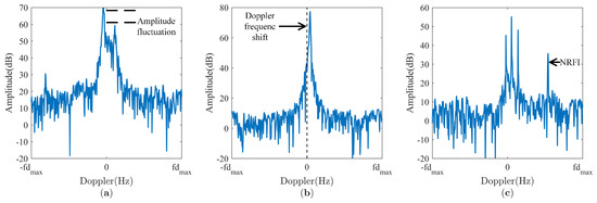
Figure 9.
Examples of clutter in an RD map. (a) Sea clutter with amplitude fluctuations. (b) Land clutter with Doppler frequency shifts. (c) Mixed clutter with NRFI.
To verify the effectiveness of KNN-MCC, we build a sea–land clutter cluster dataset, whose detection areas are the same as those of the original sea–land clutter dataset. Building the sea–land clutter cluster dataset involves three steps: (1) According to the radar parameters (azimuth, range, azimuth resolution, range resolution), the detection area is converted from the radar coordinate system into a geographic coordinate system and then mapped onto the electronic map. (2) For each azimuth–range cell, the nearest location of the ocean or the ground is searched for in the electronic map, and label information is obtained (the sea is labeled as 0, and the land is labeled as 1). (3) At junctions between the ocean and the ground, labels for mixed clutter are generated with a certain probability, which are labeled as 2. For each azimuth–range cell, the closer the distance is to the boundary, the greater the probability of distinguishing it as mixed clutter. To ensure the diversity of the samples and the reliability of the experimental results, 200 groups of SLCC results are randomly generated for each detection area. Therefore, the sea–land clutter cluster dataset contains 1200 groups of SLCC results and their corresponding ground truths. In the sea–land clutter cluster dataset, cells labeled as sea and land clutter are used as the training set, and cells labeled as mixed clutter are used as the test set. The proportion of sea and land in the above six detection areas in the electronic map is shown in Figure 10. Through the generation of appropriate samples and the use of diverse regional settings, the sea–land clutter cluster dataset provides a robust foundation for evaluating the performance of KNN-MCC in complex environments.
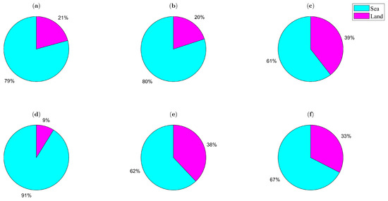
Figure 10.
The proportion of sea and land in the electronic map. (a–f) represent the proportion of sea and land for Area-1 to Area-6, respectively.
Moreover, to verify the effectiveness of SC-GNN, we build a sea–land clutter registration dataset based on the sea–land clutter cluster dataset. Specifically, building the sea–land clutter registration dataset involves four steps: (1) Using the sea–land clutter cluster dataset as the input, the mixed clutter in the SLCC results is effectively classified into sea clutter and land clutter using KNN-MCC. After clustering, the SLCC results contain only sea and land clutter, facilitating binarization. (2) The longitude and latitude offsets, i.e., the CR parameters, are added to each group of samples based on the prior information. (3) For each group of SLCC results in the sea–land clutter registration dataset, the search range is determined based on prior knowledge provided by human experts. Next, the GEDs between the SLCC results and the subareas of the electronic map are computed individually and converted into similarity scores, which are treated as the truth values. (4) Each detection region in the sea–land clutter registration dataset contains 200 groups of SLCC results; 60% of the samples are randomly allocated into the training set, 20% into the validation set, and the remaining 20% into the test set, as shown in Table 1. Therefore, the sea–land clutter registration dataset contains six detection areas, with each area containing 200 groups of SLCC results and the corresponding search area in the electronic map. Each group of samples is converted into graph data according to the method proposed in Section 3.1. The number of nodes and the number of edges in the graph are and , respectively. Typically, graph data are stored in binary file format.

Table 1.
The settings of the sea–land clutter registration dataset.
4.2. The Parameter Settings and Evaluation Indexes
The experimental environment for KNN-MCC and SC-GNN is shown in Table 2. For the proposed architecture of SC-GNN, each graph is divided into q (here ) subgraphs. Among all 16 subgraph pairs, 0, 8, and 16 subgraph pairs with the highest similarity scores are selected for node-level comparisons. These models are called SC-GNN-sl (the similarity scores are calculated using only the subgraph-level embeddings), SC-GNN-y (the top y or eight subgraph pairs with the highest scores are selected for the node-level comparisons), and SC-GNN (we select all subgraph pairs for the node-level comparisons), respectively. Compared with SC-GNN-sl, SC-GNN and SC-GNN-y use all subgraph pairs and some of the subgraph pairs, respectively, for the node-level comparisons. This comparison can be regarded as an ablation experiment.

Table 2.
The experimental environment.
The number of GIN layers is set to 3, and a parametric rectified linear unit (PReLU) is used as the activation function. If the number of layers is too high, oversmoothing may occur, leading to a reduced ability to distinguish between different nodes. The dimensions of the node embedding at layers 1, 2, and 3 are 64, 32, and 16, respectively. The dimension of the similarity vector obtained in the subgraph-level embedding stage is reduced from 16 to 8 by using the fully connected layer, and the dimension of the similarity vector obtained in the node-level comparison stage is 8 in using the fully connected layer. Finally, the dimensions of the connection results of the subgraph-level embedding module and the node-level comparison module are reduced to 1 by using four fully connected layers.
In the training process, the batch size is set to 16, and the model carries out 2000 epochs of parameter update iterations on the training set. The model with the lowest loss is chosen as the best model. The Adam method is used to optimize the loss function, with Beta1 set to 0.5, Beta2 set to 0.999, and the learning rate set to 0.001. The input to the model is a pair of graphs, and the output is the similarity score for this pair of graphs. The experimental parameters of the comparison methods are consistent. To prevent overfitting of the model, the performance of the model is evaluated using cross-validation, and suitable hyperparameters are selected to ensure the generalization ability of the model.
Given a pair of graphs, and , converting the computed GED into a similarity score involves two steps. First, we normalize the GED by , where is the number of nodes in . And then, we use the exponential function to map the to [0, 1], representing the similarity of the pair of graphs. It can be observed that as decreases, the similarity between the pair of graphs increases, approaching 1.
The mean absolute error (MAE) and the mean squared error (MSE) are used to evaluate the similarity calculation results of SC-GNN. The MAE is the average of the absolute difference between the calculated similarities and the ground truth similarities, which is used to measure the average error of the model. The MSE is the average of the square of the difference between the calculated similarities and the ground truth similarities, which is more sensitive to large errors and can highlight significant deviations. Moreover, for the ranking results, Spearman’s rank correlation coefficient [32] () and Kendall’s rank correlation coefficient [33] () are used to evaluate the matching performance of the predicted ranking results with the true ranking results. Spearman’s rank correlation coefficient measures the correlation by measuring the monotonic relationship between the predicted ranking results and the actual ranking results. Kendall’s rank correlation coefficient measures relevance by measuring the sequential consistency of the predicted ranking results with the real ranking results. The precision at k (p@k) is calculated by taking the intersection of the predicted top k results and the ground truth top k results divided by k. Compared with p@k, and pay more attention to the global ranking results than to the top k results.
In addition, accuracy (AC), precision (PE), recall (RE), and F1 values are used to evaluate the classification performance of KNN-MCC on the sea–land clutter cluster dataset. To ensure the reliability of the experimental results, the experiment is conducted on 10 groups of samples from each detection area, and the average performance is recorded. In calculating the above indexes, the land clutter is treated as a positive sample.
4.3. Comparison Methods
Our baseline includes two categories of methods, graph-embedding-based methods and graph-matching-network-based methods.
- The first category includes two graph embedding models based on graph convolutional networks (GCNs) [34], GCN-Mean and GCN-Max [35]. The above methods embed graphs into vectors using a GCN and subsequently use the similarities computed from these vectors as the similarity scores for the graph pairs.
- The second category includes two graph matching networks, similarity computation via a graph neural network (Sim-GNN) [24] and graph matching networks (GMNs) [36]. Sim-GNN integrates the embedding of the entire graph with the node-level comparisons. GMNs leverage the information from the comparison nodes both within individual graphs and across different graphs to compute the similarity.
4.4. The Correlation Analysis on the Original Sea–Land Clutter Dataset
The AD, CS, and PCC are used to evaluate the correlation between adjacent azimuth–range cells in the original sea–land clutter dataset. The value for the AD is positive, indicating the difference in the signal energy between adjacent azimuth–range cells. The closer the AD is to 0, the stronger the correlation between adjacent azimuth–range cells is. Before calculating the AD between adjacent azimuth–range cells, the signal amplitudes of all of the cells need to be normalized. The value of the CS ranges from −1 to 1. As the CS approaches 1, the difference in the direction between adjacent azimuth–range cells decreases, and the correlation strengthens. Generally, when the value of the CS is at least 0.6, two signals are strongly correlated [37]. The value of PCC ranges from −1 to 1. The closer the PCC is to 1, the stronger the signal correlation of the adjacent azimuth–range cells is. Generally, when the value of PCC is no less than 0.6, two signals are strongly correlated [37]. Then, the above indexes between adjacent azimuth–range cells in the original sea–land clutter dataset are calculated along the azimuth axis and the range axis, respectively, and the average values are calculated for each detection area, as shown in Table 3. A group of sea–land clutter samples is randomly selected from the original sea–land clutter dataset and displayed visually, as shown in Figure 11.

Table 3.
Correlation analysis on the original sea–land clutter dataset.
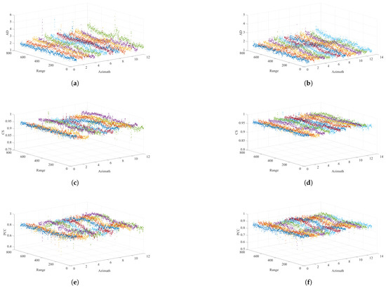
Figure 11.
Correlation of adjacent azimuth–range cells. (a) The absolute distance on the azimuth axis. (b) The absolute distance on the range axis. (c) The cosine similarity on the azimuth axis. (d) The cosine similarity on the range axis. (e) Pearson’s correlation coefficient on the azimuth axis. (f) Pearson’s correlation coefficient on the range axis.
The above results show that the samples in the original sea–land clutter dataset have a relatively strong correlation on the azimuth axis and the range axis. Therefore, adjacent azimuth–range cells can be connected by an edge, and the sea–land clutter data can be converted from Euclidean space into graph data in non-Euclidean space according to the method for constructing a graph proposed in Section 3.1.
4.5. The KNN-MCC Analysis on the Sea–Land Clutter Cluster Dataset
Table 4 summarizes the experimental results of KNN-MCC on the sea–land clutter cluster dataset with six detection areas. It can be seen that the proposed KNN-MCC performs well in all indexes on the sea–land clutter cluster dataset. In all detection areas, the AC is no less than 97.91%, the PE is no less than 97.52%, the RE is no less than 97.21%, and the F1 value is no less than 97.52%. This implies that KNN-MCC is powerful, showing the efficacy of the nearest neighbor mechanism, which can make full use of the label information from neighbor nodes. Generally, in the RD map, the mixed clutter that is closer to the sea clutter has a greater probability of being distinguished as sea clutter. Similarly, the mixed clutter that is closer to the land clutter has a higher probability of being identified as land clutter. The visualization results for KNN-MCC on the sea–land clutter cluster dataset are shown in Figure 12. It can be seen that after the mixed clutter is subdivided into sea clutter and land clutter, the terrain’s contours are clearer, and the shape features are more significant.

Table 4.
Classification indexes for KNN-MCC on the sea–land clutter cluster dataset.
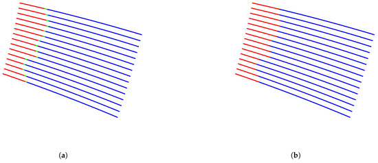
Figure 12.
Visualization of KNN-MCC on the sea–land clutter cluster dataset. Blue dots represent sea clutter, red dots represent land clutter, and green dots represent mixed clutter. (a) SLCC results before mixed clutter clustering. (b) SLCC results after mixed clutter clustering.
Moreover, to verify the rationality of KNN-MCC, its specific hyperparameters are discussed. Specifically, the value of K in KNN-MCC is quantitatively analyzed. Area-2 in the sea–land clutter cluster dataset is randomly selected for a comparative experiment. We gradually increase K from 3 to 11 to capture more information on the neighbor nodes from the SLCC results. As shown in Figure 13, when K changes, the classification accuracy of KNN-MCC on the sea–land clutter cluster dataset fluctuates within a stable interval. Therefore, the value of K is set to 5, which is common in practical applications.
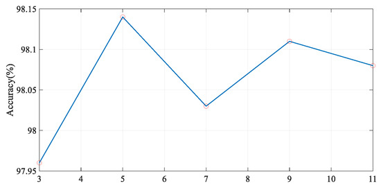
Figure 13.
Classification accuracy (%) of different K values on the sea–land clutter cluster dataset.
4.6. A SC-GNN Analysis on the Sea–Land Clutter Registration Dataset
Table 5, Table 6, Table 7, Table 8, Table 9 and Table 10 summarize the experimental results of SC-GNN on the sea–land clutter registration dataset. It can be seen that the proposed SC-GNN performs the best in all indexes on the sea–land clutter registration dataset with different areas. SC-GNN considers both subgraph-level interactions and node-level interactions, which not only can effectively capture the local structural features of the SLCC results and the electronic map but can also conduct fine node-level comparisons of the y pairs of subgraphs with the highest similarity scores. In all detection areas, is no less than 0.800, is no less than 0.639, p@10 is no less than 0.706, and p@20 is no less than 0.845. This means that in the electronic map, matching results that are more similar to the SLCC results are reliable. The above matching results can be used to calculate the CR parameters, which can help experienced human experts make decisions.

Table 5.
Experimental results for Area-1 in the sea–land clutter registration dataset.

Table 6.
Experimental results for Area-2 in the sea–land clutter registration dataset.

Table 7.
Experimental results for Area-3 in the sea–land clutter registration dataset.

Table 8.
Experimental results for Area-4 in the sea–land clutter registration dataset.

Table 9.
Experimental results for Area-5 in the sea–land clutter registration dataset.

Table 10.
Experimental results for Area-6 in the sea–land clutter registration dataset.
Compared with SC-GNN-sl and SC-GNN-y, SC-GNN considers all possible subgraph-level comparisons. Although the computational cost of the model is increased, it can be seen from the experimental results that the performance of the model has been improved to different degrees in the six detection areas of the sea–land clutter registration dataset. The relative positions and proportions of sea and land vary across the six selected detection areas, and the terrain structure is complex. The sea–land clutter cluster dataset includes SLCC results from diverse scenarios. Despite these variations, SC-GNN performs effectively, demonstrating that the proposed method exhibits robustness and a strong generalization ability. Compared to SC-GNN-sl, SC-GNN-y uses the top y pairs of subgraphs with the highest similarity scores for node-level comparisons. However, in the different detection areas of the sea–land clutter registration dataset, each evaluation index for SC-GNN-y shows a certain degree of improvement. The experimental results show that the network structure of the proposed SC-GNN is reasonable and the node-level comparison module is effective. By adjusting the value of y in SC-GNN, the number of subgraph pairs requiring node-level comparisons can be flexibly adjusted, and the model shows certain extensibility. In the application of OTHR, SC-GNN can dynamically adjust the number of subgraph pairs used in the node-level comparisons based on the task requirements. If a task demands a higher matching accuracy, additional subgraph pairs can be incorporated into the comparison, thereby improving the model’s performance through increased computational effort. Conversely, if speed needs to be prioritized in a task, the computational load can be reduced, and only the top y pairs of subgraphs will be used in the node-level comparison.
Although SC-GNN-sl underperforms relative to SC-GNN-y and SC-GNN across all of the detection areas from the sea–land clutter registration dataset, its performance is comparable to that of Sim-GNN and GMN and superior to that of GCN-Mean and GCN-Max. This is due to the inclusion of a graph segmentation module in SC-GNN-sl. The SLCC results are divided into multiple subgraphs, which more effectively captures the local structural features, such as the terrain contours or sea–land boundary lines, while mitigating the noise interference caused by the excessive matching of distant nodes. The experimental results further validate the effectiveness of using subgraphs to compute graph similarity.
As shown in Table 5, Table 6, Table 7, Table 8, Table 9 and Table 10, SC-GNN exhibits a more flexible network structure and a superior matching performance compared to those of Sim-GNN and GMN. As the number of subgraph pairs in the node-level comparison module increases, the model captures more fine-grained information through node-level interactions, thereby progressively improving the performance. This outcome aligns with our expectations and further demonstrates the rationality and effectiveness of the network structure. Additionally, across all of the detection areas, GCN-Mean and GCN-Max underperformed compared to the other models in most of the evaluation metrics. The wide detection area in OTHR, coupled with the complex terrain and the large number of nodes in the SLCC results, limits the effectiveness of using a single vector to represent the entire map, leading to a poor model matching performance.
In summary, SC-GNN effectively performs graph similarity calculations on the given sea–land clutter registration dataset, offering robust support for calculating the CR parameters in OTHR.
4.7. The Ablation Experiment
To verify the effect of KNN-MCC on SC-GNN, ablation experiments are performed on the sea–land clutter registration dataset. For clarity, when building the sea–land clutter registration dataset, if all of the mixed clutter is divided into sea clutter, it is denoted as M → S. If all of the mixed clutter is divided into land clutter, it is denoted as M → L.
Table 11 presents the experimental results for various mixed clutter clustering methods combined with SC-GNN. The experimental results show that when all of the mixed clutter is classified as either sea or land clutter, the performance of the model significantly declines. In scenarios where land or islands are present within the OTHR detection area, the sea–land clutter data contain hundreds or even thousands of instances of mixed clutter, resulting in nonlinear discrepancies between the SLCC results and prior geographic information, making it difficult to find the optimal matching area in the electronic map. The experimental results verify the effectiveness of KNN-MCC. Based on the idea of nearest neighbors, the mixed clutter in the sea–land data is more accurately classified into sea or land clutter, thereby minimizing the disparity between the SLCC results and the electronic map and enhancing the performance of SC-GNN. Consequently, preprocessing the SLCC results using KNN-MCC is essential.

Table 11.
Experimental results of different mixed clutter clustering methods on the sea–land clutter registration dataset.
4.8. A Time Complexity Analysis
The computational cost of SC-GNN is divided into three parts: (1) In the process of graph segmentation, we divide the graph into q subgraphs based on the region. This process needs to traverse all nodes, and its linear computation cost is . (2) In the process of subgraph-level embedding, the computational cost associated with the node-level embeddings and the subgraph-level embeddings is . Suppose the dimension of the subgraph-level embedding is d and each graph is divided into q subgraphs: the computational cost of the subgraph-level interactions is . It should be noted that in the process of the graph similarity search, the node embeddings and subgraph-level embeddings can be calculated in advance, which can significantly reduce the calculation cost. (3) In the process of node-level comparisons, based on the similarity scores obtained through the subgraph-level interactions, we select the top y subgraph pairs with the highest similarity scores for the node-level comparisons. The number of nodes in each subgraph is , and the computational cost of the node-level comparisons for a pair of subgraphs is . q can be treated as a hyperparameter to balance between time and accuracy. If , SC-GNN only calculates the coarse-grained subgraph-level similarity. Therefore, depending on the specific task requirements, a trade-off between time and accuracy can be made to select the optimal solution.
5. Conclusions
We have proposed a graph similarity calculation method based on graph segmentation under a GNN framework. The proposed SC-GNN was used to complete a graph similarity calculation task so as to obtain the CR parameters in OTHR. First, sea–land clutter data were converted into graph data and unified in a coordinate system. And then, to solve the problem of calculating the similarity of large graphs from the point of view of subgraphs, we took any two graphs as the input and output their similarity score. Compared with the existing graph matching methods, SC-GNN had the best performance in all indexes on the sea–land clutter registration dataset.
We have taken the first step towards the calculation of the CR parameters in OTHR using a GNN. SC-GNN was suitable for the graph similarity calculation task, including but not limited to calculating the CR parameters in OTHR. In some OTHR detection areas, only small islands are present, most of the sea–land clutter data are mixed clutter, and information on the geographic structure is limited. Future research may focus on these scenarios to provide deeper insights. In addition, human feedback needs to be incorporated into the training process to enhance the model’s understanding of human intentions. Combining SC-GNN with data enhancement methods is also expected to improve the model’s performance further.
Author Contributions
Conceptualization: C.L., Z.W., Q.P. and Z.S. Methodology: C.L., Z.W. and Q.P. Software: C.L., Z.W. and Z.S. Validation: C.L., Z.W. and Z.S. Formal analysis: C.L., Z.W. and Q.P. Investigation: C.L. and Z.W. Resources: C.L., Z.W., Q.P. and Z.S. Data curation: C.L. and Z.S. Writing—original draft preparation: C.L. Writing—review and editing: C.L., Z.W., Q.P. and Z.S. Visualization: C.L. and Z.W. Supervision: C.L. and Z.W. Project administration: C.L. and Z.W. Funding acquisition: Z.W. and Q.P. All authors have read and agreed to the published version of the manuscript.
Funding
This research was supported by the National Natural Science Foundation of China under grants 62473317 and 62233014.
Data Availability Statement
The datasets presented in this article are not readily available because the data are part of an ongoing study. Requests to access these datasets should be directed to the corresponding author.
Conflicts of Interest
The authors declare no conflicts of interest.
Abbreviations
The following abbreviations are used in this manuscript:
| OTHR | Sky-Wave Over-the-Horizon Radar |
| SLCC | Sea–Land Clutter Classification |
| CR | Coordinate Registration |
| DCNN | Deep Convolutional Neural Network |
| RD | Range–Doppler |
| GNN | Graph Neural Network |
| SC-GNN | Similarity Calculation via a Graph Neural Network |
| GED | Graph Edit Distance |
| AD | Absolute Distance |
| CS | Cosine Similarity |
| PCC | Pearson’s Correlation Coefficient |
| KNN-MCC | K-Nearest Neighbors-Based Mixed Clutter Clustering |
| GIN | Graph Isomorphism Network |
| MLP | Multi-Layer Perceptron |
| NRFI | Narrowband Radio Frequency Interference |
| PReLU | Parametric Rectified Linear Unit |
| MAE | Mean Absolute Error |
| MSE | Mean Squared Error |
| AC | Accuracy |
| PE | Precision |
| RE | Recall |
| GCN | Graph Convolutional Network |
| Sim-GNN | Similarity Computation via a Graph Neural Network |
| GMN | Graph Matching Network |
References
- Ji, X.; Li, J.; Yang, Q. Annual characteristic analysis of ionosphere reflection from middle-latitude HF over-the-horizon radar in the northern hemisphere. IEEE Trans. Geosci. Remote Sens. 2023, 61, 5104117. [Google Scholar] [CrossRef]
- Thayaparan, T.; Villeneuve, H.; Themens, D.R.; Reid, B.; Warrington, M.; Cameron, T.; Fiori, R. Frequency management system (FMS) for over-the-horizon radar (OTHR) using a near-real-time ionospheric model. IEEE Trans. Geosci. Remote Sens. 2022, 60, 5116011. [Google Scholar] [CrossRef]
- Guo, Z.; Wang, Z.; Hao, Y.; Lan, H.; Pan, Q. An improved coordinate registration for over-the-horizon radar using reference sources. Electronics 2021, 10, 3086. [Google Scholar] [CrossRef]
- Han, Y.; Yang, Z.; Chu, X. Research on the correction of ionospheric distortion for ship detection in OTHR. Mod. Rad 2003, 25, 5–8. [Google Scholar]
- Wheadon, N.; Whitehouse, J.; Milsom, J.; Herring, R. Ionospheric modelling and target coordinate registration for HF sky-wave radars. In Proceedings of the 1994 Sixth International Conference on HF Radio Systems and Techniques, York, UK, 4–7 July 1994; IET: London, UK, 1994; pp. 258–266. [Google Scholar]
- Turley, M.; Gardiner-Garden, R.; Holdsworth, D. High-resolution wide area remote sensing for HF radar track registration. In Proceedings of the 2013 International Conference on Radar, Adelaide, Australia, 9–12 September 2013; pp. 128–133. [Google Scholar]
- Jin, Z.L.; Pan, Q.; Zhao, C.H.; Zhou, W.T. SVM based land/sea clutter classification algorithm. Appl. Mech. Mater. 2012, 236, 1156–1162. [Google Scholar]
- Li, C.; Wang, Z.; Zhang, Z.; Lan, H.; Lu, K. Sea/land clutter recognition for over-the-horizon radar via deep CNN. In Proceedings of the 2019 International Conference on Control, Automation and Information Sciences (ICCAIS), Chengdu, China, 23–26 October 2019; pp. 1–5. [Google Scholar]
- Wu, B.; Liu, C.; Chen, J. A Review of Spaceborne High-Resolution Spotlight/Sliding Spotlight Mode SAR Imaging. Remote Sens. 2024, 17, 38. [Google Scholar] [CrossRef]
- Luo, B.; Cao, H.; Cui, J.; Lv, X.; He, J.; Li, H.; Peng, C. SAR-PATT: A Physical Adversarial Attack for SAR Image Automatic Target Recognition. Remote Sens. 2024, 17, 21. [Google Scholar] [CrossRef]
- Weng, Y.; Zhang, Z.; Chen, G.; Zhang, Y.; Chen, J.; Song, H. Real-Time Interference Mitigation for Reliable Target Detection with FMCW Radar in Interference Environments. Remote Sens. 2024, 17, 26. [Google Scholar] [CrossRef]
- Li, C.; Zhang, Y.; Wang, Z.f.; Lu, K.; Pan, Q. Cross-scale land/sea clutter classification method for over-the-horizon radar based on algebraic multigrid. Acta Electron. Sin. 2022, 50, 3021. [Google Scholar]
- Li, C.; Zhang, X.; Zhang, Z.; Pan, Q.; Bai, X.; Yun, T. Multiscale Feature Deep Fusion Method for Sea–Land Clutter Classification. IEEE Sens. J. 2024. [Google Scholar] [CrossRef]
- Jiang, W.; Zhang, Z.; Li, C.; Wang, Z. Deep embedded convolution clustering-based classification of clutter for over-the-horizon radar. Fire Control Command Control 2022, 47, 122–127. [Google Scholar]
- Zhang, X.; Wang, Z.; Lu, K.; Pan, Q.; Li, Y. Data Augmentation and Classification of Sea-Land Clutter for Over-the-Horizon Radar Using AC-VAEGAN. IEEE Trans. Geosci. Remote Sens. 2023, 61, 5104416. [Google Scholar] [CrossRef]
- Zhang, X.; Li, Y.; Pan, Q.; Yu, C. Triple Loss Adversarial Domain Adaptation Network for Cross-Domain Sea–Land Clutter Classification. IEEE Trans. Geosci. Remote Sens. 2023, 61, 5110718. [Google Scholar] [CrossRef]
- Zhang, X.; Wang, Z.; Ji, M.; Li, Y.; Pan, Q.; Lu, K. A sea–land clutter classification framework for over-the-horizon radar based on weighted loss semi-supervised generative adversarial network. Eng. Appl. Artif. Intell. 2024, 133, 108526. [Google Scholar] [CrossRef]
- Xiao, S.; Wang, S.; Dai, Y.; Guo, W. Graph neural networks in node classification: Survey and evaluation. Mach. Vis. Appl. 2022, 33, 4. [Google Scholar] [CrossRef]
- Cai, L.; Li, J.; Wang, J.; Ji, S. Line graph neural networks for link prediction. IEEE Trans. Pattern Anal. Mach. Intell. 2021, 44, 5103–5113. [Google Scholar] [CrossRef] [PubMed]
- Xie, Y.; Liang, Y.; Gong, M.; Qin, A.K.; Ong, Y.S.; He, T. Semisupervised graph neural networks for graph classification. IEEE Trans. Cybern. 2022, 53, 6222–6235. [Google Scholar] [CrossRef]
- Liao, W.; Bak-Jensen, B.; Pillai, J.R.; Wang, Y.; Wang, Y. A review of graph neural networks and their applications in power systems. J. Mod. Power Syst. Clean Energy 2021, 10, 345–360. [Google Scholar] [CrossRef]
- Chen, Z.; Wand, Y. Improvement of OTHR data processing using external reference sources. Mod. Radar 2005, 27, 24–27. [Google Scholar]
- Ling, X.; Wu, L.; Wang, S.; Ma, T.; Xu, F.; Liu, A.X.; Wu, C.; Ji, S. Multilevel graph matching networks for deep graph similarity learning. IEEE Trans. Neural Netw. Learn. Syst. 2021, 34, 799–813. [Google Scholar] [CrossRef]
- Bai, Y.; Ding, H.; Bian, S.; Chen, T.; Sun, Y.; Wang, W. Simgnn: A neural network approach to fast graph similarity computation. In Proceedings of the Twelfth ACM International Conference on Web Search and Data Mining, Melbourne, VIC, Australia, 11–15 February 2019; pp. 384–392. [Google Scholar]
- Veličković, P. Everything is connected: Graph neural networks. Curr. Opin. Struct. Biol. 2023, 79, 102538. [Google Scholar] [CrossRef] [PubMed]
- Zhou, J.; Cui, G.; Hu, S.; Zhang, Z.; Yang, C.; Liu, Z.; Wang, L.; Li, C.; Sun, M. Graph neural networks: A review of methods and applications. AI Open 2020, 1, 57–81. [Google Scholar] [CrossRef]
- Li, C.; Wang, Z.; Zhang, X.; Pan, Q. Land-sea clutter classification method based on multi-channel graph convolutional networks. J. Radars 2024, 14, 322–337. [Google Scholar]
- McPherson, M.; Smith-Lovin, L.; Cook, J.M. Birds of a feather: Homophily in social networks. Annu. Rev. Sociol. 2001, 27, 415–444. [Google Scholar] [CrossRef]
- Halder, R.K.; Uddin, M.N.; Uddin, M.A.; Aryal, S.; Khraisat, A. Enhancing K-nearest neighbor algorithm: A comprehensive review and performance analysis of modifications. J. Big Data 2024, 11, 113. [Google Scholar] [CrossRef]
- Saputra, K.; Nazaruddin, N.; Yunardi, D.H.; Andriyani, R. Implementation of haversine formula on location based mobile application in syiah kuala university. In Proceedings of the 2019 IEEE International Conference on Cybernetics and Computational Intelligence (CyberneticsCom), Banda Aceh, Indonesia, 22–24 August 2019; pp. 40–45. [Google Scholar]
- Xu, K.; Hu, W.; Leskovec, J.; Jegelka, S. How powerful are graph neural networks? arXiv 2018, arXiv:1810.00826. [Google Scholar]
- Spearman, C. The proof and measurement of association between two things. In Studies in Individual Differences: The Search for Intelligence; Jenkins, J.J., Paterson, D.G., Eds.; Appleton-Century-Crofts: New York, NY, USA, 1961. [Google Scholar]
- Kendall, M.G. A new measure of rank correlation. Biometrika 1938, 30, 81–93. [Google Scholar] [CrossRef]
- Kipf, T.N.; Welling, M. Semi-supervised classification with graph convolutional networks. arXiv 2016, arXiv:1609.02907. [Google Scholar]
- Defferrard, M.; Bresson, X.; Vandergheynst, P. Convolutional neural networks on graphs with fast localized spectral filtering. NeurIPS 2016, 29, 3844–3852. [Google Scholar]
- Li, Y.; Gu, C.; Dullien, T.; Vinyals, O.; Kohli, P. Graph matching networks for learning the similarity of graph structured objects. In Proceedings of the International Conference on Machine Learning, Long Beach, CA, USA, 9–15 June 2019; pp. 3835–3845. [Google Scholar]
- Niven, E.B.; Deutsch, C.V. Calculating a robust correlation coefficient and quantifying its uncertainty. Comput. Geosci. 2012, 40, 1–9. [Google Scholar] [CrossRef]
Disclaimer/Publisher’s Note: The statements, opinions and data contained in all publications are solely those of the individual author(s) and contributor(s) and not of MDPI and/or the editor(s). MDPI and/or the editor(s) disclaim responsibility for any injury to people or property resulting from any ideas, methods, instructions or products referred to in the content. |
© 2025 by the authors. Licensee MDPI, Basel, Switzerland. This article is an open access article distributed under the terms and conditions of the Creative Commons Attribution (CC BY) license (https://creativecommons.org/licenses/by/4.0/).