Technical Note

MAL-Net: Model-Adaptive Learned Network for Slow-Time Ambiguity Function Shaping

by
Jun Wang
1,
Xiangqing Xiao
2,3,4,
Jinfeng Hu
2,3,4,*,
Ziwei Zhao
2,3,4,
Kai Zhong
2,3,4 and
Chaohai Li
4
1
School of Mechanical and Electrical Engineering, Zhongshan Institute, University of Electronic Science and Technology of China, Zhongshan 528400, China
2
Yangtze Delta Region Institute, University of Electronic Science and Technology of China, Quzhou 324000, China
3
School of Information and Communication Engineering, University of Electronic Science and Technology of China, Chengdu 611731, China
4
Intelligent Terminal Key Laboratory of Sichuan Province, Yibin Institute of UESTC, Yibin 644000, China
*
Author to whom correspondence should be addressed.
Remote Sens. 2025, 17(1), 173; https://doi.org/10.3390/rs17010173
Submission received: 2 December 2024 / Revised: 29 December 2024 / Accepted: 3 January 2025 / Published: 6 January 2025
(This article belongs to the Special Issue Advances in Remote Sensing, Radar Techniques, and Their Applications)

Abstract

:
Designing waveforms with a Constant Modulus Constraint (CMC) to achieve desirable Slow-Time Ambiguity Function (STAF) characteristics is significantly important in radar technology. The problem is NP-hard, due to its non-convex quartic objective function and CMC constraint. Existing methods typically involve model-based approaches with relaxation and data-driven Deep Neural Networks (DNNs) methods, which face the challenge of dataimitation. We observe that the Complex Circle Manifold (CCM) naturally satisfies the CMC. By projecting onto the CCM, the problem is transformed into an unconstrained minimization problem that can be tackled using the CCM gradient descent model. Furthermore, we observe that the gradient descent model over the CCM can be unfolded as a Deep Learning (DL) network. Therefore, byeveraging the powerfulearning ability of DL and the CCM gradient descent model, we propose a Model-Adaptive Learned Network (MAL-Net) method without relaxation. Initially, we reformulate the problem as an Unconstrained Quartic Problem (UQP) on the CCM. Then, the MAL-Net is developed toearn the step sizes of allayers adaptively. This is accomplished by unrolling the CCM gradient descent model as the networkayer. Our simulation results demonstrate that the proposed MAL-Net achieves superior STAF performance compared to existing methods.

1. Introduction

Designing a constant modulus waveform to shape a desirable Slow-Time Ambiguity Function (STAF) is a key technology in radar systems [1,2,3,4]. Waveforms with desirable STAF characteristics play a critical role in enhancing the performance of radar systems for high-speed moving target detection [5,6,7,8], high anti-interference [9,10,11], and navigation positioning [12]. In practical application, Constant Modulus Constraint (CMC) is imposed on waveforms to improve transmitter efficiency to its maximum potential [13,14,15,16]. Therefore, waveform design to shape the desired STAF with CMC has attracted wide attention.
The problem is formulated as minimizing the quartic objective function with waveform CMC. The existing methods to solve this problem generally include model-based methods with relaxation and data-driven Deep Neural Networks (DNNs) methods with dataimitation.
Model-based relaxation methods primarily relax the objective function. Typically, to relax the fourth-order objective function, a Maximum Block Improvement (MBI) approach has been proposed [17], which generates plenty of random samples to address the CMC. However, given the extensive sample generation, the computational complexity can become prohibitive. To mitigate this complexity, a Majorization–Minimization (MM) approach has been developed, replacing the original objective function with a relaxed surrogate function [18,19]. Nevertheless, constructing an appropriate surrogate function poses a challenge. To further diminish the relaxation error, the UniAFSIM method has been devised, by integrating the MM method and the Gradient Projection (GP) algorithm [20]. This method employs the MM method to construct a quadratic surrogate function and then applies the GP algorithm to solve it. However, the combined processes of MM and GP entail significant computational expense for convergence. In an effort to reduce computational expenses, the Quartic Gradient Descent (QGD) approach based on the Complex Circle Manifold (CCM) has been developed [21]. This method utilizes the CCM gradient descent algorithm after objective relaxation with the weighted signal power term. However, the performance remains insufficient, due to relaxation. To tackle thisimitation, a Manifold Optimization Embedding with Momentum (MOEM) approach has been proposed [22], to solve the problem without relaxing the objective function. By introducing a momentum term, convergence can be accelerated, and performance can be enhanced. Nonetheless, selecting appropriate momentum parameters poses a challenge.
Recently, Deep Neural Networks (DNNs) have offered significant performance improvements in several real-world issues in signal, naturalanguage, and image processing, byearning massive network parameters (potentially millions) with massive training data sets [23,24]. For instance, ower Integrated Sidelobe Levels (ISLs) have been demonstrated via ResNet in a veryong sequence design [25], andower classification errors than human-level performance have been reported on the ImageNet dataset [26]. Nevertheless, when there is aack of training data, these DNNs approaches cannot perform well enough [27]. Moreover, DNNs are usually referred to as black boxes, and it can be difficult to grasp how they make their predictions.
Solving this problem is challenging, due to the non-convexity of both the quartic objective function and the Constant Modulus Constraint (CMC). Existing methods typically rely on model-based relaxation techniques, which canead to performance degradation, due to the relaxation of the objective function. Recently, Deep Neural Networks (DNNs) have achieved significant performance improvements in signal processing byearning millions of parameters fromarge training datasets. However, DNNs tend to perform poorly in scenarios withimited training data.
Despite these challenges, we find that both the Deep Learning and model optimization methods offer distinct advantages. Specifically, the Complex Circle Manifold (CCM) can naturally satisfy the CMC, allowing the use of gradient-based methods to solve the problem without relaxing the objective function over the CCM. Additionally, Deep Learning can adaptively update the step sizes of gradient descent algorithms, effectively addressing the issue of step size selection. Inspired by these insights, we propose the Model-Adaptive Learned Network (MAL-Net) method, which efficiently solves the problem without relaxing the objective function. In this approach, the problem is first reformulated as an Unconstrained Quartic Problem (UQP) over the CCM. Then, the MAL-Net is developed by unrolling the CCM gradient descent model into networkayers, where the step sizes for eachayer are adaptively updated through Deep Learning.
Our contributions mainly include the following:
  • The proposed MAL-Net method solves the problem without objective function relaxation: The proposed MAL-Net is designed by unrolling the CCM gradient descent model into networkayers, enabling relaxation-free optimization of the objective function over the CCM space. This approach effectively addresses the performance degradation commonly caused by objective function relaxation in most existing model optimization methods.
  • The proposed MAL-Net method adaptively updates the step sizes of each networkayer: In a MAL-Net, the step sizes for eachayer are adaptively updated through Deep Learning, overcoming the challenge of step size selection in conventional gradient-based methods. Furthermore, a MAL-Net only requires training a single parameter in eachayer, significantly reducing computational cost compared to DNN methods, which requireearning aarge number of network parameters.
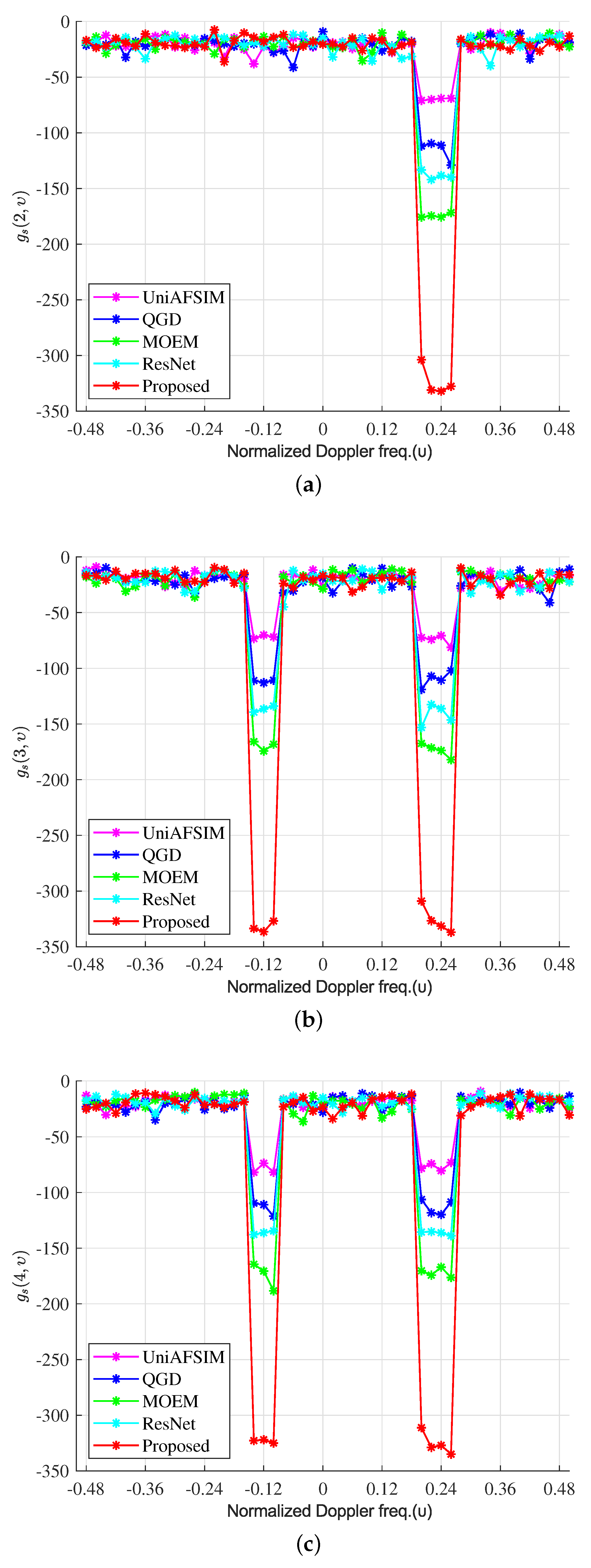
  • Compared with existing methods, the proposed MAL-Net method offers the following key improvements: (1) the nulls of the ambiguity function are decreased by 157 dB; (2) the Signal-to-Interference Ratio (SIR) gain is increased by 144 dB.
Notations: ( · ) H and ( · ) * represent Hermitian transpose and conjugate, respectively; E [ · ] denotes mathematical expectation; · represents taking an absolute value, and · represents the Euclidean norm; d i a g ( · ) means creating a diagonal matrix that uses vector elements as diagonal elements; ⊘ denotes element-wise deviation, and ⊙ denotes element-wise multiplication; · denotes taking an imaginary part of a vector, and · denotes taking a real part of a vector.

2. System Model

Consider a monostatic SISO radar system, which transmits a slow-time coded pulse; it is defined as
x = [ x ( 0 ) , x ( 1 ) , , x ( N 1 ) ] T C N ,
where N denotes the number of pulses.
Following down transformation to baseband and pulse matching filtering, the signal is sampled at the receiver. The receiver vector is expressed as
v = [ v ( 0 ) , v ( 1 ) , , v ( N 1 ) ] T C N ,
and
v = γ t x p ( v d t ) + d ( x ) + n ,
where γ t denotes the reflecting coefficient, v d t is the normalized Doppler frequency of target, and p ( v d t ) = [ 1 , e j 2 π v d t , , e j 2 π ( N 1 ) v d t ] T is the Doppler steering vector; n is the filtered noise vector with E [ n ] = 0 and E [ n n H ] = σ n 2 I . The vector of interfering echo samples, d ( x ) , is made up of the returns from N t distinct interfering scatterers that are spread across various range–azimuth bins. According to [20,21], d ( x ) is given by
d ( x ) = i = 1 N t β i J r i ( x p ( v d i ) ) = i = 1 N t β i J r i c v d i ,
where r i { 0 , 1 , , N 1 } is the range orientation, β i denotes the amplitude of the echo, and c v d i = x p ( v d i ) denotes the i-th scatterer’s signature, with v d i being the normalized Doppler frequency. The shift matrix J r i C N × N is given by
J r i ( a , b ) = 1 , a b = r i 0 , o t h e r w i s e ( a , b ) { 1 , , N } 2 .
where r i { N + 1 , , 0 , , N 1 } .
The target signature c v d t H v is obtained following the matched filter, which is defined as
c v d t H v = ( x p ( v d t ) ) H v = γ t x 2 2 + D ( r , x , v ) ,
where D ( r , x , v ) denotes the disruption at the output of the matched filter, which consists of noise and interference. It is given by
D ( r , x , v ) = c v d t H n + i = 1 N t β i c v d t J r i c v d i ,
Since d ( x ) is independent with n , the disruption energy is defined as
E D ( r , x , v ) 2 = E i = 1 N t β i c v d t J r i c v d i 2 + E c v d t H n 2 = r = 0 N 1 h = 0 N v 1 p ( r , h ) x 2 g x ( r , v h ) + σ n 2 x 2 ,
where p ( r , h ) denotes the interference map with respect to the range-Doppler bin, r { 0 , 1 , , N 1 } , h { 0 , 1 , , N v 1 } , and v h = 1 2 + h N v is the normalized frequency, while normalization means that the Doppler frequency interval is evenly divided into N v parts. And g x ( r , v h ) is the STAF, which is given by
g x ( r , v h ) = 1 x 2 x H J r c 2 .

3. Problem Formulation and Analysis

Our aim is to design a waveform that shapes the STAF to match the desired STAF. To reduce the hardware complexity and maximize the efficiency of the radar transmitter, the CMC is usually enforced on the waveform [28,29,30]. Given the CMC, x 2 in (9) is constant. Therefore, according to (9), the cost function can be given by
f ( x ) = r = 0 N 1 h = 0 N v 1 p ( r , h ) x 2 g x ( r , v h ) = r = 0 N 1 h = 0 N v 1 p ( r , h ) x H J r d i a g ( p ( v h ) ) x 2 = r = 0 N 1 h = 0 N v 1 x H p ( r , h ) J r d i a g ( p ( v h ) ) x 2 = i = 1 N × N v x H C i x 2 = i = 1 M x H C i x x H C i H x , ,
where C i = p ( r , h ) J r d i a g ( p ( v h ) ) , i = r N v + h , with i representing the range-Doppler bin ( r , h ) { 0 , , N 1 } × { 0 , , N v 1 } , and M = N × N v .
Combining (10) and the CMC, the problem can be formulated as [21]
min x f ( x ) = i = 1 M x H C i x x H C i H x s . t . x ( n ) = 1 , n = 1 , , N .
Note that (11) is challenging to solve, due to the non-convexity of both the quartic objective function and the CMC. In order to solve (11), the existing methods are generally model-based relaxation approaches, which may result in performance degradation due to the relaxation. Recently, DNNs have provided unprecedented performance gains in signal processing byearning massive network parameters (potentially millions) with massive training sets, while often performing poorly in situations withittle training data. Motivated by this, we propose a new method that combines the strengths of both the model-based and the DNNs-based methods. Concretely, a non-relaxation Model-Adaptive Learned Network (MAL-Net) method is derived byeveraging the powerfulearning ability of DL and the CCM gradient descent model.
The CCM is a geometric structure that inherently satisfies the Constant Modulus Constraint, allowing us to directly embed the constraint into the optimization process [31,32,33]. This eliminates the need for complicated constraint-handling techniques. Thus, we construct the manifold M to satisfy the CMC, which is given by [34,35,36,37,38]
M = x C N | x ( n ) = 1 , n = 1 , , N .
Hence, (11) can be reformulated as an Unconstrained Quartic Problem (UQP) over M , which is given by
min x M f ( x ) = i = 1 M x H C i x x H C i H x .

4. The MAL-Net Method

Note that (13) is an unconstrained minimization problem, which can be solved by the gradient descent model over the CCM. Furthermore, we note that the gradient descent model can be unfolded as a Deep Learning network, while the step sizes can be transformed intoearnable parameters. Hence, the Model-Adaptive Learned Network (MAL-Net) is proposed.

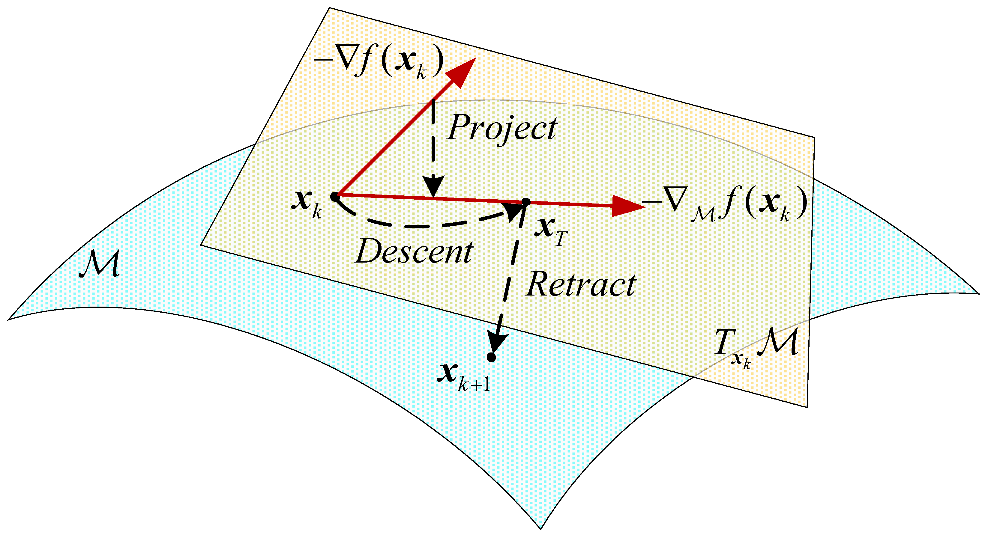
4.1. Gradient Descent Model over the CCM

Optimizing within the CCM ensures that the Constant Modulus Constraint is preserved throughout the iterative process. By using gradient-based methods, we can minimize the quartic function while staying within the manifold without relaxing the objective function, ensuring the validity of the optimization steps.
Figure 1 illustrates the gradient descent model over the CCM, which mainly includes three steps: (1) obtaining the Riemannian gradient by projection; (2) descent on the tangent space; (3) retraction to the CCM. Notably, in order to simplify the processing of Deep Learning, we transform complex variables into equivalent real-valued representations. The three steps are presented in detail as follows.

4.1.1. Obtaining the Riemannian Gradient by Projection

The Riemannian gradient at x k is defined as projecting the Euclidean gradient of x k onto the tangent space, which is given by
M f x k r = P T x k M f x k = f x k f x k x k * x k = f x k r ( Γ ) ( Γ )
where
  • T x k M , which is made up of all the tangent vectors at point x k , is a tangent space. It is defined as
    T x k M = z C L z x k * = 0 L .
  • P T x k M · denotes projection, from the Riemannian space to the tangent space at x k , which is defined as P T x k M a = a a x k * x k .
  • f x k r is the Euclidean gradient at the point x k . It is given by
    f ( x k ) = x k ( i = 1 M x k H C i x k x k H C i H x k ) = i = 1 M C i x k x k H C i H x k + ( x k H C i ) H ( x k H C i H x k ) H + x k H C i x k C i H x k + ( x k H C i x k x k H C i H ) H = 2 i = 1 M C i x k x k H C i H x k + C i H x k x k H C i x k = 2 i = 1 M ( c i ) ( x k ) ( c i ) ( x k ) i = 1 M ( c i ) ( x k ) + ( c i ) ( x k )
    where
    ( c i ) = Re _ a b + Re _ c d ( c i ) = Im _ a b + Im _ c d ,
    Re _ a b = Re _ a Re _ b Im _ a Im _ b Im _ a b = Re _ a Im _ b + Im _ a Re _ b Re _ c d = Re _ c Re _ d Im _ c Im _ d Im _ c d = Re _ c Im _ d + Im _ c Re _ d ,
    Re _ a = ( C i ) ( x k ) ( C i ) ( x k ) Im _ a = ( C i ) ( x k ) + ( C i ) ( x k ) Re _ b = ( C i ) ( x k ) ( C i ) ( x k ) T Im _ b = ( C i ) ( x k ) ( C i ) ( x k ) T ,
    Re _ c = ( C i ) T ( x k ) ( C i ) T ( x k ) Im _ c = ( C i ) T ( x k ) + ( C i ) T ( x k ) Re _ d = ( C i ) T ( x k ) ( C i ) T ( x k ) T Im _ d = ( C i ) T ( x k ) ( C i ) T ( x k ) T .
  • ( Γ ) and ( Γ ) are, respectively, defined as
    ( Γ ) = f x k ( x k ) ( x k ) + f x k ( x k ) ( x k )
    ( Γ ) = f x k ( x k ) ( x k ) + f x k ( x k ) ( x k ) .

4.1.2. Descent over Tangent Space

After performing the gradient descent, we obtain a tentative point on the tangent space, which is given by
x T r = ( x T ) ( x T ) = x k r α k M f x k r ,
where α k denotes the descent step size.

4.1.3. Retraction Back to the CCM

Retraction of x T back to the CCM generates the next feasible solution, which is
x k + 1 r = x T r x T x T ,
where x T is given by
x T = ( x T ) ( x T ) + ( x T ) ( x T ) .

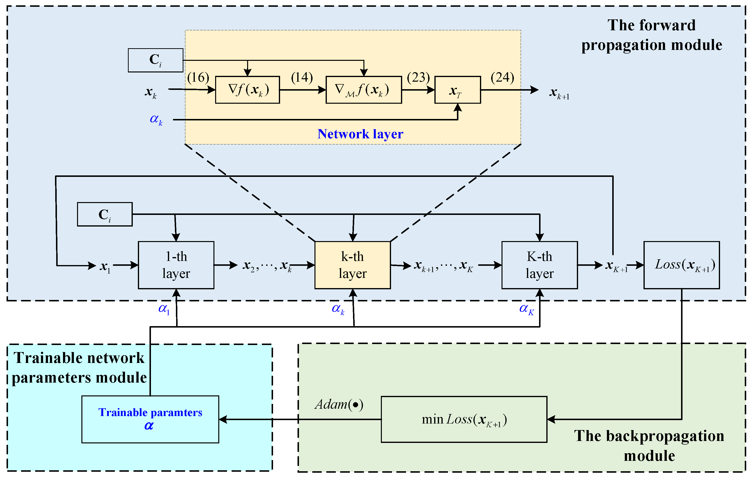
4.2. The Proposed MAL-Net

We note that the gradient descent model over the CCM for, specifically, (16), (14), (23), and (24) can be unfolded as the networkayer in Figure 2; then, a Deep Learning network is obtained. The core components of MAL-Net mainly include three aspects: the forward-propagation module, the backward-propagation module, and the parameters-training module. Assuming that all the network parameters are initialized, forward propagation can be employed for calculating theoss function. Then, backward propagation can be employed to minimize theoss function by the optimizer while training the network parameters.

4.2.1. Forward-Propagation Module

Each step of the gradient descent iteration can be considered as a forward pass in a neural network. This allows us toeverage the Deep Learning framework to optimize the problem, making use of automatic differentiation and parallel-computing techniques to improve efficiency. In addition, the step size can be adaptively updated by the Deep Learning framework, which is hard to determine in the conventional optimization method.
The forward-propagation module is made up of a gradient descent algorithm over the CCM; specifically, (16), (14), (23), and (24). Through K-layer network propagation, we obtain x k + 1 to compute theoss function, which is given by
L o s s = i = 1 M x H C i x x H C i H x = i = 1 M ( ψ i ) ( ψ i ) + ( ψ i ) ( ψ i ) ,
where
( ψ i ) = ( x ) T ( C i ) ( x ) + ( x ) T ( C i ) ( x ) + ( x ) T ( C i ) ( x ) ( x ) T ( C i ) ( x ) ,
( ψ i ) = ( x ) T ( C i ) ( x ) + ( x ) T ( C i ) ( x ) + ( x ) T ( C i ) ( x ) ( x ) T ( C i ) ( x ) .

4.2.2. Backward-Propagation Module

The network parameters are constantly optimized and adjusted by minimizing theoss function through back propagation, which facilitates the acceleration of convergence. It can be effectively realized by the Adam optimizer, which is widely used in Deep Learning for optimizing network parameters [39,40,41]. Using the trained parameters and the associated transforms, the final optimization variable values can be easily recovered when the training process is over.

4.2.3. Parameters-Training Module

Constant step size is usually chosen by the traditional gradient descent methods. Unlike these methods, the MAL-Net method sets the step sizes asayer-dependent trainable parameters, and it adaptively adjusts them through the powerfulearning ability of DL, which will accelerate the convergence, enhance the performance, and reduce the calculation cost. The trainable parameters in the network can be defined as α = [ α 1 , , α k , , α K ] T . Using the Adam optimizer to minimize theoss function, the descent step sizes can be adaptively adjusted to accelerate the convergence.
The MAL-Net method is summarized as Algorithm 1.
Algorithm 1 Model-Adaptive Learned Network (MAL-Net)
  • Input: C i , the networkayer K, the maximum number of iterations M a x i t e r , earning rate of Adam ϑ > 0 .
  • Output: x * = x n + 1 .
  • 1: Set the iteration index n = 0 and initialize α n , x n ;
  • 2: repeat
  • 3:  Set the networkayer k = 1 and x k = x n ;
  • 4:  repeat
  • 5:   Compute f ( x k ) by (16);
  • 6:   Compute M f ( x k ) by (14);
  • 7:   Compute x T by (23);
  • 8:   Update x k + 1 by (24);
  • 9:    k k + 1 ;
  • 10: until  k = K .
  • 11: return  x n = x K + 1 .
  • 12: Computeoss function by (26);
  • 13: Optimizeoss function with Adam optimizer;
  • 14: Update the step size α n + 1 ;
  • 15:  n n + 1 ;
  • 16: until  n > M a x i t e r .
  • 17: return  x n = x n + 1 .

4.3. Analysis of Complexity and Convergence

4.3.1. Analysis of Complexity

Calculating the Euclidean gradient f x k r of (16) and the L o s s of (26) forms the major computational complexity of a MAL-Net. Both the complexity of calculating f x k r and L o s s is O ( ξ N 2 ) , where ξ represents the total amount of interference. Therefore, in each iteration, the computational complexity is about O [ ( K + 1 ) ξ N 2 ] , where K represents the number of networkayers. We also provide theatest techniques for complexity comparison, such as the UniAFSIM method [20] with O ( N 3 + ξ N 2 ) , the QGD method [21] with O ( ξ N 2 ) , the MOEM method [22] with O ( ξ N 2 ) , and the ResNet method [25] with O ( ξ N 2 ) . As observed, the MAL-Net method exhibits comparable complexity to the QGD, MOEM, and ResNet methods, while demonstratingower complexity than the UniAFSIM method (per iteration).

4.3.2. Convergence Analysis

As Figure 2 shows, theoss function is calculated by forward propagation, and then the gradient of theoss function is obtained by backward propagation. Due to the complexity and nonlinearity of Deep Learning networks, there is no established theoretical proof for convergence.
In practice, the Adam optimizer is used to multiply the calculated gradient according to the presetearning rate, so as to update the trainable parameters α . Hence, the network parameters are constantly updated according to the gradient of theoss function along with the increasing number of iterations. The goal is to make theoss function continue to decline until it reaches convergence—that is, the change of theoss function value tends to remain steady, suggesting that theearning of the network model meets the preset convergence conditions. Thus, the proposed MAL-Net can achieve convergence practically.

5. Numerical Results

This section assesses the convergence, null STAF, Signal-to-Interference Ratio (SIR), and target detection performance. By way of comparison, methods including the UniAFSIM method [20], the QGD method [21], the MOEM method [22], and the ResNet method [25] are considered.
For convenience of comparison, we set the model configuration for simulation as [21]: we set v h = 1 2 + h N v , where h = 0 , , 49 and N v = 50 . Note that N v = 50 means normalizing the Doppler frequency interval to N v = 50 cells. We set the desired STAF as
p ( r , h ) = 1 , ( r , h ) { 2 , 3 , 4 } × { 35 , 36 , 37 , 38 } 1 , ( r , h ) { 3 , 4 } × { 18 , 19 , 20 } 0 , o t h e r w i s e .
The Signal-to-Interference Ratio (SIR) is a key performance metric that quantifies the ratio of the desired signal power to the interference power (the interference may include noise, jamming, or unwanted signals). A higher SIR indicates better signal quality, withess interference affecting transmission. In this section, we use the SIR to indicate the interference-suppression ability of the proposed MAL-Net method and other methods. The SIR can be given by [21]
SIR = N 2 r = 1 N h = 1 N v p ( r , h ) x 2 g x ( r , v h ) .

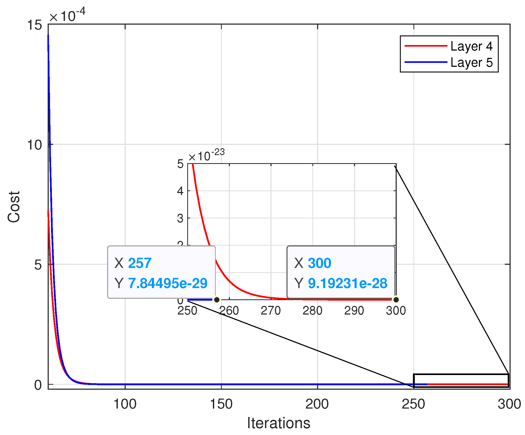
5.1. The Convergence Behavior

Figure 3 shows the convergence curves corresponding to differentayers of the network. As is evident, the proposed MAL-Net can converge to a fixed value, in terms of differentayers, andower cost is obtained as the number ofayers deepens. As shown in Figure 3, the cost values are 9.192 × 10 28 dB with fourayers and 7.845 × 10 29 with fiveayers, respectively.
In traditional gradient-based methods, ensuring convergence typically requires using very small step sizes, which ofteneads to more iterations with time-consuming computations. The small step size is necessary to guarantee stability and convergence, but it can significantly slow the optimization process. In contrast, the proposed method differs by adaptively updating the step size within the Deep Learning network. This adaptive adjustment allows the method to dynamically select an appropriate step size, which helps to accelerate convergence. As a result, the proposed approach typically converges to a good solution in a short time.

5.2. The Performance Comparison of Nulling STAF

Figure 4 exhibits a comparison of nulling the STAF for the UniAFSIM method [20], the QGD method [21], the MOEM method [22], the ResNet method [25], and the proposed method. It is obvious that the proposed MAL-Net method outperformed the current ones. The proposed MAL-Net method had theowest null asow as −326 dB. Specifically, the nulls reported in [20,21,22,25] were approximately 252 dB, 213 dB, 153 dB, and 188 dB higher than the proposed method, respectively.
Figure 5 shows the nulling STAF comparison with varying range cuts along r = 2 , 3 , 4 . As can be seen, the proposed MAL-Net achieved theowest nulls among all the methods. Specifically, at range cut r = 3, the nulls in [20,21,22,25] were approximately 255 dB, 218 dB, 157 dB and 189 dB higher than the proposed method, respectively.
These improvements demonstrate that the MAL-Net method exhibits a strong interference-suppression capability. Even in environments with strong interference, the MAL-Net maintains excellent target detection performance.

5.3. The Comparison of Time and SIR

Table 1 compares the computation time and Signal-to-Interference Ratio (SIR) for our proposed MAL-Net method and the methods of [20,21,22,25]. It is evident that the proposed MAL-Net method achieved the highest SIR. Specifically, the SIR of the MAL-Net was 301 dB, which showed improvements of 241 dB, 204 dB, 144 dB, and 177 dB over the methods in [20,21,22,25], respectively. The significant SIR improvements of the proposed MAL-Net compared to other methods demonstrate its superior ability to filter out unwanted signals, even in environments with strong interference. This enhanced interference suppression enables the MAL-Net to maintain excellent detection performance, ensuring more accurate and reliable target detection under challenging conditions.
In addition, the execution time of the MAL-Net is comparable to that reported in [21,25], and ateast two magnitudesower than that reported in [20]. In traditional gradient-based methods, convergence is typically ensured by using very small step sizes to maintain stability. However, this comes at the cost of slow convergence, as small step sizes significantly increase computation time. In contrast, the proposed MAL-Net method improves upon this by adaptively updating the step size within the Deep Learning framework. This dynamic adjustment allows the method to select an appropriate step size at each stage, accelerating the convergence process and reducing the time required to reach a good solution. One of the key advantages of the MAL-Net is its ability to optimize efficiently by only requiring the training of a single parameter perayer. This is a significant reduction in computational cost compared to traditional DNN methods, which typically requireearning aarge number of parameters. Overall, the combination of adaptive step size selection and reduced computational complexity makes the MAL-Net a more efficient approach for solving non-convex optimization problems, such as waveform design to match the required Slow-Time Ambiguity Function (STAF).

5.4. The Performance of Target Detection

We apply the optimized waveform to the target detection scenario, to show the superiority and practicability of the proposed method.
Consider a cognitive radar with transmit signal bandwidth B = 1 MHz, sample interval T s = 1 × 10 6 s, light speed c = 3 × 10 8 m/s, and working wavelength λ = 0.008 m. Assume that there are two high-speed targets in the target area, a strong target and a weak target, while the details are illustrated in Table 2:
The range–velocity plane for the Cross-Ambiguity Function (CAF) is given by
c ( r , f ) = h f H J r y 2 ,
where h f denotes the matched filter corresponding to f, which is expressed as
h f ( n ) = s * ( n ) e j 2 π f n ,
and y is the received echo, which is given by
y ( n ) = A s s ( n l s ) e j 2 π f s n +   A w s ( n l w ) e j 2 π f w n + v ( n ) ,
where v ( n ) is the Gaussian white noise variance with σ v 2 = 40 dB; A s denotes the amplitude of the strong target and A s 2 = 20 dB; A w represents the weak target and A w 2 = 60 dB.
Figure 6 shows the range–velocity planes of the CAF. As Figure 6a shows, the non-optimized waveform can detect strong targets, but not weak targets. Figure 6b shows that the optimized waveform, which is designed by the proposed MAL-Net, can detect both strong and weak targets.

6. Conclusions

This paper focuses on a waveform design for the STAF with the CMC. We propose a non-relaxation Model-Adaptive Learned Network (MAL-Net) method that combines the strengths of the gradient descent model over the CCM and the powerfulearning ability of DL. To be more specific, we first converted the problem into an Unconstrained Quartic Problem (UQP) over the CCM, which could be addressed via the gradient descent model. Then, the MAL-Net was designed to adaptivelyearn the step sizes by unfolding the manifold gradient descent model as the networkayer over the CCM. Our simulation results demonstrated that our proposed MAL-Net achieved superior STAF performance compared to the existing methods.

Author Contributions

Conceptualization, J.W. and J.H.; methodology, J.W., X.X. and Z.Z.; software, J.W. and K.Z.; validation, X.X., Z.Z. and K.Z.; formal analysis, J.W. and X.X.; investigation, X.X. and K.Z.; resources, J.H. and C.L.; data curation, C.L.; writing—original draft preparation, J.W.; writing—review and editing, J.W., Z.Z. and K.Z.; visualization, K.Z.; supervision, J.H.; project administration, J.W.; funding acquisition, J.H. All authors have read and agreed to the published version of the manuscript.

Funding

This work was supported by National Key R&D Program of China (NO. 2023YFF0717303), Key Areas Special Program for General Universities in Guangdong Province (New Generation Electronic Information) (NO. 2022ZDZX1047) and the Municipal Government of Quzhou (NO. 2023D040, 2023D009).

Data Availability Statement

Not applicable.

Acknowledgments

Thanks to the editor and all reviewers for their valuable comments.

Conflicts of Interest

The authors declare no conflicts of interest.

Abbreviations

The following abbreviations are used in this manuscript:
MIMOMultiple-Input Multiple-Output
STAFSlow-Time Ambiguity Function Shaping
CMCConstant Modulus Constraint
DNNsDeep Neural Networks
DLDeep Learning
UQPUnconstrained Quartic Problem
MBIMaximum Block Improvement
MMMajorization–Minimization
GPGradient Projection
QGDQuartic Gradient Descent
MOEMManifold Optimization Embedding with Momentum
ISLIntegrated Sidelobe Levels
MAL-NetModel-Adaptive Learned Network
SIRSignal-to-Interference Ratio

References

  1. Wang, X.; Li, B.; Chen, H.; Liu, W.; Zhu, Y.; Luo, J.; Ni, L. Interrupted-Sampling Repeater Jamming Countermeasure Based on Intrapulse Frequency–Coded Joint Frequency Modulation Slope Agile Waveform. Remote Sens. 2024, 16, 2810. [Google Scholar] [CrossRef]
  2. Song, Y.; Wang, Y.; Xie, J.; Yang, Y.; Tian, B.; Xu, S. Ultra-Low Sidelobe Waveforms Design for LPI Radar Based on Joint Complementary Phase-Coding and Optimized Discrete Frequency-Coding. Remote Sens. 2022, 14, 2592. [Google Scholar] [CrossRef]
  3. Wang, F.; Xia, X.G.; Pang, C.; Cheng, X.; Li, Y.; Wang, X. Joint Design Methods of Unimodular Sequences and Receiving Filters With Good Correlation Properties and Doppler Tolerance. IEEE Trans. Geosci. Remote Sens. 2023, 61, 1–14. [Google Scholar] [CrossRef]
  4. Chen, Z.; Liang, J.; Wang, T.; Tang, B.; So, H.C. Generalized MBI Algorithm for Designing Sequence Set and Mismatched Filter Bank With Ambiguity Function Constraints. IEEE Trans. Signal Process. 2022, 70, 2918–2933. [Google Scholar] [CrossRef]
  5. Zhu, J.; Xie, Z.; Jiang, N.; Song, Y.; Han, S.; Liu, W.; Huang, X. Delay-Doppler Map Shaping through Oversampled Complementary Sets for High-Speed Target Detection. Remote Sens. 2024, 16, 2898. [Google Scholar] [CrossRef]
  6. Lei, W.; Zhang, Y.; Chen, Z.; Chen, X.; Song, Q. Spatial–Temporal Joint Design and Optimization of Phase-Coded Waveform for MIMO Radar. Remote Sens. 2024, 16, 2647. [Google Scholar] [CrossRef]
  7. Cheng, X.; Wu, L.; Ciuonzo, D.; Wang, W. Joint Design of Horizontal and Vertical Polarization Waveforms for Polarimetric Radar via SINR Maximization. IEEE Trans. Aerosp. Electron. Syst. 2023, 59, 3313–3328. [Google Scholar] [CrossRef]
  8. Yu, L.; He, F.; Zhang, Y.; Su, Y. Low-PSL Mismatched Filter Design for Coherent FDA Radar Using Phase-Coded Waveform. IEEE Geosci. Remote Sens. Lett. 2023, 20, 1–5. [Google Scholar] [CrossRef]
  9. Chen, Y.; Zhang, Y.; Li, D.; Yang, J. Joint Design of Complementary Sequence and Receiving Filter with High Doppler Tolerance for Simultaneously Polarimetric Radar. Remote Sens. 2023, 15, 3877. [Google Scholar] [CrossRef]
  10. Chang, S.; Yang, F.; Liang, Z.; Ren, W.; Zhang, H.; Liu, Q. Slow-Time MIMO Waveform Design Using Pulse-Agile-Phase-Coding for Range Ambiguity Mitigation. Remote Sens. 2023, 15, 3395. [Google Scholar] [CrossRef]
  11. Li, M.; Li, W.; Cheng, X.; Wu, M.; Rao, B.; Wang, W. The Transmit and Receive Optimization for Polarimetric Radars Against Interrupted Sampling Repeater Jamming. IEEE Sens. J. 2024, 24, 3927–3943. [Google Scholar] [CrossRef]
  12. Gui, R.; Huang, B.; Wang, W.Q.; Sun, Y. Generalized Ambiguity Function for FDA Radar Joint Range, Angle and Doppler Resolution Evaluation. IEEE Geosci. Remote Sens. Lett. 2022, 19, 1–5. [Google Scholar] [CrossRef]
  13. Yang, R.; Jiang, H.; Qu, L. Joint Constant-Modulus Waveform and RIS Phase Shift Design for Terahertz Dual-Function MIMO Radar and Communication System. Remote Sens. 2024, 16, 3083. [Google Scholar] [CrossRef]
  14. Zhong, K.; Hu, J.; Pan, C.; Deng, M.; Fang, J. Joint Waveform and Beamforming Design for RIS-Aided ISAC Systems. IEEE Signal Process. Lett. 2023, 30, 165–169. [Google Scholar] [CrossRef]
  15. Aubry, A.; De Maio, A.; Govoni, M.A.; Martino, L. On the Design of Multi-Spectrally Constrained Constant Modulus Radar Signals. IEEE Trans. Signal Process. 2020, 68, 2231–2243. [Google Scholar] [CrossRef]
  16. Zhong, K.; Hu, J.; Liu, J.; An, D.; Pan, C.; Teh, K.C.; Yu, X.; Li, H. P2C2M: Parallel Product Complex Circle Manifold for RIS-Aided ISAC Waveform Design. IEEE Trans. Cogn. Commun. Netw. 2024, 10, 1441–1451. [Google Scholar] [CrossRef]
  17. Aubry, A.; De Maio, A.; Jiang, B.; Zhang, S. Ambiguity Function Shaping for Cognitive Radar Via Complex Quartic Optimization. IEEE Trans. Signal Process. 2013, 61, 5603–5619. [Google Scholar] [CrossRef]
  18. Wu, L.; Babu, P.; Palomar, D.P. Cognitive Radar-Based Sequence Design via SINR Maximization. IEEE Trans. Signal Process. 2017, 65, 779–793. [Google Scholar] [CrossRef]
  19. Wang, F.; Feng, S.; Yin, J.; Pang, C.; Li, Y.; Wang, X. Unimodular Sequence and Receiving Filter Design for Local Ambiguity Function Shaping. IEEE Trans. Geosci. Remote Sens. 2022, 60, 1–12. [Google Scholar] [CrossRef]
  20. Esmaeili-Najafabadi, H.; Leung, H.; Moo, P.W. Unimodular Waveform Design With Desired Ambiguity Function for Cognitive Radar. IEEE Trans. Aerosp. Electron. Syst. 2020, 56, 2489–2496. [Google Scholar] [CrossRef]
  21. Alhujaili, K.; Monga, V.; Rangaswamy, M. Quartic Gradient Descent for Tractable Radar Slow-Time Ambiguity Function Shaping. IEEE Trans. Aerosp. Electron. Syst. 2020, 56, 1474–1489. [Google Scholar] [CrossRef]
  22. Hu, H.; Zhong, K.; Pan, C.; Xiao, X. Ambiguity Function Shaping via Manifold Optimization Embedding With Momentum. IEEE Commun. Lett. 2023, 27, 2727–2731. [Google Scholar] [CrossRef]
  23. Šipoš, D.; Gleich, D. Model-Based Information Extraction From SAR Images Using Deep Learning. IEEE Geosci. Remote Sens. Lett. 2022, 19, 1–5. [Google Scholar] [CrossRef]
  24. Stanković, Z.Ž.; Olćan, D.I.; Dončov, N.S.; Kolundžija, B.M. Consensus Deep Neural Networks for Antenna Design and Optimization. IEEE Trans. Antennas Propag. 2022, 70, 5015–5023. [Google Scholar] [CrossRef]
  25. Hu, J.; Wei, Z.; Li, Y.; Li, H.; Wu, J. Designing Unimodular Waveform(s) for MIMO Radar by Deep Learning Method. IEEE Trans. Aerosp. Electron. Syst. 2021, 57, 1184–1196. [Google Scholar] [CrossRef]
  26. He, K.; Zhang, X.; Ren, S.; Sun, J. Delving Deep into Rectifiers: Surpassing Human-Level Performance on ImageNet Classification. In Proceedings of the IEEE International Conference on Computer Vision (ICCV), Santiago, Chile, 7–13 December 2015. [Google Scholar]
  27. Monga, V.; Li, Y.; Eldar, Y.C. Algorithm Unrolling: Interpretable, Efficient Deep Learning for Signal and Image Processing. IEEE Signal Process. Mag. 2021, 38, 18–44. [Google Scholar] [CrossRef]
  28. Xiong, W.; Hu, J.; Zhong, K.; Sun, Y.; Xiao, X.; Zhu, G. MIMO Radar Transmit Waveform Design for Beampattern Matching via Complex Circle Optimization. Remote Sens. 2023, 15, 633. [Google Scholar] [CrossRef]
  29. Cheng, Z.; Shi, S.; Tang, L.; He, Z.; Liao, B. Waveform Design for Collocated MIMO Radar With High-Mix-Low-Resolution ADCs. IEEE Trans. Signal Process. 2021, 69, 28–41. [Google Scholar] [CrossRef]
  30. Zheng, H.; Jiu, B.; Li, K.; Liu, H. Joint Design of the Transmit Beampattern and Angular Waveform for Colocated MIMO Radar under a Constant Modulus Constraint. Remote Sens. 2021, 13, 3392. [Google Scholar] [CrossRef]
  31. Qiu, X.; Jiang, W.; Liu, Y.; Chatzinotas, S.; Gini, F.; Greco, M.S. Constrained Riemannian Manifold Optimization for the Simultaneous Shaping of Ambiguity Function and Transmit Beampattern. IEEE Trans. Aerosp. Electron. Syst. 2024, 1–18. [Google Scholar] [CrossRef]
  32. An, D.; Liu, J.; Zhong, K.; Hu, J.; Yao, H.; Li, H.; Gini, F. Per-User Dynamic Controllable Waveform Design for Dual Function Radar-Communication System. IEEE Trans. Aerosp. Electron. Syst. 2024, 1–15. [Google Scholar] [CrossRef]
  33. Zhong, K.; Hu, J.; Li, H.; Wang, Y.; Cheng, X.; Cheng, X.; Pan, C.; Teh, K.C.; Cui, G. Joint Design of Power Allocation and Unimodular Waveform for Polarimetric Radar. IEEE Trans. Geosci. Remote. Sens. 2024, 1. [Google Scholar] [CrossRef]
  34. Huang, C.; Zhou, Q.; Huang, Z.; Li, Z.; Xu, Y.; Zhang, J. Unimodular Waveform Design for the DFRC System with Constrained Communication QoS. Remote Sens. 2023, 15, 5350. [Google Scholar] [CrossRef]
  35. Zhong, K.; Hu, J.; Zhao, Z.; Yu, X.; Cui, G.; Liao, B.; Hu, H. MIMO Radar Unimodular Waveform Design With Learned Complex Circle Manifold Network. IEEE Trans. Aerosp. Electron. Syst. 2024, 60, 1798–1807. [Google Scholar] [CrossRef]
  36. Yu, R.; Fu, Y.; Yang, W.; Bai, M.; Zhou, J.; Chen, M. Waveform Design for Target Information Maximization over a Complex Circle Manifold. Remote Sens. 2024, 16, 645. [Google Scholar] [CrossRef]
  37. Alhujaili, K.; Monga, V.; Rangaswamy, M. Transmit MIMO Radar Beampattern Design via Optimization on the Complex Circle Manifold. IEEE Trans. Signal Process. 2019, 67, 3561–3575. [Google Scholar] [CrossRef]
  38. Fan, T.; Yu, X.; Gan, N.; Bu, Y.; Cui, G.; Iommelli, S. Transmit–Receive Design for Airborne Radar With Nonuniform Pulse Repetition Intervals. IEEE Trans. Aerosp. Electron. Syst. 2021, 57, 4067–4084. [Google Scholar] [CrossRef]
  39. Khan, A.H.; Cao, X.; Li, S.; Katsikis, V.N.; Liao, L. BAS-ADAM: An ADAM based approach to improve the performance of beetle antennae search optimizer. IEEE/CAA J. Autom. Sin. 2020, 7, 461–471. [Google Scholar] [CrossRef]
  40. Wan, Q.; Fang, J.; Huang, Y.; Duan, H.; Li, H. A Variational Bayesian Inference-Inspired Unrolled Deep Network for MIMO Detection. IEEE Trans. Signal Process. 2022, 70, 423–437. [Google Scholar] [CrossRef]
  41. Kingma, D.P.; Ba, J. Adam: A Method for Stochastic Optimization. arXiv 2014, arXiv:1412.6980. [Google Scholar] [CrossRef]
Figure 1. Gradient descent model over the CCM.
Remotesensing 17 00173 g001
Figure 2. The structure of the Model-Adaptive Learned Network (MAL-Net).
Remotesensing 17 00173 g002
Figure 3. Convergence performance of different networkayers.
Remotesensing 17 00173 g003
Figure 4. Comparisons of the nulling STAF: (a) UniAFSIM [20]; (b) QGD [21]; (c) MOEM [22]; (d) ResNet [25]; (e) proposed method.
Remotesensing 17 00173 g004
Figure 5. STAF with range cut at (a) r = 2, (b) r = 3, (c) r = 4.
Remotesensing 17 00173 g005
Figure 6. Range−velocity planes of the CAF for (a) non-optimized, (b) proposed method.
Remotesensing 17 00173 g006
Table 1. Comparison of time and SIR.
MethodSIR (dB)Time (s)
UniAFSIM [20]60843.8
QGD [21]973.27
MOEM [22]1575.04
ResNet [25]1243.69
Proposed method3013.51
Table 2. The targets information.
TargetStrongWeak
velocity v (m/s)3201280
normalized frequency f = 2 v T s / λ 0.080.32
ocation R (km)100100.45
range cell l = 2 R / c T s 666669
Disclaimer/Publisher’s Note: The statements, opinions and data contained in all publications are solely those of the individual author(s) and contributor(s) and not of MDPI and/or the editor(s). MDPI and/or the editor(s) disclaim responsibility for any injury to people or property resulting from any ideas, methods, instructions or products referred to in the content.

