
Revisiting the Role of SMAP Soil Moisture Retrievals in WRF-Chem Dust Emission Simulations over the Western U.S.


Abstract
1. Introduction
2. Methods
2.1. Retrievals and In Situ Observations
2.2. Experimental Setup
3. Results
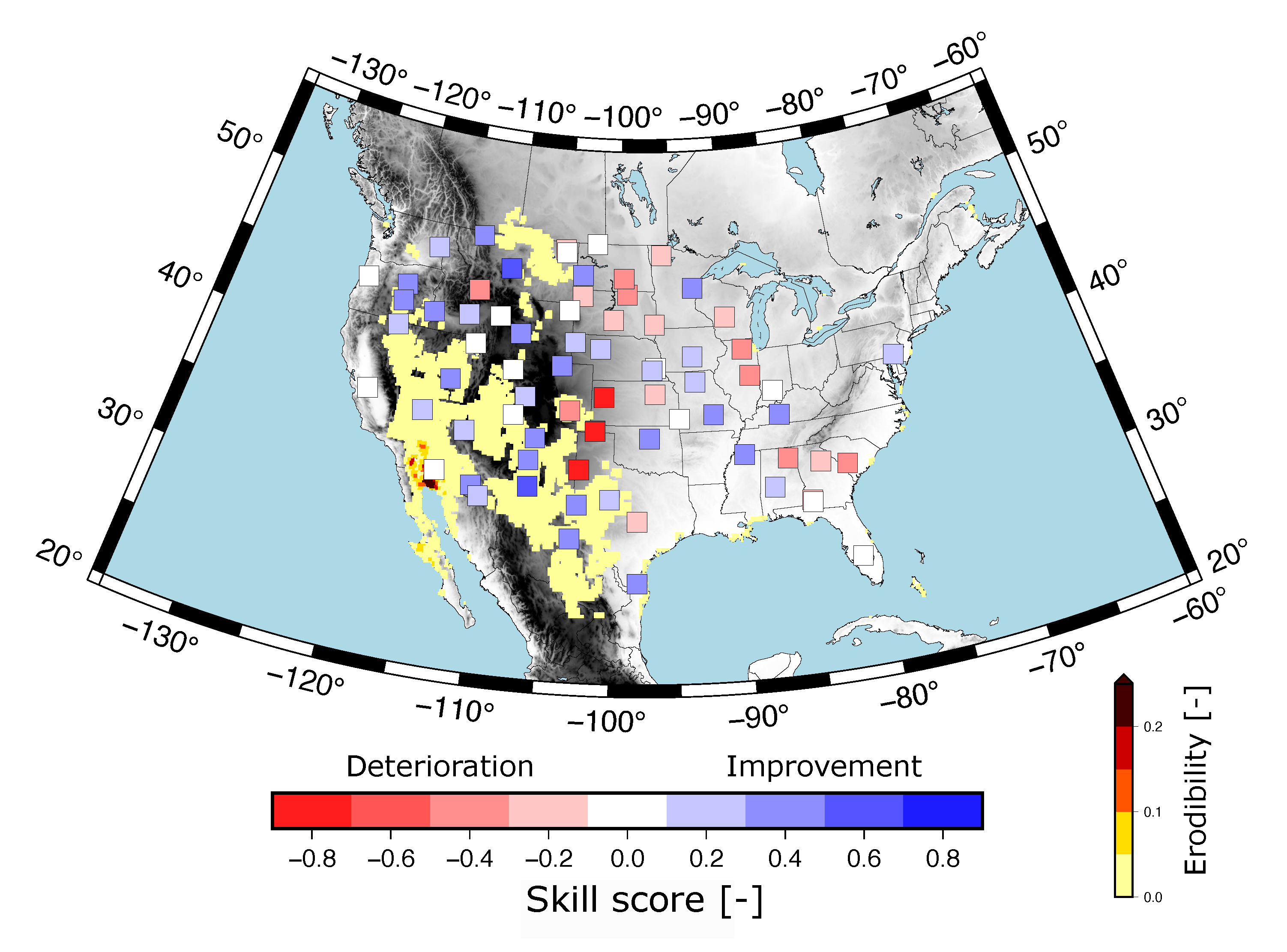
3.1. Added Value of SMAP Soil Moisture
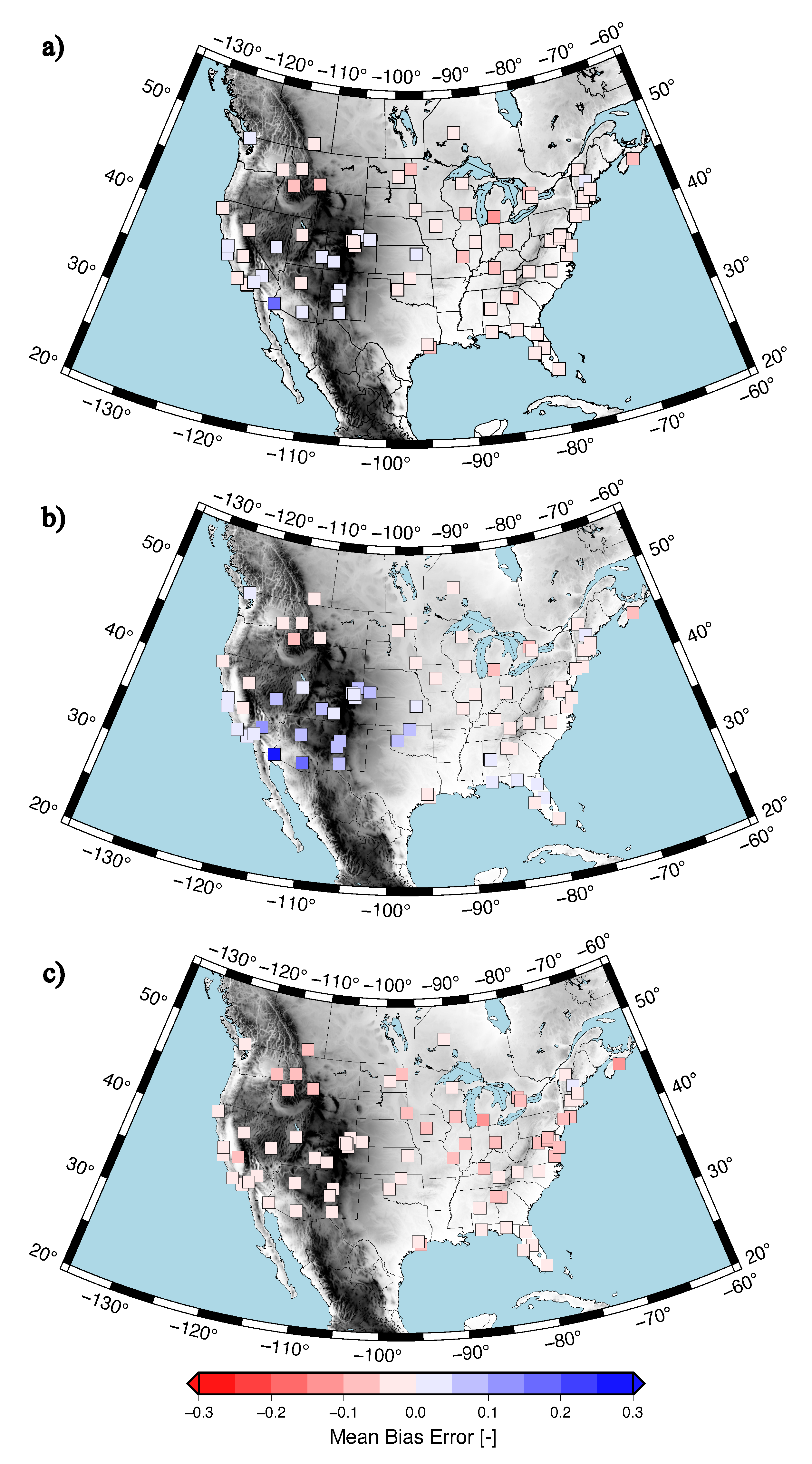
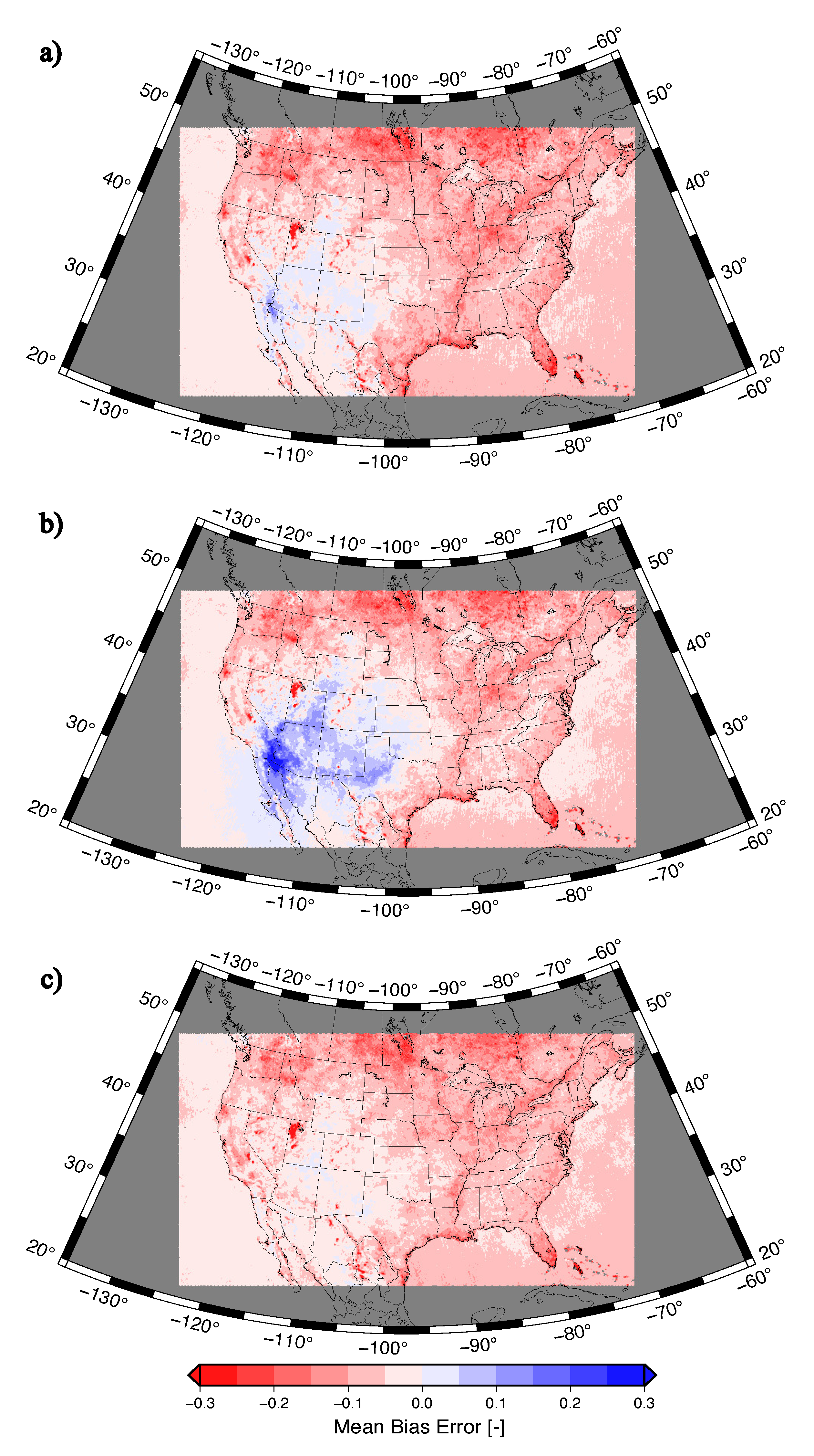
3.2. Near-Surface Meteorological Variables
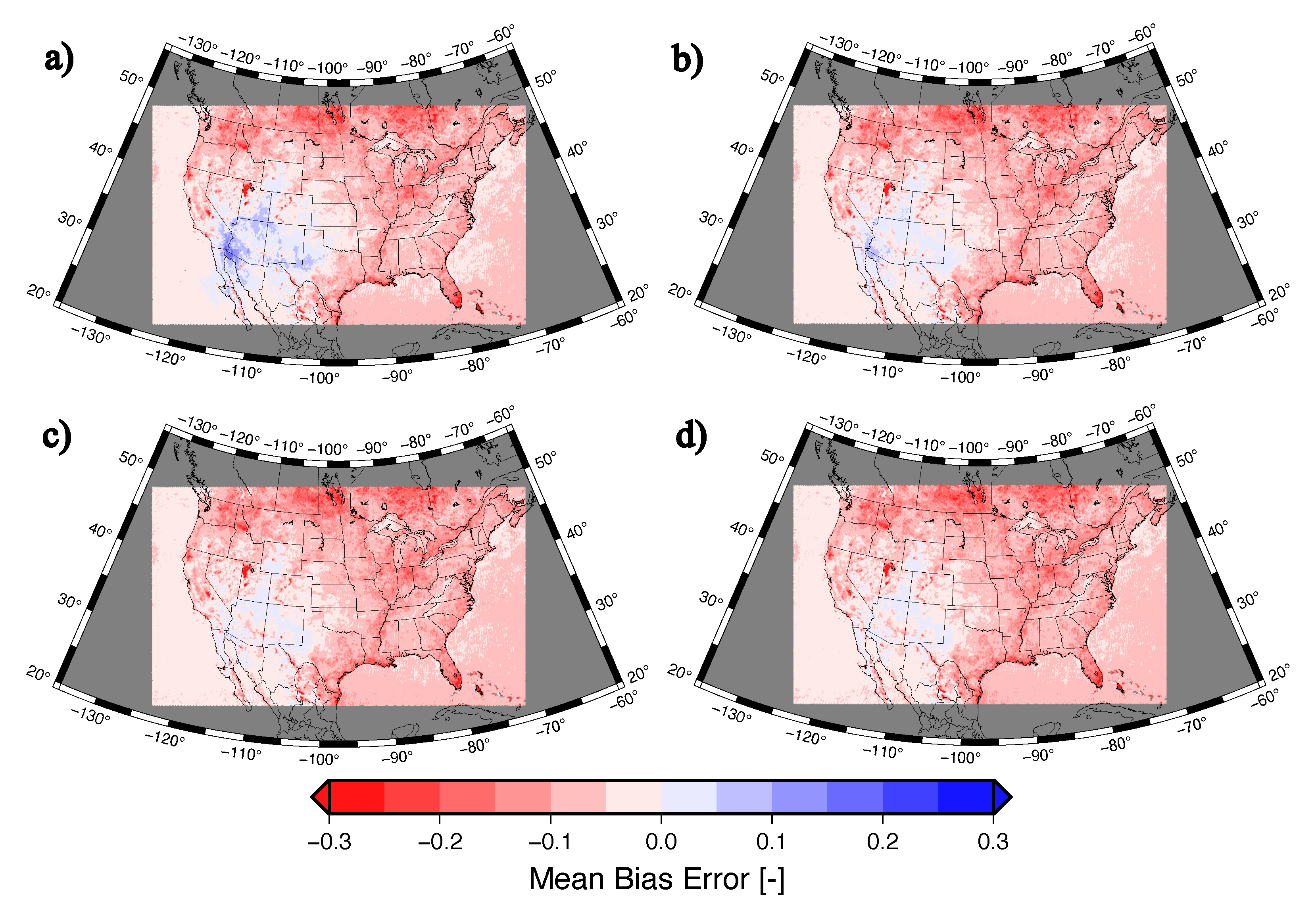
3.3. Aerosol Optical Depth
3.3.1. Effects of the Dust Emission Parameterization
3.3.2. Effects of SMAP Data Insertion
4. Discussion
5. Conclusions
Author Contributions
Funding
Data Availability Statement
Conflicts of Interest
Abbreviations
| AERONET | Aerosol Robotic Network |
| AOD | aerosol optical depth |
| EPA | U.S. Environmental Protection Agency |
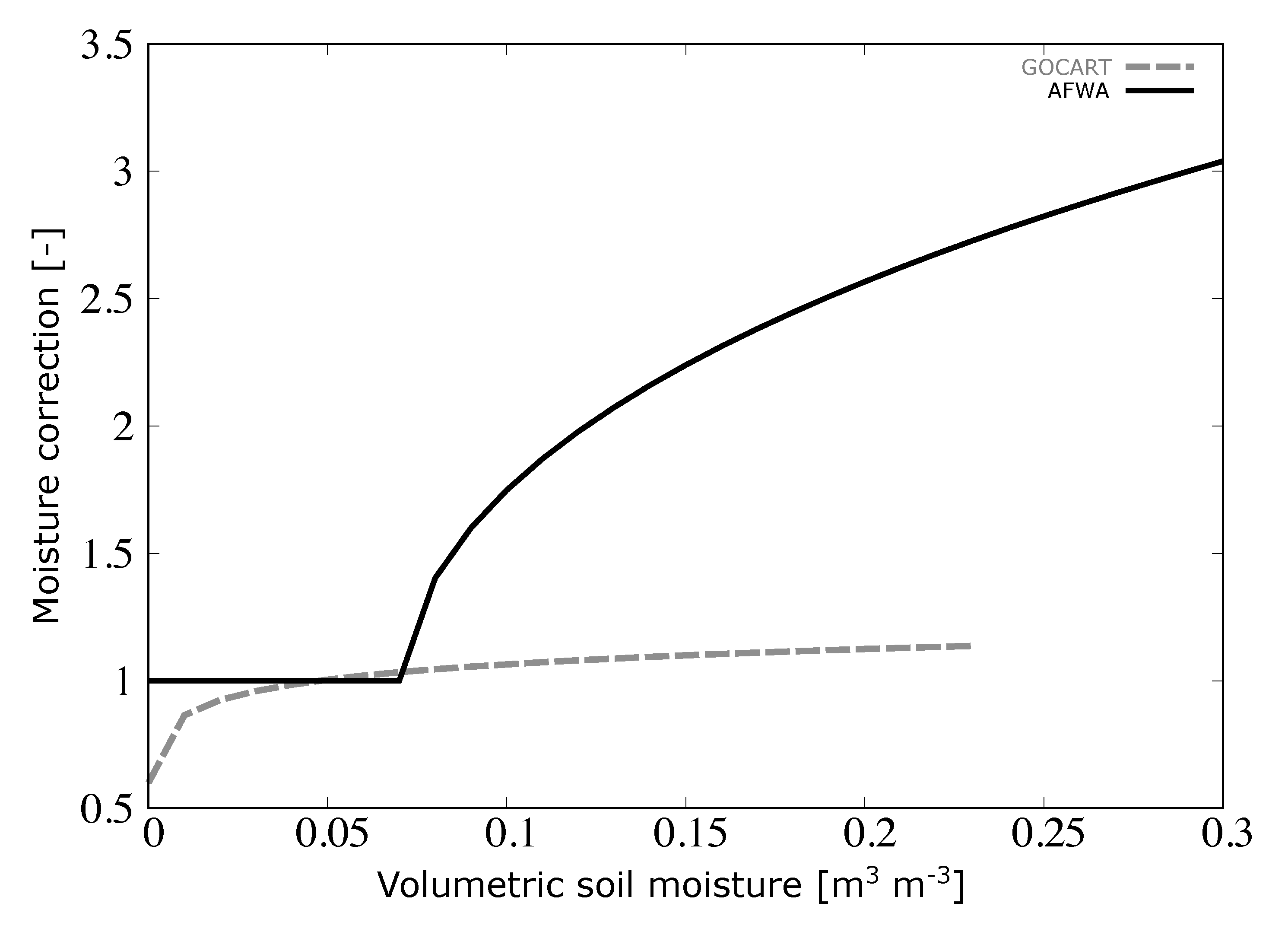
| GOCART | Goddard Chemistry Aerosol Radiation and Transport |
| GOCART-AFWA | GOCART from the Air Force Weather Agency |
| GOCART-AFWA_SMAP | experiment using GOCART-AFWA dust emissions and |
| SMAP retrievals | |
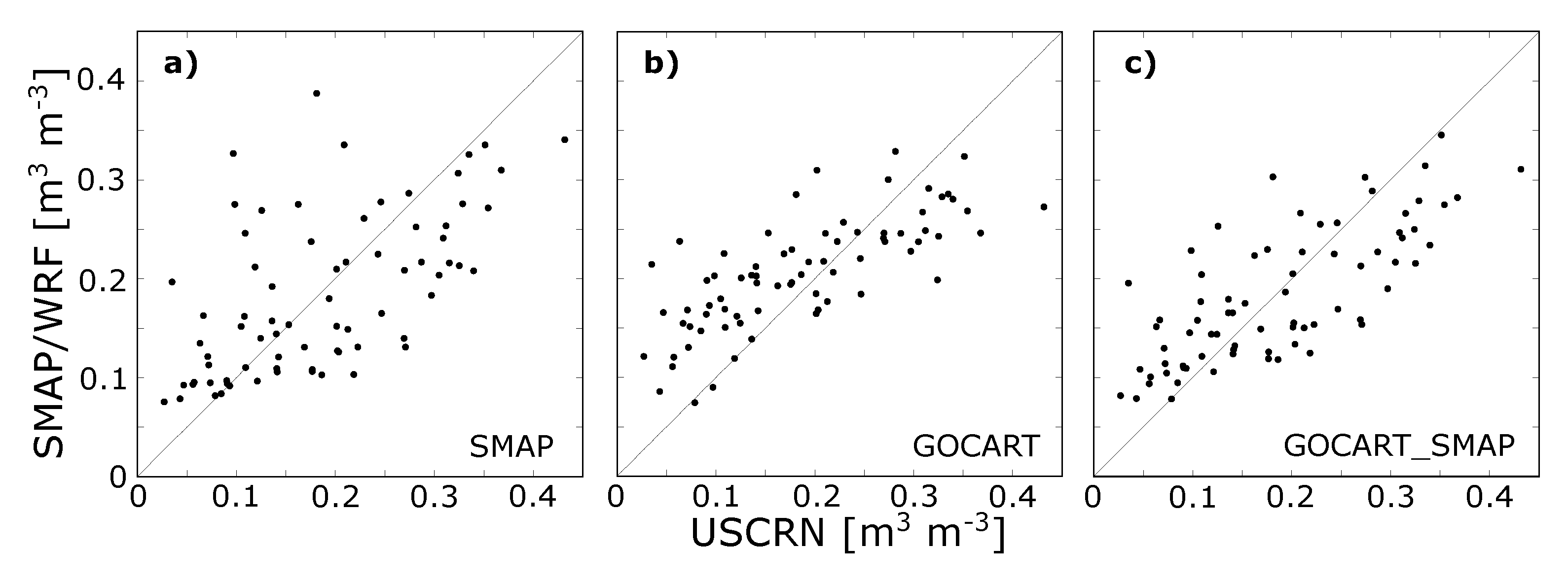
| GOCART_SMAP | experiment using GOCART dust emissions and SMAP retrievals |
| NWP | numerical weather prediction |
| CONUS | contiguous U.S. |
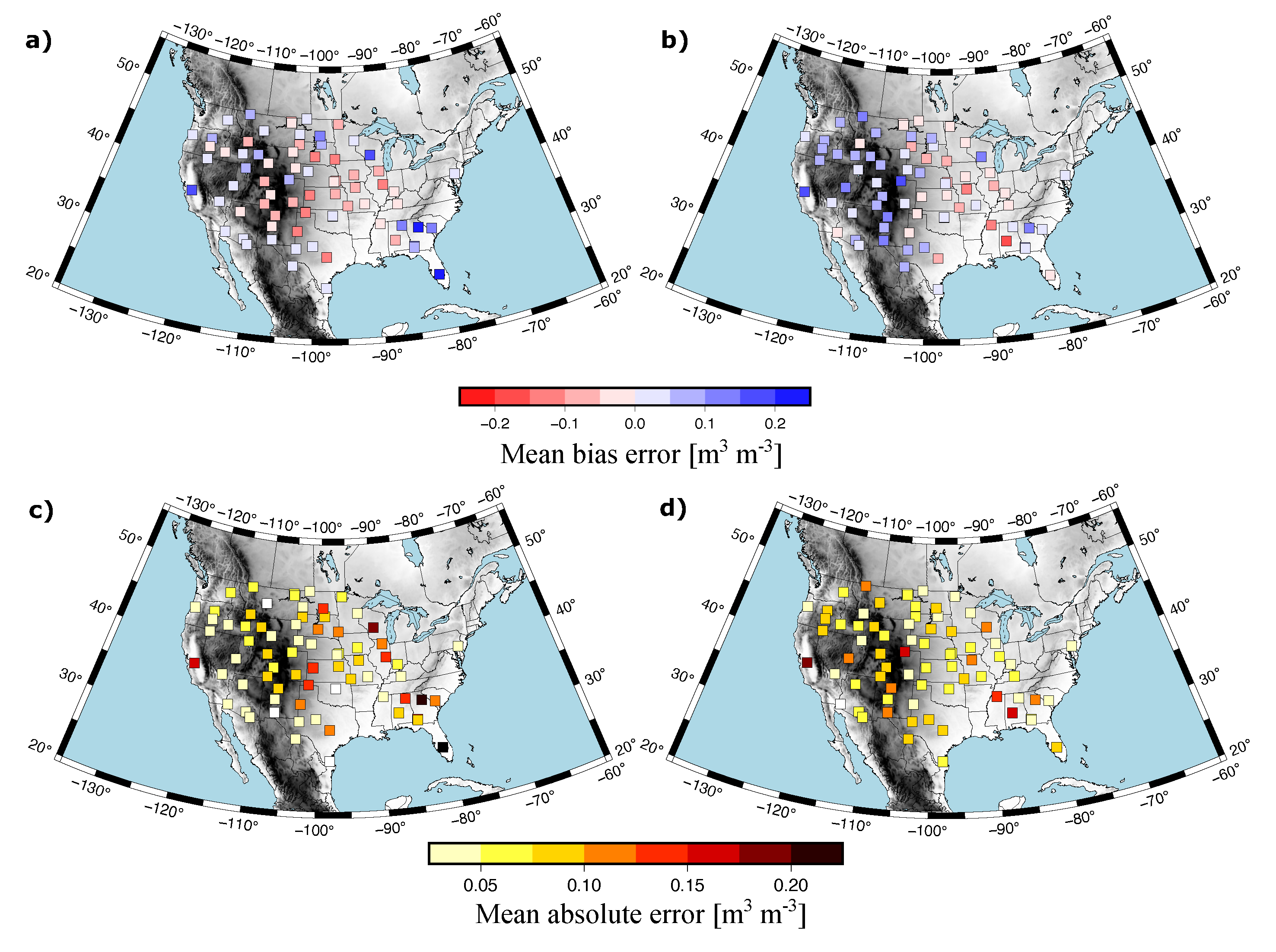
| MAE | mean absolute error |
| MBE | mean bias error |
| MERRA-2 | Modern-Era Retrospective analysis for Research and Applications, |
| Version 2 | |
| METARs | Meteorological Aerodrome Reports |
| MODIS | Moderate Resolution Imaging Spectroradiometer |
| NODUST | experiment without dust emissions |
| NEI | National Emissions Inventory |
| RMSE | root mean square error |
| SMAP | Soil Moisture Active Passive |
| SS | skill score |
| USCRN | U.S. Climate Reference Network |
| EPA | U.S. Environmental Protection Agency |
| WRF | Weather Research and Forecasting |
| WRF-Chem | WRF model coupled with Chemistry |
References
- Bagnold, R. The Physics of Blown Sand and Desert Dunes; Chapmann and Hall: London, UK, 1941; p. 265. [Google Scholar]
- Shao, Y. Physics and Modelling of Wind Erosion; Springer: Berlin/Heidelberg, Germany, 2008; p. 452. [Google Scholar]
- Knippertz, P.; Stuut, J.B.W. Mineral Dust: A Key Player in the Earth System; Springer: Berlin/Heidelberg, Germany, 2014; p. 509. [Google Scholar]
- AlNasser, F.; Chehbouni, A.; Entekhabi, D. Influences of soil moisture and vegetation cover on dust emission using satellite observations. Aeolian Res. 2025, 72, 100961. [Google Scholar] [CrossRef]
- Iversen, J.; Pollack, J.; Greeley, R.; White, B. Saltation threshold on Mars: The effect on interparticle force, surface roughness, and low atmospheric density. Icarus 1976, 29, 381–393. [Google Scholar] [CrossRef]
- Iversen, J.; White, B. Saltation threshold on Earth, Mars, and Venus. Sedimentology 1982, 29, 111–119. [Google Scholar] [CrossRef]
- Marticorena, B.; Bergametti, G. Modeling the atmospheric dust cycle: 1. Design of a soil-dreived dust emission scheme. J. Geophys. Res. 1995, 100, 16415–16430. [Google Scholar] [CrossRef]
- Fécan, F.; Marticorena, B.; Bergametti, G. Parameterization of the increase of the aeolian erosion threshold wind friction velocity due to soil moisture for arid and semi-arid areas. Ann. Geophys. 1999, 17, 149–157. [Google Scholar] [CrossRef]
- Cornelis, W.; Gabriels, D.; Hartmann, R. A parameterisation for the threshold shear velocity to initiate deflation of dry and wet sediment. Geomorphology 2004, 59, 43–51. [Google Scholar] [CrossRef]
- McKenna-Neuman, C.; Nickling, W.G. A theoretical and wind tunnel investigation of the effect of capillarity water on the entrainment of sediment by wind. Can. J. Soil Sci. 1989, 69, 79–96. [Google Scholar] [CrossRef]
- Lin, L.F.; Pu, Z. Improving near-surface short-range weather forecasts using strongly coupled land-atmosphere data assimilation with GSI-EnKF. Mon. Weather Rev. 2021, 148, 2863–2888. [Google Scholar] [CrossRef]
- Entekhabi, D.; Njoku, E.; OŃeill, P.; Kellogg, K.H.; Crow, W.; Edelstein, W.; Entin, J.; Goodman, S.; Jackson, T.; Johnson, J.; et al. The Soil Moisture Active Passive (SMAP) mission. Proc. IEEE 2010, 98, 704–716. [Google Scholar] [CrossRef]
- Lin, L.F.; Pu, Z. Examining the impact of SMAP soil moisture retrievals on short-range weather prediction under weakly and strongly coupled data assimilation with WRF-Noah. Mon. Weather Rev. 2019, 147, 4345–4366. [Google Scholar] [CrossRef]
- Carrera, M.L.; Bilodeau, B.; Bélair, S.; Abrahamowicz, M.; Russell, A.; Wang, X. Assimilation of passive L-band microwave brightness temperatures in the Canadian Land Data Assimilation System: Impacts on short-range warm season numerical weather prediction. J. Hydrol. 2019, 20, 1053–1079. [Google Scholar] [CrossRef]
- Muñoz-Sabater, J.; Lawrence, H.; Albergel, C.; de Rosmay, P.; Isasken, L.; Mesklenburg, S.; Kerr, Y.; Drusch, M. Assimilation of SMOS brightness temperatures in the ECMWF Integrated Forecasting System. Q. J. R. Met. Soc. 2019, 145, 2524–2548. [Google Scholar] [CrossRef]
- Ferguson, C.R.; Agrawal, S.; Beauharnois, M.C.; Xia, G.; Burrows, D.A.; Bosart, L.F. Assimilation of satellite-derived soil moisture for improved forecasts of the Great Plains low-level jet. Mon. Weather Rev. 2021, 148, 4607–4627. [Google Scholar] [CrossRef]
- Grell, G.A.; Peckham, S.E.; Schmitz, R.; McKeen, S.A.; Frost, G.; Skamarock, W.C.; Eder, B. Fully coupled “’online” chemistry within the WRF model. Atmos. Environ. 2005, 39, 6957–6975. [Google Scholar] [CrossRef]
- Fast, J.D.; Gustafson, W.I., Jr.; Easter, R.C.; Zaveri, R.A.; Barnnard, J.C.; Chapman, E.G.; Grell, G.A. Evolution of ozone, particulates, and aerosol direct forcing in an urban area using a new fully-coupled meteorology, chemistry, and aerosol model. J. Geophys. Res. 2006, 111, D21305. [Google Scholar] [CrossRef]
- LeGrand, S.; Polashenski, C.; Letcher, T.; Creighton, G.; Peckham, S.; Cetola, J. The AFWA dust emission scheme for the GOCART aerosol model in WRF-Chem v3.8.1. Geoesci. Model Dev. 2019, 12, 131–166. [Google Scholar] [CrossRef]
- Lee, J.A.; Jiménez, P.A.; Kumar, R.; He, C. Impact of direct insertion of SMAP soil moisture retrievals in WRF-Chem for dust storm events in western U.S. Atmos. Environ. 2024, 321, 120348. [Google Scholar] [CrossRef]
- Chin, M.; Ginoux, P.; Kinne, S.; Torres, O.; Holben, B.N.; Duncan, B.N.; Martin, R.; Logan, J.; Higurashi, A.; Nakajima, T. Tropospheric aerosol optical thickness from the GOCART model and comparisons with satellite and sun photometer measurements. J. Atmos. Sci. 2002, 59, 461–483. [Google Scholar] [CrossRef]
- Colarco, P.; da Silva, A.; Chin, M.; Diehl, T. Online simulations of global aerosol distributions in the NASA GEOS-4 model and comparisons to satellite and ground-based aerosol optical depth. J. Geophys. Res. 2010, 115, D14207. [Google Scholar] [CrossRef]
- Ginoux, P.; Chin, M.; Tegen, I.; Prospero, J.M.; Holben, B.; Dubovik, O.; Lin, S.J. Sources and distributions of dust aerosols simulated with the GOCART model. J. Geophys. Res. 2001, 106, 20255–20273. [Google Scholar] [CrossRef]
- Tang, Y.; Pagowski, M.; Chai, T.; Pan, L.; Lee, P.; Baker, B.; Kumar, R.; Monache, L.D.; Tong, D.; Kim, H.C. A case study of aerosol data assimilation with the Community Multi-scale Air Quality Model over the contiguous United States using 3D-Var and optimal interpolation methods. Geoesci. Model Dev. 2017, 10, 4743–4758. [Google Scholar] [CrossRef]
- Santanello, J.; Lawston, P.; Kumar, S.; Dennis, E. Understanding the impacts of soil moisture initial conditions on NWP in the context of land-atmosphere coupling. J. Hydrometeor. 2019, 20, 793–819. [Google Scholar] [CrossRef]
- Diamond, H.J.; Karl, T.R.; Palecki, M.A.; Baker, C.B.; Bell, J.E.; Leeper, R.D.; Easterling, D.R.; Lawrimore, J.H.; Meyers, T.P.; Helfert, M.R.; et al. U.S. Climate Reference Network after one decade of operations: Status and assessment. Bull. Amer. Met. Soc. 2013, 94, 489–498. [Google Scholar] [CrossRef]
- Holben, B.; Eck, T.; Slutsker, I.; Tanré, D.; Buis, J.; Setzer, A.; Vermote, E.; Reagan, J.; Kaufman, Y.; Nakajima, T.; et al. AERONET—A federated instrument network and data archive for aerosol characterization. Remote Sens. Environ. 1998, 66, 1–16. [Google Scholar] [CrossRef]
- Levy, R.C.; Matto, S.; Munchak, L.A.; Remer, L.A.; Sayer, A.M.; Patadia, F.; Hsu, N.C. The collection 6 MODIS aerosol products over land and ocean. Atmos. Meas. Tech. 2013, 6, 2989–3034. [Google Scholar] [CrossRef]
- Gelaro, R.; McCarty, W.; Suárez, M.J.; Todling, R.; Molod, A.; Takacs, L.; Randles, C.A.; Darmenov, A.; Reichle, R.; Wargan, K.; et al. The modern-era retrospective analysis for research and applications, version 2 (MERRA-2). J. Clim. 2017, 30, 5419–5454. [Google Scholar] [CrossRef]
- Wiedinmyer, C.; Kimura, Y.; McDonald-Buller, E.C.; Emmons, L.E.; Buchholz, R.; Tang, W.; Seto, K.; Joseph, M.; Barsanti, K.; Carlton, A.; et al. The Fire Inventory from NCAR version 2.5: An updated global fire emissions model for climate and chemistry applications. Geoesci. Model Dev. 2023, 16, 3873–3891. [Google Scholar] [CrossRef]
- Freitas, S.; Longo, K.M.; Chatfield, R.; Latham, D.; Dias, M.S.; Andreae, M.; Prins, E.; Santos, J.; Gielow, R.; Carvalho, J., Jr. Including the sub-grid scale plume rise of vegetation fires in low resolution atmospheric transport models. Atm. Chem. Phys. 2007, 7, 3385–3398. [Google Scholar] [CrossRef]
- Gong, S.; Barrie, L.; Blanchet, J.P. Modeling sea-salt aerosols in the atmosphere: 1. Model development. J. Geophys. Res. 1997, 102, 3805–3818. [Google Scholar] [CrossRef]
- Jiménez, P.A.; Dudhia, J.; González-Rouco, J.F.; Navarro, J.; Montávez, J.P.; García-Bustamante, E. A revised scheme for the WRF surface layer formulation. Mon. Weather Rev. 2012, 140, 898–918. [Google Scholar] [CrossRef]
- Nakanishi, M.; Niino, H. Development of an improved turbulence closure model for the atmospheric boundary layer. J. Meteorol. Soc. Jpn. 2009, 87, 895–912. [Google Scholar] [CrossRef]
- Olson, J.B.; Kenyon, J.S.; Djalalova, I.; Bianco, L.; Turner, D.D.; Pichugina, Y.; Choukulkar, A.; Toy, M.D.; Brown, J.M.; Angevine, J.; et al. Improving wind energy forecasting through numerical weather prediction model development. Bull. Amer. Met. Soc. 2019, 100, 2201–2220. [Google Scholar] [CrossRef]
- Iacono, M.J.; Delamere, J.S.; Mlawer, E.J.; Shephard, M.W.; Clough, S.A.; Collins, W.D. Radiative forcing by long-lived greenhouse gases: Calculations with the AER radiative transfer models. J. Geophys. Res. 2008, 113, D13103. [Google Scholar] [CrossRef]
- Thompson, G.; Eidhammer, T. A study of aerosol impacts on clouds and precipitation development in a large winter cyclone. J. Atmos. Sci. 2014, 71, 3636–3658. [Google Scholar] [CrossRef]
- Grell, G.A.; Freitas, S. A scale and aerosol aware stochastic convective parameterization for weather and air quality modeling. Atm. Chem. Phys. 2014, 14, 5233–5250. [Google Scholar] [CrossRef]
- Niu, G.Y.; Yang, Z.L.; Mitchell, K.; Chen, F.; Ek, M.; Barlage, M.; Kumar, A.; Niyogi, K.M.D.; Rosero, E.; Tewari, M.; et al. The community Noah land surface model with multiparameterization options (Noah-MP) 1. Model description and evaluation with local-scale measurements. J. Geophys. Res. 2011, 116, D12109. [Google Scholar] [CrossRef]
- He, C.; Valayamkunnath, P.; Barlage, M.; Chen, F.; Gochis, D.; Cabell, R.; Schneider, T.; Rasmussen, R.; Niu, G.Y.; Yang, Z.L.; et al. The Community Noah-MP Land Surface Modeling System Technical Description Version 5.0; Technical Report TN-575+STR; NCAR: Boulder, CO, USA, 2023. [Google Scholar]
- Yangl, Z.L.; Niu, G.Y.; Mitchell, K.; Chen, F.; Ek, M.; Barlage, M.; Longuevergne, L.; Manning, K.; Niyogi, D.; Tewari, M.; et al. The community Noah land surface model with multiparameterization options (Noah–MP): 2. Evaluation over global river basins. Mon. Weather Rev. 2011, 116, D12110. [Google Scholar]
- Jiménez, P.A.; Dudhia, J.; Thompson, G.; Lee, J.A.; Brummet, T. Improving the cloud initialization in WRF-Solar with enhanced short-range forecasting functionality: The MAD-WRF model. Sol. Energy 2022, 239, 221–233. [Google Scholar] [CrossRef]
- van der Veen, S.H. Improving NWP model cloud forecasts using Meteosat Second-Generation imagery. Mon. Weather Rev. 2012, 141, 1545–1557. [Google Scholar] [CrossRef]
- Xu, J.; Shu, H. Assimilating MODIS-based albedo and snow coverfraction into the Common Land Model to improve snow depth simulation with direct insertion and deterministic ensemble Kalman filter methods. J. Geophys. Res. 2014, 119, 10684–10701. [Google Scholar] [CrossRef]
- Zidikheri, M.J.; Lucas, C. Improving ensemble volcanic ash forecasts by direct insertion of satellite data and ensemble filtering. Atmosphere 2021, 12, 1215. [Google Scholar] [CrossRef]
- Computational and Information Systems Laboratory. Cheyenne: HPE/SGI ICE XA System (NCAR Community Computing); National Center for Atmospheric Research: Boulder, CO, USA, 2021. [Google Scholar] [CrossRef]

| Experiment Name | Emissions | SMAP | Emissions Factor |
|---|---|---|---|
| Exp1 (GOCART) | GOCART | No | - |
| Exp2 (GOCART_SMAP) | GOCART | Yes | - |
| Exp3 (GOCART-AFWA) | GOCART-AFWA | No | 1.0 |
| Exp4 (GOCART-AFWA_SMAP) | GOCART-AFWA | Yes | 1.0 |
| Exp5 | GOCART-AFWA | No | 0.5 |
| Exp6 | GOCART-AFWA | Yes | 0.5 |
| Exp7 | GOCART-AFWA | No | 0.25 |
| Exp8 | GOCART-AFWA | Yes | 0.25 |
| Exp9 | GOCART-AFWA | No | 0.1 |
| Exp10 | GOCART-AFWA | Yes | 0.1 |
| Exp11 | GOCART-AFWA | No | 0.05 |
| Exp12 | GOCART-AFWA | Yes | 0.05 |
| Exp13 (NODUST) | - | Yes | - |
| Experiment | MBE | MAE | RMSE | Corr |
|---|---|---|---|---|
| SMAP | −0.5 | 7.2 | 9.2 | 0.65 |
| GOCART | 2.0 | 7.1 | 8.9 | 0.68 |
| GOCART_SMAP | −0.5 | 6.5 | 8.3 | 0.71 |
| Region | MBE | MAE | RMSE | Corr |
|---|---|---|---|---|
| R1: New England | 0.05/8 | 0.60/26 | 0.85/38 | 0.82/0.80 |
| R2: New York, New Jersey | 0.02/2 | 0.68/26 | 0.85/37 | 0.85/0.83 |
| R3: Mid-Atlantic | 0.78/3 | 0.85/20 | 1.01/28 | 0.89/0.90 |
| R4: Southeast | 0.74/2 | 0.78/16 | 0.90/22 | 0.88/0.91 |
| R5: Upper Midwest/Great Lakes | 0.53/3 | 0.64/12 | 0.76/16 | 0.93/0.96 |
| R6: South Central | 0.51/6 | 0.66/17 | 0.80/23 | 0.89/0.86 |
| R7: Midwest | −0.02/5 | 0.60/16 | 0.76/23 | 0.90/0.92 |
| R8: Mountains and Plains | 0.01/6 | 0.44/15 | 0.56/20 | 0.90/0.84 |
| R9: Pacific Southwest | 0.28/10 | 0.62/19 | 0.75/23 | 0.84/0.83 |
| R10: Pacific Northwest | 0.24/9 | 0.51/24 | 0.63/29 | 0.84/0.72 |
Disclaimer/Publisher’s Note: The statements, opinions and data contained in all publications are solely those of the individual author(s) and contributor(s) and not of MDPI and/or the editor(s). MDPI and/or the editor(s) disclaim responsibility for any injury to people or property resulting from any ideas, methods, instructions or products referred to in the content. |
© 2025 by the authors. Licensee MDPI, Basel, Switzerland. This article is an open access article distributed under the terms and conditions of the Creative Commons Attribution (CC BY) license (https://creativecommons.org/licenses/by/4.0/).
Share and Cite
Jiménez y Muñoz, P.A.; Kumar, R.; He, C.; Lee, J.A. Revisiting the Role of SMAP Soil Moisture Retrievals in WRF-Chem Dust Emission Simulations over the Western U.S. Remote Sens. 2025, 17, 1345. https://doi.org/10.3390/rs17081345
Jiménez y Muñoz PA, Kumar R, He C, Lee JA. Revisiting the Role of SMAP Soil Moisture Retrievals in WRF-Chem Dust Emission Simulations over the Western U.S. Remote Sensing. 2025; 17(8):1345. https://doi.org/10.3390/rs17081345
Chicago/Turabian StyleJiménez y Muñoz, Pedro A., Rajesh Kumar, Cenlin He, and Jared A. Lee. 2025. "Revisiting the Role of SMAP Soil Moisture Retrievals in WRF-Chem Dust Emission Simulations over the Western U.S." Remote Sensing 17, no. 8: 1345. https://doi.org/10.3390/rs17081345
APA StyleJiménez y Muñoz, P. A., Kumar, R., He, C., & Lee, J. A. (2025). Revisiting the Role of SMAP Soil Moisture Retrievals in WRF-Chem Dust Emission Simulations over the Western U.S. Remote Sensing, 17(8), 1345. https://doi.org/10.3390/rs17081345