Abstract
Near-global Digital Elevation Model (DEM) products generated through space-based radar techniques have become a basic data source for a variety range of applications. However, these DEM products often contain typical errors such as vegetation bias and topography-related errors, which impede their practical utility. Despite the development of numerous correction methods based on mathematical fitting and artificial neural networks over recent decades, reliably correcting large-scale spaceborne radar-derived DEMs remains an open challenge due to issues like underfitting or overfitting. This paper introduces a novel framework called Feature-Reinforced Ensemble Learning (FREEL) designed specifically for correcting space-based radar-derived DEMs. Within this FREEL framework, a feature derivation module and a feature reinforcement module are integrated to enhance the original input features. Subsequently, an adaptive weighting variant of the DeepForest algorithm is proposed to emphasize critical features and improve training robustness, even with limited training data. The Shuttle Radar Topographic Mission (SRTM) DEMs of Hunan Province, China, characterized by diverse surface terrain and vegetation coverage, were selected to evaluate the FREEL framework. The results indicate that the accuracy of the SRTM DEM corrected using the FREEL framework improved by 40%, surpassing several mathematical fitting and machine learning baseline algorithms by an average of 45% and 23%, respectively. This method provides a more robust solution for correcting near-global space-based radar-derived DEM products.
1. Introduction
Digital Elevation Models (DEMs) have found extensive application in various fields, including topography, hydrology, and ecology. The accuracy of DEM products is critical for these applications. Traditionally, high-precision DEMs have been generated using geodetic surveying techniques such as leveling and GNSS, as well as ground-based or airborne Light Detection and Ranging (lidar). However, due to the high costs associated with these methods, such high-quality DEM products are available only for limited areas or specific local regions. For generating DEMs with near-global or global coverage, space-based remote sensing techniques are preferred [1,2], owing to their advantages of broad coverage, low cost, and higher spatial resolution compared to traditional methods. For instance, the Shuttle Radar Topography Mission (SRTM) produced DEMs covering 80% of the Earth’s land surface (from 60°N to 57°S) using spaceborne imaging radar sensors between 11 and 22 February 2000 [3]. These near-global SRTM DEMs have become one of the most widely used DEM products for scientific applications. Nonetheless, significant errors such as vegetation bias, topography-related errors, and global errors often exist in space-based radar-derived DEMs [4]. These errors, largely attributed to the vegetation penetration capability of radar microwave and the unique imaging mode, significantly limit the practical applications of space-based radar-derived DEMs [5].
In recent decades, numerous methodologies have been developed for the correction of space-based radar-derived DEMs. These methodologies predominantly involve fitting and subsequently mitigating DEM errors through user-defined mathematical functions or machine learning algorithms. This process is facilitated by accurate reference elevation datasets obtained from ground-based geodetic surveying techniques (e.g., leveling and GNSS), airborne lidar, and satellite-based laser altimeters [5,6,7,8]. For the mathematical fitting algorithms, in addition to auxiliary reference elevation datasets, the effectiveness of DEM correction largely hinges on the capability of the fitting algorithms to accurately describe the error patterns inherent in space-based DEM products. To date, it remains challenging to manually define a suitable mathematical function (e.g., linear or topography-related nonlinear functions) that can perfectly capture the complex error patterns of near-global DEMs, such as those derived from SRTM. In contrast to user-defined mathematical fitting, machine learning algorithms possess a robust ability to perform complex nonlinear fitting without the need for manual function definition. Consequently, several machine learning algorithms, including artificial neural network (ANN) [9], deep neural network (DNN) [10], and random forests [11,12], have been extensively employed for correcting space-based radar-derived DEMs.
Despite significant efforts dedicated to the correction of space-based radar-derived DEMs, reliably correcting near-global DEMs remains an open challenge. This is primarily due to inherent limitations in current machine learning algorithms. For example, ANN and DNN models necessitate extensive training datasets, with their performance critically dependent on the empirical tuning of numerous hyperparameters [13,14]. Consequently, considerable resources are required for data collection and hyperparameter optimization. Moreover, popular ensemble learning models such as random forests are susceptible to overfitting, particularly when dealing with datasets that contain substantial noise or outliers [15].
Here, we introduce a novel framework named Feature-REinforced Ensemble Learning (FREEL) designed for the correction of space-based radar-derived DEMs. The FREEL framework comprises three core modules: the Feature Derivation Block (FDB), the Feature Reinforcement Block (FRB), and an innovative DeepForest ensemble learning module. Specifically, the FDB integrates multiple feature derivation layers along with a recursive feature elimination layer to capture the interactions and dependencies among the original input features [16,17]. The FRB incorporates depth-wise convolutional layers, pooling layers, and attention mechanisms, aiming to extract spatially abstract and complex representations that surpass the capabilities of the FDB. By leveraging both the FDB and FRB, the FREEL framework can derive more comprehensive features related to DEM errors from the initial input data, thereby enhancing the accuracy of the learning process. Subsequently, we propose a new DeepForest ensemble learning module called AdDeepForest for network training. The AdDeepForest module exhibits reduced sensitivity to hyperparameter tuning and maintains performance even with small-scale training datasets. Consequently, it mitigates the dependency on extensive hyperparameter tuning required by traditional ANN and DNN algorithms and potentially alleviates the overfitting risk associated with a single random forest. These advantages contribute to the overall robustness of the FREEL framework in correcting space-based radar-derived DEMs.
The remainder of this paper is organized as follows. Section 2 outlines the methodology of the proposed FREEL framework for space-based radar-derived DEM correction. Section 3 shows the experimental setup and results, wherein the FREEL framework was employed to correct SRTM DEM products over Hunan Province, China, using reference elevation data obtained from GPS Continuously Operating Reference Station (CORS) rovers and the Ice, Cloud, and Land Elevation Satellite (ICESat-2) sensor. Section 4 provides a detailed discussion on the performance and advantages of the FREEL framework, while Section 5 offers concluding remarks.
2. Methodology
The errors of space-based radar-derived DEM products are mainly related to land cover, topography, locations, and so forth [4,18,19,20]. Therefore, we selected nine indicators, i.e., latitude, longitude, elevation, slope, aspect, vegetation coverage, land cover types, canopy height, and leaf area index (LAI), to roughly describe these related factors. The datasets of the selected nine indicators were serviced to be the originally input features of the proposed FREEL framework and further used to correct space-based radar-derived DEMs.
2.1. Construction of the FREEL Framework
2.1.1. The FDB Module for Feature Derivation
The FDB module comprises three key components: a high-order derivation layer, a polynomial derivation layer, and a recursive feature elimination layer (see Figure 1a). Within this architecture, the high-order derivation layer identifies complex nonlinear relationships in the input feature space, producing advanced high-order features to optimize training efficiency for the FREEL framework [21,22]. In the current study, the original nine input features are computationally expanded into a third-order dimensional space, resulting in a total of 27 features. This enhancement includes the base nine features, nine second-order interactions, and nine third-order nonlinear combinations derived from the original feature set.
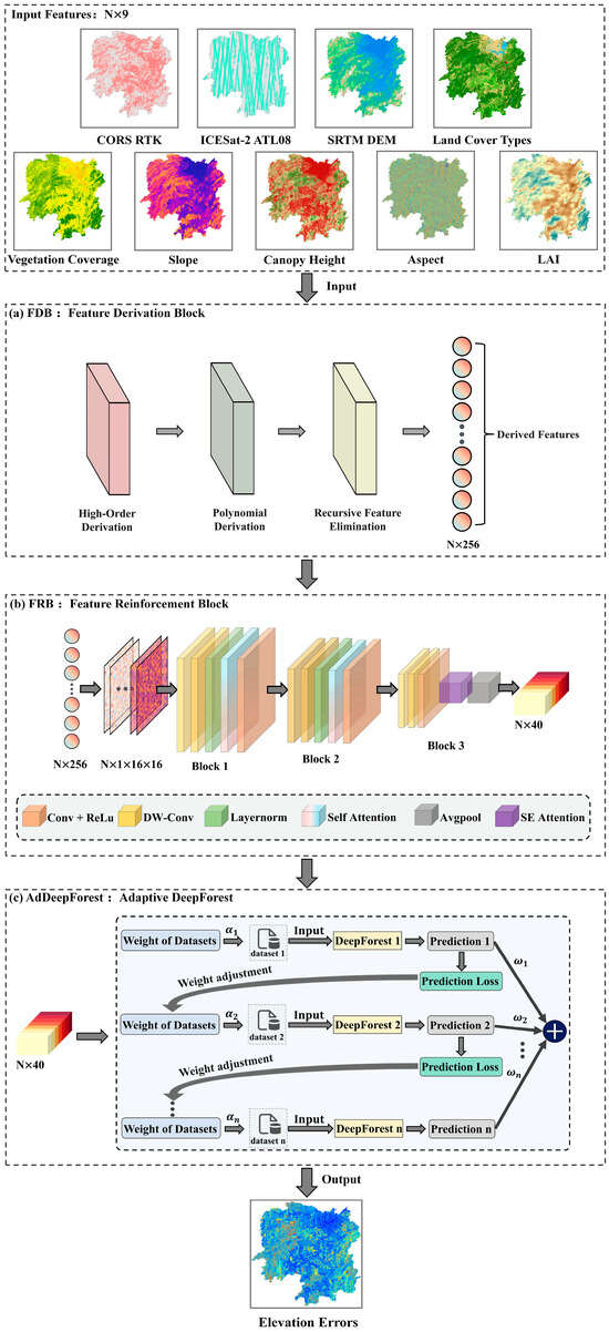
Figure 1.
Flowchart of space-based radar-derived DEM correction using the FREEL framework. (a–c) show the structures of the FDB, FRB, and the AdDeepForest modules in the FREEEL framework.
It is noteworthy that while the high-order derivation layer exclusively captures high-dimensional self-information of individual input features, it inadequately models inter-feature interactions. To address this limitation, we incorporate a novel polynomial derivation layer within the FREEL framework, designed to characterize interactive dependencies through polynomial combinations [23]. In the current implementation, cubic polynomial combinations are strategically employed to balance the trade-off between interaction modeling efficacy and computational efficiency. Specifically, triadic feature subsets are randomly sampled from the 27 high-order-derived features to generate new combinatorial representations via cubic polynomial operations. This approach expands the feature space dimensionality from an initial set of 9 to 2925 synthesized features.
The polynomial derivation layer generates 2925 features that may contain redundant elements and extreme values, potentially exacerbating learning complexity [24,25]. To mitigate this, we employ a Support Vector Machine (SVM)-based recursive feature elimination (RFE) mechanism that systematically reduces feature dimensionality while preserving discriminative power. Through iterative SVM training cycles, feature weights are dynamically updated to quantify importance metrics. The algorithm retains features with high weight coefficients and eliminates those with minimal weights in each elimination phase. This differential selection process iterates until converging to the predetermined optimal dimensionality of 256 features, achieving an equilibrium between feature representation capability and computational tractability (Figure 1b) [26].
2.1.2. The FRB Module for Feature Reinforcement
While the Feature Derivation Block (FDB) effectively expands feature representations through high-order dimensional properties and interaction dependencies, it inherently neglects to account for spatial patterns correlated with DEM errors. Theoretical foundations [27] strongly advocate for the integration of spatial features to enhance model training efficacy. To bridge this critical gap, we propose a novel Feature Reinforcement Block (FRB) module specifically engineered to augment input features for DEM error correction. The FRB synergistically combines (1) the superior capability of convolutional neural networks (CNNs) in extracting deep hierarchical patterns from high-dimensional data [28,29] and (2) the computationally efficient global context modeling enabled by Transformer-based self-attention mechanisms [30,31].
More specifically, as shown in Figure 1b, the one-dimensional feature sets are initially transformed into a two-dimensional feature map of to facilitate computation by the convolutional layers, where denotes the number of channels, and represents the height and width of the transformed two-dimensional feature map. In Block 1 of Figure 1b, the two-dimensional feature map is firstly processed by two layers of depth-wise convolution to enrich the feature representation by expanding the original channel number from 1 to 16. The depth-wise convolution is able to reduce the number of parameters and computational complexity while maintaining model performance, compared with traditional convolution networks [32]. However, the convolutional layers in the depth-wise convolution network can well capture the local spatial information of the feature maps but usually fail to capture global information whose spatial scale exceeds the window size of the convolution kernel.
The multi-head self-attention mechanism demonstrates exceptional capacity for capturing intricate global interdependencies among high-dimensional features [30]. Capitalizing on this inherent capability, we employ this mechanism to process the feature maps produced by dual depth-wise convolutional layers, enabling the comprehensive extraction of cross-regional contextual information. A critical preprocessing step involves implementing layer normalization prior to the self-attention computation, which substantially improves training stability and convergence properties during the feature refinement phase. Following the extraction of global feature information, the feature map is processed again through a standard convolutional layer and a ReLu activation function for effectively reducing the width and height by half.
To enable multi-scale feature learning, Block 1 outputs undergo progressive refinement through Block 2 (architecturally identical to Block 1). The resulting hierarchical features from Block 2 are then processed by Block 3, which implements two critical operations: (1) a Squeeze-and-Excitation (SE) attention mechanism for adaptive channel-wise feature enhancement and (2) global average pooling for dimensionality reduction to a 1D feature vector (Figure 2). This 40-element vector synthesizes multi-scale spatial information through global–local feature interactions, providing optimized input for the AdDeepForest-based DEM correction while ensuring computational efficiency.
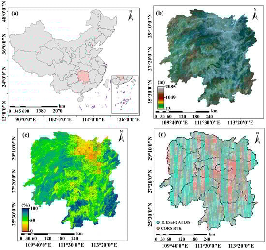
Figure 2.
(a): Location of Hunan Province, China; (b,c) terrain and vegetation coverage of Hunan Province; and (d) spatial distribution of the collected CORS RTK and ICESat-2 ATL08 elevation observations.
2.1.3. AdDeepForest for DEM Correction
Originally proposed by Zhou and Feng (2019) [33], the DeepForest algorithm (DF) represents a multi-layered cascade forest ensemble framework. Diverging from conventional deep neural networks (DNNs) that employ differentiable nonlinear transformations through artificial neurons, DF’s architectural core resides in its layered integration of non-differentiable random forest units. This distinctive architecture confers two principal advantages: (1) enhanced robustness to hyperparameter sensitivity and (2) reliable performance under small-sample training regimes where DNNs typically suffer from severe overfitting [33]. The multi-tiered ensemble design systematically mitigates overfitting risks inherent to individual decision trees through diversified forest aggregation. Nevertheless, DF’s current implementation adopts uniform weighting across all constituent forests during prediction integration. This egalitarian approach overlooks critical performance heterogeneity among submodels, particularly variations in (a) individual forest prediction fidelity and (b) feature subspace importance. Such oversight potentially undermines the algorithm’s capacity to leverage model diversity for enhanced robustness, as substantiated by recent theoretical analyses [34].
To overcome this issue, we proposed a variant of DeepForest (referred to as AdDeepForest), where an Adaptive Boost (AdaBoost) algorithm [35] is incorporated into the DeepForest algorithm for adaptive weighting by considering fitting qualities and feature importance. As depicted in Figure 1c, the AdDeepForest algorithm predicts the elevation error based on the FRB-reinforced features and refines DEM accuracy by subtracting the predicted error from the original DEM. Let be the current datasets with () being the FRB-generated features and being the DEM elevation error at the ith training sample. We firstly aggregate multiple DeepForests into a single reinforced DeepForest, termed AdDeepForest, based on the AdaBoost objective function .
where denotes the number of DeepForests, represents the DeepForest prediction models, and denotes the weights for each DeepForest. The initial weight of each training sample is assigned by . A DeepForest is then trained on the weighted dataset, and the total current prediction loss is computed by Equation (2).
where is the number of all the training samples, and denotes the prediction loss (mean square error, MSE) of the DeepForest at each training sample, which is calculated by
with being the true elevation error and being the predicted elevation error. The weight of the current DeepForest is then estimated based on the prediction loss, i.e.,
In Equation (6), the parameter of is iteratively updated by
In doing so, the weights of those training samples with large prediction losses will be increased, whereas the weights of those samples with small prediction losses will be decreased. As a consequence, the training model will pay more attention to those training samples that are difficult to predict precisely, increasing the robustness of the prediction. After iterating the process T times, the predictions from all DeepForests are aggregated through weighted voting to obtain the prediction function of the reinforced DeepForest, which ultimately outputs the predicted elevation error.
The flowchart of the FREEL framework for space-based radar-derived DEM correction is shown in Figure 1.
3. Experiments and Results
3.1. Study Areas
Hunan Province, which is located in the central southern part of China (see Figure 2a), was selected to test the performance of DEM correction using the proposed FRELL framework. The area of Hunan Province is about 285,100 km2, where the elevation varies from 13 m to 2085 m, and the terrain slope changes from 0° to 68° (see Figure 2b). In addition, three typical types of terrain (i.e., plain, mountain, and hill) are contained in Hunan Province, and the area of mountain and hill occupies around 80% of the surface. The vegetation in Hunan Province is varied (see Figure 2c), with an average vegetation coverage of 65.5%. This allows us to test DEM correction using the proposed FREEL framework in different types of terrain and different vegetation coverage.
3.2. Datasets
3.2.1. SRTM DEM
The Shuttle Radar Topography Mission (SRTM) was a radar topography-measuring mission conducted by the National Aeronautics and Space Administration (NASA) in 2000. It generated DEMs over nearly 80% of Earth’s land surfaces (from 60°N to 56°S) using the Interferometric Synthetic Aperture Radar (InSAR) technique [36]. In 2003, the first version of the SRTM DEM products (Version 1) was released. The “finished” SRTM DEM (i.e., Version 2) was then released, where substantial editing was devoted by the National Geospatial Intelligence Agency, exhibiting well-defined water bodies and coastlines and removing spikes and outliers. The Shuttle Radar Topography Mission Digital Elevation Model (SRTM DEM) Version 3 (SRTM v3), publicly released in 2013, resolved persistent data voids present in Version 2 through advanced gap-filling algorithms while maintaining its native 3-arc-second (~90 m) global resolution. Subsequent advancements include the following: (1) the 2018 global release of 1-arc-second (30 m) resolution void-filled SRTM products, and (2) the 2020 deployment of NASADEM, which implemented critical enhancements, such as radar signal reprocessing and ICESat-derived vertical datum calibration. For our Hunan Province case study (Figure 2a), we deliberately selected SRTM v3 over NASADEM to preserve the original error characteristics of the SRTM’s C-band radar measurements—a critical factor given NASADEM’s elevation adjustments fundamentally alter the error distribution patterns crucial for our correction model validation.
3.2.2. Auxiliary Observations of Reference Elevation
This study employs two geodetic-grade elevation datasets as reference benchmarks for SRTM DEM correction. The primary reference dataset comprises photon-derived elevation measurements acquired by the Advanced Topographic Laser Altimeter System (ATLAS) aboard NASA’s Ice, Cloud, and Land Elevation Satellite-2 (ICESat-2). This spaceborne photon-counting lidar system achieves centimeter-level vertical accuracy through precise photon time-of-flight measurements, establishing it as an optimal reference source for DEM quality assessment and error characterization [35]. The mean bias and root mean square error (RMSE) of the ATL08 terrain products produced from the ATLAS datasets is usually below 1 m and in the range from 0.2 m to 2 m [37,38,39]. Such an accuracy level is much higher than the SRTM DEM products (at a level of 10~20 m) [18]. In this study, 529,800 ICESat-2 observations over Hunan Province were collected from the strong nighttime beam of the ATL08 dataset in the period between January 2019 and December 2022. The footprints of the collected ATL08 elevations are marked by cyan circles in Figure 2d.
The other type of high-quality auxiliary elevations were collected from the Hunan CORS network, where 130 base stations are composed and the signals of GPS/GLONASS/GALELEO/BDS satellites are included in the Hunan CORS network [40]. The Hunan CORS network enables to offer elevation observations with a centimeter-level accuracy in both vertical and horizontal dimensions using real-time kinematic (RTK) positioning techniques [41,42]. In this study, we collected 4,830,711 elevation observations from the RTK trajectories in the Hunan CORS network to serve as references in order to increase the samples and improve the spatial distribution of the reference elevation for SRTM DEM correction. The locations of the collected CORS elevation observations are marked by light red circles in Figure 2d.
3.2.3. Datasets of Input Features
In this study, nine parameters relating to SRTM DEM errors, i.e., latitude, longitude, elevation, slope, aspect, vegetation coverage, land cover types, canopy height, and LAI, were selected to be the originally input features [5,6,43]. Of these, the first five features (i.e., latitude, longitude, elevation, slope, and aspect) were obtained from the original SRTM DEM products. The feature of vegetation coverage was collected from the normalized difference vegetation index (NDVI) products provided by NASA. Note that the NASA NDVI product with a resolution of 250 m was oversampled to 30 m using the algorithm presented by [44] in order to meet the resolution of the SRTM DEM products. The feature of land cover type was collected from the Globalland30 datasets of 2020 (https://www.un-spider.org/links-and-resources/data-sources/land-cover-map-globeland-30-ngcc, accessed on 25 March 2025), with a classification accuracy over 80% [45,46]. The features of canopy height and LAI were yielded from the open-access datasets of [47,48].
3.3. SRTM DEM Correction Using the FREEL Framework
The FREEL framework corrects SRTM DEM errors in Hunan Province through the integration of reference elevation samples (CORS RTK measurements) and nine optimized feature datasets. Figure 2d reveals concentrated sampling in flat terrain and low-relief hills, potentially introducing geographical bias. To mitigate this, we employ spatial stratification to subsample clustered observations, ensuring geographical representativeness. The processed dataset undergoes stratified partitioning, 70% (3850 samples) for model training and 30% (1650 samples) for independent validation, maintaining proportional distribution across terrain types as detailed in Figure 3. Then, the FREEL framework was utilized for SRTM DEM correction with the assistance of the ICESat-2 and CORS elevation references. The FDB module was firstly used to expand the originally input 9 features to 256 by setting the feature derivation of third-order and cubic polynomials and setting the threshold of recursive feature elimination to 256. The FDB-derived 256 features were further processed by the FRB module to extract 40 abstract and complex features. In the FRB, all the convolutional kernels had a size of , the number of heads for the self-attention mechanism was 6, and the compression ratio for the SE Attention was 4. The 40 FRB-extracted features were than input into the AdDeepForest algorithm to train and predict the elevation errors of the SRTM DEM products. In the AdDeepForest framework, each DeepForest consisted of 15 cascading layers, and each layer contained five random forests. The FREEL algorithm was trained over 300 epochs. Finally, the FREEL-corrected DEM products were obtained by subtracting the FREEL-predicted elevation errors from the original SRTM DEM products.
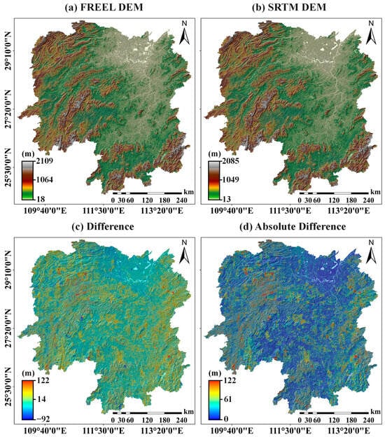
Figure 3.
Comparison between the FREEL-corrected SRTM DEM (a) and the original SRTM DEM (b) in Hunan Province. (c,d) illustrate the differences and the absolute differences between the original and FREEL-corrected SRTM DEM, respectively.
Figure 3a–c, respectively, present (1) the original SRTM DEM, (2) its FREEL-corrected counterpart, and (3) the vertical discrepancy map across Hunan Province. The correction process reveals substantial vertical adjustments ranging from −92 m (subsidence) to +122 m (uplift), with spatial error patterns demonstrating strong terrain dependency. Notably, positive corrections (SRTM overestimation) predominantly cluster in rugged mountainous terrain of western (Wuling Range), eastern (Luoxiao Mountains), and southern (Nanling Mountains) Hunan. Conversely, negative adjustments concentrate in the alluvial plains of northern Hunan (Dongting Lake Basin). Figure 3d quantifies the absolute elevation differences through a spatial error magnitude analysis. High-error regions (>30 m) exhibit strong spatial correlation with two critical landscape characteristics: (a) areas of high topographic complexity (slope > 25°) and (b) densely vegetated zones (NDVI > 0.6, canopy height > 15 m). This spatial correspondence aligns with established understanding of SRTM error mechanisms, where radar signal penetration limitations in steep terrain and dense vegetation lead to elevation retrieval inaccuracies [5,49].
3.4. Accuracy Evalution of the FREEL-Corrected SRTM DEM
Four matrices, i.e., mean error (ME), mean absolute error (MAE), root mean square error (RMSE), and standard deviation (STD), were selected to evaluate the accuracy of the FREEL-corrected SRTM DEM. The ME, MAE, RMSE, and STD were calculated by
where denotes the number of sample points, is the SRTM DEM elevation, and is the reference elevation. The errors of the FREEL-corrected SRTM DEM were evaluated with the remaining 30% ICESat-2 and CORS elevation observations that were not used for training. Figure 4a,b plots the spatial distribution of the assessed errors of the original SRTM DEM and the FREEL-corrected SRTM DEM, respectively, at each reference observation for accuracy validation. Figure 4c shows a histogram comparison of the assessed errors of the original and the FREEL-corrected SRTM DEMs.
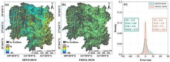
Figure 4.
Errors of the SRTM DEM (a) and the FREEL-corrected SRTM DEM (b) by comparing with the ICESat-2 and RTK reference elevations over Hunan Province; (c) histograms of the assessed errors of the original and the FREEL-corrected DEMs.
As is shown in Figure 4, the errors of the original SRTM DEM are varied from −81 m to 92 m, with an ME of 2.32 m, an MAE of 6.84 m, an STD of 9.43 m, and an RMSE of 9.75 m. Compared with the original SRTM DEM, the FREEL-corrected DEM has a narrow error range (between −68 m and 73 m). The ME of the FREEL-corrected DEM is about 0.01 m, which implies that the bias of the SRTM DEM products over Hunan Province can be effectively removed using the proposed FREEL framework. In addition, the variance matrices of the MAE, STD, and RMSE of the corrected SRTM DEM products are 3.78 m, 5.74 m, and 5.84 m, respectively, indicating an accuracy improvement of 45%, 39%, and 40% (with a mean of 41%). These results suggest that the FREEL framework is able to effectively mitigate the errors of the SRTM DEM products over Hunan Province.
Figure 5 plots four rose maps of the MEs of the original and the FREEL-corrected SRTM DEMs, with respect to four important features of vegetation coverage, canopy height, elevation, and slope, respectively. It can be seen from Figure 5 that the biases of the original SRTM DEM products (green lines) are varied from about 0.9 m to 15.2 m. In addition, the biases of the original SRTM DEM products over Hunan Province are highly related to these four features, that is, the biases are approximately increased with the increasing of elevations, the percentage of vegetation coverage, canopy heights, and slopes. With the use of the FREEL framework, the MEs of the corrected SRTM DEM range from 0.004 to 0.08, with a mean of 0.01. This result suggests that the proposed FREEL framework is able to well describe and further remove the biases of the SRTM DEM products in Hunan Province, even in those areas with dense vegetation coverage, high elevation and canopy, and mountainous terrain.
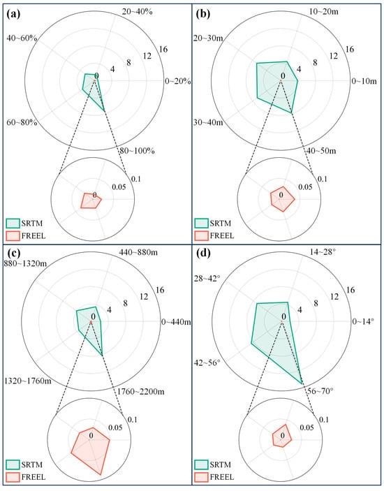
Figure 5.
Rose maps of the MEs of the original (green lines) and the FREEL-corrected SRTM DEM (red lines) with respect to the features of vegetation coverage (a), canopy height (b), elevation (c), and slope (d), respectively.
Figure 6 quantitatively demonstrates the efficacy of the FREEL framework in mitigating SRTM DEM errors through polar-coordinate STD analysis across vegetation density, canopy height, elevation, and slope parameters. The original DEM exhibits strong parameter-dependent error escalation, with the STDs increasing from 6.74 m to 12.38 m as the vegetation cover intensifies (0–20% to 80–100%) and surging from 8.98 m to 27.76 m with the slope steepness (0–14° to 56–70°). FREEL achieves a 39.1% reduction in mean STD (5.74 ± 0.83 m vs. 9.43 ± 2.15 m), maintaining sub-meter precision (5.12–5.97 m) even in extreme conditions (>80% vegetation; >56° slopes). Notably, it eliminates parameter-correlated error patterns (p > 0.05) and addresses critical limitations of SRTM through the following: (1) enhanced radar penetration compensation (canopy > 25 m), (2) improved topographic fidelity beyond design thresholds (slope > 45°), and (3) the resolution of nonlinear multivariate error interactions (R2 improvement > 0.72 vs. conventional methods). These advancements establish FREEL as a robust solution for DEM refinement in subtropical montane regions where coupled terrain–vegetation effects dominate error budgets [32,35], particularly benefiting ecological monitoring in sensitive zones.
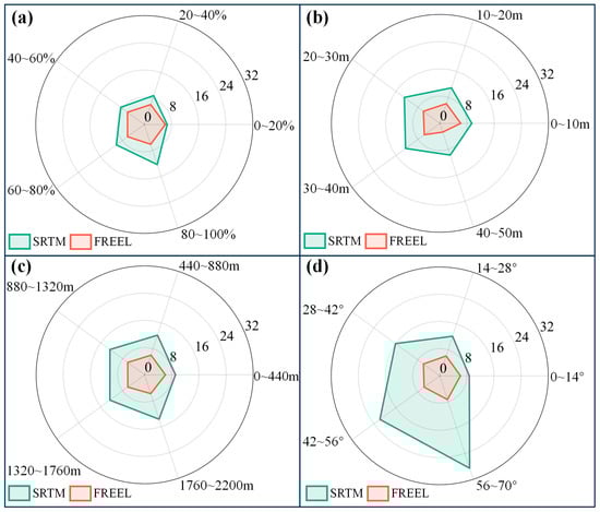
Figure 6.
Rose maps of the RMSEs of the original (green lines) and the FREEL-corrected SRTM DEM (red lines) with respect to the features of vegetation coverage (a), canopy height (b), elevation (c), and slope (d), respectively.
4. Discussion
4.1. Comparison with Mathematical Fitting Algorithms
As stated previously, it is a widely used strategy for correcting the errors of the SRTM DEM using mathematical fitting due to its simplicity and good interpretability. In this section, we compare the SRTM DEM products corrected by the FREEL framework and two classical mathematical fitting algorithms, i.e., linear regression (LR, see Equation (11)) [50] and nonlinear regression (NLR, see Equation (12)) [5].
where represents the elevation errors, denotes the regression coefficient, is the constant term, is the canopy height, is the LAI, is the slope, and is the vegetation coverage. Note that the same samples for the training and test of the FREEL framework in Section 3.3 are used for the DEM correction and accuracy validation based on the LR and NLR algorithms in this section for the sake of comparison.
Figure 7a,b plot the errors of the LR-corrected and NLR-corrected SRTM DEMs over Hunan Province by comparing with the SRTM DEM. Figure 7c shows the histogram of the errors of the LR-corrected and NLR-corrected SRTM DEMs. The calculated four error matrices of the LR- and NLR-corrected SRTM DEMs are listed in Table 1. As can be seen from Figure 7, the errors of the LR- and NLR-corrected SRTM DEMs are in the ranges from −74 m to 80 m and from −75 m to 77 m, which are both narrower than the error range of the original SRTM DEM products (i.e., between −81 m and 92 m). The LR-corrected DEM and NLR-corrected DEM exhibit substantial elevation deviations across the entire territory of Hunan Province, with particularly pronounced errors in the mountainous regions. However, a comparative assessment reveals that the NLR-corrected DEM achieves slightly better accuracy than the LR-corrected DEM in these high-relief areas, suggesting incremental improvements in its correction methodology for complex terrain features. It can be observed from Table 1 that the MEs of the LR- and NLR-corrected SRTM DEMs are all nearly equal to zero (i.e., 0.03 m and 0.02 m, respectively), indicating that the biases of the original SRTM DEM products can be effectively removed using the classical LR and NLR algorithms. Furthermore, the variance matrices (i.e., MAE, STD, and RMSE) of the LR- and NLR-corrected SRTM DEMs are all smaller than those of the original SRTM DEM products. This result further indicates that the LR and NLR algorithms are feasible for correcting the SRTM DEMs over Hunan Province.
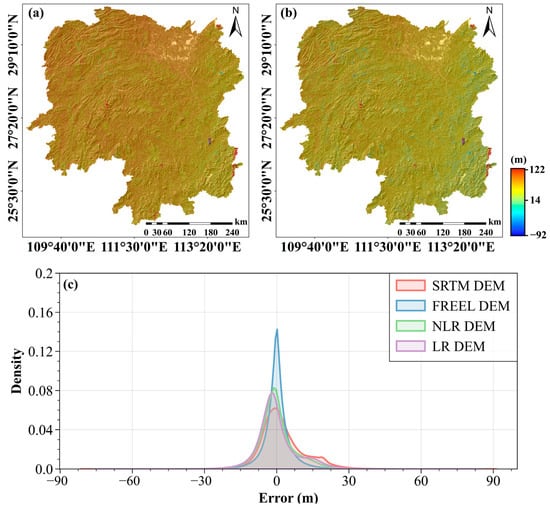
Figure 7.
The spatial error distribution of the NLR-corrected SRTM DEM (a) and LR-corrected SRTM DEM (b) compared with the SRTM DEM. The distribution of the vertical errors for the original SRTM DEM, FREEL-corrected, NLR-corrected, and LR-corrected SRTM DEMs (c).

Table 1.
The MEs, MAEs, RMSEs, and STDs of the SRTM DEM, FREEL-, LR- and NLR-corrected SRTM DEMs.
It is also noted from Table 1 that the MEs of the LR- and NLR-corrected SRTM DEMs are nearly equal to that of the FREEL-corrected SRTM DEM. Nevertheless, the variance matrices of the MAE, STD, and RMSE of the LR-corrected DEM are larger at 65%, 51%, and 53% (with a mean of 56%) than those matrices of the FREEL-corrected DEM. Moreover, the MAE, STD, and RMSE of the NLR-corrected DEM are larger at 49%, 39%, and 41% (with a mean of 43%) than the corresponding error matrices of the FREEL-corrected DEM. This result indicates that the proposed FREEL framework outperforms the LR and NLR fitting algorithms on SRTM DEM correction.
4.2. Comparison with Classical Machine Learning Algorithms
Machine learning algorithms are extensively used for SRTM DEM correction, especially in recent years, owing to their strong nonlinear fitting capability. In this section, three typical machine learning algorithms that have been used for DEM correction, i.e., the convolutional neural network (CNN) [51], backward propagation network (BPNN) [6], and feed-forward neural network (FNN) [8], have been chosen to be baselines to compare with the proposed FREEL framework. In addition, the DeepForest algorithm [33] that has not been utilized for DEM correction was selected to be a baseline algorithm in order to prove the advantage of the proposed AdDeepForest module.
In this section, the CNN algorithm is a standard U-Net, composed of an encoder with five convolutional layers and a decoder with five transposed convolutional layers, all of which use convolutional kernels of size 3. The BPNN algorithm contains five hidden layers, with 10, 20, 30, 50, and 10 hidden units, respectively, where the Levenberg–Marquardt algorithm was used for loss minimization during backpropagation. The FNN algorithm was composed of five hidden layers, where 15 neurons were designated in the hidden layers. The DeepForest algorithm consisted of 15 cascading layers, and each layer contained five random forests. Note that the same samples for the training and testing of the FREEL framework in Section 3.3 are used for the SRTM DEM correction and accuracy validation using the CNN, BPNN, FNN, and DeepForest algorithms in this section for the sake of comparison.
Figure 8 shows the errors of the DeepForest-, CNN-, BPNN-, and FNN-corrected SRTM DEMs over those testing points with ICESat-2 and/or RKT reference elevations. The histograms of these errors are shown in Figure 8e for comparison. The MEs, MAEs, RMSEs, and STDs of the corrected SRTM DEMs using different machine learning algorithms are listed in Table 2. For the sake of comparison, the corresponding error matrices of the original and the FREEL-corrected SRTM DEMs are added in Table 2. As is shown in Figure 8 and Table 2, the biases of the SRTM DEMs over Hunan Province can well be removed by these four machine learning algorithms due to the MEs of about zero (i.e., 0.02 m for the DeepForest, 0.01 m for the CNN, −0.02 m for the BPNN, and 0.03 m for the FNN). Meanwhile, the error range of the SRTM DEMs is narrowed between −75 m and 85 m, with respect to the original one from −81 m to 92 m. It can also be observed from Table 2 that the MAEs, RMSEs, and STDs of the CNN, BPNN, and FNN are approximately equal to each other, whereas all of these error matrices are larger than the corresponding ones of the DeepForest-corrected SRTM DEM. This result suggest that the DeepForest algorithm has a better performance on correcting the SRTM DEM products over Hunan Province, owing to its advantage of insensitivity on hyperparameter tuning and good robustness for small-scale training samples. The DeepForest-corrected DEM and CNN-corrected DEM demonstrate significantly higher accuracy across the entire Hunan Province compared to the BPNN-corrected DEM and FNN-corrected DEM. This performance contrast underscores the enhanced terrain modeling capabilities of deep learning-based correction approaches, particularly in regional-scale DEM applications involving complex geographical features.
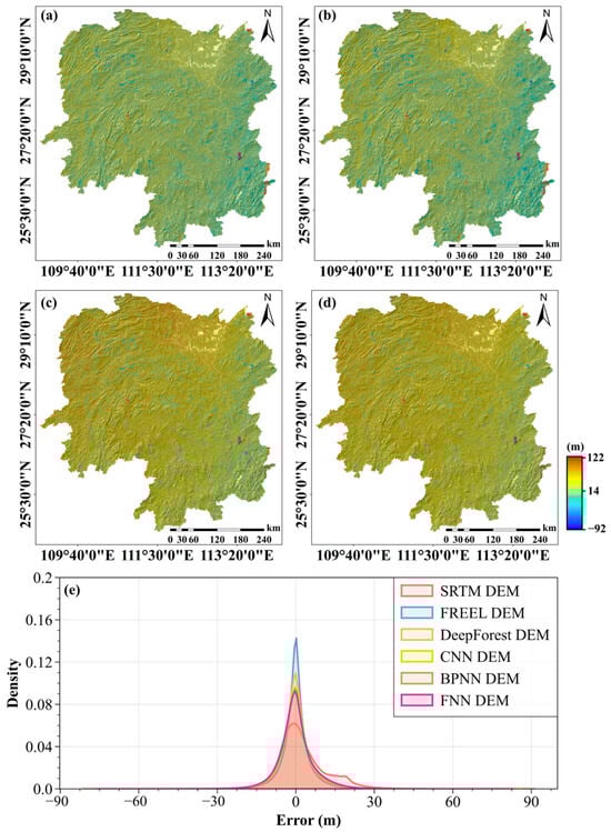
Figure 8.
The spatial error distribution of the DeepForest-corrected SRTM DEM (a), CNN-corrected SRTM DEM (b), BPNN-corrected SRTM DEM (c), and FNN-corrected SRTM DEM (d) compared with the SRTM DEM. The distribution of vertical errors for the original SRTM DEM, FREEL-corrected, DeepForest-corrected, CNN-corrected, BPNN-corrected, and FNN-corrected (e).
Table 2.
The MEs, MAEs, RMSEs, and STDs of the SRTM DEM, FREEL-, DeepForest-, CNN-, BPNN- and FNN-corrected SRTM DEMs.
Table 2 also shows that the MEs of the DeepForest-, CNN-, BPNN-, and FNN-corrected SRTM DEMs are approximately equal to the ME of the FREEL-corrected SRTM DEM. However, the variance matrices of the selected four machine learning algorithms are all larger than the corresponding error matrices of the FREEL-corrected SRTM DEM. More specifically, the MAE of the FREEL-corrected DEM is 3.78 m, indicating an improvement of 25% with respect to the mean MAE of the DEMs corrected by these four algorithms (i.e., 4.73 m). In addition, the RMSE and STD of the FREEL-corrected DEM (i.e., 5.82 m and 5.74 m, respectively) show an accuracy improvement of 21% and 23%, compared with the mean RMSE and STD of the DEMs corrected by these four algorithms (i.e., 7.06 m and 7.06 m, respectively). This result suggests that the proposed FREEL framework outperforms to correct the SRTM DEM products over Hunan Province, with respect to the DeepForest, CNN, BPNN, and FNN algorithms.
4.3. Comparison with Public Radar-Derived DEM Products
In recent years, several nearly global radar-derived DEM products generated by new InSAR data or improving from the original SRTM DEM have been released for the public. Typically, NASA reprocessed the InSAR data of the SRTM to generate new nearly global DEM products. Meanwhile, data gaps and some error sources (e.g., strip errors) have been corrected, with the aid of complementary products like ASTER GDEM and ICESat-2. In doing so, a new version of the SRTM DEM (referred to as “NASADEM”) was released in 2020 [52]. Except for the NASADEM products, some improved SRTM DEM products, where other typical errors (e.g., bias and spot noise) have been reduced, have been generated and openly published. Notable advancements in DEM error correction have been achieved through multisource data integration. Yamazaki et al. [53] systematically addressed absolute bias, stripe noise, spot noise, and elevation anomalies in open-access DEM products (including SRTM DEM V3, AW3D DEM, and Viewfinder Panoramas DEM) through the integration of multisource satellite observations and advanced filtering techniques. Their methodology yielded the Multi-Error-Removed Improved-Terrain (MERIT) DEM, featuring significantly improved vertical accuracy (±3.2 m RMSE) at a 30 m resolution. Building on this methodology, Hawker et al. [11] developed a building and vegetation removal framework for the TanDEM-X-derived Copernicus DEM (COPDEM30), implementing a machine learning framework employing random forest algorithms. This approach leveraged synergistic data from GEDI lidar and ICESat-2 photon-counting altimetry, culminating in the global Forest and Building-removed (FAB) DEM with enhanced bare-earth representation (89% artifact reduction).
In this section, we compare the FREEL-corrected SRTM DEM with the above-mentioned DEM products (i.e., NASADEM, MERIT DEM, and FAB DEM, see Figure 9b–d) over Hunan Province. For the fairness of the comparison, we corrected the original SRTM DEMs over Hunan Province using the FREEL framework based on the collected ICEsat-2 reference elevations only (70% for training and the remaining 30% for testing), instead of both ICESat-2 and RTK observations as done in Section 3.3. For the sake of clarity, the FREEL-corrected DEM based on ICESat-2 elevations only is referred to as the FREEL DEM (see Figure 9a). Figure 9e–h show the errors of the NASADEM, MERIT DEM, FAB DEM, and FREEL DEM by comparing with the same reference elevations for testing in Section 3.3. Figure 10 plots the histograms of the errors of these four DEM products, and the MEs, MAEs, RMSEs, and STDs of these four DEM products are listed in Table 3.
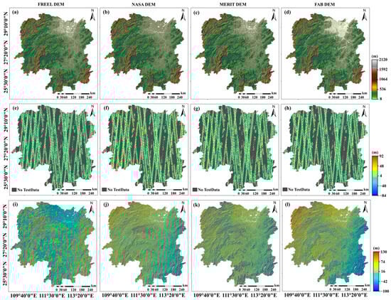
Figure 9.
The comparison of terrain variations for the FREEL-corrected SRTM DEM (a), NASA DEM (b), MERIT DEM (c), and FAB DEM (d). The spatial distribution of errors in relation to the reference elevation observations (ICESat-2 ATL08) in the test dataset for the FREEL-corrected SRTM DEM (e), NASA DEM (f), MERIT DEM (g), and FAB DEM (h), and the spatial error distribution of the FREEL-corrected SRTM DEM (i), NASA DEM (j), MERIT DEM (k), and FAB DEM (l) compared with the SRTM DEM.
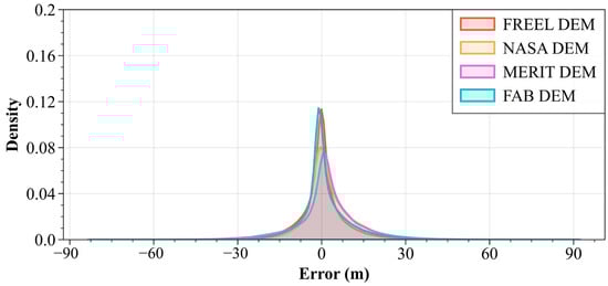
Figure 10.
Distribution of vertical error for original FREEL-corrected SRTM DEM, NASA DEM, MERIT DEM, and FAB DEM on the test dataset.
Table 3.
The MEs, MAEs, RMSEs, and STDs of the FREEL-corrected SRTM DEM, NASA DEM, MERIT DEM and FAB DEM.
As is shown in Figure 9 and Figure 10, and Table 3, the spatial distribution of the errors of these four DEM products is presented. More specifically, the MEs of the NASADEM, MERIT DEM, and FAB DEM are about 2.90 m, 1.99 m, and 1.20 m, implying that biases with different degrees are still contained in these three DEM products. It is noted that the ME of the NASADEM is nearly equal to the ME of the used SRTM DEM in Section 3.3 (i.e., 2.32 m), and it is larger than the MEs of the MERIT DEM and FAB DEM. This discrepancy primarily stems from differential elevation calibration methodologies. The NASA DEM retains inherent vertical biases due to the absence of systematic error correction, whereas both the MERIT DEM and FAB DEM incorporate rigorous elevation calibration protocols. Quantitative validation through four key error metrics (RMSE, MAE, ME, and STD) over Hunan Province demonstrates the FAB DEM’s superior performance, with RMSE reductions of 38–42% compared to the NASADEM and MERIT DEM (Table 3). This enhancement directly correlates with the FAB DEM’s assimilation of spaceborne photon-counting lidar data from ICESat-2 (error range: ±0.15 m) and full-waveform lidar observations from GEDI (vertical accuracy: ±1 m), which enabled pixel-level error correction through weighted least squares optimization. Moreover, the FREEL-corrected DEM demonstrates significant bias correction effectiveness in the mountainous regions of Hunan Province (Figure 9i), whereas noticeable elevation errors persist in the NASA-corrected DEM (Figure 9j), MERIT-corrected DEM (Figure 9k), and FAB-corrected DEM (Figure 9l) within these topographically complex areas. This comparative analysis highlights the superior terrain adaptation capability of the FREEL algorithm over existing correction methods when processing high-relief landscapes.
Figure 10 and Table 3 also show that the errors of the FREEL DEM are smaller than the remaining three open-accessed DEMs. For example, the ME of the FREEL DEM is about −0.07 m, indicating a mean improvement of about 98%, compared with the mean ME of the NASADEM, MERIT DEM, and FAB DEM over Hunan Province (i.e., 2.03 m). In addition, the MAE, RMSE, and STD of the FREEL DEM are 5.75 m, 9.27 m, and 9.27 m, showing improvements of around 17%, 14%, and 13%, respectively, with respect to the averaged MAE (6.94 m), RMSE (10.83 m), and STD (10.62 m) of the remaining three DEM products. It should be found from Table 3 that the ME of the corrected DEMs using the FREEL framework based on the ICESat-2 elevations is larger by about 85% than the ME of the FREEL-corrected DEM using both the ICESat-2 and RTK elevations. Furthermore, the remaining three error matrices of the former are also larger by about 36% than the latter. This result proves that more samples are helpful to improve the performance of machine learning training and prediction.
5. Conclusions
This paper introduces a novel machine learning framework termed FREEL, which was applied to the error correction of radar-derived DEM products to enhance the robustness of the correction process. The feasibility and performance of the FREEL framework were evaluated using SRTM DEM products over Hunan Province, leveraging extensive ICESat-2 and RTK reference elevation observations. The results indicate that the FREEL framework effectively mitigates bias in the SRTM DEM products for the region of interest and reduces error variance by approximately 41%. Comparisons with two classical mathematical fitting algorithms (i.e., LR and NLR) and four machine learning algorithms (i.e., CNN, BPNN, FNN, and DeepForest) for DEM correction suggest that while all these algorithms can effectively remove bias from the SRTM DEM over Hunan Province, the FREEL algorithm exhibits superior performance in reducing error variance, achieving improvements of 45% and 23% relative to the mathematical fitting and the machine learning algorithms, respectively. Finally, comparisons among three radar-derived DEM products over Hunan Province (i.e., NASADEM, MERIT DEM, and FAB DEM) reveal that the FREEL-corrected SRTM DEM exhibits 95% lower bias and 15% lower variance compared to these three products.
It is important to note that the FREEL framework integrates attention mechanisms, convolutional layers, and multiple DeepForest models to enhance feature extraction and improve the robustness of the error correction. However, this approach inevitably leads to increased algorithmic complexity and computational time consumption. In other words, while the FREEL framework achieves higher accuracy compared to classical machine learning algorithms, it does so at the expense of longer processing times. Therefore, optimizing the FREEL framework to reduce computational time will be a key focus of our future research. Additionally, the FREEL framework has been evaluated exclusively in Hunan Province, China, which covers an area larger than 285,000 . Although this region is substantial, testing the framework across a wider range of geographic areas would provide more comprehensive insights. We plan to conduct further tests in diverse regions in our future studies.
Author Contributions
Conceptualization, Z.O., C.Z. and Z.L.; methodology, Z.O., C.Z., D.Z. and Z.L.; validation, Z.O., C.Z., D.Z., Z.L., J.Z. and J.X.; formal analysis, Z.O., C.Z., Z.L. and J.Z.; investigation, Z.O., C.Z., Z.L. and J.Z.; data curation, D.Z. and J.Z.; writing—original draft preparation, Z.O.; writing—review and editing, Z.O., C.Z., D.Z. and Z.L.; supervision, C.Z. and D.Z.; project administration, C.Z., D.Z., Z.L. and J.Z.; funding acquisition, C.Z., Z.L. and J.Z. All authors have read and agreed to the published version of the manuscript.
Funding
This research was funded by the National Natural Science Foundation of China (Nos. 42474052, 42074016, and 42030112) and the Hunan Science Fund for Distinguished Young Scholars (2024JJ2100).
Data Availability Statement
The original contributions presented in the study are included in the article, further inquiries can be directed to the corresponding author.
Acknowledgments
We would like to thank the National Aeronautics and Space Administration (NASA) for providing the ICESat-2 ATL08 observations and the normalized difference vegetation index (NDVI) free of charge. We would also like to thank the United States Geological Survey (USGS) for the support of the SRTM DEM of Hunan Province. We are grateful to the leaf area index (LAI), land cover types, and canopy height datasets support from the “National Earth System Science Data Sharing Infrastructure, National Science & Technology Infrastructure of China (https://www.geodata.cn/main/, accessed on 25 March 2025)”, National Catalogue Service for Geographic information (https://www.webmap.cn/main.do?method=index, accessed on 25 March 2025), and Liu et al. (2022) [47], respectively. Moreover, many thanks to Minsi Ao from Hunan Province Mapping and the Science and Technology Investigation Institute for providing the CORS RTK Observations.
Conflicts of Interest
Di Zhang was employed by Tibet Huatailong Mining Development Co., Ltd. The remaining authors declare that the research was conducted in the absence of any commercial or financial relationships that could be construed as a potential conflict of interest.
References
- O’Loughlin, F.; Paiva, R.; Durand, M.; Alsdorf, D.; Bates, P. A multi-sensor approach towards a global vegetation corrected SRTM DEM product. Remote Sens. Environ. 2016, 182, 49–59. [Google Scholar] [CrossRef]
- Paul, F.; Huggel, C.; Kääb, A. Combining satellite multispectral image data and a digital elevation model for mapping debris-covered glaciers. Remote Sens. Environ. 2004, 89, 510–518. [Google Scholar] [CrossRef]
- Farr, T.G.; Rosen, P.A.; Caro, E.; Crippen, R.; Duren, R.; Hensley, S.; Kobrick, M.; Paller, M.; Rodriguez, E.; Roth, L.; et al. The shuttle radar topography mission. Rev. Geophys. 2007, 45, 183. [Google Scholar] [CrossRef]
- Berry, P.; Garlick, J.; Smith, R. Near-global validation of the SRTM DEM using satellite radar altimetry. Remote Sens. Environ. 2007, 106, 17–27. [Google Scholar] [CrossRef]
- Magruder, L.; Neuenschwander, A.; Klotz, B. Digital terrain model elevation corrections using space-based imagery and ICESat-2 laser altimetry. Remote Sens. Environ. 2021, 264, 112621. [Google Scholar] [CrossRef]
- Kulp, S.A.; Strauss, B.H. CoastalDEM: A global coastal digital elevation model improved from SRTM using a neural network. Remote Sens. Environ. 2018, 206, 231–239. [Google Scholar] [CrossRef]
- Pham, H.T.; Marshall, L.; Johnson, F.; Sharma, A. A method for combining SRTM DEM and ASTER GDEM2 to improve topography estimation in regions without reference data. Remote Sens. Environ. 2018, 210, 229–241. [Google Scholar] [CrossRef]
- Wendi, D.; Liong, S.; Sun, Y.; Doan, C.D. An innovative approach to improve SRTM DEM using multispectral imagery and artificial neural network. J. Adv. Model. Earth Syst. 2016, 8, 691–702. [Google Scholar] [CrossRef]
- Li, Y.; Li, L.; Chen, C.; Liu, Y. Correction of global digital elevation models in forested areas using an artificial neural network-based method with the consideration of spatial autocorrelation. Int. J. Digit. Earth 2023, 16, 1568–1588. [Google Scholar] [CrossRef]
- Warner, D.L.; Callahan, J.A.; McKenna, T.E.; Medlock, C. Reducing vertical bias and error in tidal marsh digital elevation models with machine learning and LiDAR derivatives. Estuar. Coast. Shelf Sci. 2023, 291, 108442. [Google Scholar] [CrossRef]
- Hawker, L.; Uhe, P.; Paulo, L.; Sosa, J.; Savage, J.; Sampson, C.; Neal, J. A 30 m global map of elevation with forests and buildings removed. Environ. Res. Lett. 2022, 17, 024016. [Google Scholar] [CrossRef]
- Rogers, J.N.; Parrish, C.E.; Ward, L.G.; Burdick, D.M. Improving salt marsh digital elevation model accuracy with full-waveform lidar and nonparametric predictive modeling. Estuar. Coast. Shelf Sci. 2018, 202, 193–211. [Google Scholar] [CrossRef]
- Dong, W.; Wang, P.; Yin, W.; Shi, G.; Wu, F.; Lu, X. Denoising prior driven deep neural network for image restoration. IEEE Trans. Pattern Anal. Mach. Intell. 2018, 41, 2305–2318. [Google Scholar] [CrossRef] [PubMed]
- Zhang, Q.; Yang, L.T.; Chen, Z.; Li, P. A survey on deep learning for big data. Inf. Fusion 2018, 42, 146–157. [Google Scholar] [CrossRef]
- Ao, M.; Dong, M.; Chu, B.; Zeng, X.; Li, C. Revealing the user behavior pattern using HNCORS RTK location big data. IEEE Access 2019, 7, 30302–30312. [Google Scholar] [CrossRef]
- Narasimhan, R.; Stow, D. Daily MODIS products for analyzing early season vegetation dynamics across the North Slope of Alaska. Remote Sens. Environ. 2010, 114, 1251–1262. [Google Scholar] [CrossRef]
- Zou, L.; Tian, F.; Liang, T.; Eklundh, L.; Tong, X.; Tagesson, T.; Dou, Y.; He, T.; Liang, S.; Fensholt, R. Assessing the upper elevational limits of vegetation growth in global high-mountains. Remote Sens. Environ. 2023, 286, 113423. [Google Scholar] [CrossRef]
- Joshi, P.; Mukherjee, S.; Ghosh, A.; Garg, R.; Mukhopadhyay, A. Evaluation of vertical accuracy of open source Digital Elevation Model (DEM). Int. J. Appl. Earth Obs. Geoinf. 2013, 21, 205–217. [Google Scholar] [CrossRef]
- Gdulová, K.; Marešová, J.; Moudrý, V. Accuracy assessment of the global TanDEM-X digital elevation model in a mountain environment. Remote Sens. Environ. 2020, 241, 111724. [Google Scholar] [CrossRef]
- Toutin, T. Impact of terrain slope and aspect on radargrammetric DEM accuracy. ISPRS J. Photogramm. Remote Sens. 2002, 57, 228–240. [Google Scholar] [CrossRef]
- Li, Y.; Zeng, H.; Zhang, M.; Wu, B.; Zhao, Y.; Yao, X.; Cheng, T.; Qin, X.; Wu, F. A county-level soybean yield prediction framework coupled with XGBoost and multidimensional feature engineering. Int. J. Appl. Earth Obs. Geoinf. 2023, 118, 103269. [Google Scholar] [CrossRef]
- Liu, D.; Hua, G.; Viola, P.; Chen, T. Integrated feature selection and higher-order spatial feature extraction for object categorization. In Proceedings of the 2008 IEEE Conference on Computer Vision and Pattern Recognition, Anchorage, AK, USA, 23–28 June 2008; pp. 1–8. [Google Scholar]
- Memisevic, R. Gradient-based learning of higher-order image features. In Proceedings of the 2011 International Conference on Computer Vision, Barcelona, Spain, 6–13 November 2011; pp. 1591–1598. [Google Scholar]
- Zeng, H.; Cheung, Y.-M. Feature selection and kernel learning for local learning-based clustering. IEEE Trans. Pattern Anal. Mach. Intell. 2010, 33, 1532–1547. [Google Scholar] [CrossRef] [PubMed]
- Tian, L.; Xue, B.; Wang, Z.; Li, D.; Yao, X.; Cao, Q.; Zhu, Y.; Cao, W.; Cheng, T. Spectroscopic detection of rice leaf blast infection from asymptomatic to mild stages with integrated machine learning and feature selection. Remote Sens. Environ. 2021, 257, 112350. [Google Scholar] [CrossRef]
- Shao, Z.; Yang, S.; Gao, F.; Zhou, K.; Lin, P. A new electricity price prediction strategy using mutual information-based SVM-RFE classification. Renew. Sustain. Energy Rev. 2017, 70, 330–341. [Google Scholar] [CrossRef]
- Hansen, M.C.; Loveland, T.R. A review of large area monitoring of land cover change using Landsat data. Remote Sens. Environ. 2012, 122, 66–74. [Google Scholar] [CrossRef]
- Yuan, Q.; Shen, H.; Li, T.; Li, Z.; Li, S.; Jiang, Y.; Xu, H.; Tan, W.; Yang, Q.; Wang, J.; et al. Deep learning in environmental remote sensing: Achievements and challenges. Remote Sens. Environ. 2020, 241, 111716. [Google Scholar] [CrossRef]
- Zhong, L.; Hu, L.; Zhou, H. Deep learning based multi-temporal crop classification. Remote Sens. Environ. 2019, 221, 430–443. [Google Scholar] [CrossRef]
- Vaswani, A.; Shazeer, N.; Parmar, N.; Uszkoreit, J.; Jones, L.; Gomez, A.N.; Kaiser, Ł.; Polosukhin, I. Attention is all you need. In Proceedings of the Advances in Neural Information Processing Systems, Long Beach, CA, USA, 4–9 December 2017; Volume 30. [Google Scholar]
- Xu, J.; Zhu, Y.; Zhong, R.; Lin, Z.; Xu, J.; Jiang, H.; Huang, J.; Li, H.; Lin, T. DeepCropMapping: A multi-temporal deep learning approach with improved spatial generalizability for dynamic corn and soybean mapping. Remote Sens. Environ. 2020, 247, 111946. [Google Scholar] [CrossRef]
- Zhou, G.; Chen, W.; Gui, Q.; Li, X.; Wang, L. Split depth-wise separable graph-convolution network for road extraction in complex environments from high-resolution remote-sensing images. IEEE Trans. Geosci. Remote Sens. 2021, 60, 1–15. [Google Scholar] [CrossRef]
- Zhou, Z.-H.; Feng, J. Deep forest. Natl. Sci. Rev. 2019, 6, 74–86. [Google Scholar] [CrossRef]
- Utkin, L.V.; Kovalev, M.S.; Meldo, A.A. A deep forest classifier with weights of class probability distribution subsets. Knowledge-Based Syst. 2019, 173, 15–27. [Google Scholar] [CrossRef]
- Xiao, C.; Chen, N.; Hu, C.; Wang, K.; Gong, J.; Chen, Z. Short and mid-term sea surface temperature prediction using time-series satellite data and LSTM-AdaBoost combination approach. Remote Sens. Environ. 2019, 233, 111358. [Google Scholar] [CrossRef]
- Rabus, B.; Eineder, M.; Roth, A.; Bamler, R. The shuttle radar topography mission—A new class of digital elevation models acquired by spaceborne radar. ISPRS J. Photogramm. Remote Sens. 2003, 57, 241–262. [Google Scholar] [CrossRef]
- Neuenschwander, A.; Guenther, E.; White, J.C.; Duncanson, L.; Montesano, P. Validation of ICESat-2 terrain and canopy heights in boreal forests. Remote Sens. Environ. 2020, 251, 112110. [Google Scholar] [CrossRef]
- Tian, X.; Shan, J. Comprehensive evaluation of the ICESat-2 ATL08 terrain product. IEEE Trans. Geosci. Remote Sens. 2021, 59, 8195–8209. [Google Scholar] [CrossRef]
- Yu, J.; Nie, S.; Liu, W.; Zhu, X.; Lu, D.; Wu, W.; Sun, Y. Accuracy assessment of ICESat-2 ground elevation and canopy height estimates in mangroves. IEEE Geosci. Remote Sens. Lett. 2021, 19, 1–5. [Google Scholar] [CrossRef]
- Ao, M.; Zeng, X.; Chen, C.; Chu, B.; Zhang, Y.; Zhou, C. Identification of The Survey Points from Network RTK Trajectory with Improved DBSCAN Clustering, Case Study on HNCORS. Earth Sci. Inform. 2023, 16, 1835–1847. [Google Scholar] [CrossRef]
- Snay, R.A.; Soler, T. Continuously operating reference station (CORS): History, applications, and future enhancements. J. Surv. Eng. 2008, 134, 95–104. [Google Scholar] [CrossRef]
- Teunissen, P.J.; Odijk, D.; Zhang, B. PPP-RTK: Results of CORS network-based PPP with integer ambiguity resolution. J Aeronaut Astronaut. Aviat. Ser. 2010, 42, 223–230. [Google Scholar]
- Su, Y.; Guo, Q.; Ma, Q.; Li, W. SRTM DEM correction in vegetated mountain areas through the integration of spaceborne LiDAR, airborne LiDAR, and optical imagery. Remote Sens. 2015, 7, 11202–11225. [Google Scholar] [CrossRef]
- Song, W.; Mu, X.; Ruan, G.; Gao, Z.; Li, L.; Yan, G. Estimating fractional vegetation cover and the vegetation index of bare soil and highly dense vegetation with a physically based method. Int. J. Appl. Earth Obs. Geoinf. 2017, 58, 168–176. [Google Scholar] [CrossRef]
- Chen, J.; Chen, J.; Liao, A.; Cao, X.; Chen, L.; Chen, X.; He, C.; Han, G.; Peng, S.; Lu, M.; et al. Global land cover mapping at 30 m resolution: A POK-based operational approach. ISPRS J. Photogramm. Remote Sens. 2015, 103, 7–27. [Google Scholar] [CrossRef]
- Shafizadeh-Moghadam, H.; Minaei, M.; Feng, Y.; Pontius, R.G., Jr. GlobeLand30 maps show four times larger gross than net land change from 2000 to 2010 in Asia. Int. J. Appl. Earth Obs. Geoinf. 2019, 78, 240–248. [Google Scholar] [CrossRef]
- Liu, X.; Su, Y.; Hu, T.; Yang, Q.; Liu, B.; Deng, Y.; Tang, H.; Tang, Z.; Fang, J.; Guo, Q. Neural network guided interpolation for mapping canopy height of China’s forests by integrating GEDI and ICESat-2 data. Remote Sens. Environ. 2022, 269, 112844. [Google Scholar] [CrossRef]
- Xiao, Z.; Liang, S.; Wang, J.; Chen, P.; Yin, X.; Zhang, L.; Song, J. Use of general regression neural networks for generating the GLASS leaf area index product from time-series MODIS surface reflectance. IEEE Trans. Geosci. Remote Sens. 2013, 52, 209–223. [Google Scholar] [CrossRef]
- Su, Y.; Guo, Q. A practical method for SRTM DEM correction over vegetated mountain areas. ISPRS J. Photogramm. Remote Sens. 2014, 87, 216–228. [Google Scholar] [CrossRef]
- Nguyen, N.S.; Kim, D.E.; Jia, Y.; Raghavan, S.V.; Liong, S.Y. Application of Multi-Channel Convolutional Neural Network to Improve DEM Data in Urban Cities. Technologies 2022, 10, 61. [Google Scholar] [CrossRef]
- Buckley, S.; Agram, P.; Belz, J.; Crippen, R.; Gurrola, E.; Hensley, S.; Kobrick, M.; Lavalle, M.; Martin, J.; Neumann, M. DOCUMENT CHANGE LOG; LP DAAC: Sioux Falls, SD, USA, 2022. [Google Scholar]
- Crippen, R.; Buckley, S.; Agram, P.; Belz, E.; Gurrola, E.; Hensley, S.; Kobrick, M.; Lavalle, M.; Martin, J.; Neumann, M.; et al. NASADEM global elevation model: Methods and progress. Int. Arch. Photogramm. Remote Sens. Spat. Inf. Sci. 2016, 41, 125–128. [Google Scholar] [CrossRef]
- Yamazaki, D.; Ikeshima, D.; Sosa, J.; Bates, P.D.; Allen, G.H.; Pavelsky, T.M. MERIT Hydro: A high-resolution global hydrography map based on latest topography dataset. Water Resour. Res. 2019, 55, 5053–5073. [Google Scholar] [CrossRef]
Disclaimer/Publisher’s Note: The statements, opinions and data contained in all publications are solely those of the individual author(s) and contributor(s) and not of MDPI and/or the editor(s). MDPI and/or the editor(s) disclaim responsibility for any injury to people or property resulting from any ideas, methods, instructions or products referred to in the content. |
© 2025 by the authors. Licensee MDPI, Basel, Switzerland. This article is an open access article distributed under the terms and conditions of the Creative Commons Attribution (CC BY) license (https://creativecommons.org/licenses/by/4.0/).