Classical vs. Machine Learning-Based Inpainting for Enhanced Classification of Remote Sensing Image

Abstract

Inpainting is a technique that allows for the reconstruction of images and the removal of unnecessary elements. In our research, we employed inpainting to eliminate erroneous lines in the images and examined its abilities in improving classification quality. To reduce the erroneous lines, we designed ResGMCNN, whose multi-column generator model uses residual blocks. For our studies, we used data from the COWC and DOTA datasets. The GMCNN model with residual connections outperformed most classical inpainting methods, including the Telea and Navier–Stokes methods, achieving a maximum structural similarity index measure (SSIM) of 0.93. However, despite the improvement in filling quality, these results still lag behind the Criminisi method, which achieved the highest SSIM values (up to 0.99). We investigated the improvement in classification quality by removing vehicles from the road class in images acquired by UAVs. For vehicle removal, we used Criminisi inpainting, as well as Navier–Stokes and Telea for comparison. Classification was performed using eight classifiers, six of which were based on machine learning, where we proposed our solutions. The results showed that classification quality could be improved by several to over a dozen percent, depending on the metric, image, and classification method. The F1-score and Cohen Kappa metrics indicated an improvement in classification quality of up to 13% in comparison to the classification of the original image. Nevertheless, each of the classical inpainting methods examined improved the road classification.

1. Introduction

In recent years, technological advancements have significantly improved the acquisition and processing of diverse imaging data. Satellite and low-altitude imaging are utilised for research on climate change, land and ocean observation, crisis management, and public safety. This is made possible by rapidly evolving computing technology and algorithms. By integrating imaging data with various processing methods and algorithms based on deep convolutional networks, it is possible to automatically detect and classify objects, segment objects, and quantitative and qualitative analysis of images. Recently, much research has focused on the use of deep networks (for example, GANs) for change detection [1,2,3]. Another application of artificial intelligence algorithms is the reconstruction of lost image fragments, for example, due to cloud cover, shadowing of other objects, or the intentional concealment of a specific area or object. In this article, we propose the use of inpainting to enhance classification quality. Inpainting allows for the concealment of an object in an image by replacing the object’s pixels with new pixels whose values depend on the surrounding pixels (background). Naturally, there are many inpainting techniques, and the choice of method significantly influences the outcome. In this research, it is crucial to select an inpainting method such that the removed pixels are replaced with pixels that closely match the properties of the surrounding pixels. The better the matching of pixel properties, the higher the likelihood of improving classification quality.

We consider the discussed issue in two ways: First, we focus on the reconstruction of images with erroneous lines and propose a new method for removing linear objects from images. We study the effectiveness of six methods (three classical and three GAN-based methods) based on visual analysis and SSIM. This provides an opportunity to select effective methods that do not cause blurring in the image. Based on this, we further propose an effective inpainting method for removing area objects that disrupt classification in images, which we investigate through the example of removing cars and improving road classification. In our research, we consider the example of removing cars from the roadway, which we explore using the example of removing cars and improving road classification. A well-executed inpainting will make it possible to remove vehicles and paint them so that the roadway is continuous, not intersected by objects (cars) or parts of them. Then, after classification, the road class, too, will be more consistent and free from noise caused by the occurrence of objects of other classes.

In the first part of the investigation, we removed erroneous lines from the image. These are often registration errors where a detector flaw has prevented the complete capture of the image. The lines then appear as stripes with pixel values equal to 0. Similar errors may also be intentional, aimed at concealing selected information within the image. Such lines disrupt the image and its subsequent processing. Inpainting can be one of the methods to fill these gaps. In this article, we present a new method to correct erroneous lines in images. To successfully fill in the missing fragments of the image, generative adversarial networks (GANs) can be effectively utilised [4]. One solution is the Generative Multi-column Convolutional Neural Network (GMCNN), proposed by Wang Yi’s team in 2018 [5]. It has a multi-column structure [6,7], which allows the division of the image into components with different receptive fields and feature resolutions. However, this solution does not enable the reconstruction of missing parts of images in such a way that the new pixel values are indistinguishable from the rest of the image. Furthermore, attempts to adjust other parameters used during the training of the network have not yielded the expected results. To enhance the performance of GMCNN, we propose a modification of the generator model, which allows for significantly more accurate filling of the missing fragments of the image, making their identification impossible.

In the second part of the research, we focus on selecting an inpainting method that enables a precise reconstruction of the image after the removal of surface objects that degrade classification quality. This problem is clearly visible in images of roads captured from low altitudes in areas with high traffic density. The vehicles measure from dozens to hundreds of pixels, making them relatively large objects. Additionally, they are imaged by pixels with very diverse spectral properties, significantly different from the properties of the pixels depicting the road. This results in the classified road object being inconsistent, interrupted by objects from other classes (which are actually vehicles on the road). This is detrimental to future work on the classified image, such as automatic surface and shape analysis of roads or automatic vectorisation of road networks. Therefore, in this article, we propose the application of inpainting in remote sensing to remove unnecessary objects (vehicles) from the background (road). Until now, inpainting has mainly been used for artistic purposes and in computer vision (to conceal objects in an image) [8] or for military and security purposes (masking protected objects whose concealment is important for security reasons). Correct classification is an important and current issue. Currently, there is a trend in science and technology towards the automation of many processes, which is justified by the savings in time and costs.

Section 2 of this article contains a review of the current research and methods related to inpainting in remote sensing. Section 3 describes the data used in the studies. Section 4 presents the experiment: a detailed description of the methodology used and the results. This section is divided into subsections, which sequentially show the research and results for the reduction in erroneous lines in the image and for the application of inpainting to improve classification quality using road examples. This section includes a comparison of different inpainting techniques and classification results before and after image reconstruction using various classifiers. Section 5 and Section 6 contain the discussion and conclusions, respectively.

2. Related Works

Over the years, many methods for concealing objects in images have developed. Their foundation consists of simple copy–move techniques, where the unwanted object is removed and another fragment of the image is pasted in its place. This solution is very popular due to its simplicity, but unfortunately, it has many limitations and is unsuitable for the precise processing of complex images [8]. The first, simplest methods for removing and filling objects from the background can be divided into two groups: texture synthesis algorithms for generating large areas of the image from texture samples, and painting techniques for filling small gaps in the image. Texture synthesis methods were designed for repetitive two-dimensional patterns with some stochasticity. Painting methods treat linear structures (lines and contours) as one-dimensional patterns [9].

In the contemporary literature, inpainting methods are divided into sequential-based methods and methods based on Convolutional Neural Networks (CNNs) or generative adversarial networks (GANs) [8,10]. Sequential-based methods are traditional methods based on a combination of various image processing techniques. This group primarily includes exemplar-based synthesis methods, which are an extension and combination of texture synthesis and painting algorithms. The first solutions of this type depended on the order of the filling of the pixels based on the texturing level of the surrounding pixels or the local shape of the target area [11,12]. Subsequently, methods based on texture segmentation and algorithms for the parallel synthesis of composite textures were developed [9,13,14].

Sequential-based methods can be divided into two categories: patch-based and diffusion-based methods [8]. Patch-based methods fill in the image patch by patch, with missing areas being completed by the most suitable candidate patches copied from the original part of the image. This category includes various solutions focusing on different ways of selecting the most appropriate candidate patch, which are based, among other factors, on texture analysis [15,16,17,18] regularisation [19] and the assessment of significance and probability [20,21]. The MAP algorithm [22] creates a likelihood probability density function (PDF) based on a linear observation model, while a robust Huber–Markov model is used as the prior PDF. A more advanced solution that yields satisfactory results in reconstructing areas that are not visible due to cloud cover or shading is the Bandelet-Based Inpainting Technique [23]. This two-step technique, based on Bandelet transformation and multi-scale geometric clustering, allows for the restoration of parts of the Earth’s surface obscured by clouds. However, the reconstructed areas can be easily identified in the images. Additionally, various patch-based methods have been proposed that simultaneously aim to reduce distortions in the image, such as noise, textures, and scratches [24,25]. Unfortunately, distortion-reducing methods often lead to image blurring, which has prompted the proposal of alternative solutions for filling in removed areas based on the simultaneous analysis of structure and texture [9,26], which do not introduce additional blurring. In particular, the approach proposed by Criminisi et al. [9] deserves attention. It is a relatively straightforward solution that provides good results without blurring the image. The actual colour values are computed using pattern synthesis, and the simultaneous propagation of texture and structure information is achieved through a single, efficient algorithm. The approach is based on a pattern-based texture synthesis that depends on a unified scheme for determining the order of filling. The method, according to its authors, is effective for both linear structures and 2-dimensional textures. A significant disadvantage of the Criminisi method is its high computational complexity and therefore long image reconstruction time. The Criminisi method is time-consuming, especially if a lot of non-adjacent elements are removed from the image. Structure and texture propagation must be performed for each element. The method uses the “best-first” algorithm, so for each painted element, it is necessary to perform an analysis to find the best match. In addition, in the Criminisi method, filling runs iteratively until all the empty pixels are filled, which also makes it a lengthy computational process. Occasionally, it may not be possible to find a replacement patch similar to the missing area. For this reason, image painting has been proposed, which involves finding an image with similar semantics from an existing image library and then selecting the appropriate correction information to transfer to the target image [10,27].

Diffusion-based methods fill in the empty area by smoothly propagating the content of the image from the boundary to the interior of the missing region. The reconstruction of missing parts of the image is usually limited by the information surrounding the hole. These methods are effective for simple images and small holes, but when the image contains a lot of texture and objects, they may not yield satisfactory results. The most popular solutions are based on the analysis of local statistics, Fourier transformation, or Navier–Stokes equations [8,10,28,29,30,31]. These methods are usually faster than the Criminisi method, but less effective. The Navier–Stokes method [31] employs classical fluid dynamics to dynamically propagate isophotes from the edge to the centre of the region to be filled. The guiding principle is to treat the image intensity as a “stream function” for two-dimensional incompressible flow. The Laplacian of the image intensity plays the role of fluid vorticity—it is transferred into the region to be filled by a vector field defined by the stream function. The Navier–Stokes algorithm is designed to continue the isophotes while simultaneously matching the gradient vectors at the boundary of the painting region. In the Navier–Stockes method, the prediction of the correct texture is based on the theory of fluid flow, which may not always correspond to the actual textural characteristics, especially in the case of large and irregular holes, where the fill is not a uniform texture. Meanwhile, the method by Alexandru Telea [30] allows for filling small areas of the image and produces results very similar to the aforementioned Navier–Stokes method, but it is significantly faster and simpler to implement. It is based on the propagation of an image smoothness estimator along the image gradient (similar to the Bertalmio method [32]). This algorithm defines the image smoothness as a weighted average of the pixels surrounding the area to be filled. Missing regions are treated as contour lines for which the fast marching method (FMM) is used to fill in the image information. Filling is a function of the boundary values surrounding the hole, so for large holes or areas of complicated texture, the method can have difficulty with faithful reconstruction. Instead of accurately reproducing texture details, the method often creates a simplified version of the texture. Some details may be lost, and the edges of objects on the edges of holes may be blurred.

Inpainting methods based on Convolutional Neural Networks (CNNs) and generative adversarial networks (GANs) are relatively new solutions that have emerged alongside the development of neural networks and machine learning techniques. These methods rely on learning information about the high and low-frequency features of the damaged image, as well as the structural and textural coherence of the image. By incorporating various conditions, it is possible to generate new features that complement the damaged area [8,10]. Early solutions focused on inpainting regular rectangular holes and narrow gaps [33]. Later, approaches were developed to fill in irregular areas [34,35,36]. The operation of algorithms based on deep neural networks differs somewhat from the classical approaches. Classical algorithms work with two types of data: input and output. Computers take input data for calculations and then provide the results of their actions in the form of output data. In the case of machine learning (or neural networks, which are a subcategory of machine learning), the algorithm takes both input and output data and, as a result, creates a new (usually improved) version of itself. Among the algorithms that enable the filling of missing image fragments using generative adversarial networks (GANs), there is significant diversity. One solution is the iterative filling of missing regions by searching for the best sample from the remaining part of the image, where a fixed patch size is used primarily [9,37]. Another method involves selecting the best filling by applying global matching for only one patch during iterations, resulting in a low efficiency for this method. A solution to these problems is the method based on Multi-Patch Match with Adaptive Size [38], which first assesses the inhomogeneity of the image and adjusts the patch size accordingly. Another proposed solution to this problem is the Sdf-MAN architecture [39], which combines disparity maps from different sources while simultaneously implementing complementary information. The discriminator model of this algorithm utilises various dimensions of receptive fields and other scales, and the use of a random Markov field for the enhanced disparity map provides better estimates of the true disparity distribution. Another improvement to the generated results is the use of a two-stage loss function that prevents colour discrepancies from appearing in the image [40]. This function consists of various Gaussian kernels that are used at different stages of the network, allowing for the restoration of image details. Another solution is the use of a generator model composed of multiple columns, enabling a more detailed filling of image fragments [41]. However, most of the presented solutions do not address the problem of reconstructing fragments of satellite imagery. Nevertheless, A. Kuznetsov and M. Gashnikov [42] note in their article that generative neural networks successfully handle the reconstruction of fragments of imagery, leading to the creation of forgery in Earth remote sensing data. Machine learning-based methods are effective; however, a significant limitation is the requirement for large datasets to train the networks. Training a network necessitates the careful preparation of training and testing data and considering various conditions, and it is a very time-consuming process.

With the advancement in image processing techniques, research is emerging regarding the application of inpainting in various remote sensing tasks. Due to the wide development of machine learning, these publications focus specifically on these techniques. In the context of satellite analyses, inpainting can encompass filling in missing data, reconstructing textures and structures, and improving the quality of image analysis [43]. Filling in missing data often occurs due to atmospheric obstacles, such as clouds [44,45]. At such times, parts of the Earth’s surface may be undetectable in satellite images. Inpainting methods based on machine learning are often used to reconstruct images in cloud-covered areas. In recent years, research has emerged on the use of deep learning for this task, mainly CNNs and GANs. Zhang et al. [46] proposed synthesising Sentinel-1 SAR data with a CNN model. In turn, Ma et al. [47] designed an aliency enhancement model to replace the original CNN module in CycleGAN. This improved the calibration of attention channel weights and captured detailed information for multi-level feature maps. More recent studies have proposed applied deep learning techniques, in particular, superpixel segmentation and generative adversarial networks (GANs) [48], multi-stream complementary generative adversarial network (MSC-GAN) for cloud removal using multi-temporal data [49], Hybrid Attention Generative Adversarial Network (HyA-GAN) [50]. HyA-GAN combines the channel attention mechanism and spatial attention mechanism to form a generative adversarial network [50]. Due to the different shapes, structures and spectral properties of clouds and cars, approaches dedicated to inpainting in the cloud area may not be effective for removing cars from the image. Due to the different spectral properties of objects, it is necessary to generate their masks in a different way. In addition, differences in size and shape (clouds are larger and more irregular) may cause different effectiveness of inpainting methods. Moreover, the structure of the reconstructed areas is quite different. Roadways have a rather homogeneous structure, while under the clouds, there is generally a very different fragment of the image hidden. Therefore, for cloud removal, machine learning-based methods are more effective than classical inpainting methods, which may not be true for removing cars from the road.

Inpainting allows for the filling of these missing fragments, improving the coherence and continuity of the data. In cases of data corruption or artefacts in satellite images, the inpainting technique can assist in reconstructing natural patterns, such as forested areas, water bodies, or urban structures. Moreover, the application of inpainting can enhance image quality and increase its usability for further analyses.

3. Data

In this research, various types of data were utilised. In the first part of the study (reduction in erroneous lines), aerial and satellite image datasets were employed. To test the method on different types of data, two additional databases were used. The first was DOTA-v1.5 (Dataset for Object Detection in Aerial Images) [51], which includes aerial images captured by various platforms, including UAV (Unnamed Aerial Vehicle) systems. Although it was originally developed for object detection, its features, such as high resolution and diversity of objects, also make it applicable for segmentation tasks. The second database was COWC (Cars Overhead With Context), which consists of aerial images obtained from various platforms, including UAV systems [52]. This dataset is intended for the analysis of aerial photographs and satellite imagery, containing detailed information about vehicles visible in the images. The third dataset, used solely for verifying inpainting methods, was an original image database created based on a satellite scene captured by WorldView-2. It included segments depicting diverse areas such as fields, meadows, and forests, allowing for the evaluation of the algorithm’s performance in the context of different types of terrain. Both datasets were used to prepare and test the ResGMCNN (Residual Generative Multi-column Convolutional Neural Network) model. As a part of this process, the images were divided into smaller fragments of 256 × 256 pixels, which was dictated by the input requirements of the network. Additionally, to simulate the presence of artefacts and areas requiring masking, a set of masks from the NVIDIA Irregular Mask Dataset [34] was applied. This allowed for the introduction of irregular structures into the images, enhancing the realism of the simulated gaps and enabling a better assessment of the inpainting method’s effectiveness.

In the subsequent part of the investigation (removal of unnecessary objects from the background), data obtained by UAVs at various altitudes were used. Flights were carried out in an urban area along a national road with high traffic density and in a densely built area intersected by streets, where a significant number of cars can also be observed on the road, especially during peak hours.

The images were acquired during two photogrammetric flights. Flight 1 was carried out on the S12 expressway in Poland (the city of Radom). Expressways are designed for vehicular traffic and typically exhibit a high volume of traffic, particularly in urban areas. Radom is located in central-eastern Poland, with a population density of approximately 1774.5 inhabitants/km² [53]. Flight 2 was carried out on residential streets in Warsaw. Warsaw is the capital of Poland and the largest city in the country, with a population density of around 3602 inhabitants/km² [53]. Due to the high population density, the streets in the city are often congested during peak hours, resulting in a noticeable increase in traffic volume. The location of these cities in the central part of the country (Figure 1) is an additional factor that contributes to increased street traffic. Central Poland serves as a good transit point between the eastern and western parts of the country, as well as between the southern and northern regions. There are many logistics halls and reloading places in central Poland, which is also very important in terms of monitoring street traffic.

Both datasets were acquired from the UAV platform. Flight 1 was executed using the WingtraOne platform equipped with a SONY RX1RII camera (Wingtra AG, Giesshübelstrasse, Switzerland). WingtraOne is an unmanned aerial vehicle that features vertical takeoff and landing capabilities. The minimum area required for takeoff and landing is 2 m × 2 m, making WingtraOne well suited for flights in highly urbanised areas where it is challenging to find a large open space for flight operations. The SONY RX1RII is a full-frame sensor dedicated to the WingtraOne platform. It captures images with a resolution of 42 MP and can achieve a Ground Sampling Distance (GSD) of up to 0.7 cm [55]. In this project, images were obtained from an altitude of 220 m, resulting in a GSD of 2.8 cm.

Flight 2 was performed using the UX5 fixed-wing UAV equipped with a Sony Nex 5N camera (Trimble, CA, USA). The UX5 is constructed mainly from lightweight EPP foam and is powered by an electric motor. This platform launches from a special launcher and lands in a designated area with a minimum size of 50 m × 50 m. It is often difficult to find a large open area in urban settings, which is why this UAV was used for flights over allotment gardens on the outskirts of Warsaw. The Sony Nex 5N is a camera that captures images in the visible RGB spectrum, mounted on the UX5 platform. This camera is equipped with Voigtlander lenses (Voigtlander, Tokushima, Japan) with a fixed focal length of 15 mm and a maximum aperture of f/4.5. Images are recorded using a CMOS sensor with a resolution of 16.1 megapixels. The maximum image resolution is 4912 × 3264 pixels. In this project, the images were captured from an altitude of 100 m, resulting in a GSD of 3.2 cm.

In both cases, the GSD was approximately 3 cm. Such a high spatial resolution allows for accurate and precise terrain imaging. In these high-resolution images, vehicles on the road appear as large groups of pixels, which can significantly alter the accuracy of road classification. Furthermore, the high resolution poses a challenge when generating masks for cars due to the representation of various vehicle elements with differing reflective properties.

4. Experiment and Results

In this section of the article, we describe our research along with its results. Our work was divided into two main stages: inpainting and then evaluating its potential application for improving classification quality. In Figure 2, we present the overall scheme of our experiment. In the inpainting section, we considered two aspects: removing erroneous lines and removing surface objects (we removed cars from roads). The conclusions drawn from the first aspect influenced the choice of methods applied in the second aspect of the study. In the second part of the research, we examined how inpainting affects the improvement of classification quality. In the following sections, we describe these two parts of the research. Section 4.1 pertains to inpainting, while Section 4.2 refers to the classification of images before and after inpainting. Each section contains subsections that sequentially describe the methods used, results, and conclusions.

4.1. Inpainting

In this section, we describe our research on inpainting in remote sensing images. In Section 4.1.1, we outline the methods used. In Section 4.1.2, we present the results of the methods applied to remove selected objects from various images. Section 4.1.3 gathers the key conclusions from the above part of the experiment. In our research, as previously mentioned, we investigated the removal of two types of objects from the image: erroneous lines and actual surface objects. Section 4.1.1 and Section 4.1.2 are divided into two sub-points, respectively, that address these two aspects.

4.1.1. Methodology of Inpainting

In the following points, we describe the folowing: (1) research on removing linear objects from images and propose a new method dedicated to this; (2) the methodology for removing unnecessary surface objects from the background based on the conclusions from the first point.

Removing Erroneous Lines from the Image—ResGMCNN Algorithm

In this part of the article, we present a method that allows the concealment of linear objects in images. To this end, we designed ResGMCNN, whose multi-column generator model utilises residual blocks. This model was developed as a result of modifications to the architecture of the GMCNN model generator [5]. The main differences between the original model and the modified version (ResGMCNN) are presented in

Table 1. Comparison of the GMCNN [5] and ResGMCNN models.

Feature	GMCNN	ResGMCNN
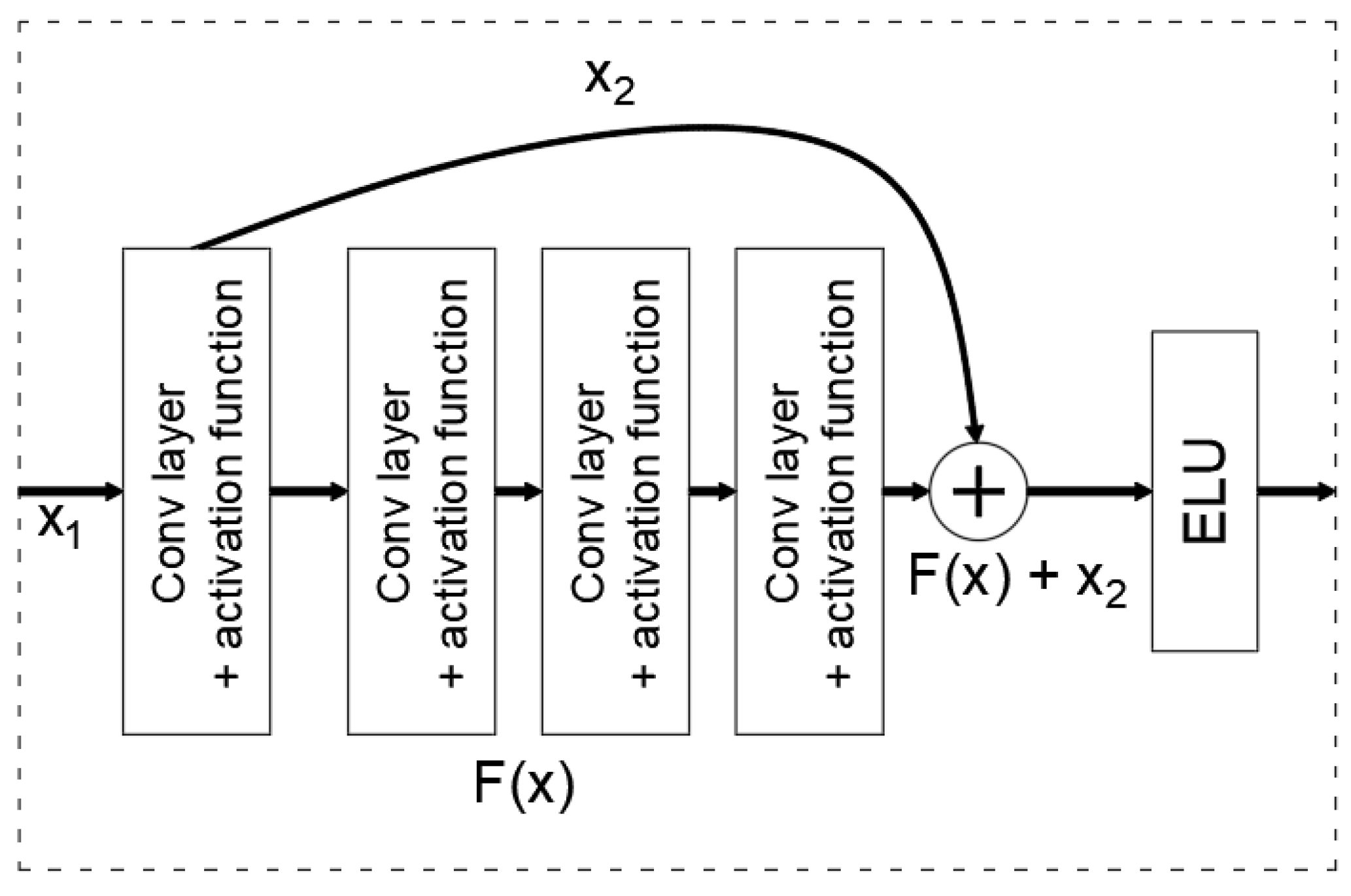
Architecture	Multi-branch encoder–decoder architecture	Multi-branch encoder–decoder architecture with skip connections in each branch.
Residual Connections	None	Includes residual connections in each branch, allowing for better gradient propagation and retention of essential input features during the reconstruction process.
Activation	ELU	LeakyReLU
Feature Branch Merging	Results from different columns are combined to obtain the final image reconstruction.	Feature maps from each of the three branches are merged into a single tensor, which is then transformed into image space using a common decoder module consisting of two convolutional layers.

below. The results of our network’s performance on satellite images indicate that the application of residual blocks significantly improves the quality of generated image inpaintings and achieves better results than generators without residual connections.

The block diagram of the proposed ResGMCNN is shown in Figure 3. Essentially, it consists of two models—a generator and a discriminator. The generator model is responsible for creating a new sample $x=g(z;{\Theta }^{\left(g\right)})$, while the task of the discriminator network is to determine whether the obtained sample comes from the training data or is created by the generator. This decision is represented as a probability value ($d(x;{\Theta }^{\left(g\right)})$) of membership x to the training dataset. The most popular (and at the same time, the simplest) way to train generative adversarial networks is a zero-sum game, where the function $\vartheta ({\theta }^{\left(g\right)},{\theta }^{\left(d\right)})$ has a major impact on the output of the discriminator network, while the generator model receives $-\vartheta ({\theta }^{\left(g\right)},{\theta }^{\left(d\right)})$ as a reward. During the training process, each player aims to maximise their reward, as represented by the formulas below (Equations (1) and (2)). The discriminator model presents a probability value based on $d\left(x,{\theta }^{\left(d\right)}\right)$, which indicates the probability that the evaluated image is real [56].

$$g*=\mathrm{a}\mathrm{r}\mathrm{g}{\mathrm{m}\mathrm{i}\mathrm{n}}_g{\mathrm{m}\mathrm{a}\mathrm{x}}_{d}v\left(g,d\right)$$

(1)

$$\vartheta ({\theta }^{\left(g\right)},{\theta }^{\left(d\right)})=E_{x~pdata} \mathrm{l}\mathrm{o}\mathrm{g}d\left(X\right)+E_{x~pmodel} \mathrm{l}\mathrm{o}\mathrm{g}d(1-d(x\left)\right)$$

(2)

The approach outlined above (Equations (1) and (2)) allows for stimulating the discriminator network to improve the classification of samples, while the generator aims to deceive the classifier.

In the ResGMCNN model (as well as in its predecessor GMCNN), two images are taken as input to the network—the original image and a mask (which is a binary image where fragments intended for reconstruction or masking take the value of 1) (Figure 3). Based on these, the generator model attempts to fill in the missing areas as accurately as possible so that they cannot be distinguished from the rest of the image. Subsequently, the generated image is evaluated using two discriminators—a local one (assessing the filled gaps in the image) and a global one (evaluating the entire image). The generator network consists of three parallel branches of encoder and decoder (Figure 4) to capture different levels of features from the input image and mask, along with a shared decoder module to transform deep features into the natural image space. For each branch of the generator, different receptive fields and spatial resolutions are chosen, allowing them to capture various levels of information—information is filled in, not inherited, as is the case with commonly used encoder–decoder models [41].

A single branch of the ResGMCNN generator can be divided into three main components: (1) convolutional layers using residual connections, (2) four convolutional layers with dilated kernels, and (3) layers responsible for restoring feature maps to their original sizes. Subsequently, the feature maps from each branch are merged into a single tensor, which is transformed into an image space using a decoding module consisting of two convolutional layers.

The introduction of a multi-branch structure in the ResGMCNN generator increases its complexity, making model training more challenging. However, in the task of image inpainting, this structure allows for the representation of features at different levels. Thanks to the multi-branch design of the generator, it is possible to simultaneously capture both global and local features, facilitating the alignment of generated fragments with the surrounding context. Each branch of the encoder and decoder operates on different receptive fields and spatial resolutions, enabling a more comprehensive reconstruction of missing areas in the image.

The use of residual connections introduces a mechanism in which the input tensor is added to the output of the network layers via a skip connection, eliminating the need for a complete transformation of data at each layer. This approach can be formally represented as Equation (3):

$$y=F\left(x,W\right)+x$$

(3)

where x denotes the input to the residual block, W represents the parameters of the transformation layers, and $\mathrm{F}\left(\mathrm{x},\mathrm{W}\right)$ is a nonlinear function learned by the network. The key advantage of this solution is that it allows the model to learn the identity function when necessary, which significantly impacts the generated results in the image reconstruction task. The residual connection mechanism is illustrated in the figure below (Figure 5). When residual connections are implemented, it becomes possible to incorporate the input data of a residual unit into the output data, which leads to the modelling of an identity function. This solution addresses several issues: (1) When training a classical neural network begins, its weights have small values, making the training process very time-consuming. If the target function is close to the identity function, the concatenation of the input data into the output data significantly accelerates the learning process. (2) The occurrence of the vanishing gradient problem or representation bottlenecks is considerably reduced when these connections are used.

By implementing residual connections, it is possible to merge input data with the output of the residual unit, significantly improving the stability and efficiency of learning. In classical neural networks, the challenge of deep learning arises from the fact that in the early stages of training, weight values are small, leading to very slow signal propagation and prolonging the optimisation process. When the target function is close to the identity function, the use of residual connections enables efficient gradient propagation, reducing the problem of vanishing gradients and improving learning stability. In the case of the ResGMCNN model, it is crucial that the model not only learns to represent global structures but also accurately reconstructs local image features, such as textures and edges. Residual connections support this process by allowing better information flow through successive network layers, preventing the degradation of important details. Additionally, this mechanism enables the modelling of long-range contextual dependencies, which positively affects the quality of the generated output images.

Similarly to GMCNN, the ResGMCNN model employs implicit diversified Markov random fields (ID-MRF) (only during the training phase as regularisation) to avoid overfitting. This approach allows for the reduction in discrepancies between the generated content and the nearest corresponding neighbours of real samples in the object space. A direct similarity measure is used to calculate the ID-MRF loss, allowing the identification of areas closest to neighbours for patches. The filled areas exhibit high diversity in filling, while the occurrence of homogeneous spots is significantly lower.

The ResGMCNN was trained on the basis of the aforementioned databases. All the necessary scripts were implemented using the Python 3.9 programming language. The Keras library was used to build the convolutional network. In all cases, the network was trained for 400 epochs using a computer equipped with an Intel Xeon Silver 256GB and an NVIDIA TITAN RTX 24 GB graphical processing unit (GPU). Its results are shown in the following figure (Figure 6). ResGMCNN achieved the best results for the training parameters: wgan training ratio = 5, batch size = 2, learning rate = 0.000005, adversarial loss weight parameters = 0.0008, and Gaussian kernel size = 32.

Removing Area Objects from Images

In this section, we describe the potential applications of inpainting to remove unnecessary surface objects that disrupt the homogeneity of classes in an image. This is illustrated by the example of removing cars from the road. The large number of vehicles on the road generates classification errors, which negatively impacts the accuracy of calculating the area covered by the roads. Removing vehicles from images will clean up the class of roads from errors, thus improving classification, which in turn will enhance the accuracy of the analyses based on this classification. Inpainting can be an effective method for cleaning image classes while maintaining their consistency and avoiding the introduction of additional errors into the image.

Inpainting allows one to conceal an object in an image using a combination of various image processing techniques. This process consists of two main stages: the creation of a mask and the replacement of pixel values of the objects covered by this mask. The effectiveness of inpainting depends on the method used, but primarily on how the mask is developed. The mask is a binary image where white pixels (value 1) represent the object to be removed, while black pixels (value 0) indicate the background that should remain unchanged during image processing. The mask should be designed so that the objects (to be removed from the background) are entirely covered by white pixels. Inaccuracy in this area results in an incomplete removal of the object from the image, leading to improper inpainting. The processed image may retain fragments of the removed objects or exhibit local blurring at the edges of these objects. Therefore, a key task is to develop a methodology for generating car masks. This mask serves as the basis for subsequent processing in the inpainting process. The method for generating the mask is illustrated in the diagram (Figure 7).

In the first step, only the road areas are selected from image I. This is a simple stage, yet it is crucial for the effectiveness of car mask generation. Cars in RGB images have very diverse spectral properties, which are seen as a variety of colours of vehicles on the road. Isolation of the roads from the surrounding environment depicted in the image minimises errors in car segmentation (in subsequent steps). Without this stage, the final car mask would contain misclassified pixels showing, among other things, the roofs of buildings or other objects with similar spectral properties that are outside the area of interest (roads). Defining roads as the region of interest (ROI) allowed an image segmentation to determine the road mask (BW_road). The road mask is a binary image where the pixels indicating the roads have a value of 1, while the remaining pixels have a value of 0. Subsequently, according to Equation (4), the image I_road was developed to show only the roads:

$${\mathit{I}}_{\mathit{r}\mathit{o}\mathit{a}\mathit{d}\left(\mathit{k}\right)}={\mathit{I}}_{\left(\mathit{k}\right)}·{\mathit{B}\mathit{W}}_{\mathit{r}\mathit{o}\mathit{a}\mathit{d}}$$

(4)

k denotes the channel of image I.

The resulting image I_road retains the properties of the input image within the ROI (Region of Interest). This means that when developing sets of RGB images, each resulting image I_road is also in the RGB range. The spectral properties of the roads and the objects visible on them remain unchanged.

In the next step, we perform semi-automatic segmentation of the I_road image to detect cars. First, the RGB image was converted to the L*a*b colour space. The L*a*b space is the best representation of colour perception by the human eye. L*a*b is a three-dimensional space, where the L axis describes the brightness of the colour. The a and b axes determine the proportion of the selected hue in the analysed colour. The a axis represents the proportion of hues from green to red, while the b axis represents the proportion of hues from blue to yellow [57]. Thus, the a and b axes contain chrominance information, so the use of the L*a*b space makes it possible to separate colour brightness from chrominance. Chrominance analysis allows a clearer separation of vehicles from the background (road) compared to the RGB colour space, resulting in a more effective selection of cars in the mask-making process. In the next step, a large sample base (around 300 background samples and about 800 vehicle samples) was identified in the UAV images. To achieve accurate segmentation, it was necessary to take into account the large variety of vehicle colours and details. These samples were selected to take into account the different brightness and chrominance of the vehicles and their shadows. Based on the determined samples, superpixels were calculated and presented in colours corresponding to those in the image in L*a*b space. The next step was to convert from L*a*b to the [0;1] range and the image segmentation to the background and foreground using a graph-based algorithm.

The result of the segmentation was a binary image BW_car, where white objects corresponded to cars, and black pixels indicated the background. Even with a very large number of samples, discontinuities can occur in the segmented objects (for example, caused by shadows, glass, or changes in light reflection on parts of the vehicle). In the inpainting, it is crucial that the mask completely covers the object to be removed. To ensure that each object was uniform, complete, and completely covered by the mask, mathematical morphology was applied. In most cases, because of shadows, the mask was incomplete at the edges of the cars. Consequently, dilation was used according to Equation (5).

$${\mathit{B}\mathit{W}}_{\mathit{c}\mathit{a}\mathit{r}-\mathit{f}\mathit{i}\mathit{n}\mathit{a}\mathit{l}}={\mathit{BW}}_{\mathit{car}}⨁\mathbf{E}=\{\left(\mathrm{x},\mathrm{y}\right)+(\mathrm{i},\mathrm{j}):(\mathrm{i},\mathrm{j})\in Q_{{\mathit{B}\mathit{W}}_{\mathit{c}\mathit{a}\mathit{r}}}, \left(x,y\right)\in Q_E \}$$

(5)

where BW_car-final represents the final mask for cars, $\mathbf{E}$ denotes the structural element, $(\mathrm{i},\mathrm{j})$ are the coordinates of the mask ${\mathit{B}\mathit{W}}_{\mathit{c}\mathit{a}\mathit{r}}$, and $\left(x,y\right)$ are the coordinates of the structural element $\mathbf{E}$.

Dilation allows the expansion of objects and fills in holes and peninsulas. The structural element was shaped like a circle with a radius of 15 pixels. The circular shape allowed the expansion of the car mask regardless of direction, while such a large radius ensured the complete filling of holes (for some cars, holes caused by glass exceeded 20 pixels). The product of this step was the final car mask BW_car-final, which was then used for inpainting. The white areas must completely cover the vehicles on the road, regardless of their shape and colour. The objects in the mask should also be cohesive and complete. There should be no holes in them. They should not be too small or narrow, as this would prevent them from fully covering the car, leading to inpainting errors, such as the partial reconstruction of the vehicle. Figure 8 shows the results of the development of the car mask according to our methodology. The mask is overlaid on the original image to verify its correctness. The white areas indicate the objects (cars) that are to be removed from the image.

As seen in the above figure (Figure 8), the vehicles on the roads are completely covered by white pixels of the mask. This means that in the inpainting process, they are completely removed from the image and replaced with pixels similar to their surroundings. The application of morphology on the images allowed for the complete masking of the vehicles. Segmentation enabled semi-automatic vehicle detection; however, the objects were not entirely covered by white pixels. Typically, part of the vehicle had a different colour saturation due to shadows. Furthermore, most cars in the UAV images have windows depicted by dark pixels, very similar to the pixels showing shadows. With a GSD of about 3 cm, such a window generates a spot of about several dozen pixels. Considering the spectral properties of these pixels in the segmentation introduced many falsely detected objects (such as shadows of trees and buildings). A better solution was to fill these gaps using morphological operations. The dilation expanded the objects so that the holes in the mask were filled. The shape and size of the structural element were chosen to ensure that each object could be fully complemented. Additionally, this operation eliminated the influence of car shadows on the inpainting effect. As a result, each vehicle on the road was accurately masked, which further allowed its complete removal from the image.

The research described in Section 4.1.1 allowed the selection of the best inpainting technique to reconstruct the image after the removal of cars. The best results, both visually and quantitatively, were achieved using the Criminisi method. Good results were also obtained with the Telea and Navier–Stokes methods. Methods based on GAN lead to greater blurring, and therefore they will not be effective for reconstructing cars on the road.

The inpainting was performed according to the Criminisi method. This method employs a “best-first” algorithm, where confidence in the synthesised pixel values is propagated similarly to information propagation in painting. Actual colour values are computed using pattern synthesis. The quality of the output image synthesis is significantly influenced by the order in which the filling process occurs. Combining the structure “push” with a confidence term provides a balance between the propagation of structural regions and textured regions without employing two strategies [9].

The inpainting process takes place in the source region, which is the image with the objects removed as designated by the mask. The source region is defined according to Equation (6):

$$\mathit{\varphi }=\mathit{I}-{\mathit{B}\mathit{W}}_{\mathit{c}\mathit{a}\mathit{r}-\mathit{f}\mathit{i}\mathit{n}\mathit{a}\mathit{l}}$$

(6)

Each pixel retains information about its RGB values and a confidence value. If a pixel requires filling, the information “empty” is preserved. The confidence value indicates the trust in the pixel values and is frozen after the pixel is filled. During the inpainting, empty pixels receive a temporary priority value that determines the order in which they are filled. The process then proceeds iteratively, repeating the following three steps [9]:

• Computing patch priorities.
• Propagating texture and structure information.
• Updating confidence values.

The iteration is complete when all the pixels are filled in. In the first step, the synthesis task is performed using a best-first filling strategy. This operation depends on the priority values of the pixels, which in turn are determined by their location on the continuation of strong edges and the surrounding pixels with high confidence according to Equation (7) [9]:

$$P(\mathrm{i},\mathrm{j})=C(\mathrm{i},\mathrm{j})D(\mathrm{i},\mathrm{j})$$

(7)

where $P(\mathrm{i},\mathrm{j})$ represents the priority value of the pixel with coordinates $(\mathrm{i},\mathrm{j})$, C(i,j) represents the confidence term, and $D(\mathrm{i},\mathrm{j})$ is a data term.

Priorities are calculated for all the pixels located on the borders of the objects to be filled. The confidence component C is a measure of the amount of reliable information surrounding the pixel. The more pixels that have already been filled, the higher the priority of the pixel. The data component D is a function of the strength of isophotes that impact the mask ${\mathit{B}\mathit{W}}_{\mathit{c}\mathit{a}\mathit{r}-\mathit{f}\mathit{i}\mathit{n}\mathit{a}\mathit{l}}$ in each iteration. If an isophote affects the area (group of pixels to be filled), the priority of that area increases. This factor influences the synthesis of linear structures first. After calculating all the priorities, the algorithm moves to the second step. The propagation of texture in the image occurs through the direct sampling of the source region, which helps avoid blurring of the image. In the source image I, an area most similar to the pixel with the highest priority (determined in the first step) is sought using the least squares method. In the third step, the confidence factor is updated. As the filling progresses, the confidence values decrease, indicating that the closer the centre of the filled area, the lower the certainty of the pixel values [9].

4.1.2. Results of the Inpainting

In this subsection, we present the results of inpainting on various remote sensing images. In the following points, we describe the following: (1) the results of removing linear objects from images and the application of the new ResGMCNN method; (2) the results of removing unnecessary surface objects from the background using the example of cars on the road.

Results of the ResGMCNN Algorithm

The prepared model was validated based on three databases: (1) DOTA—A Large-scale Dataset for Object Detection in Aerial Images [51]; (2) Cars Overhead With Context (COWC) [52]; and (3) our own database created from a satellite scene captured by WorldView-2 (using fragments depicting fields, meadows, and forests). For the study, the images were divided into smaller patches of size 256 × 256 pixels. Additionally, to reflect the occurrence of artefacts or areas that are to be masked in the images, a set of masks prepared by the NVIDIA Irregular Mask Dataset was used. The performance of the algorithm was compared with GMCNN that did not contain residual connections, GMCNN with the LeakyReLU activation function and with the Navier–Stokes method, A. Telea, and Criminisi.

In the case of panchromatic images (Figure 9A), the GMCNN [41] model presented by Y. Wang allows for the difficult-to-distinguish filling of missing areas. However, there are instances where the new, false images contain point artefacts that stand out in the images. For RGB images (Figure 9B), the results of this network’s performance are significantly worse—the filled areas differ greatly from the surroundings, making them easy to locate.

Before proceeding to modify the generator model, the impact of changing the training parameters and the network model on its performance was examined. However, as the following studies show, none of the changes positively affected the ability to generate lost areas of the images (Figure 10).

As the size of the Gaussian filter mask decreased, the filled areas became more varied but significantly different from the surroundings. Reducing the standard deviation of the mask caused image blurring. Decreasing the ratio parameter resulted in colour banding in the fillings.

To perform a qualitative analysis of the studied network, the structural similarity index measure (SSIM) was used to measure the similarity of images after applying the masking restoration to their original versions [58]. This index was checked for the test images of each of the studied databases, as well as for the GMCNN, GMCNN with Leaky ReLU, and ResGMCNNs. Additionally, these results were compared with the A. Telea, Navier–Stokes, and Criminisi algorithms (

Table 2. SSIM for masked images using the following methods: Navier–Stokes, Telea, GMCNN, GMCNN with Leaky ReLU, and ResGMCNN.

	Navier–Stokes	Telea	Criminisi	GMCNN	GMCNN with Leaky ReLU	ResGMCNN (our)
DOTA	0.803	0.804	0.982	0.675	0.708	0.905
WV2	0.929	0.815	0.988	0.769	0.719	0.931
COWC	0.913	0.911	0.994	0.864	0.846	0.925

).

The analysis of the results indicates that the classical Criminisi method achieves the highest effectiveness across all the datasets, obtaining scores of 0.982 for DOTA, 0.988 for WV2 and 0.994 for COWC. The Navier–Stokes and the Telea methods demonstrate comparable effectiveness, although their results are significantly lower than those of the Criminisi method, particularly for the DOTA and WV2 datasets. Among deep learning-based methods, GMCNN performs worse than ResGMCNN and GMCNN with the Leaky ReLU activation function, suggesting that architectural enhancements, such as the use of residual layers in ResGMCNN, significantly improve result quality. ResGMCNN, an original solution, achieves results close to classical methods, outperforming GMCNN in all the datasets, especially for DOTA (0.905) and WV2 (0.931). The results indicate that the application of improved network architectures allows a significant enhancement in image inpainting, although classical methods still dominate in terms of effectiveness for tasks requiring very high accuracy.

Given the superiority of classical inpainting methods in aerial and satellite data tests and their high effectiveness in reconstructing image structures, only classical methods will be utilised for further research.

Results of Removing Cars from Images

The proposed approach to remove cars from images was based on inpainting using the Criminisi method, which is an effective patch-based method. For comparison, two popular diffusion-based methods, Telea and Navier–Stokes, were also employed. All the used methods are popular, traditional sequential-based methods that are or can be easily implemented in various image processing environments. The results of the car inpainting using the aforementioned methods are shown in the figures (Figure 11).

In visual assessment, it is easy to observe that the Criminisi method yields the best results. Unlike the Telea and Navier–Stokes methods, the image after reconstruction does not exhibit blurred patches. The cars are removed, and their locations are smoothly filled with pixels that have the same (or very similar) properties as the road pixels. There are no artificial boundaries of objects in the reconstructed images, and the locations of the vehicles that were removed cannot be recognised. This is undoubtedly a significant advantage of this method. Unfortunately, the other methods introduced errors into the image, primarily blurring the edges of the filled areas (Figure 12).

Figure 12 shows that some commonly used inpainting methods (such as Navier–Stokes and Telea) are not suitable for car removal from UAV images. The cars are removed but artificial patches have formed in their place. This is detrimental for further processing, as road classification in such an image will still be inaccurate and the roads will not be coherent objects. Inpainting using the Criminisi method does not cause blurring in the image and the objects are reliably reconstructed. The continuity of curbs, lanes on the road and, most importantly, the road itself is preserved. In areas of image reconstruction, there are no discolourations that could negatively affect the quality of road classification. Figure 12 also shows an example of shadow reconstruction. The figure shows a white car in the shadow of a tall tree. The Navier–Stokes and Telea methods caused blurring in the reconstructed part of the shadow, making it have an altered and unnatural shape. The Criminisi method uses texture synthesis and the best-first algorithm during gap filling, and therefore the shadow is reconstructed better here. Its shape is preserved, without blurring. However, all the methods have their limitations, so some fine details may not be reproduced. Texture propagation is based on full pixel analysis, so it is not always possible to reproduce the actual shape. Nevertheless, the Criminisi method is quite effective in predicting reconstructed objects.

We verify the visual quality assessment of the images using specific metrics. Due to the lack of a reliable reference image, no reference metrics were used. Obtaining a reference image under real-world conditions is practically impossible, especially in areas with heavy traffic. Even if it were possible to take a picture of a road without vehicles, it would certainly be captured with different exposure parameters. This, in turn, would result in a different image quality for the same area [59]. Therefore, the following metrics were used to assess image quality: Perception-based Image Quality Evaluator (PIQE), Natural Image Quality Evaluator (NIQE), No-Reference Perceptual Blur Metric (NRPBM), and Entropy. PIQE relies on the extraction of local features to predict quality. Quality is assessed only from spatial regions that are perceptually relevant, but at the same time, PIQE does not require supervised learning [60]. NIQE uses only measurable deviations from statistical regularities observed in natural images without training on distorted images evaluated by humans, or even without any exposure to distorted images [61]. The higher the NIQE and PIQE values, the worse the image quality. To assess image blurring, we used NRPBM, which is based on distinguishing different levels of blurriness perceptible in the same image [61]. NRPBM takes values ranging from 0 to 1, which characterise the best and worst image quality in terms of blurriness, respectively [62]. Additionally, Entropy was also calculated, which is a measure of the information contained in the image. The higher the Entropy value, the more information the image carries.

Table 3. Assessment of the quality of the original image and images after inpainting.

Radom
Metric/image	original	Criminisi	Navier–Stokes	Telea
PIQE	30.282	25.538	27.917	27.310
NIQE	1.876	2.504	2.506	2.502
NRPBM	0.267	0.257	0.262	0.262
Entropy	7.677	7.665	7.658	7.657
Warsaw
Metric/image	original	Criminisi	Navier–Stokes	Telea
PIQE	26.005	25.264	27.073	26.743
NIQE	1.988	1.987	2.023	1.998
NRPBM	0.263	0.262	0.264	0.263
Entropy	7.517	7.515	7.512	7.513

summarises the averaged results for the set of images obtained for the regions of Radom and Warsaw.

The indicators confirm the conclusions of the visual analysis. Each inpainting method introduces changes to the image, resulting in slightly worse outcomes for the processed images compared to the original. However, among the used inpainting methods, the Criminisi method yielded the best results. The only exception is the NIQE value for the Radom image set, which is the lowest after using the Telea method, and this is a minor difference (only 0.002). In the other cases, the PIQE and NIQE metrics have the lowest values after applying the Criminisi method. Similarly, NRPBM indicates that the least blurring occurred in the image reconstructed using the Criminisi approach. For the Navier–Stokes and Telea methods, the NRPBM values are very similar, suggesting that they introduce blurring to the image at a comparable level. Meanwhile, the Entropy shows only slight variations between the methods, indicating a similar number of vehicles removed. This holds true, as the same masks were used in each approach and the same vehicles were painted. Only differences arose in the manner and accuracy of this painting. The Criminisi method allowed complete vehicle removal, whereas the Navier–Stokes and Telea methods did not completely remove the edges of some cars and the blur remained there. The Entropy analysis also shows that a larger change compared to the original image occurred in the Radom dataset. As mentioned above, the flight was conducted over an expressway that traversed the city centre. This is a segment of a very busy road, so many vehicles were visible in the images. Their removal significantly impacted the information content of the image, which was confirmed by the Entropy. In the case of the Warsaw dataset, difference is not as pronounced, as the flight was conducted over an area of allotment gardens, where the number of cars was relatively smaller.

4.1.3. Conclusions of the Inpainting

The results show that the use of a multi-column generator leads to a significant improvement in filling in missing parts of images, such as erroneous lines in the image. Although modern approaches utilising deep neural networks (ResGMCNN) demonstrate clear advancements in reconstruction quality, they still fall short in effectiveness compared to some classical inpainting methods in tasks requiring very high precision. For this reason, the methodology for removing real objects from the background (using cars as an example) was based on the Criminisi method, which produced the best results among the classical approaches studied. The results presented in Table 1 and Table 2 confirm the choice of this method.

The results of the quality assessment of the images after car inpainting (both by the visual method and using metrics) confirm that it was a good assumption to use the Criminisi method to remove cars from the road images in our proposed approach to improving the quality of the road classification (Table 3). The use of other traditional methods, especially those in the diffusion-based group, also allows for the inpainting of vehicles; however, it may adversely affect classification results.

4.2. Classification

In this section, we describe our research on classification in images before and after inpainting. Section 4.2.1 describes the used classification methods. Section 4.2.2 presents the classification results using various methods on images before and after inpainting. In Section 4.2.3, the key conclusions from the previous part of the experiment are summarised.

4.2.1. Methods of Classification

In this research, we used popular and classical classification methods. Additionally, we compared them with machine learning-based methods and proposed our own solutions.

We verified the impact of the applied inpainting on classification quality for several methods. Among the classical supervised classification methods, we utilised Maximum Likelihood (Figure 13a) and Mahalanobis Distance-Based Classification (Figure 13b), which exploit statistical dependencies between classes. KNN (k-nearest neighbours) (Figure 13c) [63] classifies objects based on similarity to the k-nearest neighbours, while Support Vector Machine (SVM) (Figure 13d) [64] defines a hyperplane that separates the classes. With the development of machine learning methods, more advanced techniques have emerged, such as Random Forest (RF) [65] (Figure 13e) and Gradient Boosting Classifier (GBC) [66] (Figure 13f), which are based on decision trees. RF creates a set of random trees (Figure 13e) and the GBC iteratively corrects errors from previous trees (Figure 13f). Gaussian Naive Bayes (GNB) [67] assumes a normal distribution of features and their independence (Figure 13g), while Multi-Layer Perceptron (MLP), as a neural network, learns nonlinear dependencies through backpropagation, providing greater flexibility in modelling complex data (Figure 13h).

Each of the described data classification methods operates differently. These differences are most evident in Figure 13, which presents the results of the RGB image classification after reduction in dimension using Principal Component Analysis (PCA) with machine learning methods. The goal of applying PCA was to reduce the number of dimensions of the input data while retaining as much relevant information for classification as possible. Since the original data had three features (RGB channels), their direct visualisation in a way that allows for an intuitive understanding of the structure and separability of classes would be challenging. Therefore, dimensionality reduction was applied to the two principal components of the PCA, allowing the representation of the data in a two-dimensional plot. The graphs visible in Figure 13 illustrate the division of space, where the first and second PCA components serve as the axes of the coordinate system, and the different colours represent various object classes, such as asphalt, concrete, shadows, soil, vegetation and buildings.

Dimensionality reduction using PCA allowed the mapping of data in a two-dimensional space, where the structure of the dataset and the decision boundaries of the classifier can be discerned. The first PCA component accounts for the greatest variance in the data, while the second retains the next most important information about the distribution of objects.

Analysing the plots, it can be observed that some classes, such as vegetation and soil, occupy relatively well-defined regions of the PCA space, while others, such as asphalt and shadows, overlap. This indicates similarities in their features, which may lead to classification difficulties. Figure 13a–h show the differences in data classification using various machine learning methods. It is evident that the models faced significant challenges in classifying data with low separability, particularly the SVM classifier.

Based on these graphs, it can be inferred that for classifying RGB images into the six considered classes, the k-NN model is likely to yield the best results, as its decision boundaries exhibit an irregular shape. This suggests that the k-NN classifier adapts to the local structure of the data. At the same time, areas can be observed where points belonging to different classes are close together, indicating the potential to generate misclassifications. Nevertheless, it can be expected that the number of errors will be lower than with the other machine learning methods.

As part of the conducted research, six machine learning models were prepared, designed to classify RGB images: k-nearest neighbours (KNN), Support Vector Machine (SVM), Random Forest (RF), Gradient Boosting Classifier (GBC), Gaussian Naive Bayes (GNB) and Multi-Layer Perceptron (MLP) (

Table 4. Best model parameters.

Model	Parameter	Image 1	Image 2	Image 3	Image 4
kNN	neighbours	7		5	5
	weights	distance *	Distance *	distance *	Distance *
SVM	kernel	RBF **	RBF **	RBF **	RBF **
	C	1.5	2.0	4.5	2.0
RF	max depth	20	20	20	None ***
	number of trees		200	50	200
GBC	learning rate	0.2	0.2	0.2	0.2
	max depth	7	7	7	5
	estimators	200	200	200	200
GNB	variance	1 × 10−9	1 × 10−9	1 × 10−9	1 × 10−9
MLP	activation	tanh	tanh	tanh	tanh
	layer sizes	(50,50)	(50,50)	(50,50)	(50,50)
	optimiser (solver)	Adam	Adam	Adam	Adam
	learning rate (init)	0.001	0.001	0.001	0.001

* Minkowski distance; ** radial basis function; *** if none, then nodes are expanded until all the leaves are pure or until all the leaves contain less than min_samples_split samples.

). Masks that were previously prepared during the verification of classical classification methods were used for their preparation. This enables a comparative analysis of all the verified methods. The image fragments bounded by the masks serve as input data for the models.

Classifiers were prepared based on RGB data, allowing the utilisation of all the information contained in the images. The aforementioned PCA dimensionality reduction was used solely to visualise the classification results obtained using different methods (which facilitates a better understanding of the methods).

The models were designed for four sample images obtained from flights 1 and 2. Images 1 and 4 were collected during flight 1, while images 2 and 3 were obtained during flight 2. The parameters of each model were carefully selected, taking into account the optimisation of their performance based on tuning methods such as GridSearchCV. This process allowed the adjustment of hyperparameters to achieve the best possible classification results, in line with the characteristics of the data under consideration. As a result, it was ensured that these models operate at maximum efficiency while minimising the risk of overfitting or underfitting.

To more accurately compare the effectiveness of machine learning models, the results obtained from their application were juxtaposed with the classification results achieved using traditional methods. For this purpose, six different models were prepared for each image, using masks created for classification with classical methods as training data. This allowed the establishment of a benchmark that enabled comparisons between the effectiveness of modern machine learning techniques and classical image classification methods.

4.2.2. Results of Classification

In the following sections, we describe the following: (1) the metrics used to assess the quality of classification; (2) the impact of removing unnecessary surface objects on the quality of classification, exemplified by the removal of cars and the classification of roads.

Metrics to Assess Classification Quality

To evaluate the effectiveness of the performed classification, commonly used indicators in the remote sensing environment were used. The most important among them include: confusion matrix, accuracy, precision, recall, F1-score, Jaccard index (Intersection over Union—IoU), and Cohen’s kappa coefficient. Each of these indicators provides a different perspective on the quality of classification and their values help to understand what errors were made by the classification algorithms. These metrics are described in

Table 5. Indicators for assessing segmentation quality.

Metric	Description	Goal
Accuracy	Accuracy is the ratio of the number of correctly classified samples to the total number of samples. It expresses the overall effectiveness of the classification algorithm. $\mathit{A}\mathit{c}\mathit{c}\mathit{u}\mathit{r}\mathit{a}\mathit{c}\mathit{y}={\displaystyle \frac{\mathit{T}\mathit{P}+\mathit{T}\mathit{N}}{\mathit{T}\mathit{P}+\mathit{T}\mathit{N}+\mathit{F}\mathit{P}+\mathit{F}\mathit{N}}}$ In the case of unbalanced datasets, where one class dominates, accuracy alone can be misleading.	1
Precision	Precision is a measure that indicates how many of the predicted positive examples are actually positive. $\mathit{P}\mathit{r}\mathit{e}\mathit{c}\mathit{i}\mathit{s}\mathit{i}\mathit{o}\mathit{n}={\displaystyle \frac{\mathit{T}\mathit{P}}{\mathit{T}\mathit{P}+\mathit{F}\mathit{P}}}$ High precision means that the model rarely misclassifies negative examples as positive.	1
Recall	Recall measures how many actual positive examples were correctly detected by the model. $\mathit{R}\mathit{e}\mathit{c}\mathit{a}\mathit{l}\mathit{l}={\displaystyle \frac{\mathit{T}\mathit{P}}{\mathit{T}\mathit{P}+\mathit{F}\mathit{N}}}$ High recall indicates that the model rarely misses positive cases.	1
F1-score	The F1-score is the harmonic mean of precision and recall. It is particularly useful in cases of imbalanced data (i.e., when one class occurs significantly more frequently than the other). $\mathit{F}1=2·{\displaystyle \frac{\mathit{P}\mathit{r}\mathit{e}\mathit{c}\mathit{i}\mathit{s}\mathit{i}\mathit{o}\mathit{n}·\mathit{R}\mathit{e}\mathit{c}\mathit{a}\mathit{l}\mathit{l}}{\mathit{P}\mathit{r}\mathit{e}\mathit{c}\mathit{i}\mathit{s}\mathit{i}\mathit{o}\mathit{n}+\mathit{R}\mathit{e}\mathit{c}\mathit{a}\mathit{l}\mathit{l}}}$	1 (perfect agreement) 0.8–1 (good agreement)
Indeks Jaccarda (Intersection over Union—IoU)	The Jaccard Index is a measure of the overlap between two sets, in this case, the classified image and the reference image. It is the ratio of the intersection of two areas to their union. $IoU={\displaystyle \frac{\left|A\cap B\right|}{\left|A\cup B\right|}}$ $\mathrm{where} \mathrm{A}—\mathrm{classified} \mathrm{pixels}, \mathrm{B}—\mathrm{true} \mathrm{objects} \mathrm{in} \mathrm{the} \mathrm{image}, \left|\mathit{A}\cap \mathit{B}\right|$$\mathrm{represents} \mathrm{the} \mathrm{number} \mathrm{of} \mathrm{pixels} \mathrm{that} \mathrm{have} \mathrm{been} \mathrm{correctly} \mathrm{classified} (\mathrm{i}.\mathrm{e}., \mathrm{present} \mathrm{in} \mathrm{both} \mathrm{sets} \mathrm{A} \mathrm{and} \mathrm{B}), \left|\mathit{A}\cup \mathit{B}\right|$ is the number of pixels classified as object or background in at least one of the images. A high IoU value indicates that the model’s classification closely matches the reference image.	1
Cohen’s Kappa	Cohen’s kappa measures the agreement between two classifications, accounting for the possibility of random agreement. $\mathit{\kappa }={\displaystyle \frac{2·(\mathit{T}\mathit{P}·\mathit{T}\mathit{N}-\mathit{F}\mathit{N}·\mathit{F}\mathit{P})}{\left(\mathit{T}\mathit{P}+\mathit{F}\mathit{P}\right)·\left(\mathit{F}\mathit{P}+\mathit{T}\mathit{N}\right)+(\mathit{T}\mathit{P}+\mathit{F}\mathit{N})·(\mathit{F}\mathit{N}+\mathit{T}\mathit{N})}}$ It is a useful metric when a classifier may accidentally classify images in agreement with the reference.	1 (perfect agreement) 0.8–1 (good agreement)

.

Results of the Classification After the Removal of Cars

In this article, we investigate whether inpainting could be applied to enhance the quality of image classification in remote sensing. The study was carried out using the example of the removal of cars from roads, with the aim of improving the classification of these roads. As previously described, the GAN-based methods resulted in more blurriness than the classical methods; therefore, we recommend using the Criminisi method for vehicle removal. Additionally, the same inpainting was performed for comparison using the Navier–Stokes and Telea methods. Cars were removed from each tested image using these three methods. Subsequently, classification was performed on these images before and after inpainting using various methods. Each version of the image was classified on the basis of the same set of samples. Each resulting image was analysed and metrics were calculated to assess the quality of the classification. The metrics were computed for both the entire images and individual classes. The objective of our research was to demonstrate the impact of inpainting on the quality of road classification, so the following charts (Figure 14) show the results of the quality assessment of road class classification before and after inpainting using different methods. These are the average values of the images analysed from both UAV flights.

It is noticeable that the metrics for the original image have lower values than those for images with inpainted cars, indicating that the inpainting positively influences the improvement in the quality of the road classification. Only in the case of the accuracy metric did the inpainting result in a change of less than 1%, but it should be noted that this metric is sensitive to the ratio of class sizes relative to each other. This metric will be very sensitive to the mutual overlap of the shadow and asphalt classes. The shadow class introduced additional complications in the analyses, as there was often a dilemma about whether a given object should be classified as a road or a shadow. On the other hand, excluding the shadow class significantly reduced the quality of classification, as many dark objects were misclassified. At the same time, it is essential to recognise that shadows in aerial and BSP images are entirely natural and unavoidable. Such a problem will occur in every analysed photo with varying degrees of intensity.

For the remaining metrics, changes are on the order of several or even dozens of percent. Analysis shows that the best results were achieved for SVM classification. Metric changes range from about 6% for F1-score to around 13% for recall. It should be noted that the F1-score is recommended when one class occurs significantly more frequently than the other, which lends a certain “objectivity” to this metric, thereby allowing these results to have a higher level of trust. In the case of classical popular classifiers (Maximum Likelihood and Mahalanobis Distance), the classification quality metrics after inpainting increase from 1% (precision, Mahalanobis Distance, and Telea inpainting) to 6% (recall, Maximum Likelihood, and Criminisi inpainting). Other machine learning-based classifiers classified the images more accurately. Consequently, the inpainting also had a stronger impact on classification quality, resulting in metric improvements of up to 13% in comparison to the classification of the original image. Analysing the maximum metric values also reveals that for the original image (before processing), they are significantly lower than after applying any of the inpainting methods.

In the context of comparing various classification methods, it can be observed that the lowest classification quality was achieved using the SVM and GNB methods, while the best results were obtained with the kNN, RF and GBC methods. For example, the average Cohen’s kappa index was 0.393, 0.394, and 0.397, respectively. When analysing each image separately, the maximum Cohen’s kappa value reached 0.699, 0.696, and 0.698 for kNN, RF, and GBC, respectively. The difference between the average and maximum values arises from the varied characteristics of the images. Some images were more difficult to classify because of significant object overlap and class intermingling (such as the road and shadow classes), which introduced errors in the unambiguous assignment of pixels to classes.

When comparing different inpainting techniques, it is noticeable that all of them similarly improved the quality of road classification. The average metric values presented in the graphs are comparable across the different inpainting methods. Differences in classification quality improvement for successive inpainting methods generally do not exceed 1%. However, a detailed analysis of each dataset reveals that the Criminisi method often yields slightly better results than the others. For example, for the images from Flight 1, the F1-score reaches its highest value when using Criminisi inpainting for 75% of the classification results. This includes images where improvement occurs in every classification case, as well as instances where the Criminisi method outperformed the others in four cases, while the Telea method was superior in another four. For images from Flight 2, the effectiveness of the inpainting methods examined was comparable. Flight 2 featured a greater presence of shadows in the asphalt class, which unfortunately may have reduced the accuracy of the analyses. As mentioned earlier, the shadows often overlapped with the roads, causing inaccuracies in class determination. However, visual analysis indicates the superiority of the Criminisi method due to significantly less blurring in the area of the car masks. The Navier–Stokes and Telea methods left more blurring in the painted areas, negatively impacting classification quality (as confirmed by the image quality metrics described in Section Results of Removing Cars from Images). Sometimes, the blurred areas were classified by the algorithm as a class other than asphalt. After applying Criminisi inpainting, no other classes were classified on the road (except for shadows). Examples of classification before and after inpainting for one selected classification method (GBC) are shown in Figure 15.

Masking the cars on the road allowed a more accurate determination of the asphalt class, i.e., the road. Inpainting facilitated the removal of unnecessary objects that disrupted the coherence and uniformity of the class, thus resulting in greater alignment of the class with the ground truth. The results varied only slightly for individual images, with differences arising from the diverse characteristics of the images. The best results were obtained for the images from Flight 1, as they contained fewer shadows.

In Appendix A, the classification results using various methods for the image from Flight 1 after the Criminisi inpainting are compiled. This technique allowed the almost complete removal of cars from the roadway and enhanced the coherence of the asphalt class. Regardless of the variety of classification methods, the effectiveness of inpainting in improving the quality of road classification is evident. Despite the removal of cars, some methods (such as Mahalanobis, kNN, or SVM) were able to reveal lanes on the roadway. This may be an advantage of these classification methods in some applications.

4.2.3. Conclusions of Clasification

We performed a classification of the images before and after the inpainting using eight classifiers. For six of them, we developed machine learning models for classifying RGB images: k-nearest neighbours, Support Vector Machine, Random Forest, Gradient Boosting Classifier, Gaussian Naive Bayes, and Multi-Layer Perceptron. The evaluation of classification quality was based on dedicated metrics: accuracy, precision, sensitivity, F1-score, Jaccard index (IoU) and Cohen’s kappa coefficient. The greatest improvement in classification was achieved for the SVM classification, where metric changes ranged from about 6% for the F1-score to around 13% for recall in relation to the classification of the image before inpainting. Furthermore, considering the various inpainting techniques, it can be observed that all similarly improved the quality of road classification. Masking cars allowed a more accurate determination of the class of roads. Inpainting enabled the removal of unnecessary objects that disrupted the coherence and uniformity of the class, thereby increasing the class’s alignment with the ground truth.

5. Discussion

Inpainting was initially a technique primarily used in graphics. In recent years, research and publications have emerged regarding the application of inpainting in remote sensing for tasks such as: filling in missing data (mainly clouds [44,45]), texture and structure reconstruction, and improving image analysis quality [43]. We examined how inpainting affects the reduction in erroneous lines in images and the quality of classification. Moreover, in remote sensing, most of the applications of inpainting involve the reconstruction of an area covered by thick clouds [46,47,48,49,50]. Whereas we focused on removing and painting over vehicles that are on the road. Techniques for cloud mask generation cannot be used to detect cars, because these objects have different properties. Vehicles have similar shapes, while clouds have irregular shapes. Clouds in images are generally white or very bright, so they have high brightness and low chrominance. Cars, on the other hand, are very different objects in terms of their colour, so they primarily have different chrominances. Therefore, the detection of cars by semi-automatic segmentation required the identification of a large number of different samples. In addition, clouds are objects with homogeneous colour, surrounded by a diverse background. Cars are objects with different colours, surrounded by a homogeneous background (grey roadway). For this reason, other inpainting techniques can be effective for the reconstruction of areas covered by clouds and others for painting vehicles.

As part of our research, we conducted an analysis of one of the popular inpainting methods utilising GAN. We implemented the GMCNN model based on a multi-column generator, which is frequently used in the field of computer science for image reconstruction [68,69,70]. However, during our experiments, we noticed that this model generates numerous artefacts that are distinctly noticeable in images, particularly when reconstructing areas with complex structures.

Despite optimising training hyperparameters, we were unable to achieve satisfactory results in the task of inpainting fragments of satellite images, both panchromatic and RGB. In particular, the model struggled to reproduce textures and maintain realistic tonal transitions, resulting in visible artefacts. Ultimately, the trained GMCNN generator performed significantly worse compared to classical inpainting methods, as confirmed by subjective visual assessments and objective quality metrics.

In response to these limitations, we modified the generator by adding residual connections (ResGMCNN), which allow the transfer of information from earlier layers directly to the final layers through skip connections. This modification reduced the risk of vanishing gradient phenomena, improving the stability of the learning process, and enhancing the model’s ability to accurately reconstruct missing areas of the image.

This modification significantly improved the quality of the generated images, especially in the case of linear and point masks, which often appear in applications related to satellite image reconstruction. Moreover, the modified ResGMCNN model outperformed classical inpainting methods, except for the method by Criminisi, which still achieved the best results in terms of reconstruction accuracy.

Our research indicates that despite the growing popularity of deep learning-based methods, classical inpainting algorithms remain competitive, especially in the context of images obtained from low-altitude aerial and satellite sources. In particular, classical methods exhibit greater versatility as they do not require a time-consuming training phase and can be applied to images of any dimension without the need to adjust the model architecture. A comparison of classical methods and neural networks in the inpainting task is shown in

Table 6. Comparison of classical methods and neural networks in the inpainting task.

	Advantages	Disadvantages
Inpainting using deep learning (based on GMCNN and ResGMCNN)	- For ResGMCNN, better results than Telea and Navier–Stokes methods.	- High computational requirements during the training phase; - Time-consuming model training process—model susceptible to vanishing gradient phenomena; - Low learning rate (as a limitation of the vanishing gradient phenomenon) can generate artefacts or additional erroneous textures; - Limitations on the images to be processed (defined input size for the generator model).
Classical inpainting methods	- Does not require model training; - Low computational requirements; - Ability to process images of any size; - Easier interpretation of algorithm functioning.	- Telea and Navier–Stokes methods have worse results than GAN models with residual connections.

.

Classical inpainting methods, despite their simplicity, still provide competitive results, particularly in tasks requiring high reconstruction accuracy. Therefore, these methods were used for the subsequent part of the research. The Criminisi method gave particularly good results (on the basis of the SSIM analysis). This approach is based on pattern-based texture synthesis, so it is particularly effective in propagating regular patterns. The approach is effective for both linear structures and two-dimensional textures [9]. The road in the image has a uniform and regular texture, so the Criminisi method is effective in impainting objects on the road, and the SSIM index (which is a measure of structural similarity) reaches a high value.

The impact of inpainting on classification quality was examined through the example of removing cars from roads and verifying road classes. The combination of inpainting with road detection was also explored by Calimanut-Ionut Cira et al. [71], although they focused on the automatic extraction of roads from images. Our research demonstrated that inpainting can be applied to enhance the consistency and homogeneity of classes. An important stage preceding the inpainting is the accurate development of the car mask. We employed a combination of semi-automatic segmentation and image morphology for this purpose. This approach allowed sufficiently accurate masking of vehicles. Currently, many vehicle detection methods based on machine learning are being developed, which can also be used to create similar masks [45,72,73]. However, it is important to note that machine learning-based solutions are effective but require a very precise and time-consuming training process for the network, along with the prior preparation of large training and testing datasets. Some methods already developed are not suitable for UAV images, as they detect cars visible at an angle. Applying them to detect vehicles seen above would require retraining the network on a different dataset.

Our studies showed that Criminisi inpainting, although a classical method, is effective in removing cars from roads. Image quality indicators (PIQE, NIQE, and NRPBM) demonstrated that the least blur occurred in the reconstructed image using the Criminisi approach. The Telea and Navier–Stokes methods left a blurred image in the reconstruction area, similar to inpainting techniques based on GAN. The visual analysis of the reconstructed images also confirmed that the Criminisi method is more effective in concealing objects compared to the Telea or Navier–Stokes methods. The Criminisi method is designed for texture synthesis, so it is effective in reconstructing the background surrounding an object, especially if it is a uniformly textured background like a road. Texture propagation by directly sampling the source region avoids blurring the image. The Navier–Stokes and Telea methods belong to the diffusion-based methods group, so the empty region is smoothly filled from the border to the inside of the missing region. Both the fluid dynamics theory and the fast marching method are effective for small areas. For larger and irregular holes, where the texture varies in the near vicinity of the holes, they can cause some artefacts in the image. When painting cars on the roadway, there was blurring where the road surface next to the hole was varied or where there were shadows.

The experiment indicated that inpainting can be used to improve the quality of classification. The example of roads showed that removing unnecessary objects from the class (i.e., cars from the roadway) enables the development of a more coherent and consequently, more accurate class. In any given class, the elimination of unnecessary objects that disrupt class homogeneity will positively influence the quality of the classification. However, the roads most vividly reflect the problem of inconsistent classification due to the large number of diverse vehicles, especially in urban areas. This is exactly why we chose to conduct research on such an example. The results indicated that the quality of the classification could improve by several to over a dozen percent, depending on the metric, image, and classification method. The metrics more sensitive to class size discrepancies (such as accuracy) showed a lower percentage of change between the classification of the original image and that after inpainting. In contrast, the F1-score and Cohen kappa metrics indicated a more pronounced improvement, reaching up to 13% compared to the classification of the original image. Poorer results were achieved for images with many shadows cast on the roadway. In such cases, there was a problem in assigning points to the correct class, which affected classification quality. Furthermore, eight different classification methods were tested, which also yielded varying results. Each method classifies objects based on different assumptions, which naturally translate into the results. High values of classification quality metrics were achieved using the kNN, RF and GBC methods. The greatest improvement in classification quality was observed with the SVM method. The analyses were conducted by comparing the images obtained on two different flights. All the analyses confirmed that the application of inpainting improves the quality of road classification. Overall, the best results were achieved for the images transformed according to the Criminisi algorithm. However, there were also instances where greater improvements were observed after using the Navier–Stokes or Telea methods. Visual analysis confirms the greater effectiveness of the Criminisi method. However, each of the classical inpainting methods studied positively impacted the improvement in road classification quality. Our research demonstrated that classical inpainting methods can be employed to remove objects from images to improve their classification and subsequent analyses based on those images. Cleaned, uniform, and coherent classes will allow more accurate estimations of their area, for example.

6. Conclusions

In this work, we proposed a modification of the GMCNN generator. We demonstrated that the use of residual connections significantly improves the quality of filling in missing areas, as confirmed by the examples presented and the results. Further research is planned to develop a new architecture that will allow even more precise filling of hidden areas in satellite imagery.

In this paper, we proposed a modification of the GMCNN generator architecture by applying residual connections. Introducing this change enabled an increase in the model’s ability to propagate contextual information and more effective reconstruction of image structures in masked areas. We showed that this modification significantly improves the quality of reconstructing missing areas, as evidenced by both the obtained SSIM values and visual examples of reconstructed images. The GMCNN model with residual connections achieved better results than most classical inpainting methods, including the Telea and Navier–Stokes methods, obtaining SSIM values of 0.91 (DOTA), 0.93 (WV2), and 0.93 (COWC), respectively. However, despite the improvement in filling quality, these results still remain inferior to the Criminisi method, which achieved the highest SSIM values (0.98/0.98/0.99).

The results obtained indicate that classical inpainting methods, despite their simplicity, can still outperform deep learning-based methods in tasks requiring high reconstruction accuracy. This is particularly significant in the context of remote sensing imagery, where even minor errors in reconstructing structures can impact subsequent analyses, including object classification.

Additionally, while exploring potential applications of inpainting in processing remote sensing imagery, we conducted experiments on removing vehicles from roads and filling in missing image segments. The results suggest that accurate reconstructions of these areas contribute to improved classification effectiveness. Metrics such as the F1-score and Cohen kappa demonstrated an enhancement in classification quality of up to 13% compared to the original image classification. In most cases (with different images, classifiers, and metrics), the best results were achieved for images transformed according to the Criminisi algorithm. However, each of the classical inpainting methods studied positively influenced the quality of road classification. This indicates that the removal of obstructive objects can enhance the interpretation of remote sensing data, particularly in low-altitude imagery, where the presence of dynamic objects, such as vehicles, often complicates accurate terrain class recognition.

To eliminate cars from the roads, three popular classical inpainting methods were employed: Criminisi, Navier–Stokes, and Telea. The image quality indices (PIQE, NIQE, and NRPBM) achieved the best results for the images reconstructed using the Criminisi approach, which aligned with the visual analysis. The least blurring in the reconstruction area also occurred in the images processed with the Criminisi method.

Future research plans include expanding reconstruction methods to larger areas, where classical inpainting methods exhibit limitations and may generate artefacts. Furthermore, subsequent work will focus on the impact of various inpainting methods (both classical and deep learning-based) on classification results under different atmospheric conditions.

References

- Sun, Y.; Lei, L.; Li, Z.; Kuang, G. Similarity and Dissimilarity Relationships Based Graphs for Multimodal Change Detection. ISPRS J. Photogramm. Remote Sens. 2024, 208, 70–88. [Google Scholar] [CrossRef]
- Zheng, Z.; Ermon, S.; Kim, D.; Zhang, L.; Zhong, Y. Changen2: Multi-Temporal Remote Sensing Generative Change Foundation Model. IEEE Trans. Pattern Anal. Mach. Intell. 2025, 47, 725–741. [Google Scholar] [CrossRef] [PubMed]
- Jiang, W.; Sun, Y.; Lei, L.; Kuang, G.; Ji, K. Change Detection of Multisource Remote Sensing Images: A Review. Int. J. Digit. Earth 2024, 17, 2398051. [Google Scholar] [CrossRef]
- Goodfellow, I.; Pouget-Abadie, J.; Mirza, M.; Xu, B.; Warde-Farley, D.; Ozair, S.; Courville, A.; Bengio, Y. Generative Adversarial Nets. In Proceedings of the Advances in Neural Information Processing Systems, Montreal, QC, Canada, 8–13 December 2014; Curran Associates, Inc.: Red Hook, NY, USA, 2014; Volume 27. [Google Scholar]
- Zhang, X.; Zhai, D.; Li, T.; Zhou, Y.; Lin, Y. Image Inpainting Based on Deep Learning: A Review. Inf. Fusion 2023, 90, 74–94. [Google Scholar] [CrossRef]
- Agostinelli, F.; Anderson, M.R.; Lee, H. Adaptive Multi-Column Deep Neural Networks with Application to Robust Image Denoising. In Proceedings of the Advances in Neural Information Processing Systems, Lake Tahoe, NV, USA, 5–8 December 2013; Curran Associates, Inc.: Red Hook, NY, USA, 2013; Volume 26. [Google Scholar]
- Ciregan, D.; Meier, U.; Schmidhuber, J. Multi-Column Deep Neural Networks for Image Classification. In Proceedings of the 2012 IEEE Conference on Computer Vision and Pattern Recognition, Hongkong, China, 16–21 June 2012; pp. 3642–3649. [Google Scholar]
- Elharrouss, O.; Almaadeed, N.; Al-Maadeed, S.; Akbari, Y. Image Inpainting: A Review. Neural Process. Lett. 2020, 51, 2007–2028. [Google Scholar] [CrossRef]
- Criminisi, A.; Perez, P.; Toyama, K. Region Filling and Object Removal by Exemplar-Based Image Inpainting. IEEE Trans. Image Process. 2004, 13, 1200–1212. [Google Scholar] [CrossRef] [PubMed]
- Qin, Z.; Zeng, Q.; Zong, Y.; Xu, F. Image Inpainting Based on Deep Learning: A Review. Displays 2021, 69, 102028. [Google Scholar] [CrossRef]
- Shen, H.; Li, X.; Cheng, Q.; Zeng, C.; Yang, G.; Li, H.; Zhang, L. Missing Information Reconstruction of Remote Sensing Data: A Technical Review. IEEE Geosci. Remote Sens. Mag. 2015, 3, 61–85. [Google Scholar] [CrossRef]
- Harrison, P. A Non-Hierarchical Procedure for Re-Synthesis of Complex Textures. Monash University: Melbourne, Australia, 2000; p. 16. [Google Scholar]
- Jia, J.; Tang, C.-K. Image Repairing: Robust Image Synthesis by Adaptive ND Tensor Voting. In Proceedings of the 2003 IEEE Computer Society Conference on Computer Vision and Pattern Recognition, Madison, WI, USA, 18–20 June 2003; Volume 1, p. I-I. [Google Scholar]
- Zalesny, A.; Ferrari, V.; Caenen, G.; Gool, L.V. Parallel Composite Texture Synthesis. In Proceedings of the Texture 2002 Workshop-ECCV, Copenhagen, Denmark, June 2002; pp. 151–155. [Google Scholar]
- Jin, K.H.; Ye, J.C. Annihilating Filter-Based Low-Rank Hankel Matrix Approach for Image Inpainting. IEEE Trans. Image Process. 2015, 24, 3498–3511. [Google Scholar] [CrossRef]
- Guo, Q.; Gao, S.; Zhang, X.; Yin, Y.; Zhang, C. Patch-Based Image Inpainting via Two-Stage Low Rank Approximation. IEEE Trans. Vis. Comput. Graph. 2018, 24, 2023–2036. [Google Scholar] [CrossRef]
- Lu, H.; Liu, Q.; Zhang, M.; Wang, Y.; Deng, X. Gradient-Based Low Rank Method and Its Application in Image Inpainting. Multimed. Tools Appl. 2018, 77, 5969–5993. [Google Scholar] [CrossRef]
- Fan, Q.; Zhang, L. A Novel Patch Matching Algorithm for Exemplar-Based Image Inpainting. Multimed. Tools Appl. 2018, 77, 10807–10821. [Google Scholar] [CrossRef]
- Liu, J.; Yang, S.; Fang, Y.; Guo, Z. Structure-Guided Image Inpainting Using Homography Transformation. IEEE Trans. Multimed. 2018, 20, 3252–3265. [Google Scholar] [CrossRef]
- Zeng, J.; Fu, X.; Leng, L.; Wang, C. Image Inpainting Algorithm Based on Saliency Map and Gray Entropy. Arab. J. Sci. Eng. 2019, 44, 3549–3558. [Google Scholar] [CrossRef]
- Zhang, D.; Liang, Z.; Yang, G.; Li, Q.; Li, L.; Sun, X. A Robust Forgery Detection Algorithm for Object Removal by Exemplar-Based Image Inpainting. Multimed. Tools Appl. 2018, 77, 11823–11842. [Google Scholar] [CrossRef]
- Shen, H.; Zhang, L. A MAP-Based Algorithm for Destriping and Inpainting of Remotely Sensed Images. IEEE Trans. Geosci. Remote Sens. 2009, 47, 1492–1502. [Google Scholar] [CrossRef]
- Maalouf, A.; Carre, P.; Augereau, B.; Fernandez-Maloigne, C. A Bandelet-Based Inpainting Technique for Clouds Removal From Remotely Sensed Images. IEEE Trans. Geosci. Remote Sens. 2009, 47, 2363–2371. [Google Scholar] [CrossRef]
- Zhang, Q.; Lin, J. Exemplar-Based Image Inpainting Using Color Distribution Analysis. J. Inf. Sci. Eng. 2012, 28, 641–654. [Google Scholar]
- Wali, S.; Zhang, H.; Chang, H.; Wu, C. A New Adaptive Boosting Total Generalized Variation (TGV) Technique for Image Denoising and Inpainting. J. Vis. Commun. Image Represent. 2019, 59, 39–51. [Google Scholar] [CrossRef]
- Zhang, T.; Gelman, A.; Laronga, R. Structure-and Texture-Based Fullbore Image Reconstruction. Math. Geosci. 2017, 49, 195–215. [Google Scholar] [CrossRef]
- Hays, J.; Efros, A.A. Scene Completion Using Millions of Photographs. ACM Trans. Graph. 2007, 26, 4. [Google Scholar] [CrossRef]
- Li, H.; Luo, W.; Huang, J. Localization of Diffusion-Based Inpainting in Digital Images. IEEE Trans. Inf. Forensics Secur. 2017, 12, 3050–3064. [Google Scholar] [CrossRef]
- Sridevi, G.; Srinivas Kumar, S. Image Inpainting Based on Fractional-Order Nonlinear Diffusion for Image Reconstruction. Circuits Syst. Signal Process. 2019, 38, 3802–3817. [Google Scholar] [CrossRef]
- Telea, A. An Image Inpainting Technique Based on the Fast Marching Method. J. Graph. Tools 2004, 9, 23–34. [Google Scholar] [CrossRef]
- Bertalmio, M.; Bertozzi, A.L.; Sapiro, G. Navier-stokes, Fluid Dynamics, and Image and Video Inpainting. In Proceedings of the 2001 IEEE Computer Society Conference on Computer Vision and Pattern Recognition (CVPR 2001), Kauai, HI, USA, 8–14 December 2001; Volume 1, p. I-I. [Google Scholar]
- Bertalmio, M.; Sapiro, G.; Caselles, V.; Ballester, C. Image Inpainting. In Proceedings of the 27th Annual Conference on Computer Graphics and Interactive Techniques, New Orleans, LA, USA, 23–28 July 2000; ACM Press/Addison-Wesley Publishing Co.: Boston, MA, USA, 2000; pp. 417–424. [Google Scholar]
- Pathak, D.; Krahenbuhl, P.; Donahue, J.; Darrell, T.; Efros, A.A. Context Encoders: Feature Learning by Inpainting. In Proceedings of the 2016 IEEE Conference on Computer Vision and Pattern Recognition (CVPR), Las Vegas, NV, USA, 27–30 June 2016; pp. 2536–2544. [Google Scholar]
- Liu, G.; Reda, F.A.; Shih, K.J.; Wang, T.-C.; Tao, A.; Catanzaro, B. Image Inpainting for Irregular Holes Using Partial Convolutions. In Proceedings of the European Conference on Computer Vision (ECCV), Munich, Germany, 8–14 September 2018. [Google Scholar] [CrossRef]
- Yu, J.; Lin, Z.; Yang, J.; Shen, X.; Lu, X.; Huang, T.S. Free-Form Image Inpainting With Gated Convolution. In Proceedings of the International Conference on Computer Vision, Seoul, Republic of Korea, 27 October–2 November 2019; pp. 4471–4480. [Google Scholar]
- Nazeri, K.; Ng, E.; Joseph, T.; Qureshi, F.; Ebrahimi, M. EdgeConnect: Structure Guided Image Inpainting using Edge Prediction. In Proceedings of the IEEE/CVF International Conference on Computer Vision Workshops, Seoul, Republic of Korea, 27–28 October 2019; Available online: https://openaccess.thecvf.com/content_ICCVW_2019/html/AIM/Nazeri_EdgeConnect_Structure_Guided_Image_Inpainting_using_Edge_Prediction_ICCVW_2019_paper.html (accessed on 3 April 2025).
- Liu, Y.; Liu, C.; Zou, H.; Zhou, S.; Shen, Q.; Chen, T. A Novel Exemplar-Based Image Inpainting Algorithm. In Proceedings of the 2015 International Conference on Intelligent Networking and Collaborative Systems, Taipei, Taiwan, 2–4 September 2015; pp. 86–90. [Google Scholar]
- Yang, S.; Liang, H.; Wang, Y.; Cai, H.; Chen, X. Image Inpainting Based on Multi-Patch Match with Adaptive Size. Appl. Sci. 2020, 10, 4921. [Google Scholar] [CrossRef]
- Pu, C.; Song, R.; Tylecek, R.; Li, N.; Fisher, R.B. SDF-MAN: Semi-Supervised Disparity Fusion with Multi-Scale Adversarial Networks. Remote Sens. 2019, 11, 487. [Google Scholar] [CrossRef]
- Li, C.; He, K.; Liu, K.; Ma, X. Image Inpainting Using Two-Stage Loss Function and Global and Local Markovian Discriminators. Sensors 2020, 20, 6193. [Google Scholar] [CrossRef] [PubMed]
- Wang, Y.; Tao, X.; Qi, X.; Shen, X.; Jia, J. Image Inpainting via Generative Multi-Column Convolutional Neural Networks. In Proceedings of the Advances in Neural Information Processing Systems, Montreal, QC, Canada, 3–8 December 2018; Curran Associates, Inc.: Red Hook, NY, USA, 2018; Volume 31. [Google Scholar]
- Kuznetsov, A.; Gashnikov, M. Remote Sensing Image Inpainting with Generative Adversarial Networks. In Proceedings of the 2020 8th International Symposium on Digital Forensics and Security (ISDFS), Beirut, Lebanon, 1–2 June 2020; pp. 1–6. [Google Scholar]
- Zaytar, M.A.; El Amrani, C. Satellite Image Inpainting with Deep Generative Adversarial Neural Networks. IAES Int. J. Artif. Intell. IJ-AI 2021, 10, 121. [Google Scholar] [CrossRef]
- Czerkawski, M.; Upadhyay, P.; Davison, C.; Werkmeister, A.; Cardona, J.; Atkinson, R.; Michie, C.; Andonovic, I.; Macdonald, M.; Tachtatzis, C. Deep Internal Learning for Inpainting of Cloud-Affected Regions in Satellite Imagery. Remote Sens. 2022, 14, 1342. [Google Scholar] [CrossRef]
- Saxena, J.; Jain, A.; Krishna, P.R.; Bothale, R.V. Cloud Removal and Satellite Image Reconstruction Using Deep Learning Based Image Inpainting Approaches. In Proceedings of the Rising Threats in Expert Applications and Solutions; Rathore, V.S., Sharma, S.C., Tavares, J.M.R.S., Moreira, C., Surendiran, B., Eds.; Springer Nature: Berlin, Germany, 2022; pp. 113–121. [Google Scholar]
- Zhang, X.; Qiu, Z.; Peng, C.; Ye, P. Removing Cloud Cover Interference from Sentinel-2 Imagery in Google Earth Engine by Fusing Sentinel-1 SAR Data with a CNN Model. Int. J. Remote Sens. 2022, 43, 132–147. [Google Scholar] [CrossRef]
- Ma, X.; Huang, Y.; Zhang, X.; Pun, M.-O.; Huang, B. Cloud-EGAN: Rethinking CycleGAN From a Feature Enhancement Perspective for Cloud Removal by Combining CNN and Transformer. IEEE J. Sel. Top. Appl. Earth Obs. Remote Sens. 2023, 16, 4999–5012. [Google Scholar] [CrossRef]
- Li, J.; Lv, Y.; Xu, Y.; Weng, H.; Li, D.; Shi, N. Automatic Cloud Detection and Removal in Satellite Imagery Using Deep Learning Techniques. Trait. Signal 2024, 41, 857–865. [Google Scholar] [CrossRef]
- Zhou, H.; Wang, Y.; Liu, W.; Tao, D.; Ma, W.; Liu, B. MSC-GAN: A Multistream Complementary Generative Adversarial Network With Grouping Learning for Multitemporal Cloud Removal. IEEE Trans. Geosci. Remote Sens. 2025, 63, 1–17. [Google Scholar] [CrossRef]
- Jin, M.; Wang, P.; Li, Y. HyA-GAN: Remote Sensing Image Cloud Removal Based on Hybrid Attention Generation Adversarial Network. Int. J. Remote Sens. 2024, 45, 1755–1773. [Google Scholar] [CrossRef]
- Xia, G.-S.; Bai, X.; Ding, J.; Zhu, Z.; Belongie, S.; Luo, J.; Datcu, M.; Pelillo, M.; Zhang, L. DOTA: A Large-Scale Dataset for Object Detection in Aerial Images. In Proceedings of the IEEE Conference on Computer Vision and Pattern Recognition, Salt Lake City, UT, USA, 18–23 June 2018; pp. 3974–3983. [Google Scholar]
- Mundhenk, T.N.; Konjevod, G.; Sakla, W.A.; Boakye, K. A Large Contextual Dataset for Classification, Detection and Counting of Cars with Deep Learning. In Proceedings of the Computer Vision–ECCV 2016, Amsterdam, The Netherlands, 11–14 October 2016; Leibe, B., Matas, J., Sebe, N., Welling, M., Eds.; Springer International Publishing: Cham, Switzerland, 2016; pp. 785–800. [Google Scholar]
- Central Statistical Office Area and Population by Territory in 2022. Table 21 Area, Population and Locations by Commune. s.l. Central Statistical Office. Available online: https://stat.gov.pl/obszary-tematyczne/ludnosc/ludnosc/powierzchnia-i-ludnosc-w-przekroju-terytorialnym-w-2022-roku,7,19.html (accessed on 14 February 2025).
- Geoportal 2. Available online: https://polska.geoportal2.pl/map/www/mapa.php?mapa=polska (accessed on 30 January 2025).
- Drone for Fast and Accurate Survey Data Every Time. Available online: https://wingtra.com/ (accessed on 29 January 2025).
- Goodfellow, I.; Bengio, Y.; Courville, A. Deep Learning; MIT Press: Cambridge, MA, USA, 2016; ISBN 978-0-262-03561-3. [Google Scholar]
- Tkalcic, M.; Tasic, J.F. Colour Spaces: Perceptual, Historical and Applicational Background. In Proceedings of the IEEE Region 8 EUROCON 2003. Computer As a Tool., Ljubljana, Slovenia, 22–24 September 2003; Volume 1, pp. 304–308. [Google Scholar]
- Keelan, B. Handbook of Image Quality: Characterization and Prediction; CRC Press: Boca Raton, FL, USA, 2002; ISBN 978-0-429-22280-1. [Google Scholar]
- Sekrecka, A. Application of the XBoost Regressor for an A Priori Prediction of UAV Image Quality. Remote Sens. 2021, 13, 4757. [Google Scholar] [CrossRef]
- Venkatanath, N.; Praneeth, D.; Bh, M.C.; Channappayya, S.S.; Medasani, S.S. Blind Image Quality Evaluation Using Perception Based Features. In Proceedings of the 2015 Twenty First National Conference on Communications (NCC), Mumbai, India, 27 February–1 March 2015; pp. 1–6. [Google Scholar]
- Mittal, A.; Soundararajan, R.; Bovik, A.C. Making a “Completely Blind” Image Quality Analyzer. IEEE Signal Process. Lett. 2013, 20, 209–212. [Google Scholar] [CrossRef]
- Crete, F.; Dolmiere, T.; Ladret, P.; Nicolas, M. The blur effect: Perception and Estimation with a New No-Reference Perceptual Blur Metric. In Proceedings of the Human Vision and Electronic Imaging XII, San Jose, CA, USA, 29 January–1 February 2007; SPIE: Bellingham, WA, USA, 2007; Volume 6492, pp. 196–206. [Google Scholar]
- Fix, E.; Hodges, J.L. Discriminatory Analysis. Nonparametric Discrimination: Consistency Properties. Int. Stat. Rev. Rev. Int. Stat. 1989, 57, 238–247. [Google Scholar] [CrossRef]
- Vapnik, V.N. The Support Vector Method. In Proceedings of the Artificial Neural Networks—ICANN’97; Gerstner, W., Germond, A., Hasler, M., Nicoud, J.-D., Eds.; Springer: Berlin, Heidelberg, 1997; pp. 261–271. [Google Scholar]
- Ho, T.K. Random Decision Forests. In Proceedings of the Proceedings of 3rd International Conference on Document Analysis and Recognition, Montreal, QC, Canada, 14–15 August 1995; Volume 1, pp. 278–282. [Google Scholar]
- Friedman, J.H. Stochastic Gradient Boosting. Comput. Stat. Data Anal. 2002, 38, 367–378. [Google Scholar] [CrossRef]
- Bayes, T. An Essay towards Solving a Problem in the Doctrine of Chances. By the Late Rev. Mr. Bayes, F.R.S. Communicated by Mr. Price, in a Letter to John Canton, A.M.F.R.S. Philos. Trans. R. Soc. Lond. 1997, 53, 370–418. [Google Scholar] [CrossRef]
- Baracchi, D.; Boato, G.; De Natale, F.; Iuliani, M.; Montibeller, A.; Pasquini, C.; Piva, A.; Shullani, D. Toward Open-World Multimedia Forensics Through Media Signature Encoding. IEEE Access 2024, 12, 59930–59952. [Google Scholar] [CrossRef]
- Zhang, X.; Zheng, Z.; Gao, D.; Zhang, B.; Yang, Y.; Chua, T.-S. Multi-View Consistent Generative Adversarial Networks for Compositional 3D-Aware Image Synthesis. Int. J. Comput. Vis. 2023, 131, 2219–2242. [Google Scholar] [CrossRef]
- Rot, P.; Grm, K.; Peer, P.; Štruc, V. PrivacyProber: Assessment and Detection of Soft–Biometric Privacy–Enhancing Techniques. IEEE Trans. Dependable Secure Comput. 2024, 21, 2869–2887. [Google Scholar] [CrossRef]
- Cira, C.-I.; Kada, M.; Manso-Callejo, M.-Á.; Alcarria, R.; Bordel Sanchez, B. Improving Road Surface Area Extraction via Semantic Segmentation with Conditional Generative Learning for Deep Inpainting Operations. ISPRS Int. J. Geo-Inf. 2022, 11, 43. [Google Scholar] [CrossRef]
- Akshatha, K.R.; Biswas, S.; Karunakar, A.K.; Satish Shenoy, B. Anchored versus Anchorless Detector for Car Detection in Aerial Imagery. In Proceedings of the 2021 2nd Global Conference for Advancement in Technology (GCAT), Bangalore, India, 1–3 October 2021; pp. 1–6. [Google Scholar]
- Katar, O.; Duman, E. U-Net Based Car Detection Method For Unmanned Aerial Vehicles. Mühendis. Bilim. Ve Tasar. Derg. 2022, 10, 1141–1154. [Google Scholar] [CrossRef]