
MMTSCNet: Multimodal Tree Species Classification Network for Classification of Multi-Source, Single-Tree LiDAR Point Clouds


Abstract
1. Introduction
2. Materials and Methods
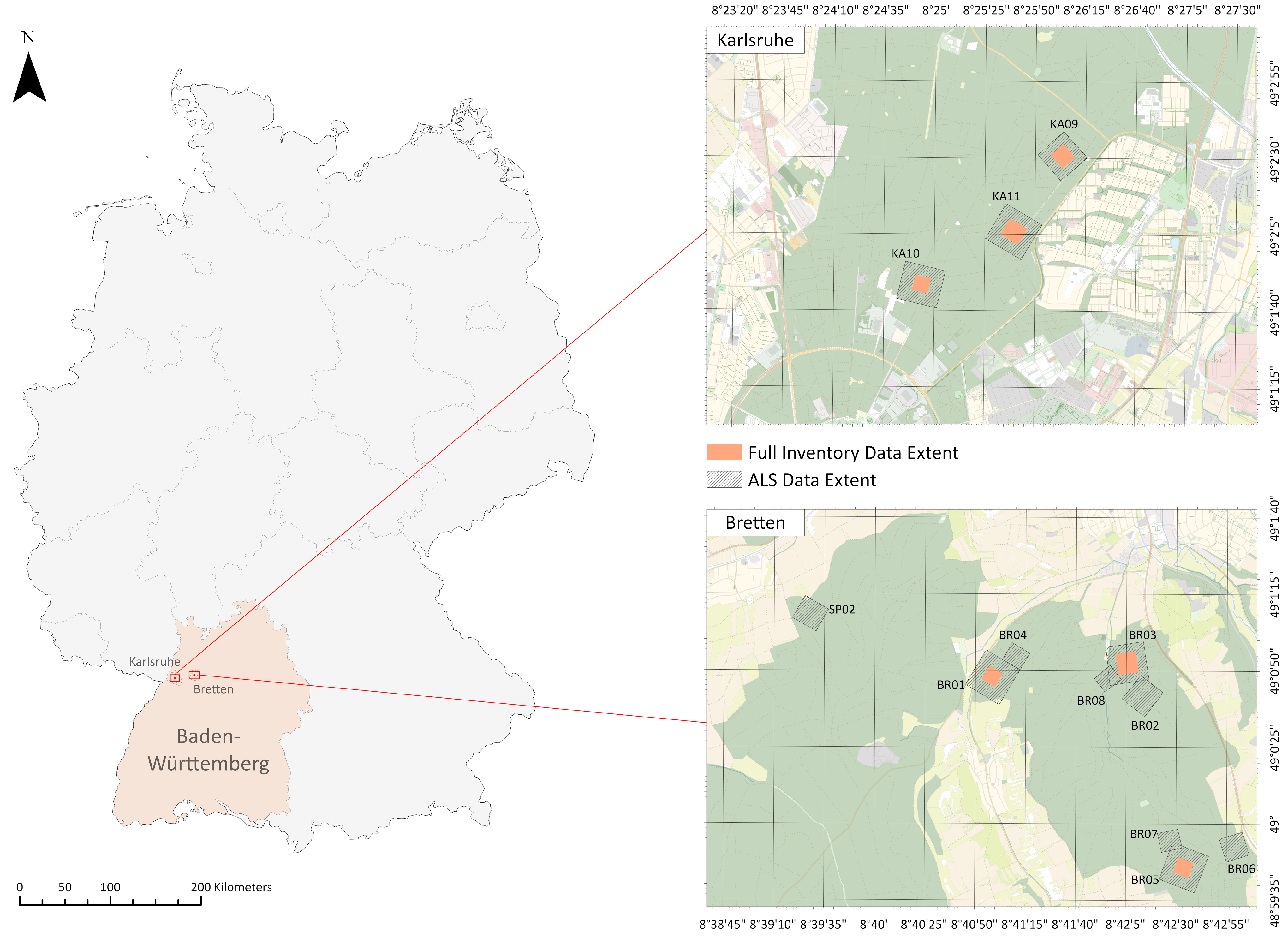
2.1. Study Sites and Datasets
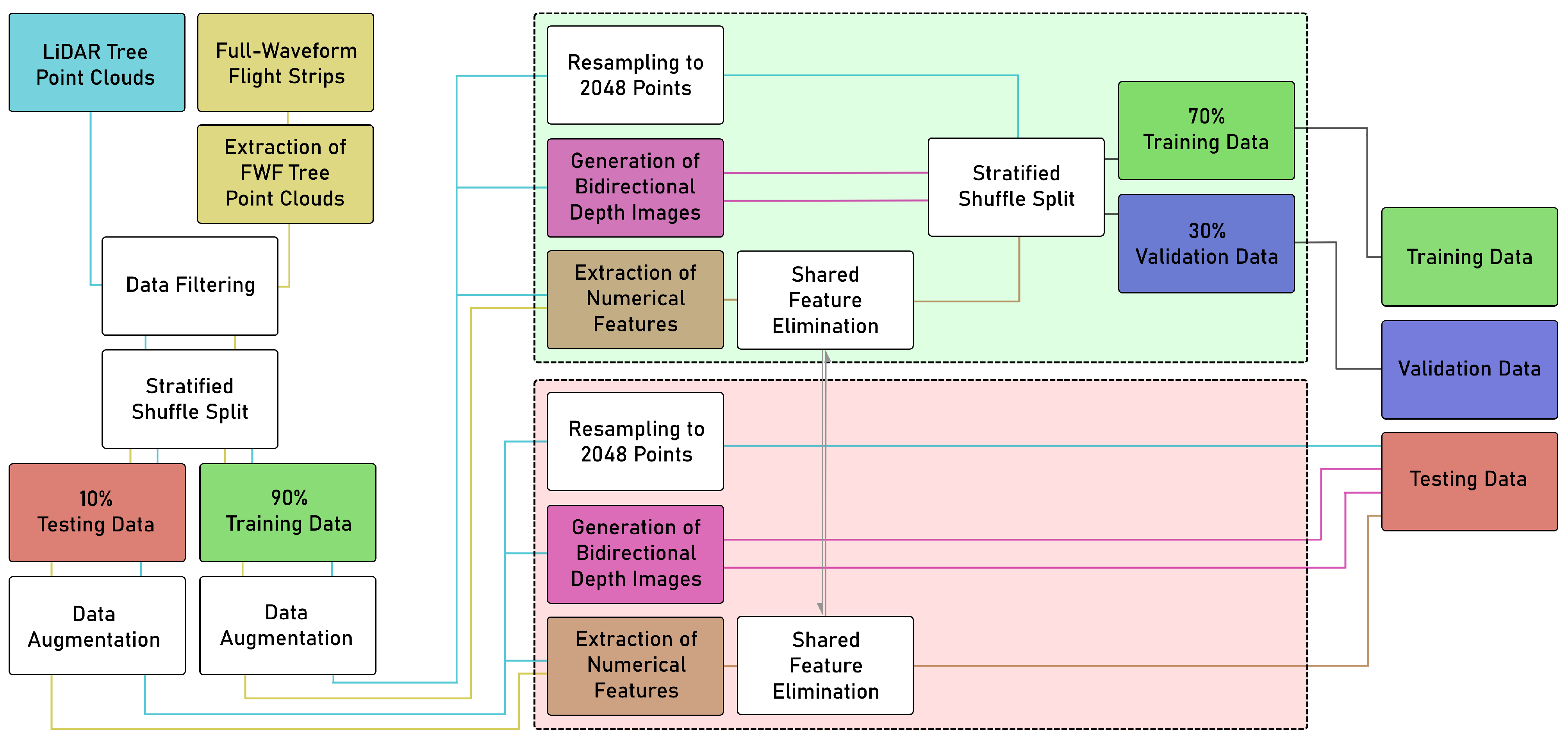
2.2. Data Preprocessing
2.2.1. Point Cloud Augmentation
2.2.2. Generation of Bidirectional Depth Images
2.2.3. Extraction of Numerical Features
2.2.4. Feature Selection
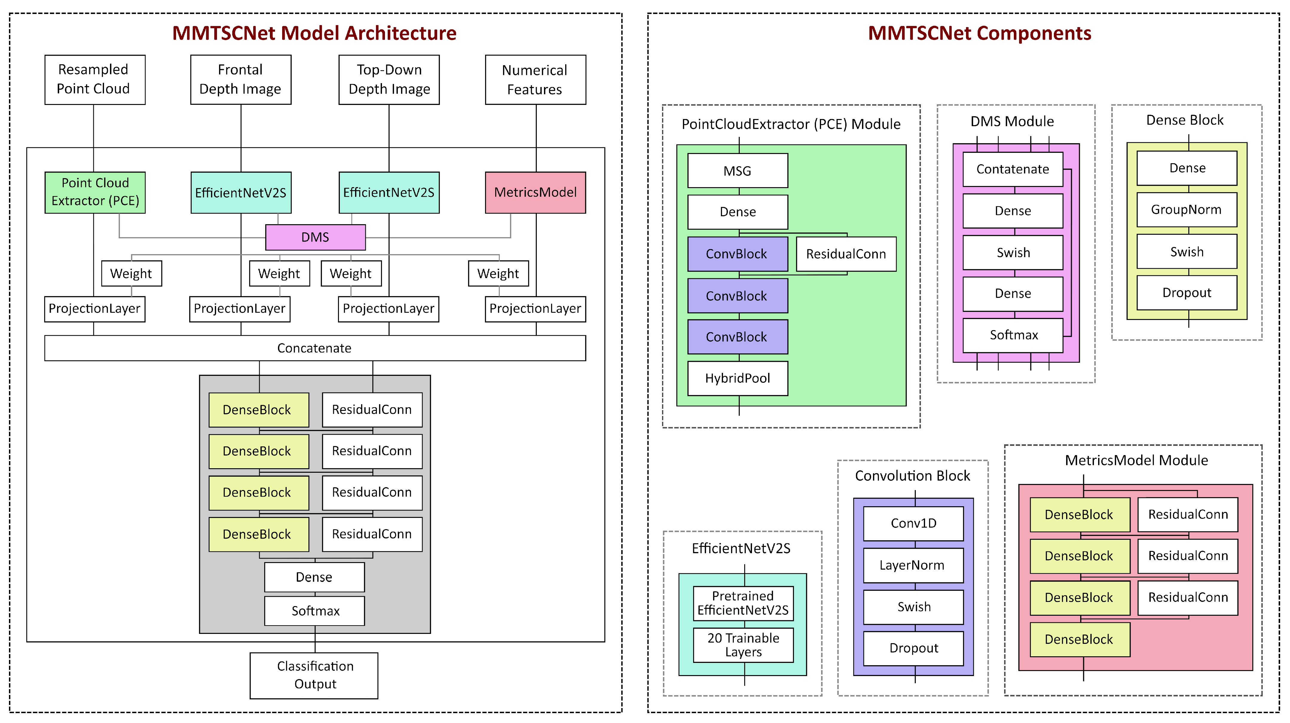
2.3. MMTSCNet Architecture
2.3.1. Point Cloud Extractor Branch
2.3.2. 2D Feature Extraction Branches
2.3.3. Numerical Feature Extraction Branch
2.3.4. Classification Head
2.4. Hyperparameter Tuning and Training
2.5. Other Architectures for Evaluation
2.6. Accuracy Assessment
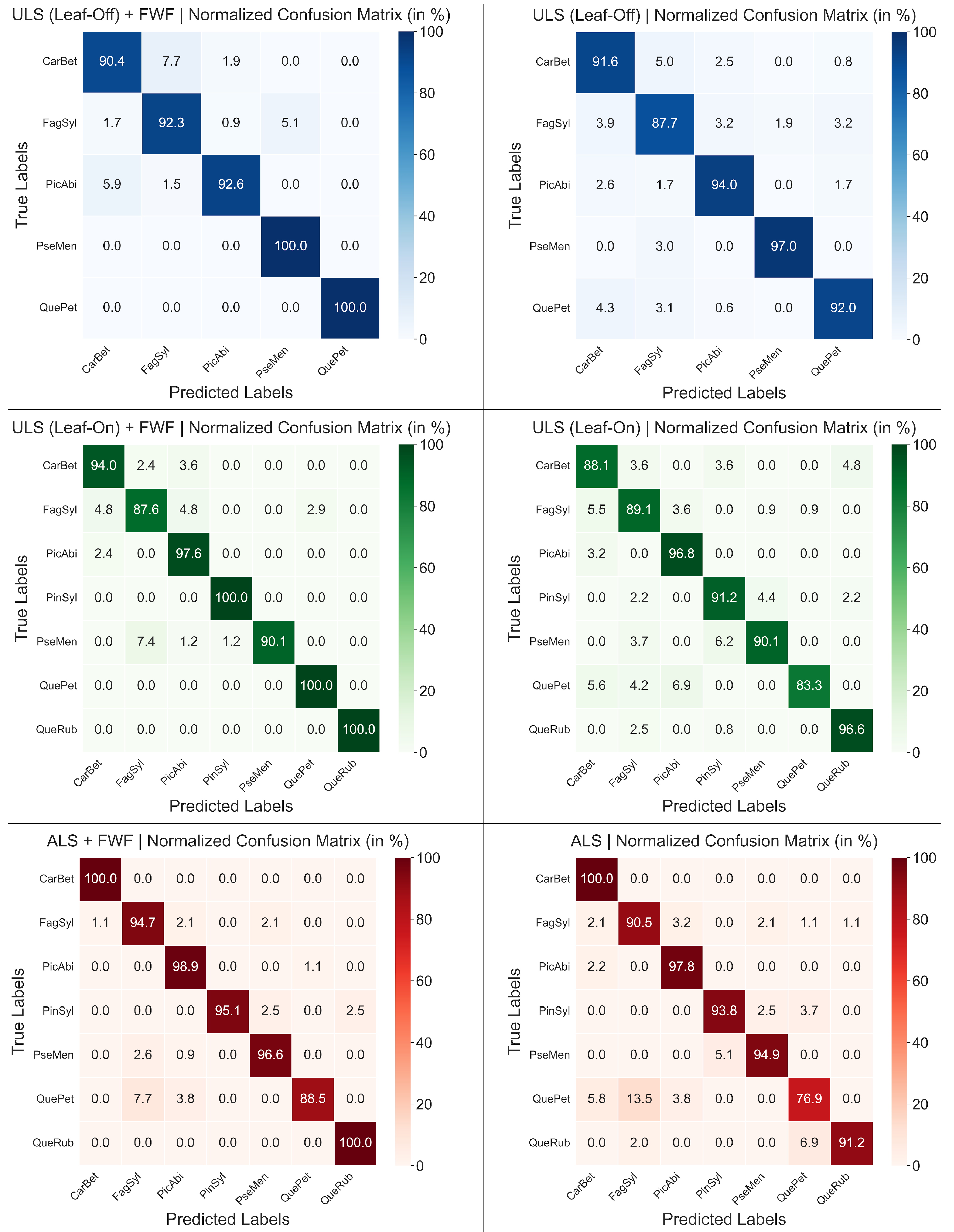
3. Results
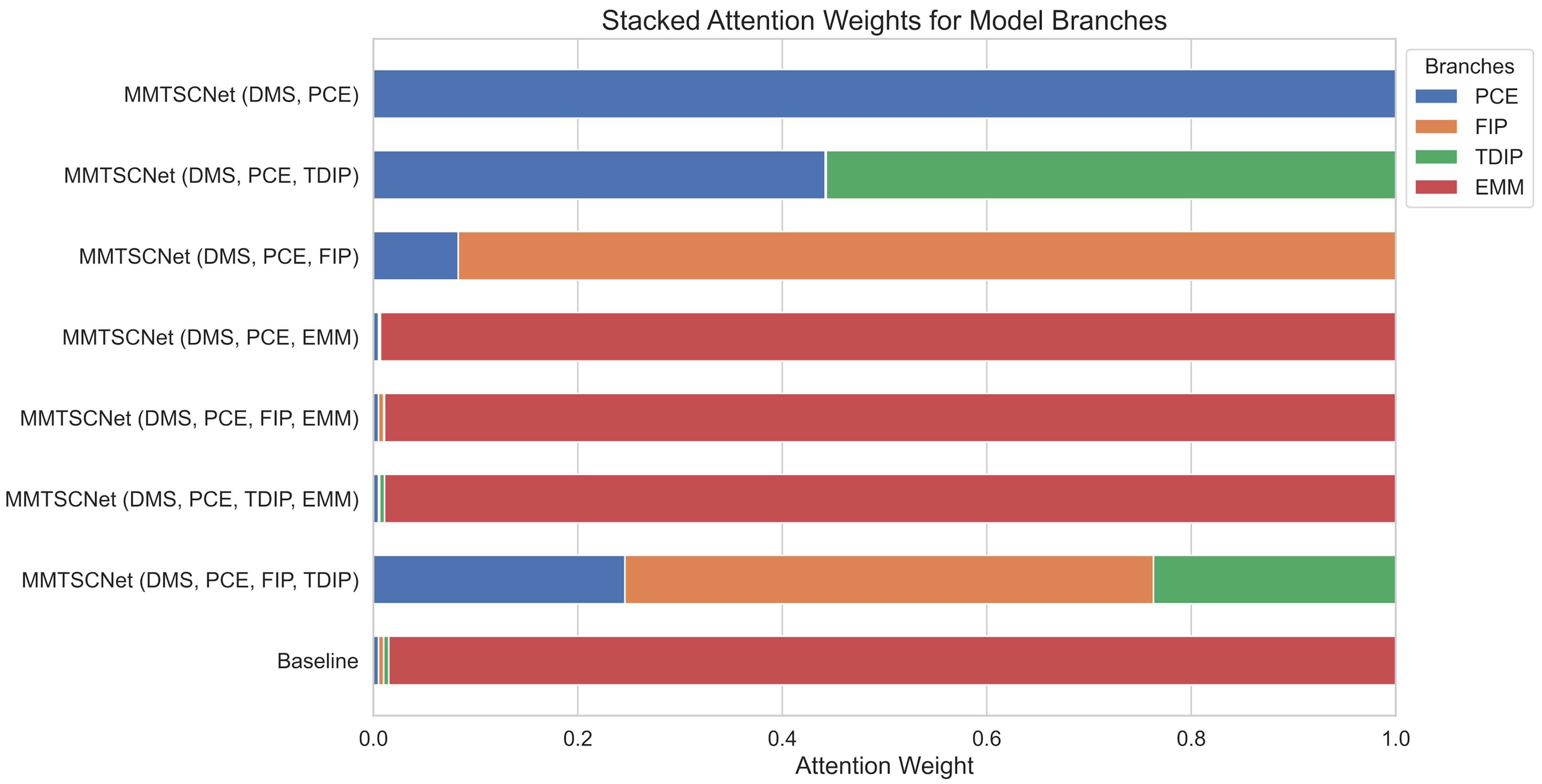
Ablation Study
4. Discussion
4.1. Discussion of Our Results
4.2. Comparison to Other Approaches
5. Conclusions and Outlook
Author Contributions
Funding
Data Availability Statement
Acknowledgments
Conflicts of Interest
References
- Decuyper, M. Combining Conventional Ground-Based and Remotely Sensed Forest Measurements. Ph.D. Thesis, Wageningen University, Wageningen, The Netherlands, 2018. [Google Scholar] [CrossRef]
- Emiliani, G.; Giovannelli, A. Tree Genetics: Molecular and Functional Characterization of Genes. Forests 2023, 14, 534. [Google Scholar] [CrossRef]
- Duncanson, L.; Liang, M.; Leitold, V.; Armston, J.; Krishna Moorthy, S.M.; Dubayah, R.; Costedoat, S.; Enquist, B.J.; Fatoyinbo, L.; Goetz, S.J.; et al. The effectiveness of global protected areas for climate change mitigation. Nat. Commun. 2023, 14, 2908. [Google Scholar] [CrossRef] [PubMed]
- Fettig, C.J.; Klepzig, K.D.; Billings, R.F.; Munson, A.S.; Nebeker, T.E.; Negrón, J.F.; Nowak, J.T. The effectiveness of vegetation management practices for prevention and control of bark beetle infestations in coniferous forests of the western and southern United States. For. Eco. Manag. 2007, 238, 24–53. [Google Scholar] [CrossRef]
- Podgórski, T.; Schmidt, K.; Kowalczyk, R.; Gulczyńska, A. Microhabitat selection by Eurasian lynx and its implications for species conservation. Acta Theriol. 2008, 53, 97–110. [Google Scholar] [CrossRef]
- Kumar, P.; Debele, S.E.; Sahani, J.; Rawat, N.; Marti-Cardona, B.; Alfieri, S.M.; Basu, B.; Basu, A.S.; Bowyer, P.; Charizopoulos, N.; et al. An overview of monitoring methods for assessing the performance of nature-based solutions against natural hazards. Earth-Sci. Rev. 2021, 217, 103603. [Google Scholar] [CrossRef]
- McRoberts, R.; Tomppo, E. Remote sensing support for national forest inventories. Remote Sens. Environ. 2007, 110, 412–419. [Google Scholar] [CrossRef]
- Huete, A.R. Vegetation Indices, Remote Sensing and Forest Monitoring. Geogr. Compass 2012, 6, 513–532. [Google Scholar] [CrossRef]
- Fassnacht, F.E.; Latifi, H.; Stereńczak, K.; Modzelewska, A.; Lefsky, M.; Waser, L.T.; Straub, C.; Ghosh, A. Review of studies on tree species classification from remotely sensed data. Remote Sens. Environ. 2016, 186, 64–87. [Google Scholar] [CrossRef]
- Briechle, S.; Krzystek, P.; Vosselman, G. Classification of tree species and standing dead trees by fusing UAV-based LiDAR data and multispectral imagery in the deep neural network PointNet++. ISPRS Ann. Photogramm. Remote Sens. Spatial Inf. Sci. 2020, V-2-2020, 203–210. [Google Scholar] [CrossRef]
- Hell, M.; Brandmeier, M.; Briechle, S.; Krzystek, P. Classification of Tree Species and Standing Dead Trees with Lidar Point Clouds Using Two Deep Neural Networks: PointCNN and 3DmFV-Net. PFG–J. Photogramm. Remote Sens. Geoinf. Sci. 2022, 90, 103–121. [Google Scholar] [CrossRef]
- Qiao, Y.; Zheng, G.; Du, Z.; Ma, X.; Li, J.; Moskal, L.M. Tree-Species Classification and Individual-Tree-Biomass Model Construction Based on Hyperspectral and LiDAR Data. Remote Sens. 2023, 15, 1341. [Google Scholar] [CrossRef]
- Zhang, Z.; Wang, J.; Wu, Y.; Zhao, Y.; Wu, B. Deeply supervised network for airborne LiDAR tree classification incorporating dual attention mechanisms. GIScience Remote Sens. 2024, 61, 2303866. [Google Scholar] [CrossRef]
- Lin, Y.; Herold, M. Tree species classification based on explicit tree structure feature parameters derived from static terrestrial laser scanning data. Agric. For. Meteorol. 2016, 216, 105–114. [Google Scholar] [CrossRef]
- Fan, Z.; Zhang, W.; Zhang, R.; Wei, J.; Wang, Z.; Ruan, Y. Classification of Tree Species Based on Point Cloud Projection Images with Depth Information. Forests 2023, 14, 2014. [Google Scholar] [CrossRef]
- Lin, Y.; Hyyppä, J. A comprehensive but efficient framework of proposing and validating feature parameters from airborne LiDAR data for tree species classification. Int. J. Appl. Earth Observ. Geoinf. 2016, 46, 45–55. [Google Scholar] [CrossRef]
- Qi, C.R.; Su, H.; Kaichun, M.; Guibas, L.J. PointNet: Deep Learning on Point Sets for 3D Classification and Segmentation. In Proceedings of the 2017 IEEE Conference on Computer Vision and Pattern Recognition, Honolulu, HI, USA, 21–26 July 2017; pp. 77–85. [Google Scholar] [CrossRef]
- Qi, C.R.; Yi, L.; Su, H.; Guibas, L.J. PointNet++: Deep Hierarchical Feature Learning on Point Sets in a Metric Space. In Proceedings of the 31st International Conference on Neural Information Processing Systems, Long Beach, CA, USA, 4–9 December 2017; Volume 31, pp. 5105–5114. [Google Scholar] [CrossRef]
- Tan, M.; Le, Q.V. EfficientNetV2: Smaller Models and Faster Training. In Proceedings of the International Conference on Machine Learning (PMLR), Virtual, 18–24 July 2021; pp. 10096–10106. [Google Scholar] [CrossRef]
- Liu, B.; Chen, S.; Tian, X.; Huang, H.; Ren, M. Tree Species Classification of Point Clouds from Different Laser Sensors Using the PointNet++ Deep Learning Method. In Proceedings of the 2023 IEEE International Geoscience and Remote Sensing Symposium, Pasadena, CA, USA, 16–21 July 2023; pp. 1565–1568. [Google Scholar] [CrossRef]
- Allen, M.J.; Grieve, S.W.D.; Owen, H.J.F.; Lines, E.R. Tree species classification from complex laser scanning data in Mediterranean forests using deep learning. Methods Ecol. Evol. (MEE) 2023, 14, 1657–1667. [Google Scholar] [CrossRef]
- Fan, Z.; Wei, J.; Zhang, R.; Zhang, W. Tree Species Classification Based on PointNet++ and Airborne Laser Survey Point Cloud Data Enhancement. Forests 2023, 14, 1246. [Google Scholar] [CrossRef]
- Chen, J.; Chen, Y.; Liu, Z. Classification of Typical Tree Species in Laser Point Cloud Based on Deep Learning. Remote Sens. 2021, 13, 4750. [Google Scholar] [CrossRef]
- Zhang, C.; Xia, K.; Feng, H.; Yang, Y.; Du, X. Tree species classification using deep learning and RGB optical images obtained by an unmanned aerial vehicle. J. For. Res. 2021, 32, 1879–1888. [Google Scholar] [CrossRef]
- Egli, S.; Höpke, M. CNN-Based Tree Species Classification Using High Resolution RGB Image Data from Automated UAV Observations. Remote Sens. 2020, 12, 3892. [Google Scholar] [CrossRef]
- Schiefer, F.; Kattenborn, T.; Frick, A.; Frey, J.; Schall, P.; Koch, B.; Schmidtlein, S. Mapping forest tree species in high resolution UAV-based RGB-imagery by means of convolutional neural networks. ISPRS J. Photogramm. Remote Sens. 2020, 170, 205–215. [Google Scholar] [CrossRef]
- Reisi Gahrouei, O.; Côté, J.-F.; Bournival, P.; Giguère, P.; Béland, M. Comparison of Deep and Machine Learning Approaches for Quebec Tree Species Classification Using a Combination of Multispectral and LiDAR Data. Can. J. Remote Sens. 2024, 50, 2359433. [Google Scholar] [CrossRef]
- Liu, B.; Hao, Y.; Huang, H.; Chen, S.; Li, Z.; Chen, E.; Tian, X.; Ren, M. TSCMDL: Multimodal Deep Learning Framework for Classifying Tree Species Using Fusion of 2-D and 3-D Features. IEEE Trans. Geosci. Remote Sens. 2023, 61, 4402711. [Google Scholar] [CrossRef]
- Ferreira, M.P.; Dos Santos, D.R.; Ferrari, F.; Filho, L.C.T.C.; Martins, G.B.; Feitosa, R.Q. Improving urban tree species classification by deep-learning based fusion of digital aerial images and LiDAR. Urban For. Urban Green. 2024, 94, 128–240. [Google Scholar] [CrossRef]
- Weiser, H.; Schäfer, J.; Winiwarter, L.; Krašovec, N.; Seitz, C.; Schimka, M.; Anders, K.; Baete, D.; Braz, A.S.; Brand, J.; et al. Terrestrial, UAV-Borne, and Airborne Laser Scanning Point Clouds of Central European Forest Plots, Germany, with Extracted Individual Trees and Manual Forest Inventory Measurements. [Dataset]; PANGAEA: Bremen, Germany, 2022. [Google Scholar] [CrossRef]
- Weiser, H.; Schäfer, J.; Winiwarter, L.; Fassnacht, F.E.; Höfle, B. Airborne Laser Scanning (ALS) Point Clouds with Full-Waveform (FWF) Data of Central European Forest Plots, Germany. [Dataset]; PANGAEA: Bremen, Germany, 2022. [Google Scholar] [CrossRef]
- Felden, J.; Möller, L.; Schindler, U.; Huber, R.; Schumacher, S.; Koppe, R.; Diepenbroek, M.; Glöckner, F.O. PANGAEA—Data Publisher for Earth & Environmental Science. Sci. Data 2023, 10, 347. [Google Scholar] [CrossRef]
- Weiser, H.; Schäfer, J.; Winiwarter, L.; Krašovec, N.; Fassnacht, F.E.; Höfle, B. Individual tree point clouds and tree measurements from multi-platform laser scanning in German forests. Earth Sys. Sci. Data 2022, 14, 2989–3012. [Google Scholar] [CrossRef]
- Deutscher Wetterdienst (DWD). Wetter und Klima—Deutscher Wetterdienst—Presse—Deutschlandwetter im Jahr 2022. 2022. Available online: https://www.dwd.de/DE/presse/pressemitteilungen/DE/2022/20221230_deutschlandwetter_jahr2022_news.html (accessed on 19 January 2025).
- OpenStreetMap Contributors. 2024. Available online: https://download.geofabrik.de (accessed on 19 January 2025).
- Li, J.; Baoxin, H.; Noland, T.L. Classification of tree species based on structural features derived from high-density LiDAR data. Agr. For. Met. 2013, 171/172, 104–114. [Google Scholar] [CrossRef]
- Michałowska, M.; Rapiński, J. A Review of Tree Species Classification Based on Airborne LiDAR Data and Applied Classifiers. Remote Sens. 2021, 13, 353. [Google Scholar] [CrossRef]
- Guo, Y.; Hongsheng, Z.; Qiaosi, L.; Yinyi, L.; Michalski, J. New morphological features for urban tree species identification using LiDAR point clouds. Urban For. Urban Green. 2022, 71, 127558. [Google Scholar] [CrossRef]
- Hovi, A.; Korhonen, L.; Vauhkonen, J.; Korpela, I. LiDAR waveform features for tree species classification and their sensitivity to tree- and acquisition-related parameters. Remote Sens. Environ. 2016, 173, 224–237. [Google Scholar] [CrossRef]
- Shi, Y.; Skidmore, A.K.; Wang, T.; Holzwarth, S.; Heiden, U.; Pinnel, N.; Zhu, X.; Heurich, M. Tree species classification using plant functional traits from LiDAR and hyperspectral data. Int. J. Appl. Earth Obs. Geoinf. 2018, 73, 207–219. [Google Scholar] [CrossRef]
- Shi, Y.; Wang, T.; Skidmore, A.K.; Heurich, M. Important LiDAR metrics for discriminating forest tree species in Central Europe. ISPRS J. Photogramm. Remote Sens. 2018, 137, 163–174. [Google Scholar] [CrossRef]
- Breiman, L. Random Forests. Mach. Learn. 2001, 45, 5–32. [Google Scholar] [CrossRef]
- Deng, J.; Dong, W.; Socher, R.; Li, L.-J.; Li, K.; Fei-Fei, L. ImageNet: A large-scale hierarchical image database. In Proceedings of the 2009 IEEE Conference on Computer Vision and Pattern Recognition, Miami, FL, USA, 20–25 June 2009; pp. 248–255. [Google Scholar] [CrossRef]
- Huang, G.; Liu, Z.; Van Der Maaten, L.; Weinberger, K.Q. Densely Connected Convolutional Networks. In Proceedings of the 2017 IEEE Conference on Computer Vision and Pattern Recognition, Honolulu, HI, USA, 21–26 July 2017; pp. 2261–2269. [Google Scholar] [CrossRef]
- He, K.; Zhang, X.; Ren, S.; Sun, J. Deep Residual Learning for Image Recognition. In Proceedings of the 2016 IEEE Conference on Computer Vision and Pattern Recognition, Las Vegas, NV, USA, 27–30 June 2016; pp. 770–778. [Google Scholar] [CrossRef]
- O’Malley, T.; Bursztein, E.; Long, J.; Chollet, F.; Jin, H.; Invernizzi, L. KerasTuner. GitHub Repository. Version 1.4.7. 2019. Available online: https://keras.io/keras_tuner/ (accessed on 20 January 2025).
- Lin, T.-Y.; Goyal, P.; Girshick, R.; He, K.; Dollár, P. Focal Loss for Dense Object Detection. IEEE Trans. Pattern Anal. Mach. Intell. 2018, 42, 318–327. [Google Scholar] [CrossRef]
- Puliti, S.; Lines, E.; Müllerová, J.; Frey, J.; Schindler, Z.; Straker, A.; Allen, M.; Winiwarter, L.; Rehush, N.; Hristova, H.; et al. Benchmarking tree species classification from proximally-sensed laser scanning data: Introducing the FOR-species20K dataset. Methods Ecol. Evol. (MEE) 2025, 16, 801–818. [Google Scholar] [CrossRef]


| Species (Latin) | Mean Height | Height STD | Mean Point Density per m3 (ALS) | Mean Point Density per m3 (ULS) | Samples (ALS) | Samples (ULS Leaf-On) | Samples (ULS Leaf-Off) | Leaf Morph. |
|---|---|---|---|---|---|---|---|---|
| Abies alba | 23.70 | 6.89 | 2.76 | 35.02 | 20 | 7 | 12 | Coniferous |
| Acer campestre | 12.34 | 7.16 | 3.93 | 27.21 | 7 | 6 | 11 | Broad-Leaved |
| Acer pseudoplantanus | 19.17 | 7.77 | 2.87 | 19.41 | 39 | 36 | 39 | Broad-Leaved |
| Betula pendula | 20.16 | 6.14 | 4.35 | 29.95 | 6 | 4 | 4 | Broad-Leaved |
| Carpinus betulus | 15.68 | 5.44 | 2.27 | 15.36 | 90 | 89 | 132 | Broad-Leaved |
| Fagus sylvatica | 23.42 | 7.74 | 2.62 | 19.27 | 397 | 366 | 509 | Broad-Leaved |
| Fraxinus excelsior | 14.47 | 6.04 | 3.21 | 21.60 | 11 | 10 | 18 | Broad-Leaved |
| Juglans regia | 16.80 | 3.91 | 2.74 | 12.04 | 19 | 19 | 19 | Broad-Leaved |
| Larix decidua | 33.77 | 4.00 | 2.36 | 26.05 | 30 | 30 | 36 | Coniferous |
| Picea abies | 18.81 | 5.98 | 4.21 | 30.09 | 205 | 200 | 331 | Coniferous |
| Pinus sylvestris | 29.95 | 3.47 | 2.33 | 25.52 | 158 | 103 | 79 | Coniferous |
| Prunus avium | 16.14 | 3.71 | 3.28 | 18.61 | 19 | 19 | 37 | Broad-Leaved |
| Prunus serotina | 11.11 | 2.49 | 3.94 | 0.00 | 7 | 0 | 0 | Broad-Leaved |
| Pseudotsuga menziesii | 36.84 | 5.51 | 2.03 | 22.11 | 191 | 140 | 164 | Coniferous |
| Quercus petraea | 18.88 | 7.48 | 3.82 | 25.45 | 156 | 152 | 262 | Broad-Leaved |
| Quercus robur | 27.87 | 2.58 | 3.07 | 25.26 | 7 | 6 | 6 | Broad-Leaved |
| Quercus rubra | 22.47 | 4.03 | 3.09 | 44.23 | 111 | 92 | 9 | Broad-Leaved |
| Robinia pseudoacacia | 11.34 | 0.00 | 4.42 | 0.00 | 1 | 0 | 0 | Broad-Leaved |
| Salix caprea | 16.79 | 0.14 | 4.36 | 21.94 | 1 | 1 | 2 | Broad-Leaved |
| Sorbus torminalis | 13.55 | 0.21 | 0.00 | 5.32 | 0 | 1 | 1 | Broad-Leaved |
| Tilia (Not Specified) | 21.12 | 3.49 | 2.18 | 18.82 | 4 | 4 | 4 | Broad-Leaved |
| Tsuga heterophylla | 19.91 | 0.07 | 1.36 | 12.97 | 1 | 1 | 1 | Coniferous |
| Plot | ALS (Leaf-On) | ULS (Leaf-On) | ULS (Leaf-Off) |
|---|---|---|---|
| BR01 | 514 | 503 | 503 |
| BR02 | 42 | 42 | 41 |
| BR03 | 195 | 141 | 141 |
| BR04 | 9 | - | - |
| BR05 | 278 | 278 | 278 |
| BR06 | 29 | 29 | 29 |
| BR07 | 15 | 16 | 15 |
| BR08 | 13 | 13 | 12 |
| KA09 | 177 | 136 | 133 |
| KA10 | 30 | 14 | - |
| KA11 | 151 | 97 | - |
| SP02 | 17 | 17 | 21 |
| All plots | 1480 | 1286 | 1173 |
| Dataset | ALS + FWF | ULS (Leaf-On) + FWF | ULS (Leaf-Off) + FWF | ALS | ULS (Leaf-On) | ULS (Leaf-Off) |
|---|---|---|---|---|---|---|
| FagSyl | 790 | 860 | 1167 | 790 | 880 | 1245 |
| CarBet | 667 | 735 | 630 | 667 | 840 | 1088 |
| PicAbi | 720 | 1035 | 1657 | 720 | 1035 | 1926 |
| PinSyl | 684 | 754 | x | 684 | 754 | x |
| PseMen | 1008 | 720 | 1328 | 1008 | 720 | 1365 |
| QuePet | 494 | 603 | 969 | 494 | 612 | 1350 |
| QueRub | 936 | 1088 | x | 936 | 1088 | x |
| Name | Symbol | Derived From |
|---|---|---|
| Intensity Kurtosis | FWF | |
| Mean Pulse Width | FWF | |
| Intensity Mean | FWF | |
| Intensity Standard Deviation | FWF | |
| Intensity Contrast | FWF | |
| Echo Width | W | FWF |
| FHWM | FWF |
| Name | Symbol | Derived From |
|---|---|---|
| Point Density | ALS/ULS | |
| Leaf Area Index | ALS/ULS | |
| Crown Shape Indices | ALS/ULS | |
| Point Density for Normalized Height Bin j | ALS/ULS | |
| Relative Clustering Degree | ALS/ULS | |
| Average Nearest Neighbor Distance | ALS/ULS | |
| Canopy Closure | ALS/ULS | |
| Entropy of Height Distribution | ALS/ULS | |
| Crown Volume | ALS/ULS | |
| Canopy Surface-to-Volume Ratio | ALS/ULS | |
| Equivalent Crown Diameter | ALS/ULS | |
| Fractal Dimension (k = 2) | ALS/ULS | |
| Main Component (PCA) Eigenvalues | , | ALS/ULS |
| Linearity | ALS/ULS | |
| Sphericity | ALS/ULS | |
| Planarity | ALS/ULS | |
| Maximum Crown Diameter | ALS/ULS | |
| Height Kurtosis | ALS/ULS | |
| Height Skewness | ALS/ULS | |
| Height Standard Deviation | ALS/ULS | |
| Leaf Inclination | ALS/ULS | |
| Convex Hull Compactness | ALS/ULS | |
| Crown Asymmetry | ALS/ULS | |
| Leaf Curvature | ALS/ULS | |
| N-th Percentile of Height Distribution | ALS/ULS | |
| Canopy Cover Fraction | ALS/ULS | |
| Canopy Ellipticity | ALS/ULS | |
| Gini Coefficient for Height Distribution | ALS/ULS | |
| Branch Density | ALS/ULS | |
| Height Variation Coefficient | ALS/ULS | |
| Crown Symmetry | ALS/ULS | |
| Crown Curvature | ALS/ULS | |
| Canopy Width x and y | ALS/ULS | |
| Density Gradient | ALS/ULS | |
| Surface Roughness | ALS/ULS | |
| Segment Density for Height Bin i | ALS/ULS |
| Hyperparameter | Selected Value |
|---|---|
| PCE Depth | 3 |
| PCE Convolution Filters | 256 |
| PCE Number of NN | 24 |
| PCE MSG Radii | 0.055, 0.135, 0.345, 0.525, 0.695 |
| EMM Dense Units | 512 |
| Classification Head Projection Units | 128 |
| Classification Head Depth | 4 |
| Classification Dense Units | 512 |
| Metric Name | Formula |
|---|---|
| MAP (Macro Average Precision) | |
| MAR (Macro Average Recall) | |
| MAF (Macro Average F1-Score) | |
| OA (Overall Accuracy) | |
| Cohens’ Kappa Score |
| Dataset | OA | MAF | MAP | MAR | Kappa Coefficient | Species |
|---|---|---|---|---|---|---|
| ALS | 0.928 | 0.923 | 0.929 | 0.928 | 0.915 | 7 |
| ALS + FWF | 0.966 | 0.966 | 0.967 | 0.966 | 0.960 | 7 |
| ULS Leaf-On | 0.915 | 0.915 | 0.917 | 0.915 | 0.900 | 7 |
| ULS Leaf-On + FWF | 0.957 | 0.958 | 0.957 | 0.957 | 0.949 | 7 |
| ULS Leaf-Off | 0.927 | 0.928 | 0.929 | 0.927 | 0.908 | 5 |
| ULS Leaf-Off + FWF | 0.954 | 0.952 | 0.956 | 0.955 | 0.941 | 5 |
| Data Subset | Metric | CarBet | FagSyl | PicAbi | PinSyl | PseMen | QuePet | QueRub |
|---|---|---|---|---|---|---|---|---|
| ALS | F1-Score | 0.94 | 0.91 | 0.96 | 0.93 | 0.96 | 0.78 | 0.95 |
| Precision | 0.89 | 0.91 | 0.95 | 0.93 | 0.97 | 0.78 | 0.99 | |
| Recall | 1.00 | 0.91 | 0.98 | 0.94 | 0.95 | 0.77 | 0.91 | |
| ALS + FWF | F1-Score | 0.99 | 0.94 | 0.97 | 0.97 | 0.97 | 0.93 | 0.99 |
| Precision | 0.98 | 0.93 | 0.95 | 1.0 | 0.97 | 0.98 | 0.98 | |
| Recall | 1.00 | 0.95 | 0.99 | 0.95 | 0.97 | 0.89 | 1.00 | |
| ULS Leaf-On | F1-Score | 0.88 | 0.87 | 0.95 | x | 0.98 | 0.93 | x |
| Precision | 0.85 | 0.87 | 0.96 | x | 0.98 | 0.94 | x | |
| Recall | 0.92 | 0.88 | 0.94 | x | 0.97 | 0.92 | x | |
| ULS Leaf-Off + FWF | F1-Score | 0.86 | 0.96 | 0.95 | x | 0.98 | 1.00 | x |
| Precision | 0.82 | 0.95 | 0.98 | x | 0.96 | 1.00 | x | |
| Recall | 0.90 | 0.92 | 0.93 | x | 1.00 | 1.00 | x | |
| ULS Leaf-On | F1-Score | 0.86 | 0.88 | 0.95 | 0.91 | 0.92 | 0.90 | 0.96 |
| Precision | 0.84 | 0.88 | 0.93 | 0.90 | 0.94 | 0.98 | 0.95 | |
| Recall | 0.88 | 0.89 | 0.97 | 0.91 | 0.90 | 0.83 | 0.97 | |
| ULS Leaf-On + FWF | F1-Score | 0.92 | 0.90 | 0.95 | 0.99 | 0.95 | 0.98 | 1.00 |
| Precision | 0.91 | 0.92 | 0.93 | 0.99 | 1.00 | 0.96 | 1.00 | |
| Recall | 0.94 | 0.88 | 0.98 | 1.00 | 0.90 | 1.00 | 1.00 |
| Data Subset | Model | OA | MAF | MAP | MAR | Kappa Coefficient | Species |
|---|---|---|---|---|---|---|---|
| ALS | PointNet++ (FPS) | 0.83 | 0.82 | 0.83 | 0.82 | 0.80 | 7 |
| ALS | PointNet++ (RS) | 0.83 | 0.83 | 0.83 | 0.83 | 0.80 | 7 |
| ALS | PointNet++ (GAS) | 0.85 | 0.84 | 0.85 | 0.84 | 0.82 | 7 |
| ALS | PointNet++ (NGS) | 0.85 | 0.85 | 0.86 | 0.85 | 0.83 | 7 |
| ALS | PointNet++ (KS) | 0.86 | 0.86 | 0.87 | 0.86 | 0.84 | 7 |
| ALS | DSTCN | 0.94 | 0.94 | 0.95 | 0.95 | 0.93 | 7 |
| ALS | MMTSCNet | 0.93 | 0.92 | 0.93 | 0.93 | 0.91 | 7 |
| ALS + FWF | MMTSCNet | 0.97 | 0.97 | 0.97 | 0.97 | 0.96 | 7 |
| ULS Leaf-On | PointNet++ (NGFPS) | 0.90 | x | x | x | 0.86 | 4 |
| ULS Leaf-On | MMTSCNet | 0.92 | 0.92 | 0.92 | 0.92 | 0.90 | 7 |
| ULS Leaf-On + FWF | MMTSCNet | 0.96 | 0.96 | 0.96 | 0.96 | 0.95 | 7 |
| ULS Leaf-Off | PointNet++ (NGFPS) | 0.89 | x | x | x | 0.84 | 4 |
| ULS Leaf-Off | MMTSCNet | 0.93 | 0.93 | 0.93 | 0.93 | 0.90 | 5 |
| ULS Leaf-Off + FWF | MMTSCNet | 0.95 | 0.95 | 0.96 | 0.96 | 0.94 | 5 |
| Active Modules | Disabled Modules | OA | MAF | MAP | MAR | Kappa Coefficient |
|---|---|---|---|---|---|---|
| DMS, PCE, FIP, TDIP, EMM | x | 0.97 | 0.97 | 0.97 | 0.97 | 0.96 |
| DMS, PCE, FIP, TDIP | EMM | 0.84 | 0.79 | 0.81 | 0.81 | 0.75 |
| DMS, PCE, FIP, EMM | TDIP | 0.88 | 0.88 | 0.89 | 0.88 | 0.73 |
| DMS, PCE, TDIP, EMM | FIP | 0.90 | 0.89 | 0.90 | 0.89 | 0.80 |
| DMS, PCE, EMM | FIP, TDIP | 0.90 | 0.89 | 0.90 | 0.89 | 0.74 |
| DMS, PCE, FIP | TDIP, EMM | 0.86 | 0.83 | 0.83 | 0.84 | 0.90 |
| DMS, PCE, TDIP | FIP, EMM | 0.63 | 0.58 | 0.62 | 0.62 | 0.22 |
| DMS, PCE | FIP, TDIP, EMM | 0.48 | 0.45 | 0.58 | 0.48 | 0.08 |
| PCE, FIP, TDIP, EMM | DMS | 0.82 | 0.83 | 0.86 | 0.83 | 0.61 |
Disclaimer/Publisher’s Note: The statements, opinions and data contained in all publications are solely those of the individual author(s) and contributor(s) and not of MDPI and/or the editor(s). MDPI and/or the editor(s) disclaim responsibility for any injury to people or property resulting from any ideas, methods, instructions or products referred to in the content. |
© 2025 by the authors. Licensee MDPI, Basel, Switzerland. This article is an open access article distributed under the terms and conditions of the Creative Commons Attribution (CC BY) license (https://creativecommons.org/licenses/by/4.0/).
Share and Cite
Vahrenhold, J.R.; Brandmeier, M.; Müller, M.S. MMTSCNet: Multimodal Tree Species Classification Network for Classification of Multi-Source, Single-Tree LiDAR Point Clouds. Remote Sens. 2025, 17, 1304. https://doi.org/10.3390/rs17071304
Vahrenhold JR, Brandmeier M, Müller MS. MMTSCNet: Multimodal Tree Species Classification Network for Classification of Multi-Source, Single-Tree LiDAR Point Clouds. Remote Sensing. 2025; 17(7):1304. https://doi.org/10.3390/rs17071304
Chicago/Turabian StyleVahrenhold, Jan Richard, Melanie Brandmeier, and Markus Sebastian Müller. 2025. "MMTSCNet: Multimodal Tree Species Classification Network for Classification of Multi-Source, Single-Tree LiDAR Point Clouds" Remote Sensing 17, no. 7: 1304. https://doi.org/10.3390/rs17071304
APA StyleVahrenhold, J. R., Brandmeier, M., & Müller, M. S. (2025). MMTSCNet: Multimodal Tree Species Classification Network for Classification of Multi-Source, Single-Tree LiDAR Point Clouds. Remote Sensing, 17(7), 1304. https://doi.org/10.3390/rs17071304