Estimating Chlorophyll-a Concentrations in Optically Shallow Waters Using Gaofen-1 Wide-Field-of-View (GF-1 WFV) Datasets from Lake Taihu, China

Abstract

Lake Taihu has highly turbid inland waters with complex optical properties. Due to the bottom effect of submerged aquatic plants in optically shallow waters, currently available phytoplankton chlorophyll-a retrieval algorithms tend to overestimate chlorophyll-a concentrations in the eastern part of Lake Taihu. This overestimation can distort the eutrophication evaluation of the entire lake. This paper identifies submerged and emergent plants, determines the retrieval models for the upwelling (K_u) and downwelling (K_d) irradiance attenuation coefficients, and proposes a phytoplankton chlorophyll-a retrieval model using a water depth optimization-based method to remove the bottom effect. The results show the following: (1) The normalized difference vegetation index (NDVI) method can distinguish the bottom mud (NDVI < −0.46) and submerged aquatic plants (−0.46 ≤ NDVI < 0.52) from the emergent plants (NDVI ≥ 0.52) with 90% accuracy. (2) The downwelling and upwelling irradiance attenuation coefficients are highly correlated with the suspended sediments, and retrieval models for these coefficients in three visible bands with high accuracy are presented. (3) Compared to traditional algorithms without bottom effect removal, the proposed chlorophyll-a concentration estimation algorithm based on the water depth-optimized bottom effect removal method efficiently reduces the bottom effect of the submerged aquatic plants. The root mean square error (RMSE) for the obtained chlorophyll-a concentrations decreases from 45.61 ${\mathsf{\mu }\mathrm{g}·\mathrm{L}}^{-1}$ to 8.69 ${\mathsf{\mu }\mathrm{g}·\mathrm{L}}^{-1}$, and the mean absolute percentage error (MAPE) is reduced from 245.12% to 19.58%. In the validation step, the obtained RMSE of 10.89 ${\mathsf{\mu }\mathrm{g}·\mathrm{L}}^{-1}$ and MAPE of 17.52% are consistent with the proposed algorithm. This research provides a good reference for the determination of chlorophyll-a concentrations in phytoplankton in complex inland water bodies. The findings are potentially useful for the operational monitoring of harmful algal blooms in the future.

1. Introduction

Optical radiative transfer in optically shallow water refers to the process where the sunlight penetrates the air–water interface, reaches the bottom, and then is scattered back to the satellite sensor. The incident spectrum is altered by the absorption and scattering of optically active substances and the selective reflection by the bottom [1]. During this process, satellite sensors acquire the spectral features of optically active substances, such as chlorophyll-a, suspended sediments, and chromophoric dissolved organic matter (CDOM), also referred to as gelbstoff, gilvin, or yellow substance, in water bodies and the underwater bottom substrate [2]. For optically deep waters, the bottom effect can be ignored. However, for optically shallow waters, the contribution of the submerged aquatic plants to the water-leaving radiance is quite significant and varies with the bottom depth (H), the inherent optical properties (IOPs) of the water column, and the bottom albedo ρ(λ) [3,4,5].

Currently, the majority of remote sensing inversion algorithms for chlorophyll-a in marine phytoplankton are mainly designed for optically deep waters, ignoring the bottom effect. In case 1 waters, ocean chlorophyll-x (OC-x) algorithms based on blue–green bands are often employed [6,7,8]. In case 2 waters, a red-shift phenomenon occurs in the blue–green algorithm, as seen in the ratio of the remote sensing reflectance at wavelengths of 488 nm (blue band) and 551 nm (green band)—Rs(488)/Rs(551) [9,10]. In inland waters, the absorption peak of phytoplankton in the 440 nm band is often overshadowed by suspended sediments and colored dissolved organic matter with stronger absorption. As a result, empirical algorithms typically use red-edge or red ratio algorithms [11,12,13,14], neural network methods [15,16,17], and three-band methods [18,19,20]. These algorithms are not only used for optically deep waters; they are actually universally applied to all waters [21,22], and their performance is reduced by the bottom effect when applied to optically shallow waters. Alternatively, semi-analytical or analytical algorithms can simplify the radiative transfer equations and provide estimates of geophysical properties [23]. The apparent optical properties (AOPs) of water bodies can be expressed as a function of IOPs, H, and the bottom ρ(λ) using analytical model methods [24] in optically shallow waters. Numerous inversion techniques for determining chlorophyll-a concentrations in phytoplankton in optically shallow water [25,26,27,28,29] have been developed based on analytical models. Among them, the water depth (${\mathrm{Z}}_{\mathrm{B}}$) and the ρ(λ) of the bottom surface (with a thickness or height of approximately 0) directly affect the inversion accuracy of chlorophyll-a concentrations. Field experimental data show that the height (h) of submerged aquatic plants superimposed on specific terrain with varying water depths (${\mathrm{Z}}_{\mathrm{B}}$) can vary greatly. The closer the top of submerged aquatic plants to the water surface, the greater the contribution of aquatic plants to the reflectance spectra [30,31]. Given ρ(λ) and ${\mathrm{Z}}_{\mathrm{B}}$, the different (h) values of submerged aquatic plants have a significant influence on the remote sensing reflectance. Thus, it is not ${\mathrm{Z}}_{\mathrm{B}}$ but rather the equivalent ${\mathrm{Z}}_{\mathrm{B}}^{\prime }$ (${\mathrm{Z}}_{\mathrm{B}}^{\prime }$ = ${\mathrm{Z}}_{\mathrm{B}}$ − h) that affects the contribution of the submerged aquatic plants to the water-leaving signals.

Lake Taihu is the third-largest freshwater lake in China, covering an area of approximately 2427.8 square kilometers, with an average water depth of 1.9 m and a maximum water depth of 2.6 m. It has typical highly turbid inland waters with complex optical properties. In addition to the optically deep areas with high turbidity in the western part of Lake Taihu, there are also typical optically shallow areas, such as those noted in the eastern part of Lake Taihu, where the water is clear, and the underwater vegetation is lush. The spectral reflectance of submerged aquatic plants with different h values superimposed on specific terrain with varying ${\mathrm{Z}}_{\mathrm{B}}\mathrm{v}\mathrm{a}\mathrm{l}\mathrm{u}\mathrm{e}\mathrm{s}$ can vary greatly. The closer the top of a submerged aquatic plant is to the water surface, the greater the bottom effect of the aquatic plant. The different h values of submerged aquatic plants significantly influence the water-leaving radiance, and the chlorophyll-a concentration in phytoplankton is inevitably overestimated in optically shallow waters. This overestimation would prevent an accurate evaluation of the eutrophication level of water bodies [15,16,32,33,34,35]. Many researchers have rigidly masked out the optically shallow waters in the eastern part of Lake Taihu. These researchers do not monitor the water quality and its changes in the eastern part of Taihu Lake, which accounts for nearly one-third of the entire Lake Taihu [12,36,37,38]. This poses a significant limitation when monitoring the entire Lake Taihu. Therefore, it is necessary to consider the different h values of submerged aquatic plants, as well as the actual ${\mathrm{Z}}_{\mathrm{B}}$, and develop a bottom effect removal method based on water depth optimization ${\mathrm{Z}}_{\mathrm{B}}^{\prime }$ to reduce retrieval errors of phytoplankton chlorophyll-a concentrations in the optically shallow waters of Taihu Lake.

In this study, which used cruise data collected in 2003, 2007, 2009, and 2024, combined with Gaofen-1 Wide-Field-of-View (GF-1 WFV) data from 2024, a normalized difference vegetation index (NDVI)-based method for identifying submerged aquatic plants from emergent vegetation is proposed, and remote sensing-based retrieval models for downwelling and upwelling irradiance attenuation coefficients in the red, green, and blue bands of the GF-1 WFV datasets in Lake Taihu are proposed. Moreover, a water depth optimization-based bottom effect removal method is proposed that can effectively reduce the retrieval errors of phytoplankton chlorophyll-a concentrations in optically shallow waters.

2. Datasets and Methods

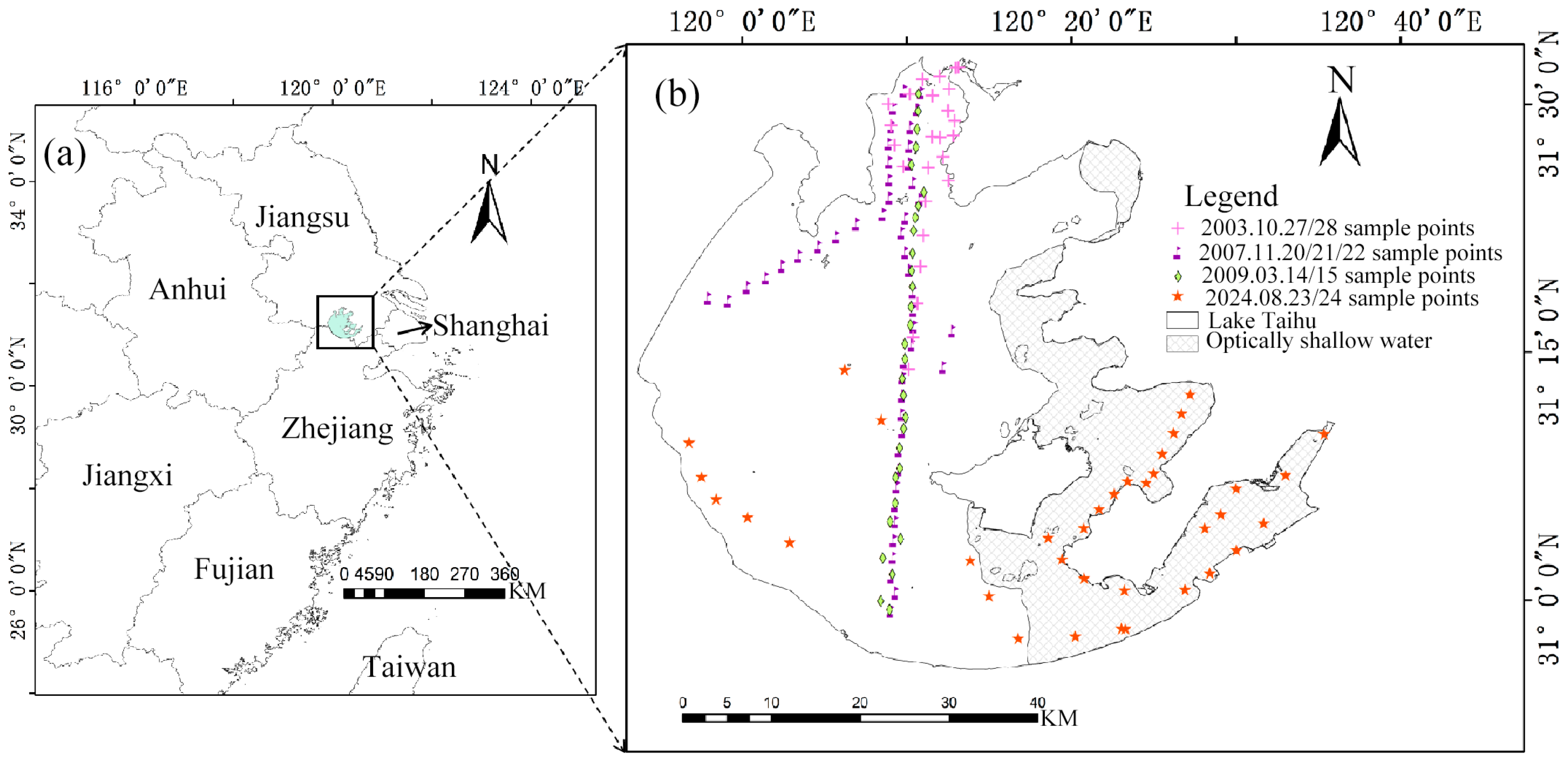
2.1. Datasets

This study adopted data from four cruises that are synchronous with satellite overpasses, i.e., the pre-research project of the HJ satellite (HJ-2003) in 2003, the Knowledge Innovation Project of the Chinese Academy of Sciences (KI-2007) in 2007, the Major Interdisciplinary Project of the Chinese Academy of Sciences (MIPCAS-2009) in 2009, and the National Key Research and Development Project (NKRD-2024) in 2024. The dataset includes 118 samples from optically deep waters (25 samples from the HJ-2003 cruise, 50 samples from the KI-2007 cruise, 33 samples from the MIPCAS-2009 cruise, and 10 samples from the NKRD-2024 cruise) and 36 samples from optically shallow waters (9 samples from bottom mud, 19 samples from submerged aquatic plants, and 8 survey samples from emergent plants in the NKRD-2024 cruise dataset). The field measurement locations in Lake Taihu are shown in Figure 1. The basic information of the synchronous experiments is summarized in

Table 1. Summary of the data from four cruises conducted synchronously with satellite overpasses in Lake Taihu.

Cruise	Location	Dates	Chlorophyll-a (μg · L−1)
			Mean	Standard Deviation	Minimum	Maximum
HJ-2003	Meiliang Bay	27–28 October 2003	42.16	56.47	2.20	230.59
KI-2007	Meiliang Bay–West Lake Taihu	20–22 November 2007	44.90	74.83	7.25	387.11
MIPCAS-2009	Meiliang Bay–Huzhou County	14–15 March 2009	10.41	16.51	5.41	54.07
NKRD-2024	Eastern–Southwest Lake Taihu	23–24 August 2024	62.77	123.88	2.00	495.00

.

2.1.1. Water Quality Parameters

Water samples were collected in the upper 5–20 cm of the water column using a pre-rinsed 2 L bottle and kept in the dark at a temperature of 4 °C in a refrigerator. The water samples were filtered using a GF/C filter membrane, and the membrane was placed in the refrigerator for at least 48 h. Chlorophyll-a was extracted in 90% hot ethanol, and the absorbance at 665 and 750 nm with dilute hydrochloric acid acidification at a temperature of 80–85° was determined with a SHIMADZU UV-2401 spectrophotometer (manufactured by Shimadzu Corporation, Kyoto, Japan). The concentrations of total suspended sediments (TSS) were measured gravimetrically [39].

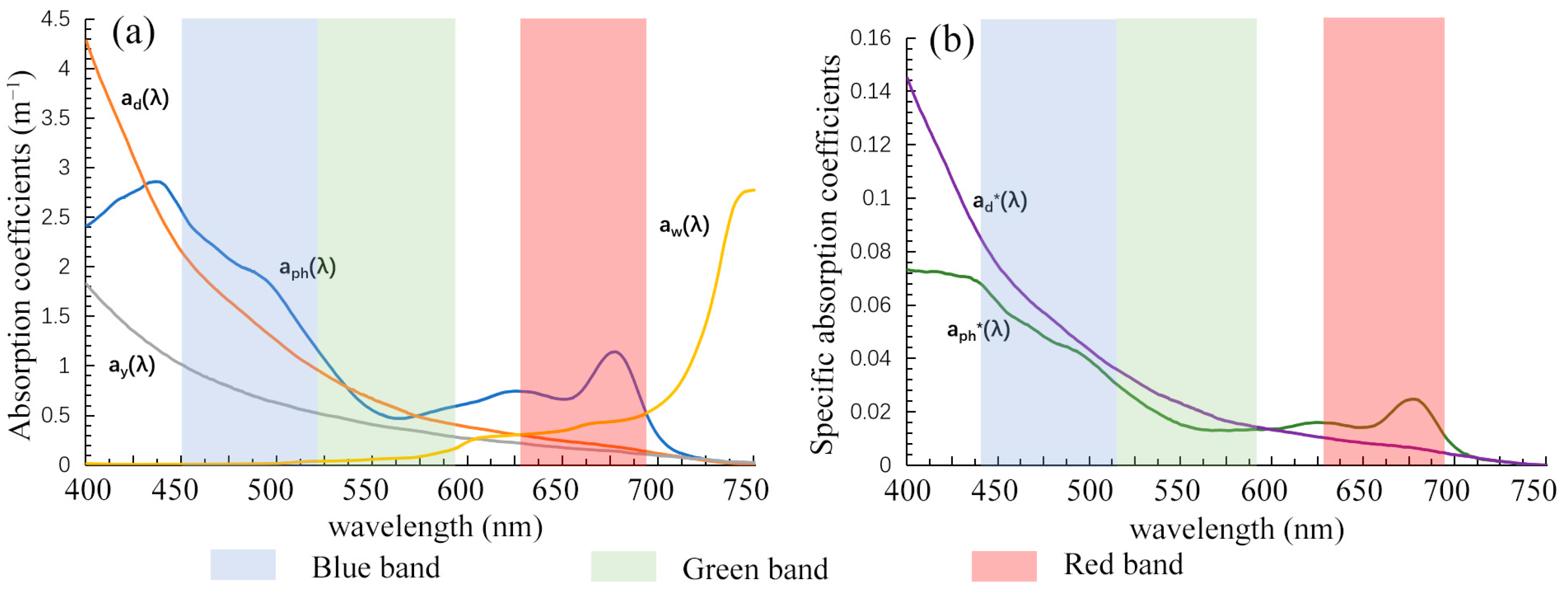
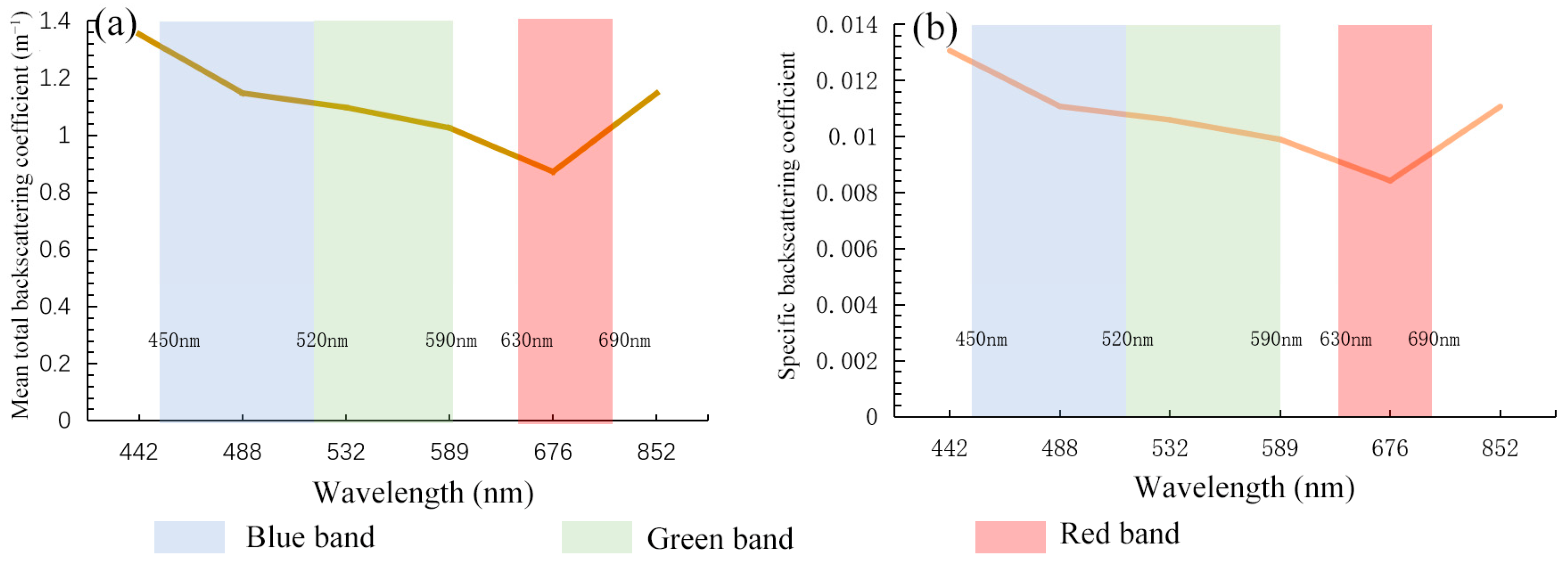
2.1.2. Measurements of IOPs

(1)

Absorption Coefficients

The SHIMADZU UV-2401 spectrophotometer was used in the laboratory to measure the inherent optical properties of water components, including the absorption coefficients of yellow substances, ${\mathrm{a}}_{\mathrm{y}}(\mathsf{\lambda })$; the absorption coefficients of total suspended particulate matter, ${\mathrm{a}}_{\mathrm{p}}(\mathsf{\lambda })$; and the absorption coefficients of algal particulate matter, ${\mathrm{a}}_{\mathrm{p}\mathrm{h}}(\mathsf{\lambda })$. All the measurements were performed according to the National Aeronautics and Space Administration (NASA) Ocean Optics Protocols [40].

(2)

Backscattering Coefficients

The backscattering coefficients were measured using a HydroScat-6 Spectral Backscattering Sensor (HS-6, HOBI Lab, Inc., Tucson, AZ, USA) at 442, 488, 532, 589, 676, and 852 nm wavelengths. The instrument was calibrated, and the field measurements were performed with a sigma correction.

2.1.3. AOP Measurements

(1)

Underwater Irradiance Measurements

Underwater downwelling, upwelling irradiance, and upwelling radiance measurements were performed every 10 cm from 0 m (just below the air–water surface) to 1.0 m using an Irradian SR9910-computer-controlled spectroradiometer (manufactured by Irradian Ltd., Tranent, UK) in the wavelength range of 350–850 nm. The Q-factor, which is defined as the ratio of the upwelling irradiance to the upwelling radiance (Q = ${\mathrm{E}}_{\mathrm{u}}(0^{-})/{\mathrm{L}}_{\mathrm{u}}(0^{-})$); the irradiance ratio just beneath the water surface ${(0}^{-})$ (${\mathrm{R}(0}^{-})={\mathrm{E}}_{\mathrm{u}}(0^{-})/{\mathrm{E}}_{\mathrm{d}}(0^{-}))$; and the downwelling (${\mathrm{K}}_{\mathrm{d}})$ and upwelling (${\mathrm{K}}_{\mathrm{u}}$) diffuse attenuation coefficients were determined.

(2)

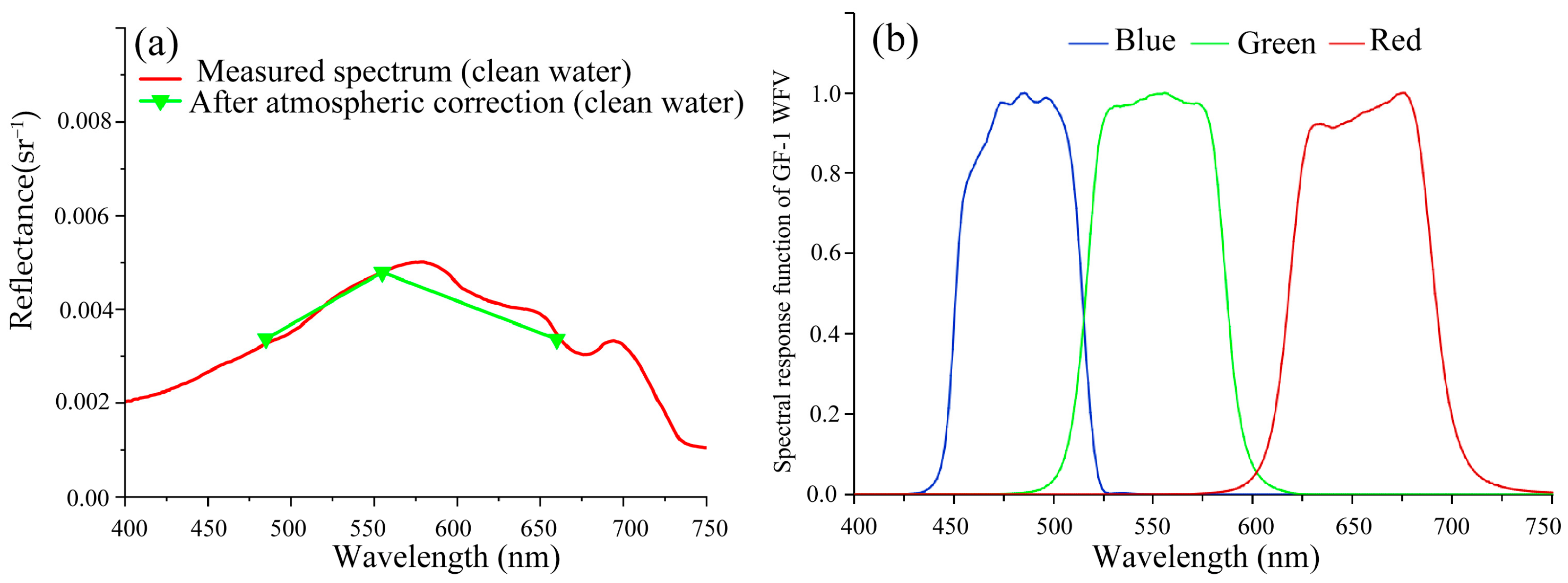
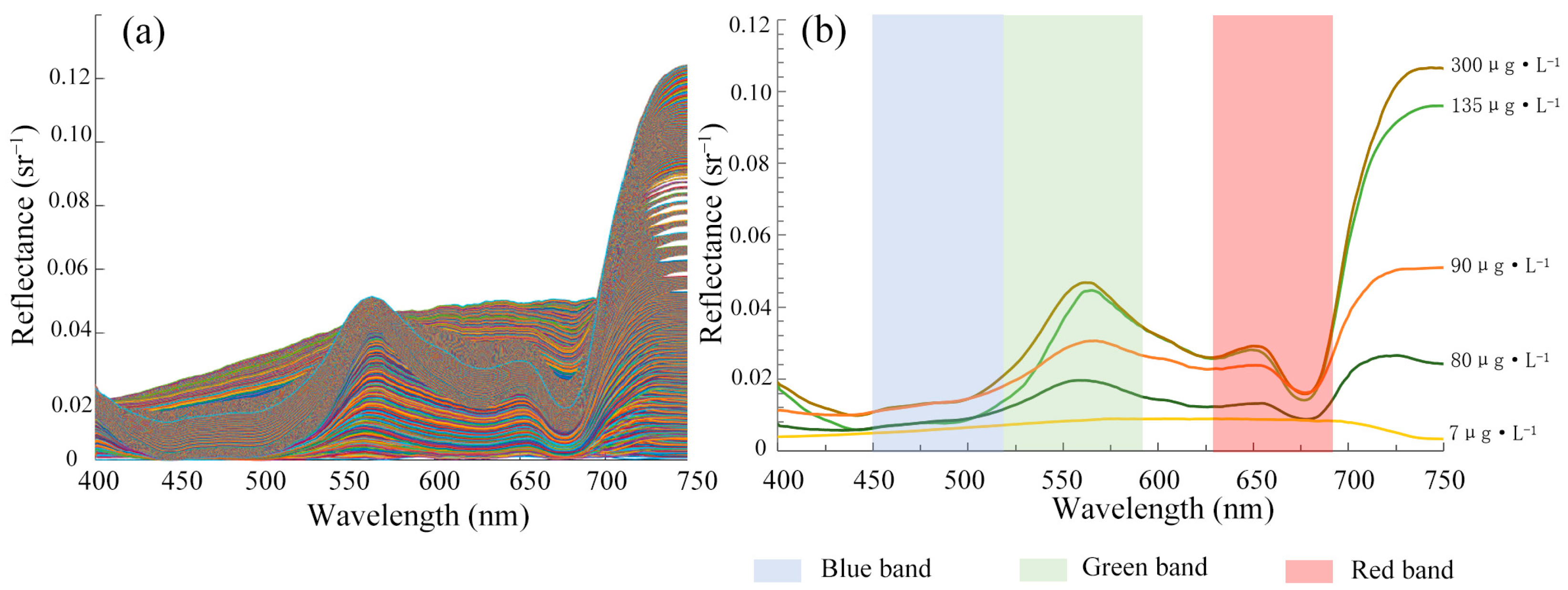
Above-Water Spectral Reflectance Measurements

Above-water radiance measurements were performed vertically above the water surface at an azimuth angle of 135° using an ASD FieldSpec 4 Hi-Res spectroradiometer, covering a wavelength range of 350 to 2500 nm. Approximately 10 measurements were averaged to yield the final upwelling radiance spectrum, with the sun-glint spectrum excluded [40]. The skylight radiance spectrum was measured when the ASD spectroradiometer sensor viewed the sky at a zenith angle of 40°. Additionally, the downwelling radiance spectrum was measured vertically on a Lambertian Spectralon plate (called a “Grey Plate”) with a reflectance factor of 30%.

2.1.4. GF-1 WFV Data

The GF-1 satellite was launched on 26 April 2013. The four WFV sensors have a combined swath width of nearly 800 km, covering four wavelengths (blue: 0.45–0.52 μm; green: 0.52–0.59 μm; red: 0.63–0.69 μm; near-infrared radiation (NIR): 0.77–0.89 μm) with a spatial resolution of 16 m and a temporal resolution of 2–4 days. The GF-1 WFV data can be downloaded from the China Center for Resources Satellite Data and Application (CRESDA), which currently provides level 1 GF-1 data, at https://data.cresda.cn/#/home (accessed on 16 November 2024). The WFV datasets obtained on 23 August 2024 and used in this paper were radiometrically calibrated using the calibration coefficients released by CRESDA, further calibrated with in situ measurements from the clear water area, and atmospherically corrected using the traditional fast line-of-sight atmospheric analysis of spectral hypercubes (FLAASH) method (Figure 2a). Each visible band was smooth filtered with a 7 × 7 sliding window to reduce the image noise. The spectral response functions in visible bands of the GF-1 WFV datasets, illustrated in Figure 2b, were convolved with the subsequent hyperspectral datasets, including absorption coefficients, backscattering coefficients, and both upwelling and downwelling attenuation coefficients.

2.2. Methodology

2.2.1. Identifying the Emergent Aquatic Plants/Submerged Aquatic Plants

Numerous emergent aquatic plants are typically exposed above the water, and a large area of submerged aquatic plants and bottom mud are also noted. The water signals beneath the emergent aquatic plants cannot be detected by satellites. However, the overlying water of the submerged aquatic plants or bottom mud can effectively reveal the water quality of the water body, representing an important part of the lake environment. Therefore, it is necessary to distinguish and separate the area of the emergent aquatic plants from the area of submerged aquatic plants or bottom mud. An identification model and algorithm for distinguishing the submerged aquatic plants from the emergent aquatic plants based on the NDVI are presented as follows:

$$\mathrm{B}\mathrm{o}\mathrm{t}\mathrm{t}\mathrm{o}\mathrm{m} \mathrm{l}\mathrm{a}\mathrm{n}\mathrm{d} \mathrm{c}\mathrm{o}\mathrm{v}\mathrm{e}\mathrm{r}=\left\{\begin{array}{c}\mathrm{E}\mathrm{m}\mathrm{e}\mathrm{r}\mathrm{g}\mathrm{e}\mathrm{n}\mathrm{t}\mathrm{a}\mathrm{q}\mathrm{u}\mathrm{a}\mathrm{t}\mathrm{i}\mathrm{c}\mathrm{p}\mathrm{l}\mathrm{a}\mathrm{n}\mathrm{t}\mathrm{s},\mathrm{N}\mathrm{D}\mathrm{V}\mathrm{I}\ge 0.52\\ \mathrm{s}\mathrm{u}\mathrm{b}\mathrm{m}\mathrm{e}\mathrm{r}\mathrm{g}\mathrm{e}\mathrm{d}\mathrm{a}\mathrm{q}\mathrm{u}\mathrm{a}\mathrm{t}\mathrm{i}\mathrm{c}\mathrm{p}\mathrm{l}\mathrm{a}\mathrm{n}\mathrm{t}\mathrm{s},-0.46\le \mathrm{N}\mathrm{D}\mathrm{V}\mathrm{I}<0.52\\ \mathrm{m}\mathrm{u}\mathrm{d},\mathrm{N}\mathrm{D}\mathrm{V}\mathrm{I}<-0.46\end{array}\right.$$

(1)

The formula used for NDVI calculations is expressed as follows:

$$\mathrm{N}\mathrm{D}\mathrm{V}\mathrm{I}={\displaystyle \frac{\mathrm{N}\mathrm{I}\mathrm{R}-\mathrm{R}\mathrm{E}\mathrm{D}}{\mathrm{N}\mathrm{I}\mathrm{R}+\mathrm{R}\mathrm{E}\mathrm{D}}}$$

(2)

where RED and NIR represent the red band and near-infrared band reflectance of the GF1 WFV data, respectively.

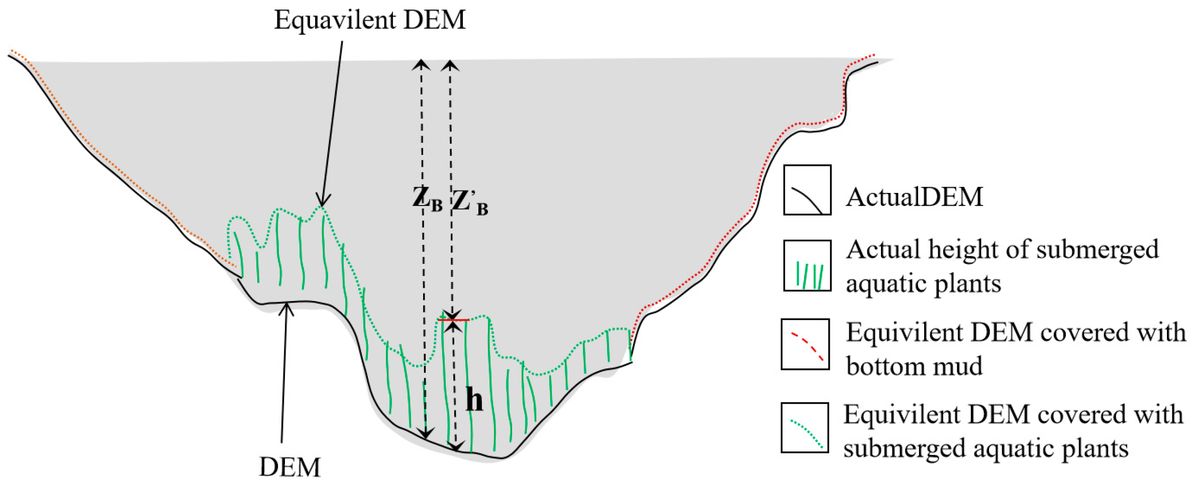
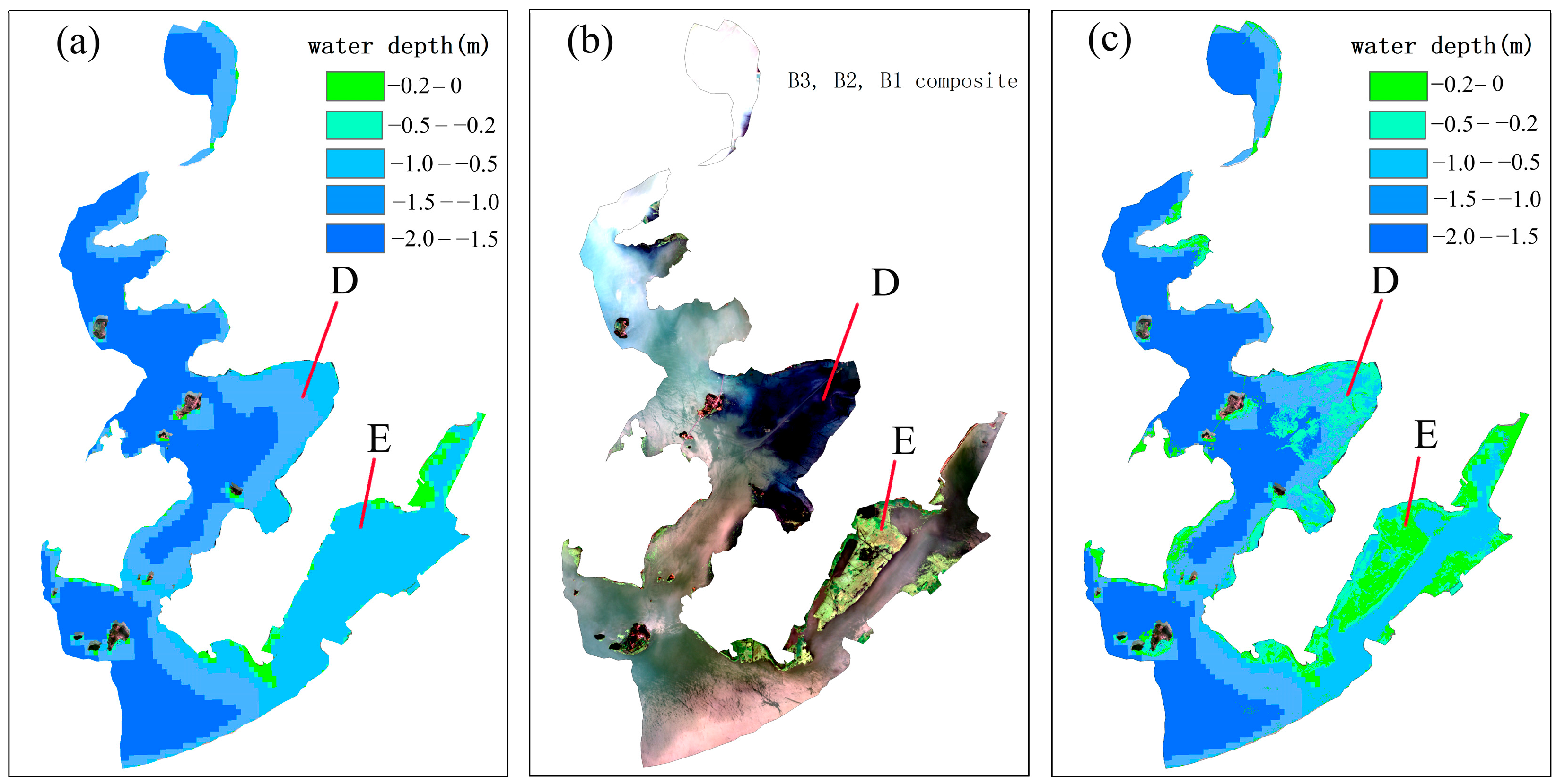
2.2.2. Water Depth-Optimized Bottom Effect Removal Method

The closer the top of a plant is to the surface, the greater the contribution of aquatic plants to the reflectance spectra [30,31]. Thus, the different h values of the submerged aquatic plants growing on the bottom (${\mathrm{Z}}_{\mathrm{B}}$) are equivalent to the actual underwater digital elevation model (DEM) patched with a terrain of h. In other words, the equivalent water depth ${\mathrm{Z}}_{\mathrm{B}}^{\prime }$ (${\mathrm{Z}}_{\mathrm{B}}^{\prime }$ = ${\mathrm{Z}}_{\mathrm{B}}$ − h) is the combination of the actual ${\mathrm{Z}}_{\mathrm{B}}$ with the h of the submerged aquatic plants (Figure 3).

According to Lee et al. (1998) [25], the remote sensing reflectance just below the water surface in optically shallow waters is affected by water depth, bottom albedo, and diffuse attenuation coefficients. The subsurface remote sensing reflectance with the bottom effect removed is typically described using the radiative transfer process as follows:

$${\mathrm{r}}_{\mathrm{r}\mathrm{s},\mathrm{m}\mathrm{u}\mathrm{d} \mathrm{o}\mathrm{r} \mathrm{s}\mathrm{u}\mathrm{b}\mathrm{m}\mathrm{e}\mathrm{r}\mathrm{g}\mathrm{e}\mathrm{d} \mathrm{p}\mathrm{l}\mathrm{a}\mathrm{n}\mathrm{t}}^{\mathrm{d}\mathrm{p}}={\displaystyle \frac{{\mathrm{R}}_{\mathrm{r}\mathrm{s}}-\left(1.562{\mathrm{R}}_{\mathrm{r}\mathrm{s}}+0.518\right){\mathrm{A}}_1\mathsf{\rho }\mathrm{e}\mathrm{x}\mathrm{p}\left\{-({\mathrm{K}}_{\mathrm{d}}+{\mathrm{K}}_{\mathrm{u}}^{\mathrm{B}}){\mathrm{Z}}_{\mathrm{B}}\right\}}{\left[0.518+1.562{\mathrm{R}}_{\mathrm{r}\mathrm{s}}\right]\left[1-{\mathrm{A}}_0\mathrm{e}\mathrm{x}\mathrm{p}\left\{-\left({\mathrm{K}}_{\mathrm{d}}+{\mathrm{K}}_{\mathrm{u}}^{\mathrm{c}}\right)\right.\left.{\mathrm{Z}}_{\mathrm{B}}\right\}\right]}}$$

(3)

where ${\mathrm{R}}_{\mathrm{r}\mathrm{s}}$ represents the above-water remote sensing reflectance; ${\mathrm{r}}_{\mathrm{r}\mathrm{s}}^{\mathrm{d}\mathrm{p}}$ is the subsurface remote reflectance for optically deep waters; ${\mathrm{K}}_{\mathrm{d}}$ is the vertically diffuse attenuation coefficients for downwelling irradiance; ${\mathrm{K}}_{\mathrm{u}}^{\mathrm{c}}$ is the vertically diffuse attenuation coefficients for upwelling irradiance from the water column; ${\mathrm{K}}_{\mathrm{u}}^{\mathrm{B}}$ is the vertically diffuse attenuation coefficients for upwelling irradiance from the bottom; $\mathsf{\rho }$ is the irradiance reflectance of the bottom as a Lambertian reflector; and ${\mathrm{A}}_0$ = 1.03 and ${\mathrm{A}}_1$ = 0.31 were determined by comparing the hydrolight-calculated ${\mathrm{r}}_{\mathrm{r}\mathrm{s}}$ with that of the proposed semi-analytical model [25].

Generally speaking, the water depth and the chlorophyll-a concentrations in the area of submerged aquatic plants should be the same or similar to that of waters nearby, such as adjacent waters without submerged aquatic plant coverage. The diverse reflectance spectra in this area can mainly be ascribed to the varying h values of the submerged plants. According to Formula (3), the pixels that are influenced by the submerged aquatic plants are uniformly assigned with the pixel values of the adjacent waters of bottom mud coverage. Then, the optimized ${\mathrm{Z}}_{\mathrm{B}}^{\prime }$ can be calculated using the following formula:

$${\mathrm{r}}_{\mathrm{r}\mathrm{s},\mathrm{i}}^{\mathrm{a}\mathrm{d}\mathrm{j}\mathrm{a}\mathrm{c}\mathrm{e}\mathrm{n}\mathrm{t} \mathrm{p}\mathrm{i}\mathrm{x}\mathrm{e}\mathrm{l} \mathrm{o}\mathrm{f} \mathrm{b}\mathrm{o}\mathrm{t}\mathrm{t}\mathrm{o}\mathrm{m} \mathrm{m}\mathrm{u}\mathrm{d}}={\displaystyle \frac{{\mathrm{R}}_{\mathrm{r}\mathrm{s},\mathrm{i}}-(1.562{\mathrm{R}}_{\mathrm{r}\mathrm{s},\mathrm{i}}+0.518){\mathrm{A}}_1{\mathsf{\rho }}_{\left(\mathrm{i}\right)}\mathrm{e}\mathrm{x}\mathrm{p}\left\{-({\mathrm{K}}_{\mathrm{d},\mathrm{i}}+{\mathrm{K}}_{\mathrm{u},\mathrm{i}}^{\mathrm{B}}){\mathrm{Z}}_{\mathrm{B}}^{\prime }\right\}}{[0.518+1.562{\mathrm{R}}_{\mathrm{r}\mathrm{s},\mathrm{i}}][1-{\mathrm{A}}_0\mathrm{e}\mathrm{x}\mathrm{p}\left\{-({\mathrm{K}}_{\mathrm{d},\mathrm{i}}+{\mathrm{K}}_{\mathrm{u},\mathrm{i}}^{\mathrm{C}}){\mathrm{Z}}_{\mathrm{B}}^{\prime }\right\}]}}\left(\mathrm{i}=\mathrm{B}\mathrm{l}\mathrm{u}\mathrm{e},\mathrm{G}\mathrm{r}\mathrm{e}\mathrm{e}\mathrm{n} \mathrm{o}\mathrm{r} \mathrm{R}\mathrm{e}\mathrm{d} \mathrm{b}\mathrm{a}\mathrm{n}\mathrm{d}\right)$$

(4)

The obtained optimized value of ${\mathrm{Z}}_{\mathrm{B}}^{\prime }$ can be substituted into the original Equation (3), and the ${\mathrm{r}}_{\mathrm{r}\mathrm{s},\mathrm{m}\mathrm{u}\mathrm{d} \mathrm{o}\mathrm{r} \mathrm{u}\mathrm{n}\mathrm{d}\mathrm{e}\mathrm{r}\mathrm{w}\mathrm{a}\mathrm{t}\mathrm{e}\mathrm{r} \mathrm{p}\mathrm{l}\mathrm{a}\mathrm{n}\mathrm{t}}^{\mathrm{d}\mathrm{p}}$ is the remote sensing reflectance just beneath the water surface with the water depth-optimized bottom effect removed. The remote sensing reflectance, ${\mathrm{R}}_{\mathrm{r}\mathrm{s}}\left(\mathrm{i}\right)$, above the water surface of the multi-spectral bands with the bottom effect removed can be expressed as follows:

$${\mathrm{R}}_{\mathrm{r}\mathrm{s}}\left(\mathrm{i}\right)\approx {\displaystyle \frac{0.518{\mathrm{r}}_{\mathrm{r}\mathrm{s},\mathrm{i}}^{\mathrm{B}\mathrm{o}\mathrm{t}\mathrm{t}\mathrm{o}\mathrm{m} \mathrm{E}\mathrm{f}\mathrm{f}\mathrm{e}\mathrm{c}\mathrm{t} \mathrm{R}\mathrm{e}\mathrm{m}\mathrm{o}\mathrm{v}\mathrm{a}\mathrm{l}}}{1-1.562{\mathrm{r}}_{\mathrm{r}\mathrm{s},\mathrm{i}}^{\mathrm{B}\mathrm{o}\mathrm{t}\mathrm{t}\mathrm{o}\mathrm{m} \mathrm{E}\mathrm{f}\mathrm{f}\mathrm{e}\mathrm{c}\mathrm{t} \mathrm{R}\mathrm{e}\mathrm{m}\mathrm{o}\mathrm{v}\mathrm{a}\mathrm{l}}}};\left(\mathrm{i}=\mathrm{B}\mathrm{l}\mathrm{u}\mathrm{e},\mathrm{G}\mathrm{r}\mathrm{e}\mathrm{e}\mathrm{n} \mathrm{o}\mathrm{r} \mathrm{R}\mathrm{e}\mathrm{d} \mathrm{b}\mathrm{a}\mathrm{n}\mathrm{d}\right)$$

(5)

Therefore, under conditions where the irradiance reflectance spectrum of the underwater substrate, the upwelling and downwelling irradiance attenuation coefficients, and the water depth are known, it is possible to obtain the blue, green, and red band reflectance spectra of the water body in the optically shallow water with the bottom effect removed.

2.2.3. Spectral Matching-Based Chlorophyll-a Retrieval Method

The spectral (400–750 nm) reflectance model presented by Gordon et al. [41] is adapted to Taihu Lake to better interpret our in situ measurements. Specifically, it is used to explain the influence of the bottom effect of submerged aquatic plants on ${\mathrm{R}}_{\mathrm{r}\mathrm{s}}$ and to estimate the chlorophyll-a concentrations in phytoplankton in optically shallow waters.

Remote sensing reflectance spectra above water are related to the concentrations of water constituents (chlorophyll-a, detritus, and yellow substances) and the specific inherent optical properties (SIOPs) as noted by Bricaud et al. (1995) [42]:

$${\mathrm{R}}_{\mathrm{r}\mathrm{s}}\left(\mathsf{\lambda }\right)={\displaystyle \frac{0.182}{\mathrm{Q}}}·{\displaystyle \frac{{\mathrm{b}}_{\mathrm{w}}+{\mathrm{C}}_{\mathrm{T}\mathrm{S}\mathrm{M}}·{\mathrm{b}}_{\mathrm{b}\mathrm{p}}^{\ast }\left(\mathsf{\lambda }\right)}{{\mathrm{a}}_{\mathrm{w}}+{\mathrm{C}}_{\mathrm{p}\mathrm{h}}·{\mathrm{a}}_{\mathrm{p}\mathrm{h}}^{\ast }\left(\mathsf{\lambda }\right)+{\mathrm{C}}_{\mathrm{d}}·{\mathrm{a}}_{\mathrm{d}}^{\ast }\left(\mathsf{\lambda }\right)+{\mathrm{a}}_{\mathrm{y}}\left(440\right)·\exp \left(0.011\left(\mathsf{\lambda }-440\right)\right)+{\mathrm{b}}_{\mathrm{w}}+{\mathrm{C}}_{\mathrm{T}\mathrm{S}\mathrm{M}}·{\mathrm{b}}_{\mathrm{b}\mathrm{p}}^{\ast }\left(\mathsf{\lambda }\right)}}$$

(6)

where ${\mathrm{R}}_{\mathrm{r}\mathrm{s}}$ represents the above-water remote sensing reflectance; a_w denotes the absorption coefficient of pure water referenced from Deng Ruru et al. [43]; ${\mathrm{a}}_{\mathrm{p}\mathrm{h}}^{\ast }(\mathsf{\lambda })$ is the specific absorption coefficient of phytoplankton pigments; ${\mathrm{C}}_{\mathrm{p}\mathrm{h}}$ is the chlorophyll-a concentration in phytoplankton ($\mathsf{\mu }{\mathrm{g}·\mathrm{L}}^{-1}$); ${\mathrm{a}}_{\mathrm{d}}^{\ast }\left(\mathsf{\lambda }\right)$ is the specific absorption coefficient of detritus (non-algal particles); ${\mathrm{C}}_{\mathrm{d}}$ is the concentration of detritus ($\mathrm{m}{\mathrm{g}·\mathrm{L}}^{-1}$); ${\mathrm{a}}_{\mathrm{y}}\left(440\right)$ is the absorption coefficient at 440 nm; b_bw represents the backscattering coefficient of pure water cited by Smith and Baker [44]; and ${\mathrm{b}}_{\mathrm{b}\mathrm{p}}^{\ast }(\mathsf{\lambda })$ is the specific backscattering coefficient of the total suspended matter. The weight of the total suspended matter ${\mathrm{C}}_{\mathrm{T}\mathrm{S}\mathrm{M}}$ includes the dry weight of detritus (non-algal particles) and phytoplankton (algal particles), and the dry weight of phytoplankton is correlated with the chlorophyll-a concentration. According to Hoogenboom et al. [45], ${\mathrm{C}}_{\mathrm{T}\mathrm{S}\mathrm{M}}={\mathrm{C}}_{\mathrm{d}}+0.07·{\mathrm{C}}_{\mathrm{p}\mathrm{h}}$.

Based on the SIOPs, the spectral curves of different concentrations of the water constituents can be simulated using the reflectance model, and a spectral library of different spectral curves of known concentrations of Taihu water constituents was established.

Spectral matching involves comparing the reflectance spectra (in situ hyperspectral or satellite multi-spectral bands) of a target water body with those of known concentrations of water constituents in a spectral library. The formula for spectral matching is expressed as follows:

$${\mathrm{D}}^2=\sum ({\mathrm{R}}_{\mathrm{r}\mathrm{s}}^{\mathrm{m}\mathrm{e}\mathrm{a}\mathrm{s}\mathrm{u}\mathrm{r}\mathrm{e}\mathrm{d}}(\mathsf{\lambda })-{\mathrm{R}}_{\mathrm{r}\mathrm{s}}^{\mathrm{s}\mathrm{p}\mathrm{e}\mathrm{c}\mathrm{t}\mathrm{r}\mathrm{a}\mathrm{l} \mathrm{l}\mathrm{i}\mathrm{b}\mathrm{r}\mathrm{a}\mathrm{r}\mathrm{y}}(\mathsf{\lambda }){)}^2$$

(7)

where ${\mathrm{R}}_{\mathrm{r}\mathrm{s}}^{\mathrm{m}\mathrm{e}\mathrm{a}\mathrm{s}\mathrm{u}\mathrm{r}\mathrm{e}\mathrm{d}}(\mathsf{\lambda })$ represents the reflectance of the target water body obtained using in situ measurements or the multi-spectral images obtained from the satellite imaging system; ${\mathrm{R}}_{\mathrm{r}\mathrm{s}}^{\mathrm{s}\mathrm{p}\mathrm{e}\mathrm{c}\mathrm{t}\mathrm{r}\mathrm{a}\mathrm{l} \mathrm{l}\mathrm{i}\mathrm{b}\mathrm{r}\mathrm{a}\mathrm{r}\mathrm{y}}(\mathsf{\lambda })$ represents the reflectance spectrum of known concentrations of water constituents in the spectral library; and $\sum ()$ represents the sum over all bands. Once the most matched spectrum is identified, the concentration (such as chlorophyll-a) can be calculated.

2.2.4. Accuracy Assessment Metrics

For the established classification model, accuracy, precision, and recall are utilized as evaluation metrics to assess its performance. The calculation formulas are as follows:

$$\mathrm{A}\mathrm{c}\mathrm{c}\mathrm{u}\mathrm{r}\mathrm{a}\mathrm{c}\mathrm{y}={\displaystyle \frac{\mathrm{T}\mathrm{P}+\mathrm{T}\mathrm{N}}{\mathrm{T}\mathrm{P}+\mathrm{T}\mathrm{N}+\mathrm{F}\mathrm{P}+\mathrm{F}\mathrm{N}}}$$

(8)

$$\mathrm{P}\mathrm{r}\mathrm{e}\mathrm{c}\mathrm{i}\mathrm{s}\mathrm{i}\mathrm{o}\mathrm{n}={\displaystyle \frac{\mathrm{T}\mathrm{P}}{\mathrm{T}\mathrm{P}+\mathrm{F}\mathrm{P}}}$$

(9)

$$\mathrm{R}\mathrm{e}\mathrm{c}\mathrm{a}\mathrm{l}\mathrm{l}={\displaystyle \frac{\mathrm{T}\mathrm{P}}{\mathrm{T}\mathrm{P}+\mathrm{F}\mathrm{N}}}$$

(10)

where True Positive (TP) represents the number of samples that are actually positive and are correctly predicted as positive by the model; True Negative (TN) denotes the number of samples that are actually negative and are correctly predicted as negative by the model; False Positive (FP) indicates the number of samples that are actually negative but are incorrectly predicted as positive by the model; and False Negative (FN) refers to the number of samples that are actually positive but are erroneously predicted as negative by the model.

3. Results

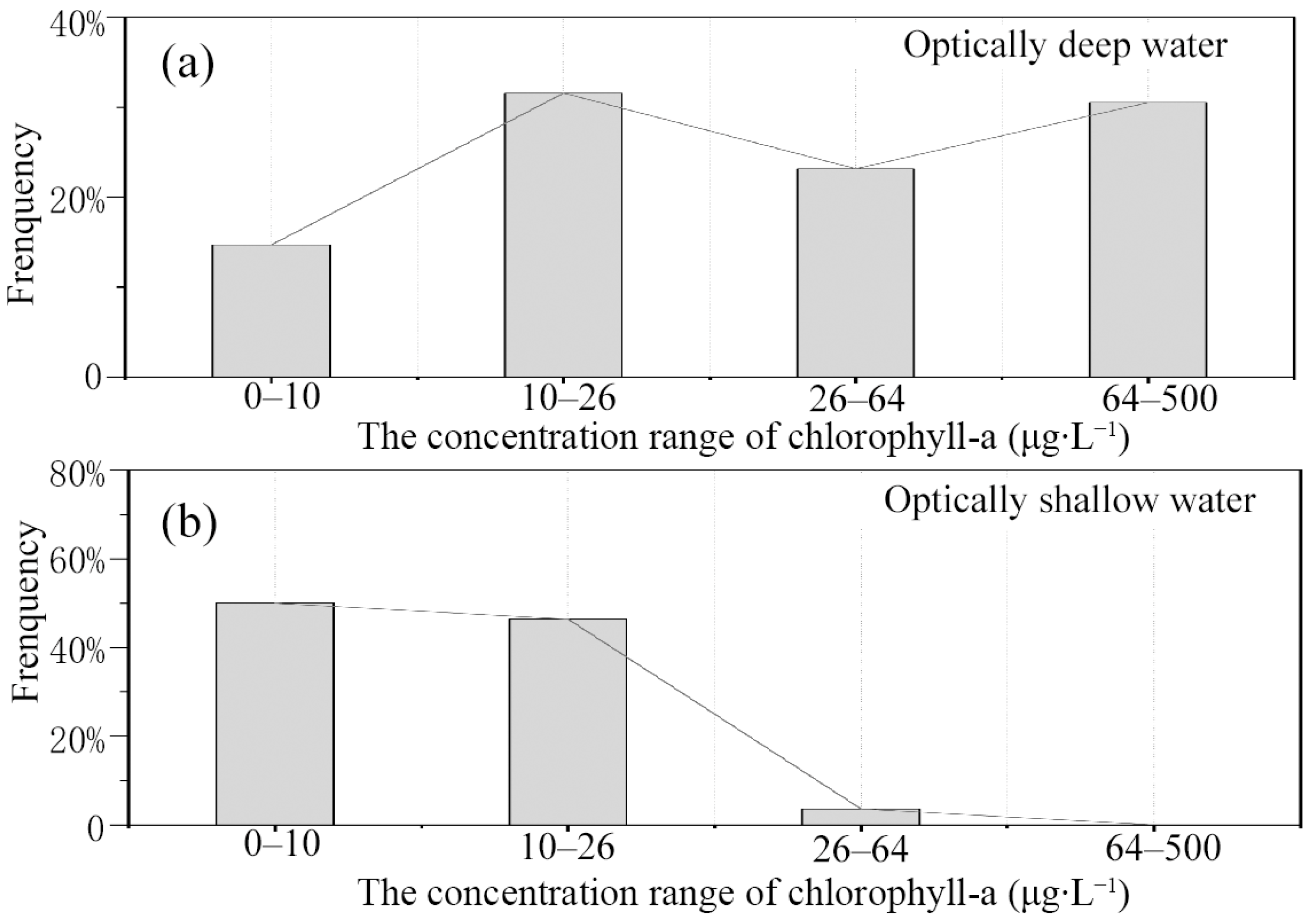
3.1. In Situ Chlorophyll-a Concentrations

The in situ surface chlorophyll-a concentrations (n = 146) measured during the past four cruises ranged from 2 to 495 $\mathsf{\mu }{\mathrm{g}·\mathrm{L}}^{-1}$. Obvious differences in phytoplankton chlorophyll-a concentrations are noted between the western part and the eastern part of Taihu Lake. Western Taihu Lake, which is characterized by optically deep waters, is typically eutrophic with chlorophyll-a concentrations between 2 and 495 $\mathsf{\mu }{\mathrm{g}·\mathrm{L}}^{-1}$, whereas eastern Taihu, which is characterized by optically shallow waters, is oligotrophic to mesotrophic with chlorophyll-a concentrations between 2 and 28 $\mathsf{\mu }{\mathrm{g}·\mathrm{L}}^{-1}$ (Figure 4). The boundary between the optically deep waters and the optically shallow waters can change dynamically due to wind-induced bottom mud resuspension. Algal scums rarely reach the far end of the optically shallow waters, where the submerged aquatic plants grow.

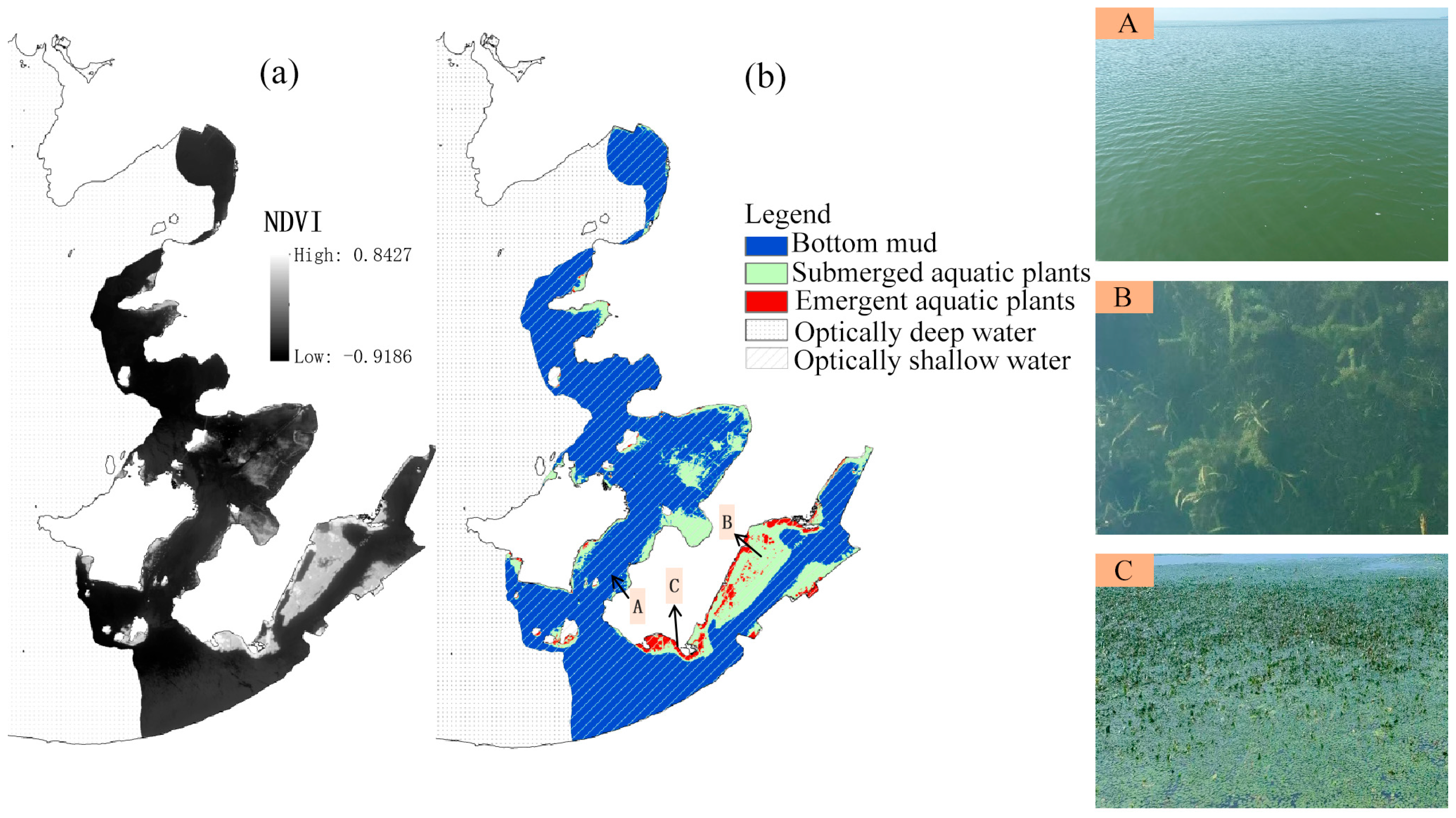
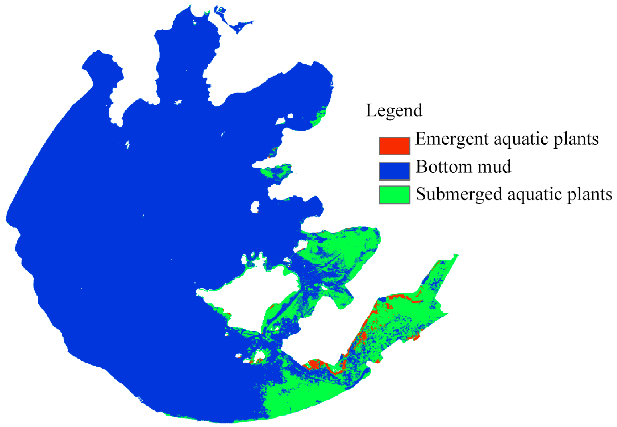
3.2. Identification of Emergent Aquatic Plants and Submerged Aquatic Plants

The spectra of submerged aquatic plants vary. The closer they are to the water surface, the more they present spectral characteristics similar to those of above-water vegetation, and the spectra of submerged aquatic plants at different depths vary greatly [30,31]. Figure 5 provides the remote sensing reflectance spectra of submerged aquatic plants and bottom mud (0.02 m from the water surface to the top of the aquatic submerged plant or bottom mud) measured just beneath the water surface (0⁻). Because the upwelling radiance attenuation coefficients of different bands vary with wavelengths, the attenuation in the near-infrared band is higher than that in the red band. The NDVI of underwater vegetation is significantly lower than that of emergent aquatic plants, and it can be used to distinguish emergent aquatic plants from underwater vegetation.

In order to classify the substrate land cover in optically shallow waters in eastern Taihu Lake, the empirical thresholds for each class (bottom mud, submerged aquatic plants, and emergent plants) were determined by calculating the arithmetic mean of a 9 × 9 window centered at the sampling location on the NDVI image. Here, the maximum NDVI pixel value, ${\mathrm{N}\mathrm{D}\mathrm{V}\mathrm{I}}_{\mathrm{m}\mathrm{u}\mathrm{d}}^{\mathrm{m}\mathrm{a}\mathrm{x}\mathrm{i}\mathrm{m}\mathrm{u}\mathrm{m}}$, of six bottom mud samples (the remaining three bottom mud samples were used for validation), the minimum and maximum ${(\mathrm{N}\mathrm{D}\mathrm{V}\mathrm{I}}_{\mathrm{s}\mathrm{u}\mathrm{b}\mathrm{m}\mathrm{e}\mathrm{r}\mathrm{g}\mathrm{e}\mathrm{d} \mathrm{a}\mathrm{q}\mathrm{u}\mathrm{a}\mathrm{t}\mathrm{i}\mathrm{c} \mathrm{p}\mathrm{l}\mathrm{a}\mathrm{n}\mathrm{t}\mathrm{s}}^{\mathrm{m}\mathrm{i}\mathrm{n}\mathrm{i}\mathrm{m}\mathrm{u}\mathrm{m}}$ and ${\mathrm{N}\mathrm{D}\mathrm{V}\mathrm{I}}_{\mathrm{s}\mathrm{u}\mathrm{b}\mathrm{m}\mathrm{e}\mathrm{r}\mathrm{g}\mathrm{e}\mathrm{d} \mathrm{a}\mathrm{q}\mathrm{u}\mathrm{a}\mathrm{t}\mathrm{i}\mathrm{c} \mathrm{p}\mathrm{l}\mathrm{a}\mathrm{n}\mathrm{t}\mathrm{s}}^{\mathrm{m}\mathrm{a}\mathrm{x}\mathrm{i}\mathrm{m}\mathrm{u}\mathrm{m}}$) NDVI pixel values of 14 samples of submerged aquatic plants (the remaining five samples of submerged aquatic plants were used for validation), and the minimum NDVI values of emergent aquatic plants at the six sites (${\mathrm{N}\mathrm{D}\mathrm{V}\mathrm{I}}_{\mathrm{e}\mathrm{m}\mathrm{e}\mathrm{r}\mathrm{g}\mathrm{e}\mathrm{n}\mathrm{t} \mathrm{p}\mathrm{l}\mathrm{a}\mathrm{n}\mathrm{t}\mathrm{s}}^{\mathrm{m}\mathrm{i}\mathrm{n}\mathrm{i}\mathrm{m}\mathrm{u}\mathrm{m}}$) (the remaining two emergent plant samples were used for validation) are noted. The empirical thresholds were slightly adjusted and finally confirmed using visual evaluation of the classification. The substrate land cover types are identified as follows: emergent aquatic plants when NDVI ≥ 0.52, submerged aquatic plants when −0.46 ≤ NDVI < 0.52, and bottom mud when NDVI < −0.46.

According to Equation (1), the classification of the bottom land cover types in the eastern part of Lake Taihu is illustrated in Figure 6 using NDVI images from GF-1 WFV datasets obtained on 23 August 2024. The confusion matrix shows that the six bottom mud samples and six emergent plant samples were correctly classified, whereas one out of 14 submerged aquatic plant samples was classified incorrectly. Thus, the performance of the classification model can be evaluated using the confusion matrix, with the results shown below (

Table 2. The confusion matrix of bottom land cover classification.

		Classification
Ground truth		Bottom Mud	Submerged Aquatic Plants	Emergent Plants
	Bottom mud	6	0	0
	Submerged aquatic plants	0	13	1
	Emergent aquatic plants	0	0	6

).

The model achieved a True Positive (TP) count of 13, a True Negative (TN) count of 12, a False Positive (FP) count of 0, and a False Negative (FN) count of 1. Consequently, the model demonstrated an accuracy of 96%, a precision of 100%, and a recall of 92%.

Finally, the classification results were validated using the remaining 10 samples (three bottom mud samples, five submerged aquatic plant samples, and two emergent plant samples) with an accuracy of 90% (with one submerged aquatic plant sample misclassified as an emergent plant).

Given that Taihu Lake is characterized by highly turbid waters due to the wind-driven resuspension of sediments, the extent of the shallow optical waters can change drastically, which may result in an incomplete mapping of the submerged aquatic plants using a single scene from a remote sensing image. The middle- to high-resolution remote sensing images from past cruises, like the Landsat 5 TM image obtained on 28 October 2003, the Sentinel 2 image obtained on 30 October 2023, and the GF-1 WFV image obtained on 23 August 2024, were combined to extract the submerged aquatic plants (Figure 7).

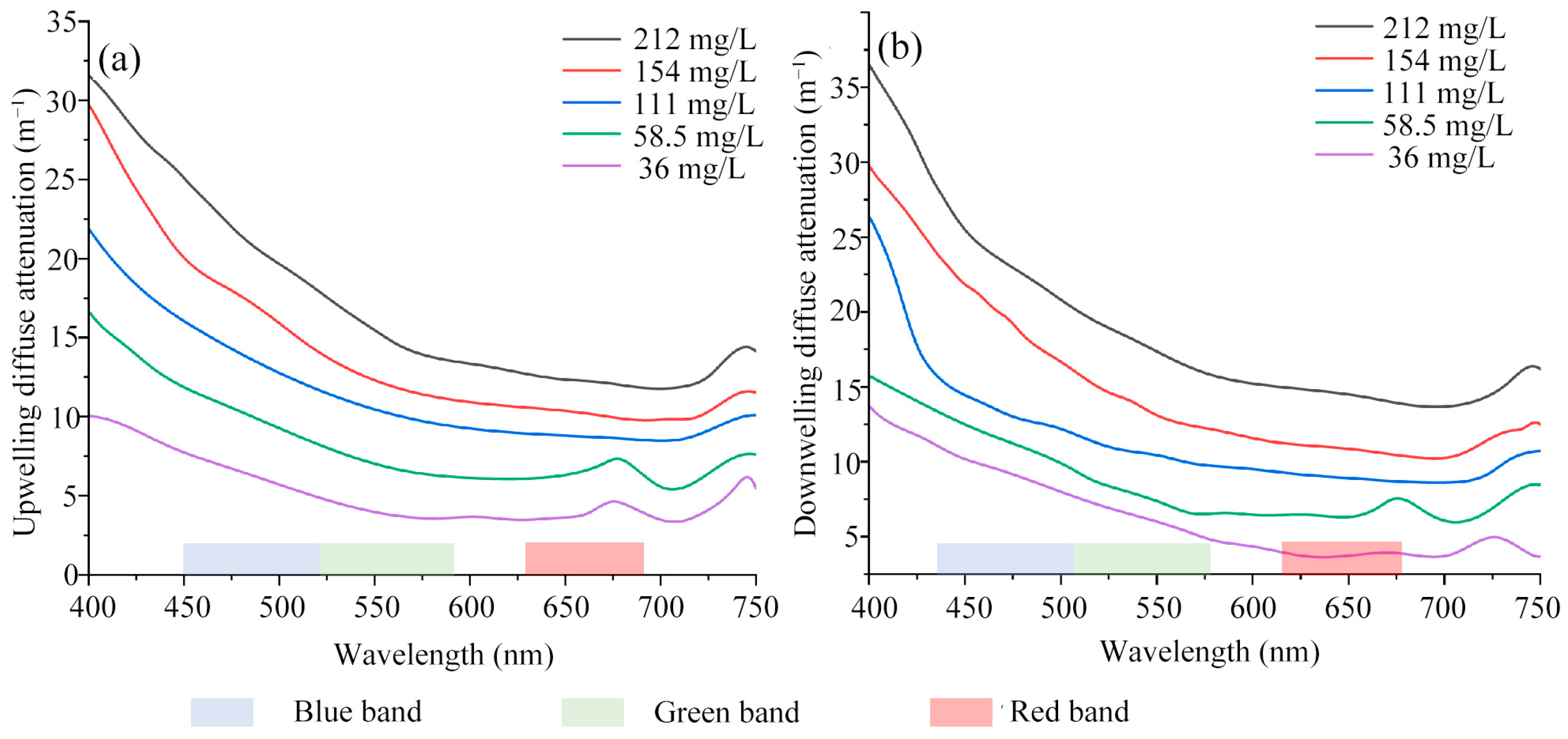
3.3. Upwelling and Downwelling Diffuse Attenuation Coefficients

Underwater downwelling irradiance, upwelling irradiance, and upwelling radiance measurements were performed every 10 cm from 0 (just below the air–water surface, $0^{-}$) to 1.0 m using the Irradian SR9910-computer-controlled spectroradiometer with a wavelength range of 350–850 nm. The irradiance attenuation of the underwater light field follows an exponential attenuation:

$${\mathrm{K}}_{\mathrm{d}}=-{\displaystyle \frac{1}{\mathrm{z}}}\mathrm{l}\mathrm{n}{\displaystyle \frac{\mathrm{E}\left(\mathrm{Z}\right)}{\mathrm{E}\left(0^{-}\right)}}$$

(11)

where ${\mathrm{K}}_{\mathrm{d}}$ is the diffuse attenuation coefficient, z is the depth from the water surface to the measurement point, $\mathrm{E}(\mathrm{z})$ is the irradiance at a water depth of z, and $\mathrm{E}(0^{-})$ is the irradiance just below the water surface ${(0}^{-})$. ${\mathrm{K}}_{\mathrm{d}}$ was obtained by an exponential function fitting of the irradiances at different depths (number of depths (N) > 5, ${\mathrm{R}}^2$ > 0.95).

Lake Taihu is a typical highly turbid inland water characterized by sediment resuspension. The apparent and inherent optical properties of the water body, as well as the optical radiative transfer in the water, are all closely related to the concentration of the suspended sediment. Figure 8 shows the downwelling and upwelling irradiance attenuation coefficients at different suspended sediment concentrations. The upwelling and downwelling attenuation coefficients were processed using a convolution with the spectral response functions (in Figure 2) of the GF-1 WFV datasets. It can be seen that both the downwelling and upwelling irradiance attenuation coefficients decrease significantly as the wavelength increases within the range of 400–700 nm. When the wavelength is greater than 700 nm, the downwelling and upwelling irradiance attenuation coefficients gradually increase. This is related to the strong absorption of pure water. Notably, the downwelling and upwelling irradiance attenuation coefficients show approximately equal intervals, indicating that the upwelling and downwelling irradiance attenuation coefficients have a good linear correlation with the suspended sediment concentrations in the range of the blue, green, and red bands of the GF-1 satellite (Figure 8). This makes it possible to retrieve the upwelling and downwelling attenuation coefficients using the suspended sediment concentrations.

Numerous studies on the remote sensing algorithms for the suspended sediment have been performed [46,47,48,49]. For the GF-1 WFV image with a resolution of 16 m, the suspended sediment concentration inversion algorithm is as follows (${\mathrm{R}}^2=0.76$, root mean square error (RMSE) = 8.53 $\mathrm{m}{\mathrm{g}·\mathrm{L}}^{-1}$) [50]:

$${\mathrm{C}}_{\mathrm{T}\mathrm{S}\mathrm{S}}=119.62\ast {\left({\displaystyle \frac{\mathrm{b}3}{\mathrm{b}2}}\right)}^{6.0823}$$

(12)

where TSS represents the concentration of total suspended sediments (${\mathrm{m}\mathrm{g}·\mathrm{L}}^{-1}$), and b2 and b3 are the atmospheric-corrected radiance values of the respective green band and red band of the GF-1 WFV image.

According to Lee et al. (1998) [25], the upwelling attenuation coefficients of bottom ${\mathrm{K}}_{\mathrm{u}}^{\mathrm{B}}$ are related to the upwelling attenuation coefficients of column ${\mathrm{K}}_{\mathrm{u}}^{\mathrm{C}}$ based on a function of inherent optical properties:

$${\mathrm{K}}_{\mathrm{u}}^{\mathrm{B}}={\mathrm{K}}_{\mathrm{u}}^{\mathrm{C}}·\sqrt{{\displaystyle \frac{1.44\left(1+2.0\frac{{\mathrm{b}}_{\mathrm{b}}}{\mathrm{a}+{\mathrm{b}}_{\mathrm{b}}}\right)}{1.21\left(1+4.9\frac{{\mathrm{b}}_{\mathrm{b}}}{\mathrm{a}+{\mathrm{b}}_{\mathrm{b}}}\right)}}}$$

(13)

A linear function is used to fit the upwelling and downwelling diffuse attenuation coefficients with concentrations of the suspended sediments in the visible bands of the GF-1 WFV datasets. Here, the ${\mathrm{R}\mathrm{M}\mathrm{S}\mathrm{E}}_{\mathrm{d}\mathrm{o}\mathrm{w}\mathrm{n}\mathrm{w}\mathrm{e}\mathrm{l}\mathrm{l}\mathrm{i}\mathrm{n}\mathrm{g} \mathrm{a}\mathrm{t}\mathrm{t}\mathrm{e}\mathrm{n}\mathrm{u}\mathrm{a}\mathrm{t}\mathrm{i}\mathrm{o}\mathrm{n}}$ values for the blue, green, and red bands were 3.13 ${\mathrm{m}}^{-1}$, 2.07 ${\mathrm{m}}^{-1}$, and 1.65 ${\mathrm{m}}^{-1}$, respectively. The ${\mathrm{M}\mathrm{A}\mathrm{P}\mathrm{E}}_{\mathrm{d}\mathrm{o}\mathrm{w}\mathrm{n}\mathrm{w}\mathrm{e}\mathrm{l}\mathrm{l}\mathrm{i}\mathrm{n}\mathrm{g} \mathrm{a}\mathrm{t}\mathrm{t}\mathrm{e}\mathrm{n}\mathrm{u}\mathrm{a}\mathrm{t}\mathrm{i}\mathrm{o}\mathrm{n}}$ values for the blue, green, and red bands were 16.07%, 15.10%, and 13.85%, respectively. The ${\mathrm{R}\mathrm{M}\mathrm{S}\mathrm{E}}_{\mathrm{u}\mathrm{p}\mathrm{w}\mathrm{e}\mathrm{l}\mathrm{l}\mathrm{i}\mathrm{n}\mathrm{g} \mathrm{a}\mathrm{t}\mathrm{t}\mathrm{e}\mathrm{n}\mathrm{u}\mathrm{a}\mathrm{t}\mathrm{i}\mathrm{o}\mathrm{n}}^{\mathrm{C}}$ values for the blue, green, and red bands were 2.85 ${\mathrm{m}}^{-1}$, 1.94 ${\mathrm{m}}^{-1}$, and 1.53 ${\mathrm{m}}^{-1}$, respectively, and the ${\mathrm{M}\mathrm{A}\mathrm{P}\mathrm{E}}_{\mathrm{u}\mathrm{p}\mathrm{w}\mathrm{e}\mathrm{l}\mathrm{l}\mathrm{i}\mathrm{n}\mathrm{g} \mathrm{a}\mathrm{t}\mathrm{t}\mathrm{e}\mathrm{n}\mathrm{u}\mathrm{a}\mathrm{t}\mathrm{i}\mathrm{o}\mathrm{n}}^{\mathrm{C}}$ values for the blue, green, and red bands were 15.01%, 14.78%, and 13.60%, respectively. The ${\mathrm{R}\mathrm{M}\mathrm{S}\mathrm{E}}_{\mathrm{u}\mathrm{p}\mathrm{w}\mathrm{e}\mathrm{l}\mathrm{l}\mathrm{i}\mathrm{n}\mathrm{g} \mathrm{a}\mathrm{t}\mathrm{t}\mathrm{e}\mathrm{n}\mathrm{u}\mathrm{a}\mathrm{t}\mathrm{i}\mathrm{o}\mathrm{n}}^{\mathrm{B}}$ values for the blue, green, and red bands were 0.46 ${\mathrm{m}}^{-1}$, 0.28 ${\mathrm{m}}^{-1}$, and 0.26 ${\mathrm{m}}^{-1}$, respectively, and the ${\mathrm{M}\mathrm{A}\mathrm{P}\mathrm{E}}_{\mathrm{u}\mathrm{p}\mathrm{w}\mathrm{e}\mathrm{l}\mathrm{l}\mathrm{i}\mathrm{n}\mathrm{g} \mathrm{a}\mathrm{t}\mathrm{t}\mathrm{e}\mathrm{n}\mathrm{u}\mathrm{a}\mathrm{t}\mathrm{i}\mathrm{o}\mathrm{n}}^{\mathrm{B}}$ values for the blue, green, and red bands were 13.50%, 12.08%, and 10.53%, respectively. The specific algorithms are provided in

Table 3. The linear functions of downwelling (K_d) and upwelling (${\mathrm{K}}_{\mathrm{u}}^{\mathrm{C}}$ and ${\mathrm{K}}_{\mathrm{u}}^{\mathrm{B}}$) diffuse attenuation coefficients with suspended sediments in the visible bands of the GF-1 WFV datasets.

	Formula	RMSE (m−1)	MAPE	Formula	RMSE (m−1)	MAPE	Formula	RMSE (m−1)	MAPE
Blue	${\mathrm{K}}_{\mathrm{d},\mathrm{B}\mathrm{l}\mathrm{u}\mathrm{e}}$ = 0.078 × TSS + 3.717	3.13	16.07%	${\mathrm{K}}_{\mathrm{u},\mathrm{B}\mathrm{l}\mathrm{u}\mathrm{e}}^{\mathrm{C}}$ = 0.081 × TSS + 2.678	2.85	15.01%	${\mathrm{K}}_{\mathrm{u},\mathrm{B}\mathrm{l}\mathrm{u}\mathrm{e}}^{\mathrm{B}}$ = 0.084 × TSS + 3.938	0.46	13.50%
Green	${\mathrm{K}}_{\mathrm{d},\mathrm{G}\mathrm{r}\mathrm{e}\mathrm{e}\mathrm{n}}$ = 0.059 × TSS + 2.226	2.07	15.10%	${\mathrm{K}}_{\mathrm{u},\mathrm{G}\mathrm{r}\mathrm{e}\mathrm{e}\mathrm{n}}^{\mathrm{C}}$ = 0.058 × TSS + 1.880	1.94	14.78%	${\mathrm{K}}_{\mathrm{u},\mathrm{G}\mathrm{r}\mathrm{e}\mathrm{e}\mathrm{n}}^{\mathrm{B}}$ = 0.062 × TSS + 1.972	0.28	12.08%
Red	${\mathrm{K}}_{\mathrm{d},\mathrm{R}\mathrm{e}\mathrm{d}}$ = 0.046 × TSS + 2.474	1.65	13.85%	${\mathrm{K}}_{\mathrm{u},\mathrm{R}\mathrm{e}\mathrm{d}}^{\mathrm{C}}$ = 0.042 × TSS + 2.449	1.53	13.60%	${\mathrm{K}}_{\mathrm{u},\mathrm{R}\mathrm{e}\mathrm{d}}^{\mathrm{B}}$ = 0.04 × TSS + 3.546	0.26	10.53%

Here, TSS represents the concentration of total suspended sediments (${\mathrm{m}\mathrm{g}·\mathrm{L}}^{-1}$), ${\mathrm{K}}_{\mathrm{d}}$ is the downwelling irradiance attenuation coefficient (${\mathrm{m}}^{-1}$), ${\mathrm{K}}_{\mathrm{u}}^{\mathrm{C}}$ is the upwelling irradiance attenuation coefficient of the water column (${\mathrm{m}}^{-1}$), and ${\mathrm{K}}_{\mathrm{u}}^{\mathrm{B}}$ is the upwelling irradiance attenuation coefficient of the bottom (${\mathrm{m}}^{-1}$).

.

3.4. Performance of the Spectral Reflectance Model with the Bottom Effect Removed

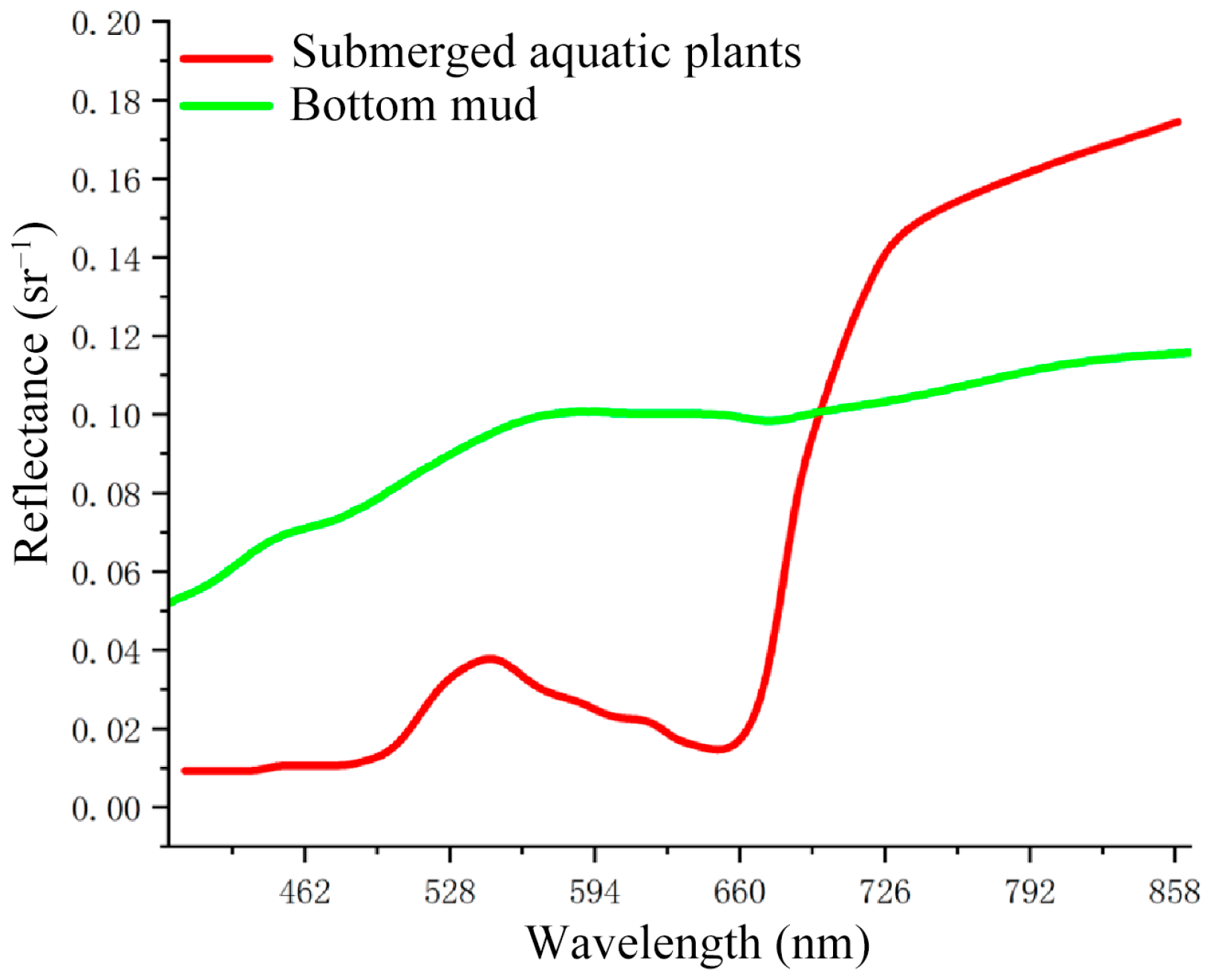
3.4.1. Spectral Library for Taihu Lake

The mean absorption coefficients of detritus a_d(λ), phytoplankton a_ph(λ), yellow substances a_y(λ), and pure water a_w(λ) and the specific absorption coefficients of detritus ${\mathrm{a}}_{\mathrm{d}}^{\ast }(\mathsf{\lambda })$ and phytoplankton ${\mathrm{a}}_{\mathrm{p}\mathrm{h}}^{\ast }(\mathsf{\lambda })$ in the range of the visible bands are shown in Figure 9.

The absorption coefficient of detritus approaches zero near 750 nm and decreases exponentially with increasing wavelength in the range of 400–750 nm. A negative exponential model is adopted to model the absorption coefficient of non-pigment particles ${\mathrm{a}}_{\mathrm{d}}(\mathsf{\lambda })$ as follows:

$${\mathrm{a}}_{\mathrm{d}}\left(\mathsf{\lambda }\right)={\mathrm{a}}_{\mathrm{d}}\left(440\right)\times \mathrm{e}\mathrm{x}\mathrm{p}\left(0.0123\times \left(440-\mathsf{\lambda }\right)\right)$$

(14)

The absorption coefficient of yellow substances is similar to that of non-pigmented particles, showing an exponential decay trend, as shown in Equation (15).

$${\mathrm{a}}_{\mathrm{y}}\left(\mathsf{\lambda }\right)={\mathrm{a}}_{\mathrm{y}}\left(440\right)\times \mathrm{e}\mathrm{x}\mathrm{p}\left(0.011\times \left(440-\mathsf{\lambda }\right)\right)$$

(15)

The absorption spectra of phytoplankton illustrate two diagnostic absorption peaks, in the blue band (approximately 430–440 nm) and in the red band (approximately 675 nm).

The total absorption spectra were similar to those of the detritus, indicating the intense absorption in the detritus-dominated highly turbid inland waters.

The specific absorption coefficients of detritus in the blue, green, and red bands of the GF-1 WFV datasets were 0.053 ${\mathrm{m}}^2·{\mathrm{m}\mathrm{g}}^{-1}$, 0.022 ${\mathrm{m}}^2·{\mathrm{m}\mathrm{g}}^{-1}$, and 0.008 ${\mathrm{m}}^2·{\mathrm{m}\mathrm{g}}^{-1}$, respectively.

The specific absorption coefficients of phytoplankton, which decrease with increasing chlorophyll-a concentrations, exhibit an obvious “package effect”. The specific absorption coefficients of phytoplankton in the blue, green, and red bands of the GF-1 WFV datasets were 0.045 ${\mathrm{m}}^2·{\mathsf{\mu }\mathrm{g}}^{-1}$, 0.017 ${\mathrm{m}}^2·{\mathsf{\mu }\mathrm{g}}^{-1}$, and 0.018 ${\mathrm{m}}^2·{\mathsf{\mu }\mathrm{g}}^{-1}$, respectively.

The mean backscattering coefficients and the specific backscattering coefficients in the range of the visible bands are illustrated in Figure 10.

The backscattering coefficients of total suspended particles are highly correlated with the concentrations of detritus in the visible bands. The mean backscattering coefficients showed a decrease with increasing wavelengths in the visible bands, which is consistent with that reported by Forget et al. (1999) [51]. The specific backscattering coefficients for the blue, green, and red bands of the GF-1 WFV datasets were 0.112 ${\mathrm{m}}^2·{\mathrm{m}\mathrm{g}}^{-1}$, 0.107 ${\mathrm{m}}^2·{\mathrm{m}\mathrm{g}}^{-1}$, and 0.087 ${\mathrm{m}}^2·{\mathrm{m}\mathrm{g}}^{-1}$, respectively.

According to Equation (6), given the SIOPs, the spectral curve of certain concentrations of the water constituents can be simulated using the reflectance model. Thus, according to the specific absorption coefficients in Figure 9 and the specific backscattering coefficients in Figure 10, the spectral curves of different concentrations of water constituents in the range of 400–750 nm were simulated. Chlorophyll-a ranged from 2 to 400 $\mathsf{\mu }{\mathrm{g}·\mathrm{L}}^{-1}$ with an interval of 1 $\mathsf{\mu }{\mathrm{g}·\mathrm{L}}^{-1}$. The TSS concentration ranged from 1 to 300 $\mathrm{m}{\mathrm{g}·\mathrm{L}}^{-1}$ with an interval of 5 $\mathrm{m}{\mathrm{g}·\mathrm{L}}^{-1}$. CDOM absorption at 440 nm varied from 0.50 to 4.0 ${\mathrm{m}}^{-1}$ with an interval of 0.2 ${\mathrm{m}}^{-1}$. Therefore, there are a total of 462,441 (399 × 61 × 19) spectral curves of known concentrations of water constituents in the spectral library (Figure 11a), and the spectral characteristics of different chlorophyll-a concentrations are significantly different from each other (Figure 11b).

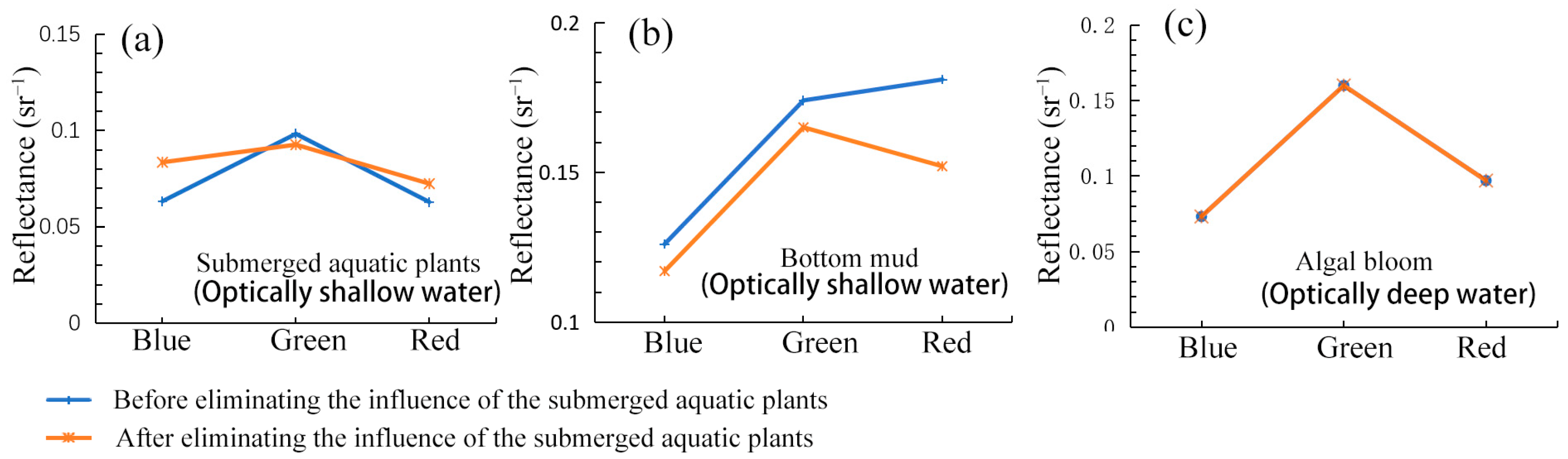
3.4.2. Water Depth-Optimized Bottom Effect Removal

Water depth optimization is a method used to adjust for the varied heights of submerged aquatic plants relative to the actual water depth. Compared to the actual water depth, the optimized water depth method presents more detailed water depth data characterized by distinct varied heights of submerged aquatic plants in the eastern part of Taihu Lake (Figure 12). The actual water depth ${\mathrm{Z}}_{\mathrm{B}}$ in area D (Xukou Town) is approximately 1.0–1.6 m, and the optimized water depth ${\mathrm{Z}}_{\mathrm{B}}^{\prime }$ in area D is approximately 0.50–0.20 m, accounting for only 12.5–50% of the actual water depth. This implies that the submerged aquatic plants are 0.7–1.4 m high in area D. In contrast, ${\mathrm{Z}}_{\mathrm{B}}$ in area E (Linhu Town) is approximately 1.0 m or less, and ${\mathrm{Z}}_{\mathrm{B}}^{\prime }$ in area E is approximately 0–0.20 m, accounting for only 0–20% of the actual water depth. This also implies that the submerged aquatic plants are 0.8–1.0 m tall in area E. Although the heights of the submerged aquatic plants in area D may be taller than those of area E, the difference in ${\mathrm{Z}}_{\mathrm{B}}^{\prime }$ at the two sites is the main cause for the significant differences in the spectra or textures in the true color composite image obtained from the GF-1 WFV datasets on 23 August 2024. The smaller the ${\mathrm{Z}}_{\mathrm{B}}^{\prime }$ value (the closer the top of the submerged plants to the water surface), the greater the bottom effect of aquatic plants on the reflectance spectra.

Using the optimized water depth (${\mathrm{Z}}_{\mathrm{B}}^{\prime }$) in the radiative transfer process, we can conduct quantitative assessments and eliminate the bottom effect of submerged aquatic plants in optically shallow waters. In the area of submerged aquatic plants, the reflectance spectra processed using the water depth-optimized bottom effect removal method exhibit the following features. For the blue band characterized by the strong absorption of chlorophyll-a in submerged aquatic plants, the reflectance spectrum increases significantly. For the green band characterized by strong “green reflection” of the underwater vegetation, the reflectance spectrum decreases. For the red band characterized by strong absorption of chlorophyll-a in submerged aquatic plants, the reflectance spectrum increases to a certain extent (Figure 13a). In the area of bottom mud, the reflectance spectra processed using the water depth-optimized bottom effect removal method exhibit the following features. For the blue band, the contribution of the bottom mud is removed, and the reflectance spectrum decreases slightly. For the green band, the reflectance spectrum decreases slightly. For the red band, the reflectance spectrum decreases moderately (Figure 13b). In optically deep water where the bottom effect is minimal, the spectral reflectance remains unchanged before and after processing using this water depth-optimized bottom effect removal method (Figure 13c).

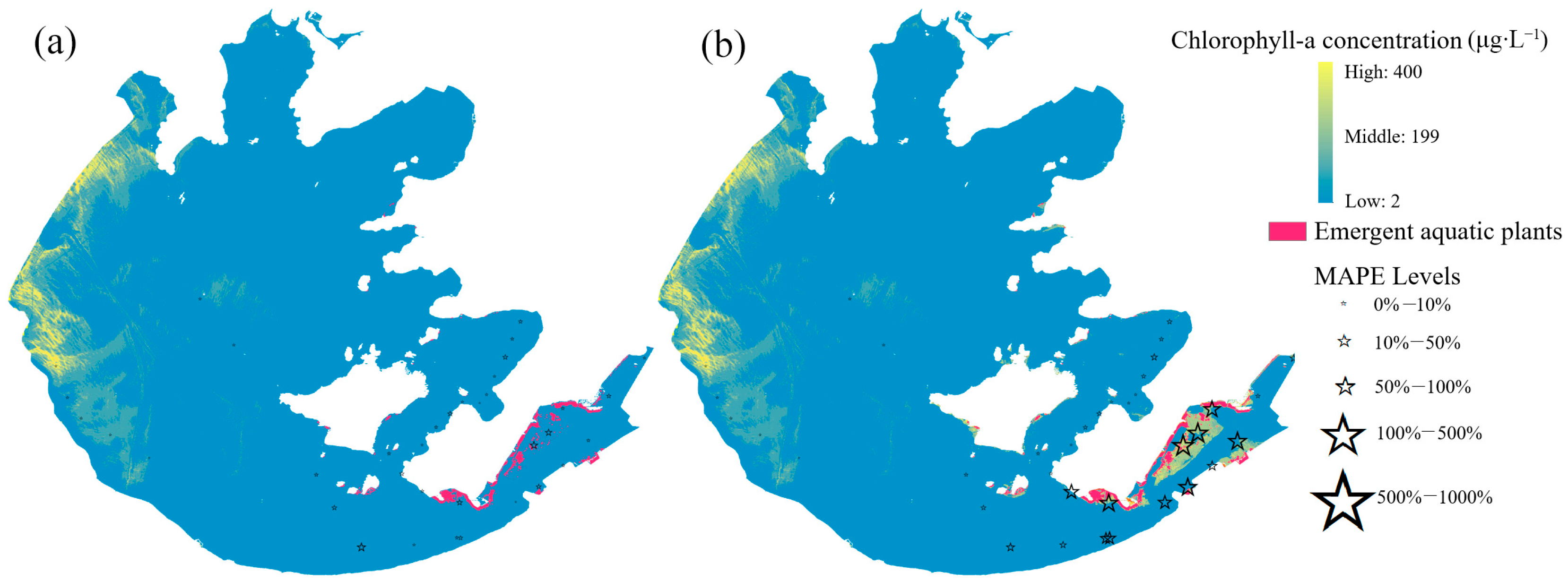
3.4.3. Chlorophyll-a Retrieval in Taihu Lake

The chlorophyll-a concentrations in optically complex Taihu waters (including the optically deep and optically shallow waters) were retrieved using the spectral matching methods with the GF-1 WFV visible bands (red, green, and blue) obtained on 23 August 2024. The chlorophyll-a concentrations in phytoplankton obtained using the traditional retrieval algorithm (retrieving model by using the GF-1 WFV datasets without the water depth-optimized bottom effect removed) are overestimated in the area with numerous submerged aquatic plants in the eastern part of Taihu Lake, whereas the chlorophyll-a concentrations in phytoplankton obtained using the proposed algorithm (the same retrieving model by using the GF-1 WFV datasets with the water depth-optimized bottom effect removed) are fairly low. These findings are consistent with the field data (Figure 14).

The absolute error for the samples below 7–8 $\mathsf{\mu }{\mathrm{g}·\mathrm{L}}^{-1}$ is relatively small in the extremely eutrophic Taihu Lake. Moreover, for the samples with high concentrations of suspended solids, the measurement error for their low chlorophyll-a concentrations is relatively large. Therefore, the samples with extremely low concentrations are excluded, and only samples with chlorophyll-a levels greater than 8 $\mathsf{\mu }{\mathrm{g}·\mathrm{L}}^{-1}$ are statistically analyzed. The quantitative results also showed that the proposed reflectance model with the bottom effect removed can achieve ±19.58% mean absolute percentage error (MAPE) (RMSE = 8.69 $\mathsf{\mu }{\mathrm{g}·\mathrm{L}}^{-1}$) compared to the traditional retrieval algorithm without eliminating the bottom effect with a MAPE of ±245.12% (RMSE = 45.61 $\mathsf{\mu }{\mathrm{g}·\mathrm{L}}^{-1}$) (Figure 14 and Figure 15,

Table 4. Comparison of chlorophyll-a concentrations obtained with/without the bottom effect removed.

Chlorophyll-a	RMSE	MAPE
Obtained using the bottom effect removal method	8.69 $\mathsf{\mu }{\mathrm{g}·\mathrm{L}}^{-1}$	19.58%
Obtained without using the bottom effect removal method	45.61 $\mathsf{\mu }{\mathrm{g}·\mathrm{L}}^{-1}$	245.12%

).

Validation

Further authenticity tests were performed using the field data obtained on 24 August 2024. The validation results show that the chlorophyll-a concentration retrieved using the retrieving model with the bottom effect removal method exhibits good consistency with the measured data (RMSE = 10.89 $\mathsf{\mu }{\mathrm{g}·\mathrm{L}}^{-1}$, MAPE = 17.52%).

4. Discussion

During the monitoring of cyanobacterial blooms using remote sensing, submerged aquatic plants contribute significantly to the water-leaving radiance. This will lead to an overestimation of chlorophyll-a concentrations in optically shallow waters. Researchers have proposed algorithms to simultaneously determine the chlorophyll-a concentration, water depth, bottom albedo, and inherent optical property parameters [25,26,27,28]. On the basis of these optical radiation transfer models in optically shallow water, Albert et al. (2003) [29] developed new parameterizations of the irradiance reflectance and the remote sensing reflectance for case 2 waters of Lake Constance, and Cannizzaro et al. (2006) [52] proposed several empirical ocean chlorophyll-a retrieval algorithms in oceanic regions containing different bottom reflectance contributions. The contribution of submerged aquatic plants to the reflectance spectrum varies greatly in different regions, and the closer the top of the submerged plants to the water surface, the greater the bottom effect of aquatic plants on the reflectance spectra [30,31]. As a further development of the optically shallow water radiative transfer model, this paper quantitatively analyzes the significant differences between the actual water depth and the optimized water depth characterized by the varying h values of submerged aquatic plants. It is not the actual water depth ${\mathrm{Z}}_{\mathrm{B}}$ but rather the equivalent ${\mathrm{Z}}_{\mathrm{B}}^{\prime }$ (${\mathrm{Z}}_{\mathrm{B}}^{\prime }$ = ${\mathrm{Z}}_{\mathrm{B}}$ − h) that affects the contribution of the submerged aquatic plants to the water-leaving signals. Consequently, the proposed chlorophyll-a concentration estimation algorithm based on the water depth-optimized bottom effect removal method efficiently reduces the bottom effect of the submerged aquatic plants.

Although we validated the retrieval of chlorophyll-a concentrations in phytoplankton with high accuracy in the eastern part of Taihu Lake, there are still some uncertainties that could be improved in future studies. In the section on water depth optimization, as a theoretical assumption, the inherent optical properties and actual water depth of the submerged aquatic plant pixels are considered to be the same as or similar to those of the nearest bottom mud pixels. This is highly probable but is not always true. In certain extreme circumstances, such as at the interface between two water bodies with significantly different water depths or different inherent optical properties, this assumption could introduce large errors. In the section on spectral library simulation, the specific absorption coefficients and specific backscattering coefficients of different water constituents adopted in spectral curve simulation are simple approximations of the actual inherent optical properties, and it has not reflected the actual seasonal changes of the inherent optical properties yet. In the section of chlorophyll-a retrieval by spectral matching, it is a roughly, not an exact minimum distance ${\mathrm{D}}^2$ that defined to measure the matching degree between the measured spectra of the target water and the simulated spectra in the spectral library. All the uncertainties mentioned above may result in an error propagation in retrieving chlorophyll-a concentrations in phytoplankton.

The chlorophyll-a concentrations in phytoplankton across the whole of Lake Taihu, including the optically deep waters in western Taihu and the optically shallow waters in eastern Taihu, can be computed and validated with high accuracy. This method of chlorophyll-a concentration retrieval is highly local and seasonal and still has certain limitations when applied to other water bodies.

5. Conclusions

Due to the bottom effect of submerged aquatic plants, retrieving chlorophyll-a concentrations in phytoplankton in optically shallow waters can lead to overestimations and incorrect eutrophication evaluations. This study leveraged the water depth-optimized bottom effect removal method and the spectral matching-based chlorophyll-a retrieval method to accurately retrieve chlorophyll-a concentrations in phytoplankton in optically complex water bodies. The main findings are as follows:

(1)

A method based on the NDVI can categorize the underwater land cover types into three categories: underwater aquatic plants (−0.46 ≤ NDVI < 0.52), emergent aquatic plants or floating-leaved plants (NDVI ≥ 0.52), and the bottom mud (NDVI < −0.46). Through visual inspection and field verification, the accuracy of the results is greater than 90%;

(2)

The characteristics of the downwelling and upwelling irradiance attenuation coefficients were discussed. The remote sensing-based retrieval models for the downwelling irradiance attenuation coefficients in the three visible bands yielded the following results. The RMSE values for the blue, green, and red bands were 3.13 ${\mathrm{m}}^{-1}$, 2.07 ${\mathrm{m}}^{-1}$, and 1.65 ${\mathrm{m}}^{-1}$, respectively. The MAPE values for the blue, green, and red bands were 16.07%, 15.10%, and 13.85%, respectively. The upwelling irradiance attenuation coefficients (${\mathrm{R}\mathrm{M}\mathrm{S}\mathrm{E}}_{\mathrm{u}\mathrm{p}\mathrm{w}\mathrm{e}\mathrm{l}\mathrm{l}\mathrm{i}\mathrm{n}\mathrm{g} \mathrm{a}\mathrm{t}\mathrm{t}\mathrm{e}\mathrm{n}\mathrm{u}\mathrm{a}\mathrm{t}\mathrm{i}\mathrm{o}\mathrm{n}}^{\mathrm{C}}$) were 2.85 ${\mathrm{m}}^{-1}$, 1.94 ${\mathrm{m}}^{-1}$, and 1.53 ${\mathrm{m}}^{-1}$, for the blue, green, and red bands, respectively, and the ${\mathrm{M}\mathrm{A}\mathrm{P}\mathrm{E}}_{\mathrm{u}\mathrm{p}\mathrm{w}\mathrm{e}\mathrm{l}\mathrm{l}\mathrm{i}\mathrm{n}\mathrm{g} \mathrm{a}\mathrm{t}\mathrm{t}\mathrm{e}\mathrm{n}\mathrm{u}\mathrm{a}\mathrm{t}\mathrm{i}\mathrm{o}\mathrm{n}}^{\mathrm{C}}$ values for the blue, green, and red bands were 15.01%, 14.78%, and 13.60%, respectively. The ${\mathrm{R}\mathrm{M}\mathrm{S}\mathrm{E}}_{\mathrm{u}\mathrm{p}\mathrm{w}\mathrm{e}\mathrm{l}\mathrm{l}\mathrm{i}\mathrm{n}\mathrm{g} \mathrm{a}\mathrm{t}\mathrm{t}\mathrm{e}\mathrm{n}\mathrm{u}\mathrm{a}\mathrm{t}\mathrm{i}\mathrm{o}\mathrm{n}}^{\mathrm{B}}$ values for the blue, green, and red bands were 0.46 ${\mathrm{m}}^{-1}$, 0.28 ${\mathrm{m}}^{-1}$, and 0.26 ${\mathrm{m}}^{-1}$, respectively, and the ${\mathrm{M}\mathrm{A}\mathrm{P}\mathrm{E}}_{\mathrm{u}\mathrm{p}\mathrm{w}\mathrm{e}\mathrm{l}\mathrm{l}\mathrm{i}\mathrm{n}\mathrm{g} \mathrm{a}\mathrm{t}\mathrm{t}\mathrm{e}\mathrm{n}\mathrm{u}\mathrm{a}\mathrm{t}\mathrm{i}\mathrm{o}\mathrm{n}}^{\mathrm{B}}$ values for the blue, green, and red bands were 13.50%, 12.08%, and 10.53%, respectively;

(3)

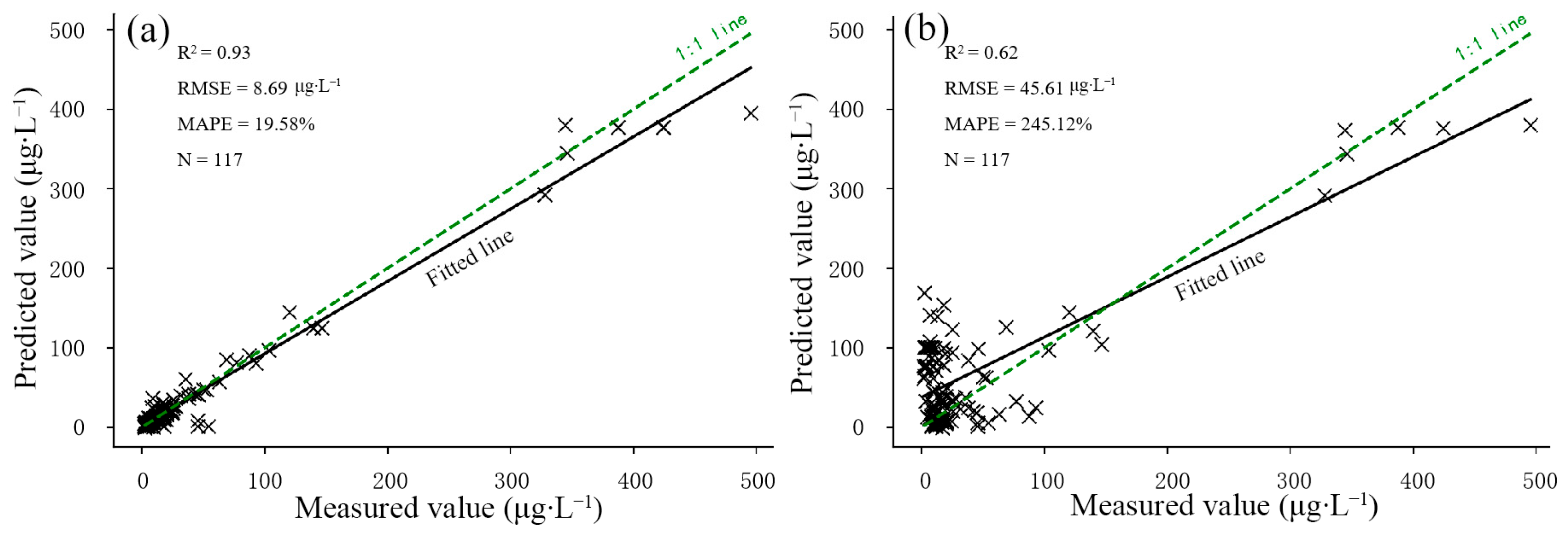
A chlorophyll-a concentration estimation algorithm based on the bottom effect removal method using a water depth optimization approach is proposed, yielding a MAPE of ±19.58% and RMSE of 8.69 $\mathsf{\mu }{\mathrm{g}·\mathrm{L}}^{-1}$. These values are superior to those of the traditional algorithm without bottom effect removal with a MAPE of ±245.12% and RMSE of 45.61 $\mathsf{\mu }{\mathrm{g}·\mathrm{L}}^{-1}$. The validation yields an accuracy of ±17.52% for MAPE and 10.89 $\mathsf{\mu }{\mathrm{g}·\mathrm{L}}^{-1}$ for RMSE, which is consistent with the proposed algorithm.

References

1. Ogashawara, I.; Mishra, D.R.; Gitelson, A.A. Remote Sensing of Inland Waters: Background and Current State-of-the-Art. In Bio-Optical Modeling and Remote Sensing of Inland Waters; Elsevier: Amsterdam, The Netherlands, 2017; pp. 1–24. ISBN 978-0-12-804654-8. [Google Scholar]
2. Lehmann, M.K.; Gurlin, D.; Pahlevan, N.; Alikas, K.; Anstee, J.; Balasubramanian, S.V.; Barbosa, C.C.F.; Binding, C.; Bracher, A.; Bresciani, M.; et al. GLORIA-A Globally Representative Hyperspectral in Situ Dataset for Optical Sensing of Water Quality. Sci. Data. 2023, 10, 100. [Google Scholar] [CrossRef] [PubMed]
3. Carder, K.; Lee, Z.; Chen, R.; Davis, C. Unmixing of Spectral Components Affecting Aviris Imagery of Tampa Bay. In Imaging Spectrometry of the Terrestrial Environment; Vane, G., Ed.; SPIE: Bellingham, WA, USA, 1993; Volume 1937, pp. 77–90. [Google Scholar]
4. Maritorena, S.; Morel, A.; Gentili, B. Diffuse reflectance of oceanic shallow waters: Influence of Water Depth and Bottom Albedo. Limnol. Oceanogr. 1994, 39, 1689–1703. [Google Scholar] [CrossRef]
5. Lodhi, M.; Rundquist, D. A Spectral Analysis of Bottom-Induced Variation in the Colour of Sand Hills Lakes, Nebraska, USA. Int. J. Remote Sens. 2001, 22, 1665–1682. [Google Scholar] [CrossRef]
6. Gordon, H.; Clark, D.; Brown, J.; Brown, O.; Evans, R.; Broenkow, W. Phytoplankton Pigment Concentrations in the Middle Atlantic Bight -Comparison of Ship Determinations and Czcs Estimates. Appl. Opt. 1983, 22, 20–36. [Google Scholar] [CrossRef] [PubMed]
7. O’Reilly, J.; Maritorena, S.; Mitchell, B.; Siegel, D.; Carder, K.; Garver, S.; Kahru, M.; McClain, C. Ocean Color Chlorophyll Algorithms for SeaWiFS. J. Geophys. Res. Oceans 1998, 103, 24937–24953. [Google Scholar] [CrossRef]
8. O’Reilly, J.E.; Werdell, P.J. Chlorophyll Algorithms for Ocean Color Sensors-OC4, OC5 & OC6. Remote Sens. Environ. 2019, 229, 32–47. [Google Scholar] [CrossRef]
9. Carder, K.L.; Chen, F.R.; Lee, Z.; Hawes, S.K.; Cannizzaro, J.P. MODIS Ocean Science Team Algorithm Theoretical Basis Document. ATBD 2003, 19, 7–18. [Google Scholar]
10. Merder, J.; Zhao, G.; Pahlevan, N.; Rigby, R.A.; Stasinopoulos, D.M.; Michalak, A.M. A Novel Algorithm for Ocean Chlorophyll-a Concentration Using MODIS Aqua Data. ISPRS J. Photogramm. Remote Sens. 2024, 210, 198–211. [Google Scholar] [CrossRef]
11. Song, Y.; Song, X.; Jiang, H.; Guo, Z.; Guo, Q. Quantitative Remote Sensing Retrieval for Algae in Inland Waters. Spectrosc. Spectr. Anal. 2010, 30, 1075–1079. [Google Scholar] [CrossRef]
12. Yin, Z.; Li, J.; Zhang, B.; Liu, Y.; Yan, K.; Gao, M.; Xie, Y.; Zhang, F.; Wang, S. Increase in Chlorophyll-a Concentration in Lake Taihu from 1984 to 2021 Based on Landsat Observations. Sci. Total Environ. 2023, 873, 162168. [Google Scholar] [CrossRef]
13. Gilerson, A.A.; Gitelson, A.A.; Zhou, J.; Gurlin, D.; Moses, W.; Ioannou, I.; Ahmed, S.A. Algorithms for Remote Estimation of Chlorophyll-a in Coastal and Inland Waters Using Red and near Infrared Bands. Opt. Express 2010, 18, 24109–24125. [Google Scholar] [CrossRef] [PubMed]
14. Moses, W.J.; Gitelson, A.A.; Berdnikov, S.; Saprygin, V.; Povazhnyi, V. Operational MERIS-Based NIR-Red Algorithms for Estimating Chlorophyll-a Concentrations in Coastal Waters—The Azov Sea Case Study. Remote Sens. Environ. 2012, 121, 118–124. [Google Scholar] [CrossRef]
15. Lu, H.; Huang, J.; Li, Y. Quantitative Retrieval of Chlorophyll-a by Remote Sensing Based on TM Data in Lake Taihu. In Optical and Digital Image Processing; Schelkens, P., Ebrahimi, T., Cristobal, G., Truchetet, F., Eds.; SPIE: Bellingham, WA, USA, 2008; Volume 7000. [Google Scholar]
16. Zhao, X.; Xu, H.; Ding, Z.; Wang, D.; Deng, Z.; Wang, Y.; Wu, T.; Li, W.; Lu, Z.; Wang, G. Comparing Deep Learning with Several Typical Methods in Prediction of Assessing Chlorophyll-a by Remote Sensing: A Case Study in Taihu Lake, China. Water Supply 2021, 21, 3710–3724. [Google Scholar] [CrossRef]
17. Doerffer, R.; Schiller, H. The MERIS Case 2 Water Algorithm. Int. J. Remote Sens. 2007, 28, 517–535. [Google Scholar] [CrossRef]
18. Zimba, P.V.; Gitelson, A. Remote Estimation of Chlorophyll Concentration in Hyper-Eutrophic Aquatic Systems: Model Tuning and Accuracy Optimization. Aquaculture 2006, 256, 272–286. [Google Scholar] [CrossRef]
19. Zhang, Y.; Liu, M.; Qin, B.; van der Woerd, H.J.; Li, J.; Li, Y. Modeling Remote-Sensing Reflectance and Retrieving Chlorphyll-a Concentration in Extremely Turbid Case-2 Waters (Lake Taihu, China). IEEE Trans. Geosci. Remote Sens. 2009, 47, 1937–1948. [Google Scholar] [CrossRef]
20. Xu, J.; Zhang, B.; Song, K.; Wang, Z.; Liu, D.; Duan, H. Estimation of Chlorophyll-a Concentration in Lake Xinmiao Based on a Semi-Analytical Model. J. Infrared Millim. Waves 2008, 27, 197–201. [Google Scholar] [CrossRef]
21. Spyrakos, E.; O’Donnell, R.; Hunter, P.D.; Miller, C.; Scott, M.; Simis, S.G.H.; Neil, C.; Barbosa, C.C.F.; Binding, C.E.; Bradt, S.; et al. Optical Types of Inland and Coastal Waters. Limnol. Oceanogr 2018, 63, 846–870. [Google Scholar] [CrossRef]
22. Neil, C.; Spyrakos, E.; Hunter, P.D.; Tyler, A.N. A Global Approach for Chlorophyll-a Retrieval across Optically Complex Inland Waters Based on Optical Water Types (Vol 229, Pg 159, 2019). Remote Sens. Environ. 2020, 246, 111837. [Google Scholar] [CrossRef]
23. Werdell, P.J.; McKinna, L.I.W.; Boss, E.; Ackleson, S.G.; Craig, S.E.; Gregg, W.W.; Lee, Z.; Maritorena, S.; Roesler, C.S.; Rousseaux, C.S.; et al. An Overview of Approaches and Challenges for Retrieving Marine Inherent Optical Properties from Ocean Color Remote Sensing. Prog. Oceanogr. 2018, 160, 186–212. [Google Scholar] [CrossRef]
24. Gould, R.; Arnone, R. Remote Sensing Estimates of Inherent Optical Properties in a Coastal Environment. Remote Sens. Environ. 1997, 61, 290–301. [Google Scholar] [CrossRef]
25. Lee, Z.; Carder, K.; Mobley, C.; Steward, R.; Patch, J. Hyperspectral Remote Sensing for Shallow Waters. I. A Semianalytical Model. Appl. Opt. 1998, 37, 6329–6338. [Google Scholar] [CrossRef]
26. Lee, Z.; Carder, K.; Mobley, C.; Steward, R.; Patch, J. Hyperspectral Remote Sensing for Shallow Waters: 2. Deriving Bottom Depths and Water Properties by Optimization. Appl. Opt. 1999, 38, 3831–3843. [Google Scholar] [CrossRef] [PubMed]
27. Lee, Z.P.; Zhang, M.R.; Carder, K.L.; Hall, L.O. A Neural Network Approach to Deriving Optical Properties and Depths of Shallow Waters. In Proceedings, Ocean Optics XIV; Office of Naval Research: Washington, DC, USA, 1998. [Google Scholar]
28. Lee, Z.; Carder, K. Effect of Spectral Band Numbers on the Retrieval of Water Column and Bottom Properties from Ocean Color Data. Appl. Opt. 2002, 41, 2191–2201. [Google Scholar] [CrossRef]
29. Albert, A.; Mobley, C. An Analytical Model for Subsurface Irradiance and Remote Sensing Reflectance in Deep and Shallow Case-2 Waters. Opt. Express 2003, 11, 2873–2890. [Google Scholar] [CrossRef]
30. Ma, R.; Duan, H.; Liu, Q.; Loiselle, S.A. Approximate Bottom Contribution to Remote Sensing Reflectance in Taihu Lake, China. J. Great Lakes Res. 2011, 37, 18–25. [Google Scholar] [CrossRef]
31. Zhang, Y.; Duan, H.; Xi, H.; Huang, Z.; Tsou, J.; Jiang, T.; Liang, X.S. Evaluation of the Influence of Aquatic Plants and Lake Bottom on the Remote-Sensing Reflectance of Optically Shallow Waters. Atmos. Ocean 2018, 56, 277–288. [Google Scholar] [CrossRef]
32. Shen, Q.; Wu, C.; Zhang, B.; Li, J. Retrieval of Chlorophyll-a and Suspended Matter Concentration in Water Supply Sources of Wuxi and Suzhou Using Multi-Spectral Remote Sensing Images. In Proceedings of the 2008 International Workshop on Earth Observation and Remote Sensing Applications, Beijing, China, 30 June–2 July 2008. [Google Scholar]
33. Shi, K.; Li, Y.; Li, L.; Lu, H.; Song, K.; Liu, Z.; Xu, Y.; Li, Z. Remote Chlorophyll-a Estimates for Inland Waters Based on a Cluster-Based Classification. Sci. Total Environ. 2013, 444, 1–15. [Google Scholar] [CrossRef]
34. Cao, Z.; Wang, M.; Ma, R.; Zhang, Y.; Duan, H.; Jiang, L.; Xue, K.; Xiong, J.; Hu, M. A Decade-Long Chlorophyll-a Data Record in Lakes across China from VIIRS Observations. Remote Sens. Environ. 2024, 301, 113953. [Google Scholar] [CrossRef]
35. Yang, Y.; Hou, X.; Gao, W.; Li, F.; Guo, F.; Zhang, Y. Retrieving Lake Chla Concentration from Remote Sensing: Sampling Time Matters. Ecol. Indic. 2024, 158, 111290. [Google Scholar] [CrossRef]
36. Zhang, Y.; Ma, R.; Duan, H.; Loiselle, S.A.; Xu, J.; Ma, M. A Novel Algorithm to Estimate Algal Bloom Coverage to Subpixel Resolution in Lake Taihu. IEEE J. Sel. Top. Appl. Earth Obs. Remote Sens. 2014, 7, 3060–3068. [Google Scholar] [CrossRef]
37. Qi, L.; Hu, C.; Duan, H.; Zhang, Y.; Ma, R. Influence of Particle Composition on Remote Sensing Reflectance and MERIS Maximum Chlorophyll Index Algorithm: Examples from Taihu Lake and Chaohu Lake. IEEE Geosci. Remote Sens. Lett. 2015, 12, 1170–1174. [Google Scholar] [CrossRef]
38. Pan, X.; Yuan, J.; Yang, Z.; Tansey, K.; Xie, W.; Song, H.; Wu, Y.; Yang, Y. Spatio-Temporal Variation of Cyanobacteria Blooms in Taihu Lake Using Multiple Remote Sensing Indices and Machine Learning. Remote Sens. 2024, 16, 889. [Google Scholar] [CrossRef]
39. Mueller, J.L.; Morel, A.; Frouin, R.; Davis, C.; Arnone, R.; Carder, K.; Lee, Z.P.; Steward, R.G.; Hooker, S.; Mobley, C.D.; et al. Ocean Optics Protocols for Satellite Ocean Color Sensor Validation, Revision 5, Volume V: Biogeochemical and Bio-Optical Measurements and Data Analysis Protocols. Washington, D.C.: NASA, 2003. Available online: https://oceancolor.gsfc.nasa.gov/resources/docs/technical/protocols_ver5_volv.pdf (accessed on 15 October 2024).
40. Mueller, J.L.; Morel, A.; Frouin, R.; Davis, C.; Arnone, R.; Carder, K.; Lee, Z.P.; Steward, R.G.; Hooker, S.; Mobley, C.D.; et al. Ocean Optics Protocols for Satellite Ocean Color Sensor Validation, Revision 4, Volume IV: Inherent Optical Properties: Instruments, Characterizations, Field Measurements and Data Analysis Protocols. Washington, D.C.: NASA, 2003. Available online: https://oceancolor.gsfc.nasa.gov/resources/docs/technical/protocols_ver4_voliv.pdf (accessed on 15 October 2024).
41. Gordon, H.; Brown, O.; Evans, R.; Brown, J.; Smith, R.; Baker, K.; Clark, D. A semianalytic radiance model of ocean color. J. Geophys. Res. 1988, 93, 10909–10924. [Google Scholar] [CrossRef]
42. Bricaud, A.; Babin, M.; Morel, A.; Claustre, H. Variability in the chlorophyll-specific absorption coefficients of natural phytoplankton: Analysis and parameterization. J. Geophys. Res. 1995, 100, 13321–13332. [Google Scholar] [CrossRef]
43. Deng, R.; He, Y.; Qin, Y.; Chen, Q.; Chen, L. Measuring Pure Water Absorption Coefficient in the Near-Infrared Spectrum (900-2500 Nm). Natl. Remote Sens. Bull. 2012, 16, 192–206. [Google Scholar] [CrossRef]
44. Smith, R.; Baker, K. Optical-Properties of the Clearest Natural-Waters (200–800 Nm). Appl. Opt. 1981, 20, 177–184. [Google Scholar] [CrossRef]
45. Hoogenboom, H.J.; Dekker, A.J.; Haan, J.F. Retrieval of Chlorophyll and Suspended Matter from Imaging Spectrometry Data by Matrix Inversion. Can. J. Remote Sens 1998, 24, 144–152. [Google Scholar] [CrossRef]
46. Jones, D.; Wills, M. The attenuation of light in sea and estuarine waters in relation to the concen—Tration of suspended solid matter. J. Mar. Biol. Assoc. UK 1956, 35, 431–444. [Google Scholar] [CrossRef]
47. Ma, S.; Qian, Z. The Water Masses and the Suspended Matters Distributions of the South Yellow Sea and Its Optic Characteristics. Oceanol. Limnol. Sin. 1995, 26, 8–15. [Google Scholar]
48. Zhang, Y.; Yang, D. Distribution, Seasonal Variation and Correlation Analysis of the Transparency in Taihu Lake. Trans. Oceanol. Limnol. 2003, 30–36. [Google Scholar] [CrossRef]
49. Le, C.; Li, Y.; Cha, Y.; Sun, D.; Wang, L.; He, J. Optical Properties and Remote Sensing Retrieval Model of Diffuse Attenuation Coefficient of Taihu Lake Water Body. J. Appl. Ecol. 2009, 20, 337–343. [Google Scholar]
50. Zhu, L.; Li, Y.; Zhao, S.; Guo, Y. Remote Sensing Monitoring of Taihu Lake Water Quality by Using GF-1 Satellite WFV Data. Remote Sens. Nat. Res. 2015, 27, 113–120. [Google Scholar]
51. Forget, P.; Ouillon, S.; Lahet, F.; Broche, P. Inversion of re-flectance spectra of non-chlorophyllous turbid coastal waters. Remote Sens. Environ. 1999, 68, 264–272. [Google Scholar]
52. Cannizzaro, J.; Carder, K. Estimating chlorophyll-a Concentrations from Remote-Sensing Reflectance in Optically Shallow Waters. Remote Sens. Environ. 2006, 101, 13–24. [Google Scholar] [CrossRef]
Figure 1. (a) Location of Lake Taihu in China; (b) the sample locations in Lake Taihu.
Remotesensing 17 01299 g001
Figure 2. (a) Performance of the calibration and atmospheric correction; (b) the spectral response functions of GF-1 WFV datasets.
Remotesensing 17 01299 g002
Figure 3. Optimized water depth ( Z B ), actual water depth (ZB), and the height (h) of submerged aquatic plants. Note: DEM = digital elevation model.
Remotesensing 17 01299 g003
Figure 4. Frequency distribution of in situ chlorophyll-a concentrations. (a) The western part of Taihu Lake; (b) the eastern part of Taihu Lake.
Remotesensing 17 01299 g004
Figure 5. Remote sensing reflectance of submerged aquatic plants and bottom mud (0.02 m from the water surface to the top of aquatic submerged plants or bottom mud) measured just beneath the water surface ( 0 ).
Remotesensing 17 01299 g005
Figure 6. The classification of bottom land cover types in the eastern part of Lake Taihu on 23 August 2004. (a) NDVI of GF-1 WFV datasets obtained on 23 August 2024; (b) bottom land cover classification using a GF-1 WFV NDVI image obtained on 23 August 2004. (A) Bottom mud; (B) submerged aquatic plants; (C) emergent aquatic plants.
Remotesensing 17 01299 g006
Figure 7. The underwater land cover types in Lake Taihu.
Remotesensing 17 01299 g007
Figure 8. (a) Upwelling attenuation coefficients of the column, K u C ; and (b) downwelling irradiance attenuation coefficients Kd of different suspended sediment concentrations.
Remotesensing 17 01299 g008
Figure 9. (a) Mean absorption spectra of detritus ad(λ), phytoplankton aph(λ), yellow substances ay(λ), and pure water aw(λ); (b) specific absorption coefficient spectra of detritus a d ( λ ) and phytoplankton a p h ( λ ) ( a d ( λ ) unit: m 2 · m g 1 ; a p h ( λ ) unit: m 2 · μ g 1 ).
Remotesensing 17 01299 g009
Figure 10. (a) Mean backscattering spectra of total suspended particles bbp(λ); (b) specific backscattering coefficient spectra of total suspended particles b b p ( λ ) ( b b p ( λ ) unit: m 2 · m g 1 ).
Remotesensing 17 01299 g010
Figure 11. (a) Reflectance spectral library; (b) simulated spectral curves of different chlorophyll-a concentrations.
Remotesensing 17 01299 g011
Figure 12. The comparison of the optimized water depth with the actual water depth in the area with optically shallow waters. (a) Actual water depth Z B ; (b) true color composite image from GF-1 WFV datasets obtained on 23 August 2024; (c) optimized water depth Z B ; D represents Xukou Town, and E represents Linhu Town.
Remotesensing 17 01299 g012
Figure 13. Reflectance spectra of the inland waters before and after processing using the bottom effect removal method. (a) The reflectance of submerged aquatic plants in optically shallow waters; (b) the reflec-tance of bottom mud in optically shallow waters; (c) the reflectance of algal blooms in optically deep waters.
Remotesensing 17 01299 g013
Figure 14. Chlorophyll-a levels measured in Lake Taihu. (a) Retrieving model using GF-1 WFV bands with the bottom effect removed; (b) the same retrieving model using GF-1 WFV bands without the bottom effect removed.
Remotesensing 17 01299 g014
Figure 15. Measured versus modeled chlorophyll-a concentrations. (a) Retrieving model using GF-1 WFV bands with the bottom effect removed; (b) the same retrieving model using GF-1 WFV bands without the bottom effect removed.
Remotesensing 17 01299 g015