Flood Inundation Mapping Using the Google Earth Engine and HEC-RAS Under Land Use/Land Cover and Climate Changes in the Gumara Watershed, Upper Blue Nile Basin, Ethiopia

Abstract

Floods are among the most frequent and devastating climate-related hazards, causing significant environmental and socioeconomic impacts. This study integrates synthetic aperture radar (SAR)-based flood mapping via the Google Earth Engine (GEE) with hydraulic modeling in HEC-RAS to analyze flood dynamics downstream of the Gumara watershed, Upper Blue Nile (UBN) Basin, Ethiopia. A change detection approach using Sentinel-1 imagery was employed to generate flood inundation maps from 2017–2021. Among these events, flood events on 22 July, 3 August, and 27 August 2019 were used to calibrate the HEC-RAS model, achieving an F-score of 0.57, an overall accuracy (OA) of 86.92%, and a kappa coefficient (K) of 0.62 across the three events. Further validation using ground control points (GCPs) resulted in an OA of 86.33% and a K of 0.72. Using the calibrated HEC-RAS model, hydraulic simulations were performed to map flood inundation for return periods of 5, 10, 25, 50, and 100 years. Additionally, flood mapping was conducted for historical (1981–2005), near-future (2031–2055), and far-future (2056–2080) periods under extreme climate scenarios. The results indicate increases of 16.48% and 27.23% in the flood inundation area in the near-future and far-future periods, respectively, under the SSP5-8.5 scenario compared with the historical period. These increases are attributed primarily to deforestation, agricultural expansion, and intensified extreme rainfall events in the upstream watershed. The comparison between SAR-based flood maps and HEC-RAS simulations highlights the advantages of integrating remote sensing and hydraulic modeling for enhanced flood risk assessment. This study provides critical insights for flood mitigation and sustainable watershed management, emphasizing the importance of incorporating current and future flood risk analyses in policy and planning efforts.

1. Introduction

Floods are the most frequent and widespread climate-related hazards, causing significant environmental destruction [1,2,3]. In Ethiopia, frequent and severe floods triggered by extreme rainfall events have become a major concern across various parts of the country [4,5,6,7]. According to the 2019 flood report by the United Nations Office for the Coordination of Humanitarian Affairs (OCHA) [8], floods affected more than 570,000 people in various regions of Ethiopia in 2019. In Ethiopia, the majority of flood events occur due to unseasonal and prolonged extreme rainfall events, which have a negative impact on sustainable socioeconomic development. To reduce potential future flood damage, assessing community exposure, infrastructure vulnerability, and agricultural crop loss is important. For this purpose, flood inundation maps and frequency information are crucial for providing flood alert information [9].

Traditional flood mapping relies primarily on ground-based observations and optical remote sensing images [10]. However, ground-based observations of flood extent, depth, and timing can be labor-intensive and time-consuming [11]. Images from optical remote sensing are further hindered by extreme weather conditions, such as cloud cover, heavy rainfall, fog, and strong winds [12,13]. To address these challenges, synthetic aperture radar (SAR)-based flood inundation mapping has emerged as a powerful alternative to traditional flood mapping approaches [13,14,15]. SAR sensors can penetrate adverse weather conditions and operate during both day and night, making them invaluable for real-time and near-real-time flood mapping [16,17]. Additionally, the ability of SAR to capture high-resolution images makes it suitable for accurately mapping flood extents, even in complex terrains [18,19]. Among the various SAR sensors available, the Sentinel 1A and 1B satellite missions launched by the European Space Agency (ESA) in 2014 and 2015 are frequently utilized for flood detection [20,21,22].

Although SAR images are more efficient at flood mapping than optical remote sensing images, the processes of downloading, storing, preprocessing, and mapping require a large volume of data storage and high computational resources [23]. To overcome this, recent studies have widely used the Google Earth Engine (GEE), a cloud-based platform [24], for processing and analyzing a number of geospatial data, including SAR and Landsat imagery. Owing to its broad applicability, GEE has been increasingly used in recent studies for SAR-based flood mapping [9,13,22].

In SAR-based flood mapping, flooded pixels can be detected via various algorithms, including fuzzy logic [25,26], active contour [27], change detection [28,29], and histogram-based thresholding approaches [30,31]. Among these algorithms, change detection is the most widely used, as it can be implemented in the GEE environment by comparing preflood and postflood images. For example, a study by Kumar et al. [14] employed the change detection approach via GEE for flood extent mapping, which affects rice cultivation in Bihar State, India. Similarly, studies conducted by Pandey et al. [9] and Singh and Rawat [21] demonstrated the application of the change detection approach for small- and large-scale flood inundation mapping studies.

For comprehensive flood risk assessment, it is necessary to map flood depth, water surface elevation, and velocity in addition to flood extent and timing under different land use/land cover (LULC) and climate scenarios [32,33]. For this purpose, the Hydrologic Engineering Center-River Analysis System (HEC-RAS), developed by the US Army Corps of Engineers, is the most widely used tool for 1D, 2D, and combined 1D/2D hydraulic flood modeling [34]. The latest version of HEC-RAS (6.5) is capable of performing 2D unsteady flow simulations on the basis of the full Saint-Venant and diffusion wave equations [34]. Following the release of this version with 2D modeling capabilities, several studies have been conducted in various basins and watersheds [11,35,36,37]. For example, Ongdas et al. [38] highlighted the good performance of the HEC-RAS 2D model for flood hazard mapping under different scenarios. Costabile et al. [39] demonstrated the applicability of the HEC-RAS 2D model in simulating floods in the Scuropasso Basin, Italy. Similarly, a study by Anuthaman et al. [32] in the Adyar sub-basin, India showed its ability to forecast flood inundation maps under changing LULC and climate conditions via outputs from a rainfall–runoff model. Furthermore, recent studies [10,11] have highlighted the advantages of integrating the HEC-RAS model with remote sensing techniques, such as SAR-based flood mapping, to improve flood modeling accuracy and facilitate model calibration, particularly in the absence of observed flood data (e.g., flood depth and extent).

The downstream area of the Gumara watershed (study area) is one of the most frequently flood-affected areas in the Upper Blue Nile (UBN) Basin of Ethiopia [40]. Floods in this area cause the destruction of infrastructure, the inundation of agricultural lands, and the disruption of socioeconomic activities [41,42]. Factors such as extreme rainfall, land use and land cover (LULC) changes, and topographic and drainage characteristics contribute to the increased risk of flooding in this area. In this area, studies have been conducted using the HEC-RAS model [43] and Sentinel-1 SAR images based on a histogram-based thresholding approach [40]. However, flood inundation mapping under changing LULC and climate conditions and rapid flood mapping via Sentinel-1 SAR images via the change detection approach have not been fully investigated in the studied watershed.

Therefore, this study aims to utilize the GEE cloud-based platform and the HEC-RAS 2D hydraulic model to map flood inundation in the downstream region of the Gumara watershed. The SAR-based flood mapping accounted for flood events from 2017–2021, with the July and August 2019 flood events serving as calibrations for the HEC-RAS model. The HEC-RAS model was further validated and subsequently used to simulate flood inundation maps for various return periods (5, 10, 25, 50, and 100 years). Additionally, this study aims to generate flood inundation maps under extreme conditions for historical (1981–2005), near-future (2031–2055), and far-future (2056–2080) periods to assess changes in flood extents driven by land use and climate change. By addressing these objectives, this study provides valuable insights for flood risk mitigation and sustainable watershed management in the Gumara watershed.

2. Materials and Methods

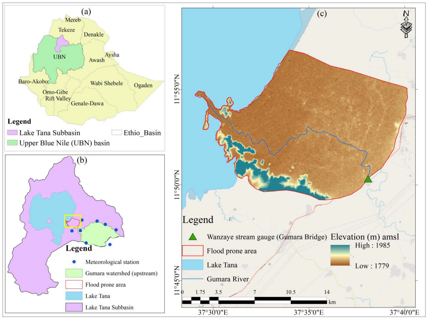
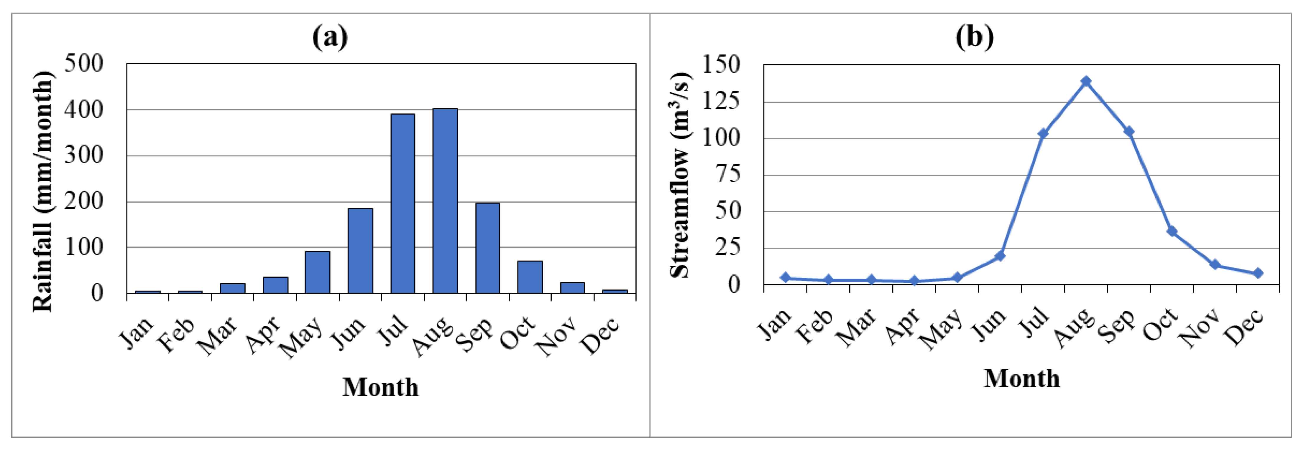
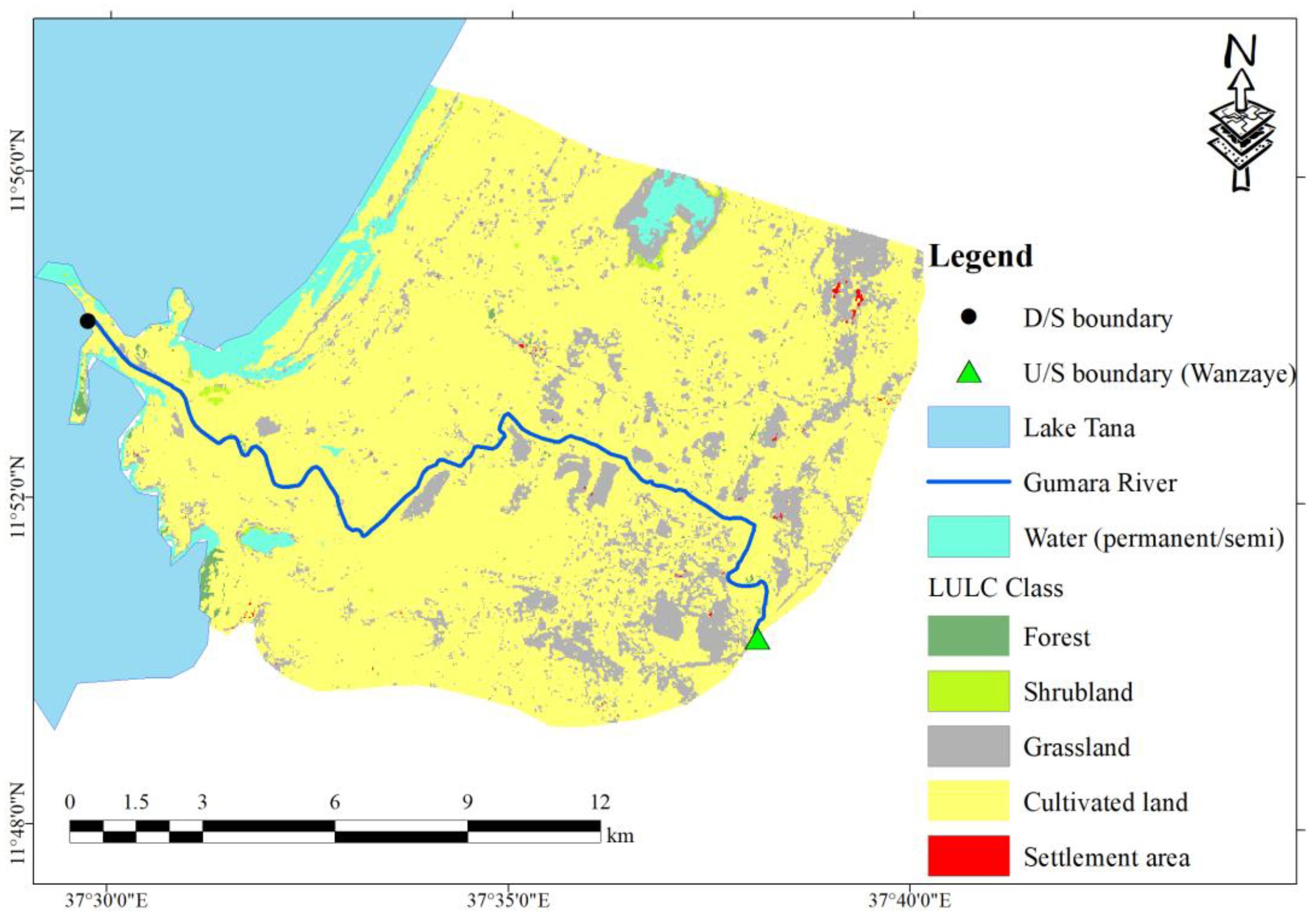
2.1. Study Area

The flood-prone area that is part of the Gumara watershed is located within the UBN Basin of Ethiopia (Figure 1). Geographically, it lies between 11°48′N–11°57′N latitude and 37°28′E–37°40′E longitude (Figure 1c). The upstream portion of the watershed, identified as the flood source area (Figure 1b), covers approximately 1256 km² and is primarily drained by the Gumara River, which originates from Guna Mountain. The flood-prone area considered in this study covers approximately 177.8 km². Topographically, the flood-prone area is relatively flat, with elevations ranging from 1779–1985 m above mean sea level (amsl). The watershed experiences a unimodal rainfall pattern, with a long rainy season spanning June–September and a mean annual rainfall of 1445 mm (Figure 2a). The streamflow of the Gumara River peaks during these months, especially in July and August (Figure 2b). Cultivated land is the dominant LULC class in both flood source and flood-prone areas [44,45]. Owing to its flat terrain and gentle slope, the flood-prone area is highly susceptible to frequent flooding caused by the overflow of the Gumara River. This vulnerability is intensified by extreme rainfall events and LULC changes in upstream areas [42,46].

2.2. Data Used

The data for SAR-based flood mapping and hydraulic flood modeling were sourced from various providers. For SAR-based flood mapping, pre- and postflood Sentinel-1A Level-1 SAR ground range detection (GRD) scenes were accessed through the European Space Agency (ESA) Copernicus Programme (https://scihub.copernicus.eu) (accessed on 20 May 2024) via the Google Earth Engine (GEE) data catalog. Time series flood inundation maps were generated via SAR data from 2017–2021, with January composite images representing preflood conditions and July–August composites representing postflood conditions each year. These images were captured in VH polarization (vertical transmit, horizontal receive), interferometric wide swath (IW) mode, and descending orbit pass mode, with a 10 m spatial resolution and a 12-day temporal interval. The 2019 flood event was selected for comparison with hydraulic flood modeling. For this year, preflood images were obtained on 11 and 23 January, whereas postflood images were acquired on 22 July, 3 August, and 27 August 2019.

To refine the flood extent maps, additional datasets were utilized. A 12.5 m resolution digital elevation model (DEM) was obtained from the Alaska Satellite Facility (ASF) (https://vertex.dac.asf.alaska.edu) (accessed on 25 May 2024) and used to generate the slope map. The derived slope map was then applied to enhance the accuracy of the flood extent map generated from the SAR data. The JRC global surface water map layer [47], which depicts spatiotemporal changes in global water bodies, was also used to mask permanent and semipermanent water bodies from flood inundation maps.

For hydraulic flood modeling, the DEM obtained from the ASF was used as a primary input. Sample river cross-sections of the Gumara River (downstream), along with elevation data for high and low ground, were collected through field surveys and Google Earth images for terrain modification. The LULC map for 2019 was sourced from Belay et al. [44].

The observed daily time series discharge data (1981–2019) for the Gumara River at the Wanzaye gauging station were collected from the Ministry of Water and Energy (MoWE) of Ethiopia. These data served as the upstream boundary conditions for simulating the observed flood event. Additionally, daily observed rainfall data (1981–2019) were obtained from the Ethiopian Meteorological Institute (EMI). Inflow hydrographs of the upstream Gumara watershed for various return periods (5, 10, 25, 50, and 100 years), as well as for extreme conditions during the historical (1981–2005), near-future (2031–2055), and far-future (2056–2080) periods, were sourced from Belay et al. [48] and used as boundary conditions. In Belay et al. [48], these inflow hydrographs for the upstream watershed were generated by counting future extreme rainfall and projected LULC data for the years 2035 and 2065.

Ground control points (GCPs) for flooded and nonflooded areas were collected to validate the hydraulic flood model. These GCPs were generated via Sentinel-2 imagery and field investigations in the most flood-affected areas. A Sentinel-2 Level-2A surface reflectance (SR) image from August 30, 2019, with a 10 m spatial resolution, was accessed via the GEE from the ESA for this purpose. This image was selected because it has minimal cloud cover, allowing for more accurate GCP generation in combination with information from field investigations.

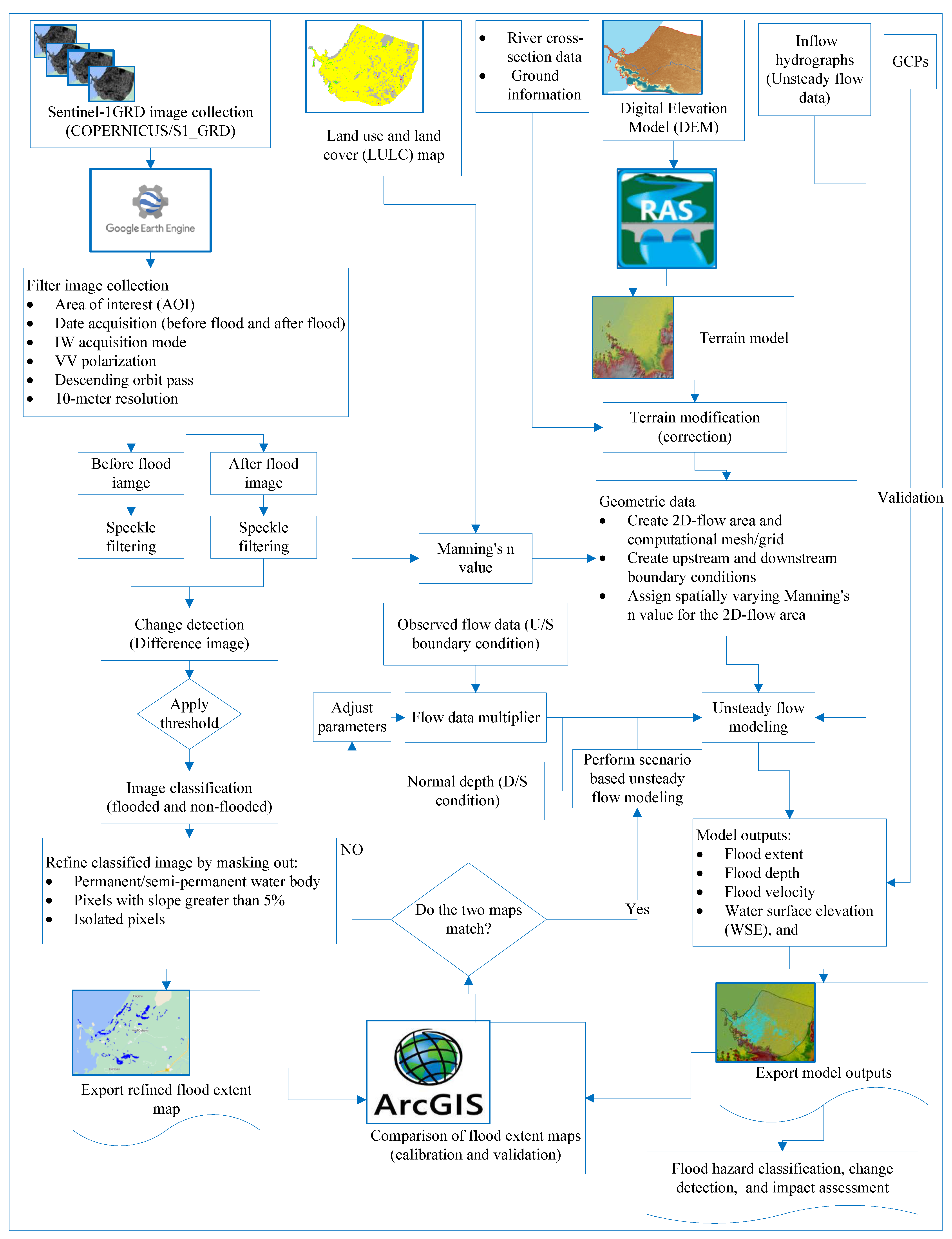
2.3. Methodological Framework of This Study

In this study, SAR-based flood inundation maps were generated via Sentinel-1 SAR images within the Google Earth Engine (GEE) environment, while hydraulic flood modeling was conducted via HEC-RAS 2D. Figure 3 illustrates the overall methodological framework of this study. Details of the methods used are provided in the subsequent sections.

2.4. SAR-Based Flood Inundation Mapping

SAR-based flood inundation mapping was conducted within the GEE environment. The process involved several steps: data acquisition and filtering of image collections, preprocessing, change detection, and refining and exporting flood extent maps.

2.4.1. Importing and Filtering of SAR Image Collection

Sentinel-1 SAR images before the flood (preflood) and during the flood (postflood) were acquired in GRD format via the GEE data catalog. To select a subset of SAR images, the image collection was filtered on the basis of various metadata properties, such as the filter bounds, date of acquisition, instrument mode, transmitter and receiver polarizations, orbit pass properties, and resolution. The shapefile of the flood-prone area was imported into the GEE environment as an asset and used as a filter bound. A composite of SAR images acquired for 11 and 23 January 2019 was used as the preflood image since this period was the dry season in the study area. Images acquired on 22 July, 3 August, and 27 August 2019 (during the flood) were used to map the floods that occurred on those dates. The images were acquired in IW instrument mode with VH polarization, a descending orbit pass, and a spatial resolution of 10 × 10 m. The IW mode was selected because it is the primary acquisition mode for land surfaces.

A similar procedure was followed for importing and filtering SAR images from 2017–2021. Time series inundation maps were prepared via composites of January images as preflood conditions and composites of July–August images as postflood conditions instead of focusing on specific flood events. This approach aimed to map flood frequency in the region over a five-year period.

2.4.2. Preprocessing

Sentinel-1 SAR images often suffer from various types of errors and noise, such as geometric and radiometric distortions, thermal noise, and speckle [49,50]. Therefore, these noises need to be corrected through preprocessing steps before the data can be used for flood inundation mapping. The GEE platform has already applied the following preprocessing steps: (i) Orbit file correction is used to update the metadata of the orbit. (ii) Border noise removal eliminates invalid data (e.g., low-intensity noise) at the edges of the scene. (iii) Thermal noise removal eliminates additive noise, such as discontinuities between subswaths in SAR scenes with multiswath acquisitions. (iv) Radiometric calibration is used to convert digital pixel values to calibrated SAR backscatter coefficients (σ°) on the basis of sensor calibration parameters. (v) Terrain correction is used to remove geometric distortion in SAR images. (vi) σ° is converted to decibels (dB) and a logarithmic transformation of (10 × log10σ°) is used to convert the unitless σ° to dB.

Sentinel-1 Level-1 GRD images, which have already undergone automated preprocessing steps, were used for this study. Despite these preprocessing steps, the images still contained speckle noise, which appeared as granular noise caused by the coherent nature of SAR imaging. To reduce the effects of speckle noise, speckle filtering or smoothing was applied to both preflood and postflood images. Specifically, a refined Lee speckle filter [49] with a window size of 3 × 3 was employed within the GEE environment.

2.4.3. Change Detection and Thresholding

A change detection approach was employed to map the flood extent. This method involves dividing the postflood image by the preflood image to generate a difference image, which is then classified into a binary image representing flooded and nonflooded areas. To create the binary raster, a threshold value was applied to the difference image. The selection of an appropriate threshold value depends on various factors, including the type of flood, the characteristics of the SAR images, and the conditions of the surrounding area. The optimal threshold was determined through visual inspection and frequency distribution analysis (histogram thresholding) [28,30]. Since the frequency distributions of flooded and nonflooded pixels follow a bimodal pattern with two distinct peaks, the threshold was set at the transition zone (valley) between the two peaks.

Furthermore, the percentage area of flooded pixels was also computed to analyze the sensitivity of the flood extent to different threshold values, which could guide the determination of the optimal threshold value. Following these methods, the optimal threshold was determined for separating flooded pixels from nonflooded pixels.

2.4.4. Refining and Exporting Flood Extent Maps

To increase the accuracy of the flood extent map generated through the change detection approach, additional datasets were used to refine the results by eliminating overestimated flood areas. Among these, the JRC global surface water mapping layer dataset was used to exclude areas covered by permanent and semipermanent water, applying a seasonality threshold greater than 10 months per year. This dataset effectively masked water in wetlands and along lakes.

A slope layer derived from a 12 m DEM was also used to exclude false positives in the flood mapping process. This is because steep areas are generally less prone to flooding, and any SAR-detected flooding in such regions is likely to be a false positive. For this study, flooded pixels in areas with slopes greater than 5% were masked out, following recommendations from previous studies [51,52], to improve the accuracy of flood detection.

In SAR-based flood mapping, wet soil and certain vegetation (e.g., rice fields) may exhibit low backscatter similar to floodwater, potentially leading to misclassification (false positives) [53,54]. To address this issue, the connectivity of flooded pixels was assessed, and isolated flood pixels were removed to minimize noise and enhance the accuracy of the final flood map. Specifically, pixel connectivity was first analyzed via the GEE function recommended by UN-SPIDER [51]. Then, the pixels connected to eight or fewer neighbors were removed, as they were more likely to be false positives.

To compute the areal extent of the flood mapping output, the refined raster binary layer (flooded and nonflooded) prepared in the GEE was exported, and final processing was performed in ArcGIS 10.4. The areal extent of the flooded area in m² was computed by summing the area of each flooded pixel. Additionally, to estimate the impact of flooding on cultivated land, spatial analysis and spatial statistics tools were used in the ARC-GIS environment for overlay analysis.

2.5. Hydraulic Flood Modeling

Hydraulic flood modeling was conducted via the HEC-RAS model (version-6.5). This model has the ability to perform 2D unsteady flow modeling on the basis of full shallow water (SW) and diffusion wave (DW) equations [34]. These equations can perform detailed 2D channel and floodplain mapping with high flexibility [55,56]. From these equations, 2D DW equations were chosen for this study, as these equations can perform unsteady flow modeling more quickly with high stability [39].

The 2D DW equation solver in HEC-RAS uses an implicit finite volume algorithm, as this algorithm provides improved stability and allows for performing flow simulations for larger computational time steps than finite difference and finite element methods [57]. The 2D DWE is derived from mass conservation and momentum equations, as described below:

Mass conservation equation: In 2D flood modeling, the mass conservation equation (also known as the continuity equation) governs how water depth changes over time and how water is transported within the floodplain [56,58]. This ensures that water is conserved in the model by considering both changes in water depth and the velocity field across the domain. The equation is expressed as:

$${\displaystyle \frac{\partial h}{\partial t}}+{\displaystyle \frac{\partial \left(hu\right)}{\partial x}}+{\displaystyle \frac{\partial \left(hv\right)}{\partial y}}=0$$

(1)

where $h$ represents the depth of the water, $u$ represents the velocity of the water along the $x$-axis, $v$ represents the velocity of the water along the $y$-axis, $t$ represents time, and $x$ and $y$ represent location information. In Equation (1), the first term represents (${\displaystyle \frac{\partial h}{\partial t}})$, the rate of change in water depth over time, whereas the second (${\displaystyle \frac{\partial \left(hu\right)}{\partial x}})$ and third (${\displaystyle \frac{\partial \left(hv\right)}{\partial y}})$ terms represent the fluxes of water (the rates of flow of water) in the x and y directions, respectively.

Momentum equations: In 2D flood modeling, the momentum equation describes the movement of water on the basis of the forces acting on it [56,58]. In the 2D DW equation, the momentum equations are simplified by neglecting the inertia (acceleration) terms of the full dynamic equation, assuming that the flow is governed primarily by gravity and friction [56]. The equation is expressed as follows:

Along the $x$-axis:

$$S_{0x}-S_{fx}-{\displaystyle \frac{\partial h}{\partial x}}=0$$

(2)

Along the $y$-axis:

$$S_{0y}-S_{fy}-{\displaystyle \frac{\partial h}{\partial y}}=0$$

(3)

where $S_{0x}$ and $S_{0y}$ are bed slopes in the $x$ and $y$ directions, respectively. ${\displaystyle \frac{\partial h}{\partial x}}$ and ${\displaystyle \frac{\partial h}{\partial y}}$ represent the slopes of the water surface in the x and y directions, respectively. $S_{fx}$ and $S_{fy}$ are the friction slopes in the $x$ and $y$ directions, respectively. The bed slope term expressed in the momentum equations can be computed from the underlying elevation data (DEM), whereas the friction slope terms are determined via Manning’s equation, which relates friction (flow resistance) to depth and velocity.

$$S_{fx}={\displaystyle \frac{n^{2}u\sqrt{u^2+v^2}}{h^{\raisebox{1ex}{$4$}\!\left/ \!\raisebox{-1ex}{$3$}\right.}}}$$

(4)

$$S_{fx}={\displaystyle \frac{n^{2}v\sqrt{u^2+v^2}}{h^{\raisebox{1ex}{$4$}\!\left/ \!\raisebox{-1ex}{$3$}\right.}}}$$

(5)

where $n$ is Manning’s roughness coefficient; $u$ and $v$ are the velocity components in the $x$ and $y$ directions, respectively; $h$ is the water depth; and $u^2+v^2$ represents the total velocity magnitude.

The 2D flow model in HEC-RAS was set up using a 2D flow area to represent the floodplain. For this purpose, the RAS mapper of the HEC-RAS model was used to import terrain data and other features, create and refine geometric data, and visualize the HEC-RAS simulation results. Overall, hydraulic flood modeling involves terrain preprocessing, creating a 2D flow area and computational mesh, defining boundary conditions, assigning Manning’s roughness value, and conducting unsteady flow analysis followed by output mapping. Details of these procedures are provided in the following section.

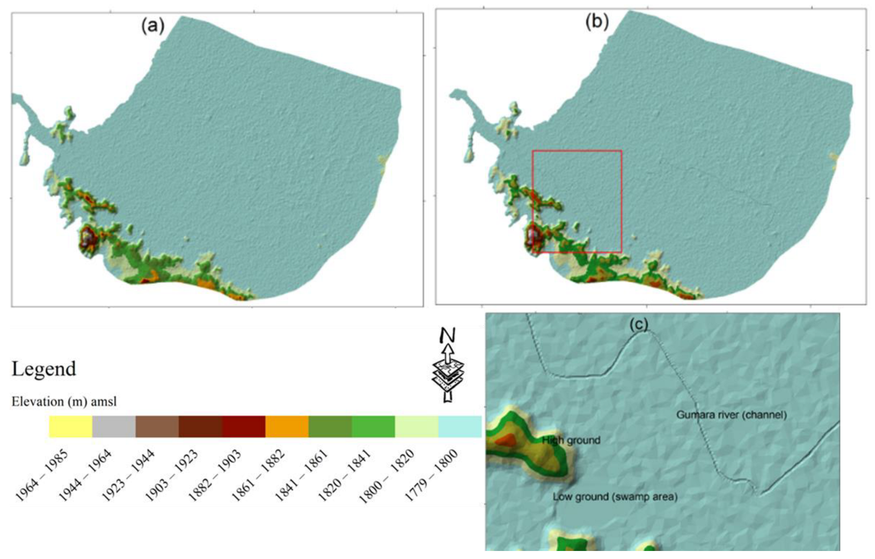
2.5.1. Terrain Preprocessing

In the HEC-RAS model, terrain data are essential for determining the geometric and hydraulic properties of 2D computational meshes. In this study, a 12.5 m resolution DEM was used to develop the terrain model. The vertical accuracy of this DEM, expressed in terms of the root mean square error (RMSE), was found to be approximately 3.5 m. However, this DEM does not include the actual terrain beneath the water surface in the river, diversion channels, or other low-lying areas. To address these gaps, a total of 17 river cross-sections, the hydraulic properties of the diversion channel, and elevation data for low- and high-elevation areas were incorporated. These data were obtained from Google Earth by extracting elevation profiles (as Supplementary Data) and from field surveys. The collected information was then used to modify and improve the original terrain model. Figure 4 below shows the original and modified terrain models in the triangulated irregular network (TIN) format. The station and elevation data for the cross-sections, along with a comparison of elevation data from the DEM and ground observations, are provided in the Supplementary Materials Tables S1 and S2, Figure S1 and S2.

2.5.2. Two-Dimensional Flow Area and Computational Mesh

In HEC-RAS, flood-prone areas can be delineated via background web-based satellite imagery, terrain models, and various map layers to accurately define floodplains [34]. For this study, a 2D flow area was created for the downstream section of the Gumara River, extending from the Gumara Bridge at Wanzaye to the shores of Lake Tana. This area includes floodplains frequently affected by riverine flooding, following previous studies [43,59] conducted in the downstream Gumara River watershed. During the delineation of the 2D flood area, high-elevation areas that could obstruct floodwater flow were primarily used as boundaries (Supplementary Materials Figure S4).

Following the creation of the 2D flow area, the next step was to generate the 2D computational grid/mesh. The computational grids consist of various shapes, including triangles, rectangles, squares, and polygons with up to eight sides. Each grid cell within the computational mesh includes a cell center, cell faces, and cell face points. The cell center is the computational point where the water surface elevation and depth are calculated. The cell faces are typically straight or multipoint lines that define the boundaries of the cell center, whereas the cell face points are the endpoints of these cell faces. The cell faces pointing at the outer boundary of the 2D flow area are used to connect the 2D flow area to other flow elements and boundary conditions.

In this study, the computational mesh was created in the HEC-RAS geometric data editor by specifying grid spacing in terms of DX and DY. Following Casulli [60], a relatively coarser computational grid–cell spacing than the horizontal resolution of the underlying terrain (12.5 m) was used to improve the computation time. To determine the optimal grid–cell spacing, the model stability was evaluated via grid spacing values of 40 m, 50 m, and 60 m following studies by Costabile et al. [39] and Psomiadis et al. [10]. Stability was assessed on the basis of the convergence of results and computational efficiency. The model was found to be stable with a grid–cell spacing of 50 m (DX = 50 m and DY = 50 m), which provided a good balance between accuracy and computation time. This resulted in the creation of 70,740 grid cells, with an average area of 2512.64 m².

2.5.3. Boundary Conditions and Manning’s Roughness Coefficient (n Value)

The upstream boundary condition, which represents the point where the flow enters the 2D flow area, was established at the Gumara Bridge, which is located at the Wanzaye stream gauging station (Figure 5). The downstream boundary condition, where the flow exits, was set at the inlet of the Gumara River into Lake Tana.

In HEC-RAS 2D flood modeling, Manning’s roughness coefficient (n) is a critical parameter influencing flow resistance and model accuracy. The latest version of HEC-RAS (6.5) supports importing LULC maps from various sources, facilitating the precise estimation of n values. In this study, the 2019 LULC map (Figure 5) was used to derive initial estimates of spatially varying n values. Using these LULC data, Manning’s n values corresponding to different LULC classes were initially assigned on the basis of the recommendations of Chow [61]. Following the initial estimation of the n values, the optimal values were determined through model calibration.

2.5.4. Unsteady Flow Analysis

Unsteady flow modeling in HEC-RAS 2D requires unsteady flow data for upstream and downstream boundary conditions. In this study, time series flow data from the Gumara River (21 July–31 August 2019) were used as the upstream boundary conditions (Supplementary Materials Figure S3). An average bed slope of 0.0012 was used as the downstream boundary condition for the Gumara River, corresponding to a uniform (gradually varied) flow regime. Additionally, an initial water surface elevation (WSE) of 1785.5 m amsl was set to account for the water present in the river channel and permanent/semipermanent water bodies at the start of the simulation. Grid cells with elevations above this WSE were considered dry, whereas those below it were considered wet, with initial depths varying on the basis of terrain conditions.

In HEC-RAS 2D unsteady flood modeling, selecting an appropriate computational interval (Δt) is crucial for achieving accurate model outputs, including depth, water surface elevation, and velocity. It is also essential for ensuring model stability during flood simulation. Factors such as the mesh cell size and flow velocity influence the determination of ∆t. Among the various methods available, the Courant–Friedrichs–Lewy (CFL) condition [62] was employed in this study to determine $∆t$. In this method, to ensure model stability, the CFL condition is given as:

$$CFL={\displaystyle \frac{v∆t}{∆x}}\le 1;$$

(6)

Solving for $∆t$ from Equation (6) yields:

$$∆t=CFL{\displaystyle \frac{∆x}{v}}$$

(7)

where $\Delta t$ is the computation interval (s), $\mathsf{\Delta }x$ is the mesh/grid cell size (m), $v$ is the flood water velocity (m/s), and CFL is the Courant–Friedrichs–Lewy number, which is simply the Courant number.

2.5.5. Model Sensitivity Analysis

Sensitivity analysis is an essential step in evaluating how variations in input parameters influence model outputs [63]. It is typically measured as the positive or negative percentage change in model output relative to a reference scenario. In this study, the sensitivities of flood depth and inundation area were analyzed with respect to changes in Manning’s roughness coefficient ($n$). The analysis was performed by systematically increasing/decreasing the reference Manning’s $n$ from −25% to 25% at 5% intervals following a similar procedure to the one provided in Ghimire et al. [64]. The resulting changes in flood depth and inundation area were computed relative to the results obtained via the baseline Manning’s $n$ value. The baseline Manning’s $n$ values were determined on the basis of the average of the upper and lower bounds provided for different land use and river channel types by Chow [61]. The percentage changes in flood depth and inundation area were calculated as follows:

$$Change in depth\left(\mathrm{\%}\right)={\displaystyle \frac{{Depth}_{new}-{Depth}_{baseline}}{{Depth}_{baseline}}}$$

(8)

$$Change in area\left(\mathrm{\%}\right)={\displaystyle \frac{{Area}_{new}-{Area}_{baseline}}{A_{baseline}}}$$

(9)

where ${Depth}_{new}$ and ${Area}_{new}$ represent the flood depth and inundation area computed via different Manning’s $n$ values, respectively, whereas ${Depth}_{baseline}$ and ${Area}_{baseline}$ represent the flood depth and inundation area computed via the baseline Manning’s $n$ value. In this study, model sensitivity analysis was conducted for flood events that occurred on 5 August 2019.

2.5.6. Model Calibration

In HEC-RAS 2D flood modeling, observed hydraulic data, including flood depth, water surface elevation, and flow velocity, are essential for calibration [64,65]. However, in the absence of such data, several studies have recommended the use of flood inundation maps derived from remote sensing imagery, particularly from optical sensors and SAR sensors [37,66,67]. Among these, SAR-derived flood extent maps are widely used for calibrating HEC-RAS model parameters [10,11]. For this study, since observed hydraulic data were unavailable, the HEC-RAS model parameter, specifically Manning’s roughness coefficient (n), was calibrated via SAR-derived flood extent maps from 22 July, 3 August, and 27 August 2019.

The calibration procedure involved several steps. First, initial Manning’s n values were assigned for different land use types and river channels on the basis of published references. In this study, the average of the upper and lower bounds of Manning’s roughness values for each land use type and river channel, as provided in Chow [61], was assigned as the initial or baseline roughness value. Using these initially assigned n values, a flood simulation was performed, and the resulting flood map was compared with the SAR-derived flood map. The match between the simulated and SAR-derived flood maps was evaluated through visual inspection and the quantitative metrics described in Section 2.5.7.

Following the initial comparison, the Manning’s n value for each land use type and the river channel was gradually adjusted. The adjustment of Manning’s n during calibration ranged from −25% to +25%, with intervals of 5%. The calibration was conducted manually by adjusting the roughness values of different land use types simultaneously. The optimal roughness values for each land use type were determined after 33 trial flood simulations were conducted (11 for each flood event). For this purpose, performance metrics were computed for each trial simulation of flood events (e.g., for the 22 July 2019 flood event). The Manning’s roughness values that resulted in the highest performance scores were selected. The same procedure was followed for the flood events of 3 August and 27 August 2019. Finally, the calibrated Manning’s n values were determined by averaging the optimal values obtained from the three events.

In addition to calibrating Manning’s n values, a min-flow multiplier was applied to flow values lower than the mean flow, ensuring better agreement between the HEC-RAS model-simulated and SAR-based inundation maps. This approach involves computing the mean flow of the time series data or flow hydrograph and applying a multiplier only to flows below the mean while keeping higher flows unchanged. This is important for improving the numerical stability of the model and maintaining computational accuracy [56]. For this purpose, min-flow multipliers ranging from 1.01 to 1.05 were tested with a 0.01 interval, and the best-performing value was selected to make slight min-flow adjustments.

2.5.7. Model Performance Evaluation

The performance of the HEC-RAS model during calibration was evaluated via performance metrics such as the $F1$ score, overall accuracy ($OA$), and kappa coefficient ($K$). The $F1$ score (Equation (10)) quantifies the model’s predictive ability, ranging from 0 to 1, with values approaching 1 indicating better performance in predicting flood extent. $OA$ (Equation (11)) measures the agreement between HEC-RAS-modeled flood maps and SAR-derived flood maps, where values closer to 1 signify higher accuracy. $K$ (Equation (12)) evaluates the level of agreement beyond chance between modeled and observed flooded pixels, ranging from −1 to 1, with values near 1 indicating strong agreement. These metrics were selected for their broad applicability in comparing model-simulated and SAR-derived inundation maps [37,55,67] and their ability to provide a comprehensive performance evaluation from multiple perspectives [68,69].

$$F-\mathrm{s}\mathrm{c}\mathrm{o}\mathrm{r}\mathrm{e}={\displaystyle \frac{TP}{TP+FP+FN}}$$

(10)

$$OA (\%)={\displaystyle \frac{TP+TN}{TP+FN+FP+TN}}$$

(11)

$$K={\displaystyle \frac{P_o-P_e}{1-P_e}}$$

(12)

$$P_o={\displaystyle \frac{TP+TN}{T}}$$

(13)

$$P_e={\displaystyle \frac{\left(TP+FP\right)*\left(TP+FN\right)+\left(TN+FP\right)*(TN+FN)}{T^2}}$$

(14)

where $TP$ (true positive) represents correctly predicted flooded pixels, TN (true negative) represents correctly predicted nonflooded pixels, FP (false positive) represents pixels incorrectly predicted as flooded, and FN (false negative) represents actual flooded pixels missed by the model. For the kappa coefficient ($K)$, $P_o$ is the observed agreement, $P_e$ is the expected agreement, and T is the total number of pixels in the flood map, which is (TP + FN + FP + TN).

2.5.8. Model Validation

To further validate the HEC-RAS model, GCPs for flooded and nonflooded areas were collected for the study area. These GCPs were obtained on the basis of Sentinel-2 multispectral optical imagery and field visit information from the areas most frequently affected by floods. Sentinel-2 imagery was selected because it is widely used in flood monitoring and the generation of validation points [69,70,71]. Additionally, floodwater can be easily detected because of its multispectral bands [70]. For this study, the Sentinel-2 image from August 30, 2019 was accessed via the GEE and used for collecting the GCPs. Using this approach, 150 flooded and 150 nonflooded GCPs were collected and compared with the flood extent map of the HEC-RAS model.

Model performance was evaluated via key performance metrics, including $OA$, $K$, producer accuracy ($PA$), user accuracy ($UA$), omission error ($100-PA$), and commission error ($100-UA$). These metrics were chosen for their broad applicability in flood-related studies, as they evaluate performance from both the producer’s and the user’s perspectives [69,70,71].

2.5.9. Flood Hazard Mapping

Flood hazard classification is important for assessing the potential impacts of flooding on different areas and plays a crucial role in supporting flood risk management strategies and enhancing emergency preparedness efforts [66]. It involves categorizing areas according to key flood characteristics such as flood depth and velocity. In this context, several guidelines have been developed in different countries to classify flood hazards. The depth–velocity product (DVP) method of flood hazard classification was employed for this study on the basis of the UK Department for Environment, Food, and Rural Affairs (DEFRA) guidelines [72] presented in

Table 1. Depth–velocity product (DVP) method for flood hazard classification [72].

Hazard Class	DVP (m2/s) Hazard Rating
Low (H1)	DVP < 0.75
Moderate (H2)	0.75 ≤ DVP < 1.25
Significant (H3)	1.25 ≤ DVP < 2.0
Extreme (H4)	DVP ≥ 2.5

.

2.5.10. Flood Inundation Mapping for Different Return Periods and Under Changing LULC and Climate Conditions

Flood inundation mapping for various return periods (5, 10, 25, 50, and 100 years) was conducted via the calibrated HEC-RAS model. In this analysis, inflow hydrographs (Figure 6a) computed via HEC-HMS from annual maximum 1-day rainfall data (1981–2019) were applied as upstream boundary conditions. These hydrographs were obtained from our recent work [48].

To examine the impacts of LULC and climate changes in the upstream Gumara wa-tershed on downstream flood inundation, the HEC-RAS model was further run via inflow hydrographs representing extreme conditions (Figure 6b) sourced from our recent work [48]. These hydrographs, derived from HEC-HMS simulations, were based on the ensemble means of four CMIP6 models. The simulations spanned historical (1981–2005), near-future (2031–2055), and far-future (2056–2080) periods under the high-emission scenario SSP5-8.5 [48]. In this analysis, historical LULC maps for 2000 and 2010 were used to represent baseline conditions, whereas projected LULC maps for 2035 and 2065 represented near-future and far-future scenarios, respectively. The integration of LULC and climate scenarios enabled the generation of inflow hydrographs that captured the combined impacts of these changes on flood inundation. This integrated approach provides valuable insights for flood management and planning in the Gumara watershed. Detailed methodologies for inflow hydrograph simulations across scenarios are provided in Belay et al. [48]. The relative change in flood inundation extent between the historical and future periods was computed via the following equation:

$$Relative Change\left(\mathrm{\%}\right)={\displaystyle \frac{A_{future}-A_{historical}}{A_{historical}}}\times 100$$

(15)

where $A_{historical}$ and $A_{future}$ represent the total flood area (km²) during the historical and future periods, respectively.

3. Results

3.1. SAR-Based Flood Inundation Maps

As described in the methods section, SAR-based flood mapping was conducted via the GEE cloud-based platform following a change detection approach. The following Section 3.1.1, Section 3.1.2, Section 3.1.3 and Section 3.1.4 detail the characteristics of preflood and postflood images, the results of change detection and thresholding, and the refined flood inundation map generated through this method.

3.1.1. Pre- and Postflood SAR Images

Flood inundation mapping was conducted via SAR images acquired before and after the flood, as detailed in the methods section. The preflood images were acquired before the flood event and served as a reference, whereas the postflood images were acquired during or after the flood event and used to map areas inundated by floodwater. A composite of SAR images from 11 and 23 January 2019 was used to capture the preflood conditions of the area (Figure 7a). These images were selected because January is typically a dry month in the study area. SAR images for 22 July, 3 August, and 27 August 2019 (Figure 7b–d, respectively) were used to delineate flood inundation on those dates. These specific images were chosen on the basis of the availability of SAR data for the given dates and to analyze the initiation, progression, and recession of floodwaters in the study area. All the images were processed through automated preprocessing steps in the GEE environment, and speckle filtering was applied via the Lee filter [49] to reduce noise (speckles) in the images.

In the SAR images (Figure 7b–d), indicated with a red rectangle, the flooded areas appear dark due to low backscatter (σ⁰) caused by specular reflection. In specular reflection, radar waves hitting smooth surfaces, such as water, are reflected away from the SAR sensor, resulting in few or no waves returning back to the sensor [19,25]. This causes flooded areas to appear dark in SAR images. Conversely, nonflooded areas (such as dry land surfaces or vegetation covers) appear brighter in SAR images because of higher backscatter values, as these areas reflect more radar waves back to the sensor [73]. On the other hand, permanent/semipermanent water bodies stored in wetlands and lake shores (indicated in the blue rectangle) remained unchanged before and after the flood (Figure 7a–d).

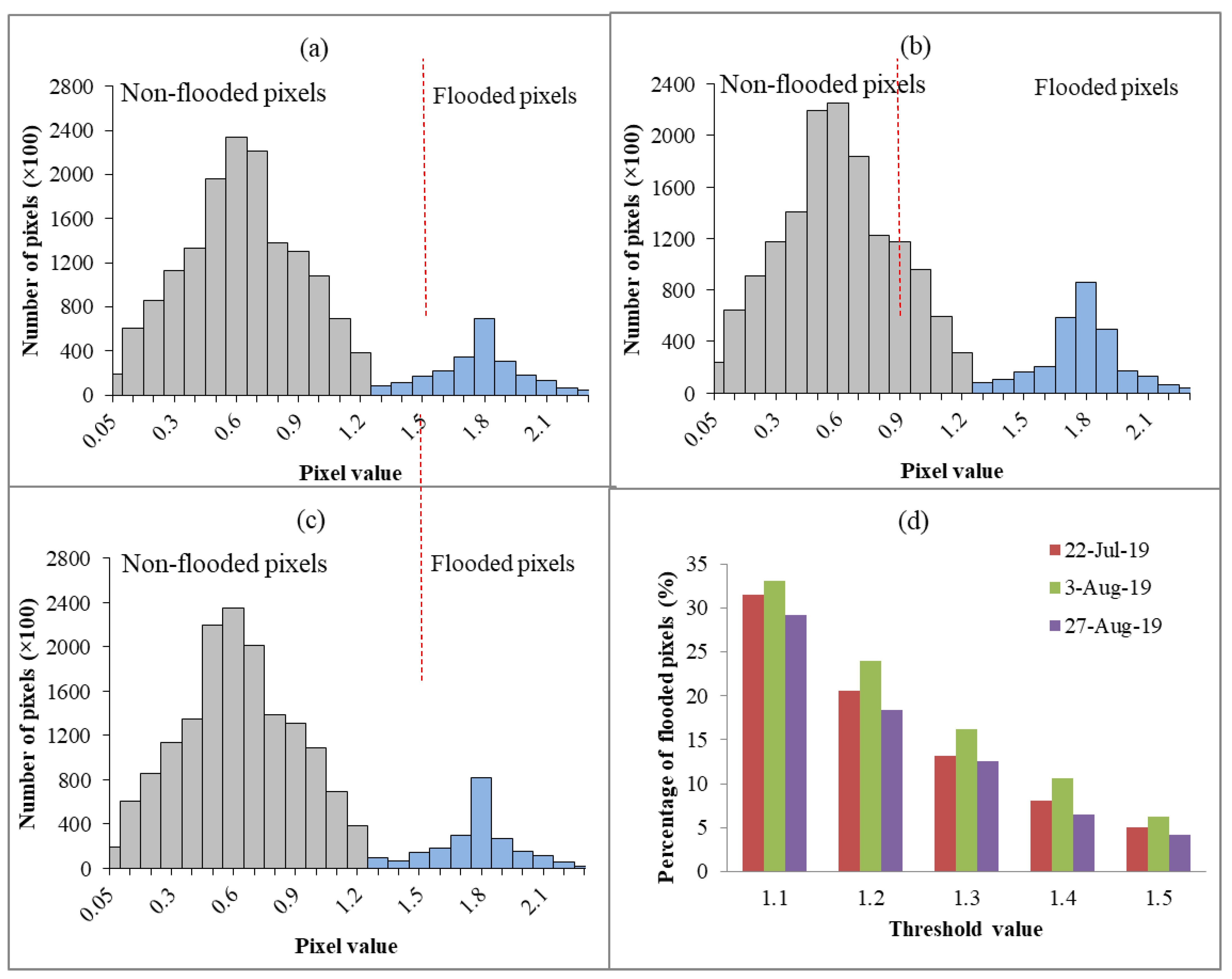
3.1.2. Change Detection and Thresholding

SAR-based flood inundation maps for the study area were generated by classifying the difference image into binary categories: flooded and nonflooded areas. Figure 8a–c show the pixel values of the difference image for the three flood events of 2019. In these figures, darker pixels indicate flooded areas with higher change magnitudes, whereas brighter pixels represent nonflooded areas with lower pixel values.

Figure 9a–c illustrate the frequency distributions for three flood events in 2019, revealing a bimodal pattern with two distinct peaks. The transition zone between flooded and nonflooded pixels lies between 1.2 and 1.5. Among these, the threshold values of 1.30 and 1.40 were identified as optimal, corresponding to the lowest frequency (i.e., the valley) in the bimodal distribution. Specifically, a threshold of 1.30 was selected for the flood events on 22 July and 3 August 2019, whereas a threshold of 1.40 was chosen for the 27 August 2019 flood. Additionally, Figure 9d illustrates the percentage of flooded pixels for each event across threshold values from 1.10–1.50, revealing a decreasing trend in flooded pixels as the threshold increases.

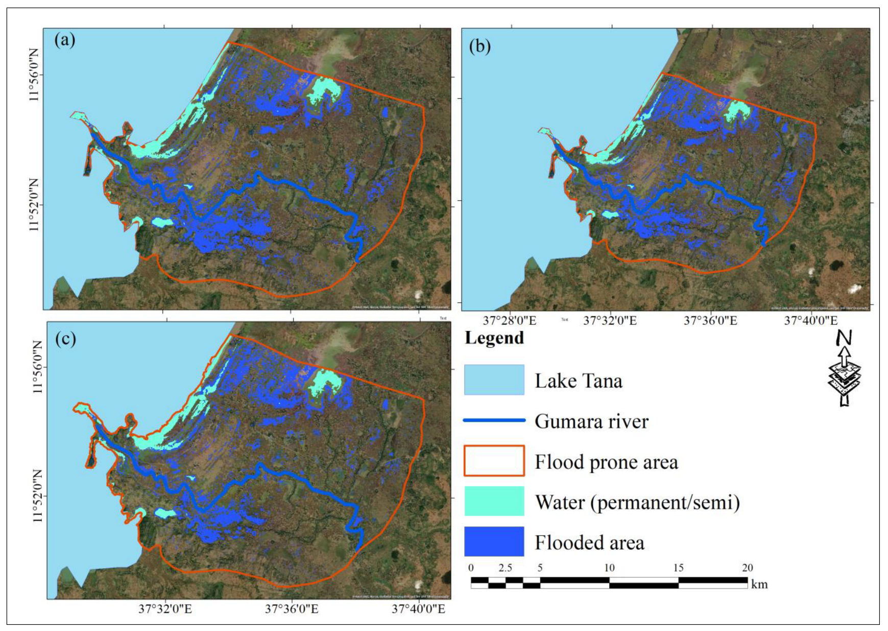
3.1.3. SAR-Based Flood Inundation Maps for 2019

To further refine the flood extent map generated via the change detection and thresholding approach, permanent/semipermanent water bodies, areas with slopes greater than 5%, and isolated or misclassified pixels were masked during the classification process, as detailed in the methods section. Figure 10 shows the refined flood inundation maps from July and August 2019. As illustrated in Figure 10a, flood inundation on 22 July 2019, was predominantly concentrated in the northern and southern parts of the flood-prone area, with a few isolated flood spots scattered across other regions. By 3 August 2019, as shown in Figure 10b, the flood had significantly progressed north and south. By 27 August 2019, as depicted in Figure 10c, the floodwaters had receded, especially in the southern and northern regions, with the remaining inundation confined primarily to depressions and wetlands.

For the study area, the flooded area was computed via ARC-GIS. The results revealed that the inundated areas were 23.46 km², 28.86 km², and 22.26 km² on the three dates. This shows the initiation, expansion, and recession of the flood in the study area across these dates. In the study area, the distribution of floodwaters was influenced mainly by terrain conditions. The floodwater was concentrated along the course of the Gumara River, in low-lying areas (depressions), and in wetlands along the shoreline of Lake Tana, where the topography is nearly flat. Among the total flood-inundated area, cultivated land accounted for more than 97%, while the remaining area was accounted for by other land use classes.

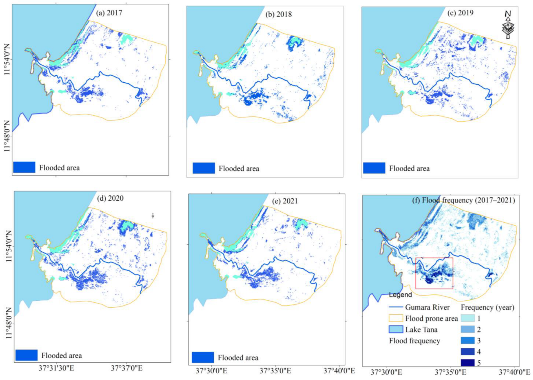
3.1.4. SAR-Based Flood Frequency Mapping

To assess the flooding conditions in the study area, the flood frequency was analyzed via time series flood maps derived from Sentinel-1 SAR images over a five-year period (2017–2021). For each year, composite SAR images from January were used to represent preflood conditions, whereas composite images from July and August were used to capture postflood conditions. The resulting flood inundation maps for each year were then combined to determine the flood frequency. Figure 11a–e present the time series flood maps from 2017–2021, whereas Figure 11f displays the flood frequency over this period. As shown in the maps, the flood frequency is highest near the meandering section of the Gumara River, highlighted within the red rectangle.

Table 2. Optimal threshold values and SAR-derived flood inundation areas from 2017–2021.

Year	Optimal Threshold Value	Flood Inundation Area (km2)
2017	1.30	14.09
2018	1.25	11.22
2019	1.30	15.00
2020	1.34	21.15
2021	1.30	16.41
Average	1.32	15.57

also provides the optimal threshold values used to distinguish flooded and nonflooded pixels, along with the corresponding flood extent for each year. According to the results, the highest flood inundation occurred in 2020, whereas the lowest flood inundation was observed in 2017.

3.2. Hydraulic Flood Modeling

The 2D unsteady flood simulation was conducted via the HEC-RAS model along a 26.56 km reach of the Gumara River, from Gumara Bridge at Wanzaye (upstream) to Lake Tana (downstream), encompassing the surrounding floodplain areas. To ensure model stability, a Courant–Friedrichs–Lew (CFL) value of 0.7 was employed, as recommended for flood simulations over flat floodplains [34]. On the basis of the CFL value, a floodwater velocity of 1.2 m/s (typical for flat floodplain areas), and a mesh size of 50 m, the computational time step was set to 30 s.

The simulation utilized time series streamflow data from 20 July to 31 August 2019 as the upstream boundary condition. On the basis of the simulation results, the flood event on 5 August 2019 was selected for model sensitivity analysis to change the HEC-RAS model parameters. The flood events on 22 July, 3 August, and 27 August 2019 were chosen for model calibration because they aligned with the Sentinel-1 SAR data. The flood event on 30 August 2019 was selected for validation because of the availability of a less cloudy Sentinel-2 image on this date, which was used to generate validation points for flooded and nonflooded areas.

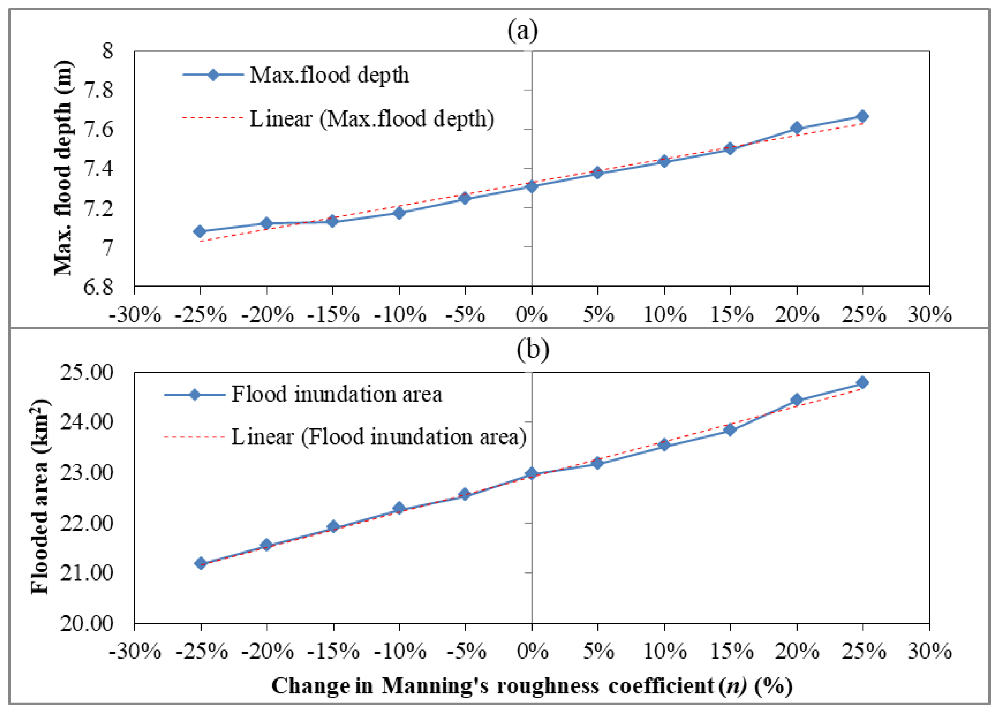
3.2.1. Sensitivity Analysis

Figure 12a presents the sensitivity of flood depth to variations in Manning’s n within a range of −25% to +25%. The results indicate a gradual increase in flood depth with increasing Manning’s n values. This occurs because higher roughness increases resistance to flow, slowing the floodwater and causing greater accumulation (higher inundation depth) in the floodplain.

Similarly, Figure 12b illustrates the sensitivity of the flood inundation area to changes in Manning’s n values. As with flood depth, the inundation area also expands with increasing roughness due to the increased frictional resistance, which slows floodwater movement, leading to greater water ponding and a broader flood extent. These findings align with previous studies that have demonstrated the sensitivity of flood depth and inundation area to changes in Manning’s roughness n values [64,74]. Figure S4a–c in the Supplementary Materials also show the variation in flood inundation depth for −25%, baseline, and +25% changes in Manning’s roughness n values, respectively.

The percentage change in flood depth and inundation area for different Manning’s n values was computed relative to the baseline. The results revealed that negative changes in Manning’s n led to negative changes in flood depth and area, whereas positive changes in Manning’s n resulted in positive changes in both. Compared with the maximum flood depth, the flood inundation area exhibited greater sensitivity (

Table 3. Sensitivity of the maximum flood depth and inundation area to changes in Manning’s roughness coefficient (n).

Change in Manning’s Roughness Coefficient (n)	Maximum Flood Depth (m)	Change in Maximum Flood Depth (%)	Flood Inundation Area (km2)	Change in Flooded Area (%)
−25%	7.08	−3.13	21.17	−7.79
−20%	7.12	−2.59	21.53	−6.22
−15%	7.13	−2.46	21.89	−4.68
−10%	7.17	−1.87	22.26	−3.06
−5%	7.25	−0.85	22.54	−1.84
0% (baseline)	7.31	-	22.96	-
5%	7.38	0.91	23.17	0.88
10%	7.43	1.72	23.52	2.42
15%	7.50	2.58	23.84	3.80
20%	7.60	4.01	24.43	6.38
25%	7.66	4.87	24.77	7.86

). This higher sensitivity can be attributed to the relatively flat topography of the area, which enhances lateral expansion rather than vertical ponding when roughness conditions change [63].

3.2.2. Model Calibration

Manning’s $n$ value, a key parameter in the HEC-RAS model, was calibrated by comparing the computed flood inundation maps with the SAR-derived inundation maps. Initially, average Manning’s n values for different land use types were assigned on the basis of Chow’s recommendations [61] and were subsequently refined through iterative adjustments in 5% intervals, ranging from −25% to +25%, as detailed in Section 2.5.6. The iterative adjustment process involved modifying Manning’s roughness coefficients simultaneously for all land use types in each simulation. While this approach requires multiple iterations (11 iterations for each flood event), it ensures that all possible values within the specified interval are considered.

Table 4. Min, max, average, and calibrated Manning’s roughness n values for different land use types of the three flood events.

	Manning’s Roughness n Value
Land Use/Land Cover Type	Minimum	Maximum	Average (Initially Assigned)	Calibrated (22 July 2019)	Calibrated (3 August 2019)	Calibrated (27 August 2019)	Calibrated
							(Average of the Three Events)
Forest	0.080	0.160	0.120	0.110	0.102	0.088	0.101
Shrubland	0.050	0.120	0.085	0.081	0.094	0.066	0.082
Cultivated land	0.030	0.060	0.045	0.044	0.045	0.031	0.040
Grassland	0.025	0.060	0.043	0.040	0.047	0.027	0.038
River channel area	0.025	0.045	0.035	0.030	0.034	0.026	0.031
settlement area	0.010	0.050	0.030	0.020	0.018	0.016	0.018
Water (permanent/semi)	0.010	0.020	0.015	0.013	0.017	0.015	0.015

presents min, max, average (baseline), and calibrated Manning’s n values for different land use types in the study area, listed in decreasing order of roughness values. According to the calibrated Manning’s n values, the highest roughness value corresponds to forests (n = 0.101), whereas the lowest corresponds to water (permanent/semi) (n = 0.015). The river channel area (n = 0.031) has a greater roughness value than the settlement area (n = 0.018) because the river banks and channel areas of the Gumara River are vegetated, which can cause flow obstruction. In contrast, the settlement area is sparse, with open spaces, as it is dominated by rural settlements. On the other hand, cultivated land, which covers the largest area, ranked third in terms of roughness, with an n value of 0.040.

Additionally, among the tested min-flow multiplier values, which ranged from 1.01–1.05, a multiplier value of 1.02 was found to be optimal, improving the model’s stability and maintaining computational accuracy.

3.2.3. Model Performance Evaluation

During the calibration process, the model’s performance was evaluated via the $F1 score$, OA, and $K$ compared with those of the SAR-based flood inundation maps. The results revealed improvements in model performance, with the $F1 score$ increasing from 0.54 to 0.57, $OA$ increasing from 85.66% to 86.92%, and $K$ increasing from 0.59 to 0.62 from before calibration to after calibration (

Table 5. Model performance metrics before and after calibration for the two flood events in 2019.

	Before Calibration			After Calibration
Flood Event	$\mathit{F}1 \mathit{S}\mathit{c}\mathit{o}\mathit{r}\mathit{e}$	$\mathit{O}\mathit{A}$ (%)	$\mathit{K}$	$\mathit{F}1 \mathit{S}\mathit{c}\mathit{o}\mathit{r}\mathit{e}$	$\mathit{O}\mathit{A}$ (%)	$\mathit{K}$
22 July 2019	0.51	86.63	0.59	0.55	87.81	0.64
3 August 2019	0.54	84.20	0.60	0.58	85.65	0.63
27 August 2019	0.56	86.15	0.57	0.59	87.30	0.60
Average	0.54	85.66	0.59	0.57	86.92	0.62

). This highlights the significance of calibrating Manning’s roughness in improving the model’s accuracy. These findings align with those of previous studies that emphasized the critical role of roughness calibration in enhancing flood simulation performance [36,38].

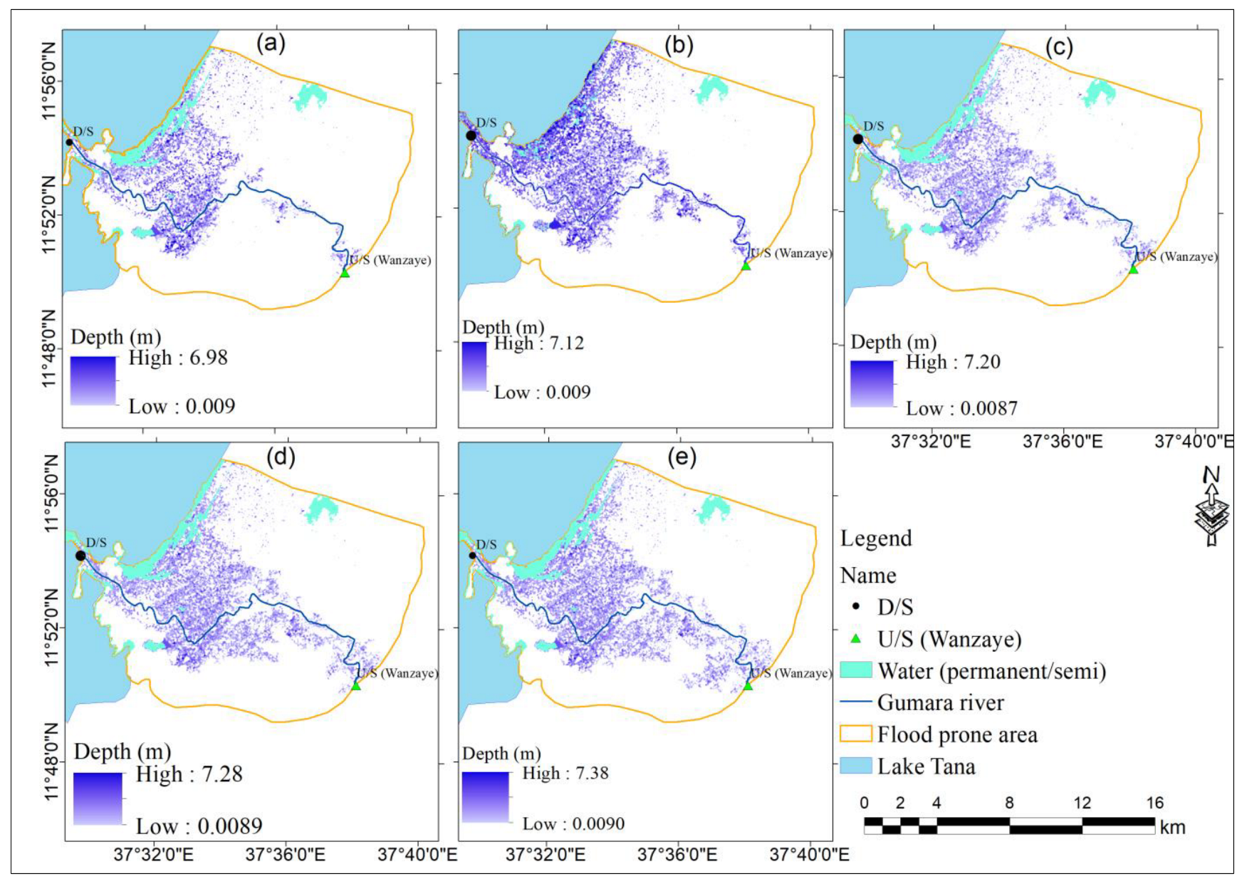
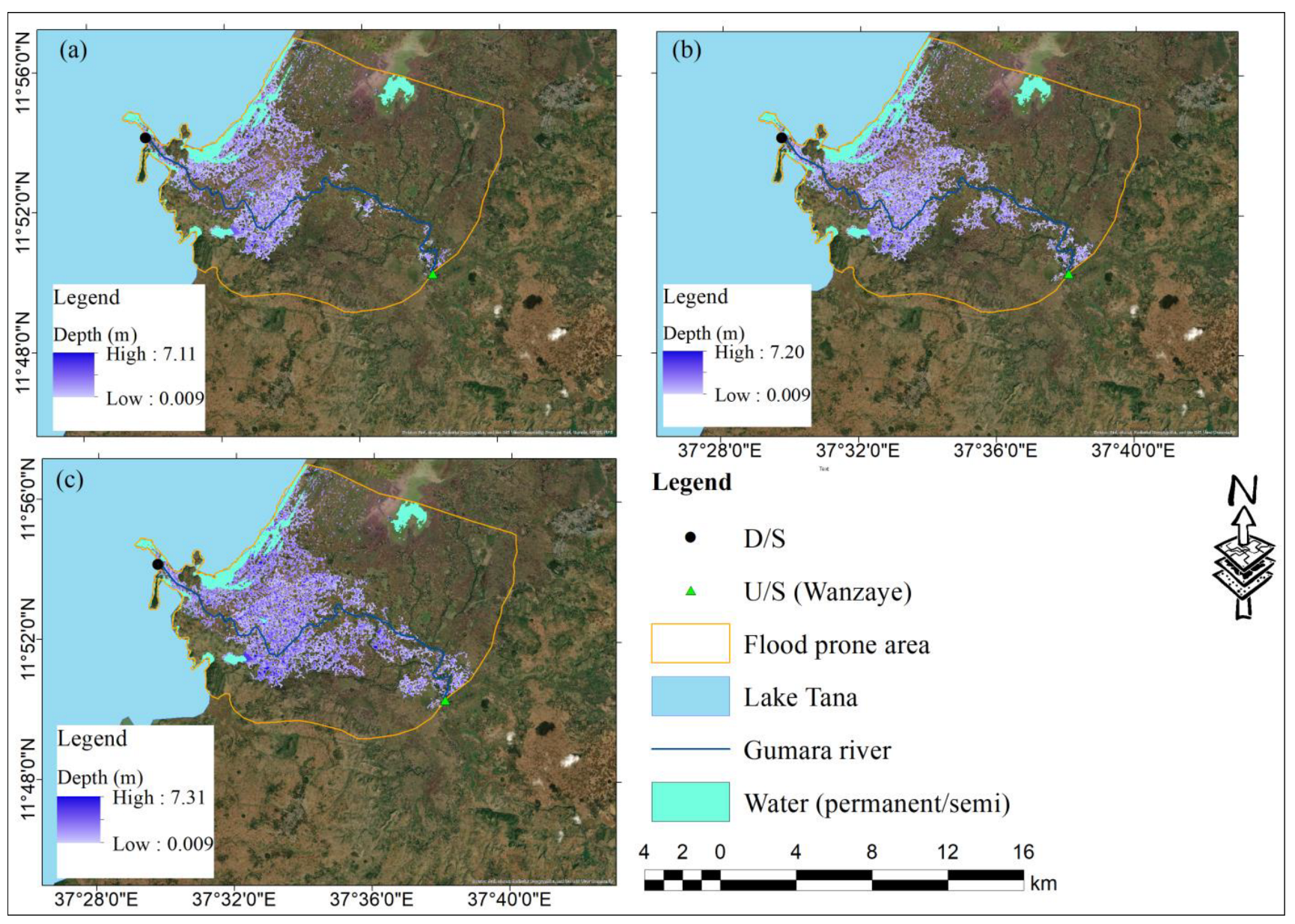
3.2.4. HEC-RAS Model-Simulated Flood Inundation Maps

Using the calibrated Manning’s n values summarized in Table 5, the HEC-RAS model was run for three flood events in 2019 (Figure 13). The resulting maps illustrate the spatial extent of flood inundation depth on each date, showing variations in flood extent due to differences in inflow conditions. According to the maps, the computed floods were primarily concentrated along the banks of the main river and near the shores of Lake Tana.

The simulation results revealed that the maximum flood depths on 22 July, 3 August, and 27 August 2019 were 7.20 m, 7.32 m, and 7.26 m, respectively (Figure 13a–c). The corresponding average flood depths were 0.89 m, 0.96 m, and 0.86 m. The flood inundation areas for these three events were estimated to be 29.46 km², 33.28 km², and 31.48 km², respectively. These findings highlight the consistency of the maximum flood depth, average flood depth, and inundation area, with the highest values occurring on 3 August, which coincided with the peak observed inflow. Additionally, the results align well with those of the SAR-based flood extent analysis, confirming that the maximum flood extent occurred on 3 August. Overall, these findings demonstrate the suitability of the HEC-RAS model for simulating flood inundation in the study region. Figure S5 in the Supplementary Materials further illustrates the variation in flood velocity over the floodplain area.

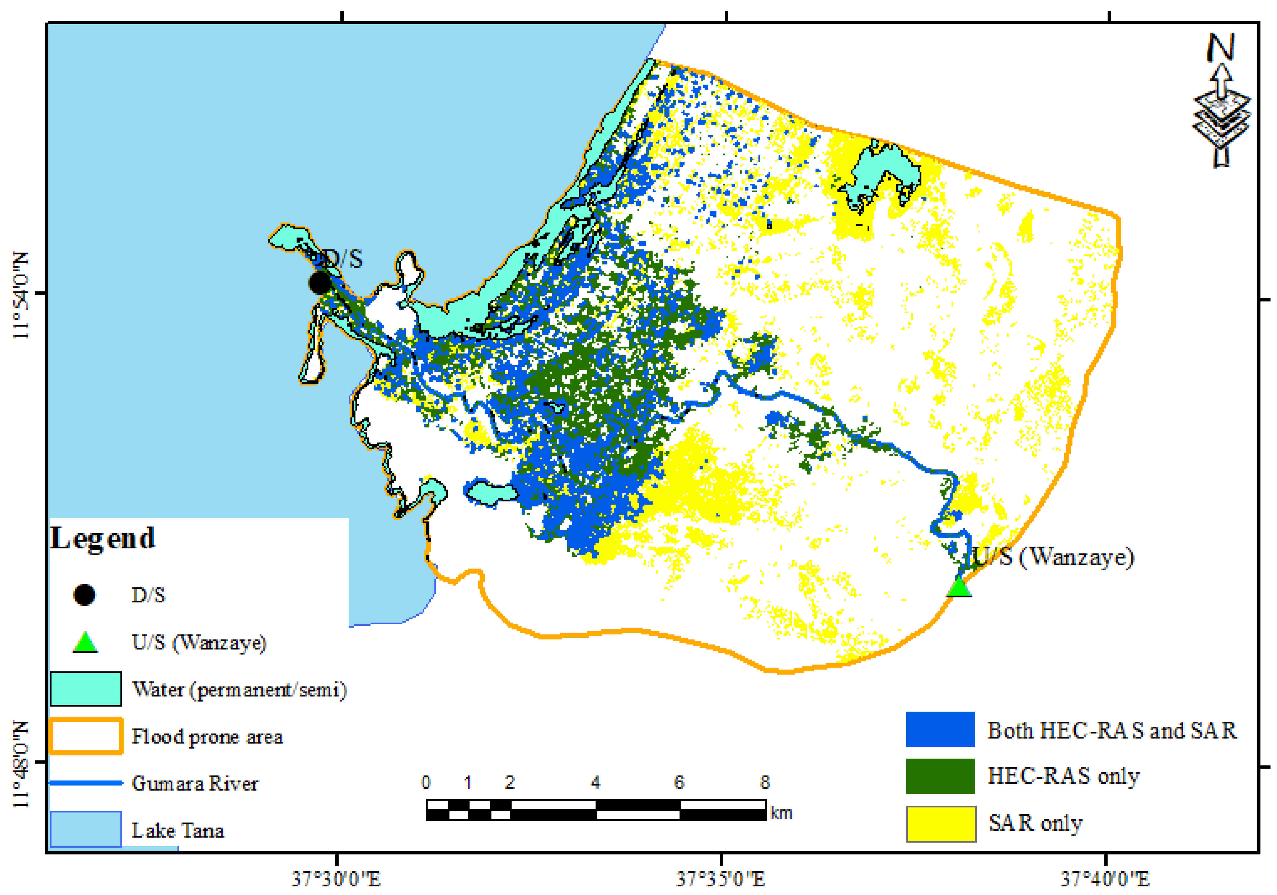
3.2.5. Model Validation

The HEC-RAS model flood inundation map was further validated via 300 ground control points (GCPs), comprising 150 points in flooded areas and 150 points in nonflooded areas. These GCPs were identified on the basis of Sentinel-2 imagery from 30 August 2019 and field investigations of frequently flood-affected areas, as described in the methods section. Figure 14a,b illustrate the HEC-RAS-derived flood inundation map and the spatial distributions of these GCPs used for model validation, respectively.

The confusion matrix (

Table 6. Confusion matrix for the validation of the HEC-RAS flood inundation map using ground control points (GCPs), and the corresponding accuracy assessment results.

HEC-RAS	Ground Control Points (Reference)
	Flooded	Nonflooded	∑	User’s Accuracy (%)	Commission Error (%)
Flooded	148	18	166	89.16	10.84
Nonflooded	23	111	134	82.84	17.16
∑	171	129	300
Producer’s accuracy (%)	86.55	86.05
Omission error (%)	13.45	13.95
Overall accuracy (%) Kappa coefficient	86.33 0.72

) summarizes the model’s accuracy compared with that of the GCPs. The $UA$ for flooded pixels was 89.16%, indicating that 89.16% of the pixels classified as flooded were correctly identified, whereas 10.84% were misclassified (commission error). Similarly, the $UA$ for nonflooded pixels was 82.84%, meaning that 17.16% of nonflooded pixels were misclassified. The $PA$ for the flooded pixels was 86.55%, indicating that 86.05% of the actual flooded pixels were correctly classified, whereas 13.45% were omitted (omission error). Similarly, the $PA$ for nonflooded pixels was 86.06%. Overall, the flood inundation maps generated via the HEC-RAS model demonstrated an $OA$ of 86.33% and a $K$ of 0.72, which can be considered substantial agreement according to Landis and Koch [75].

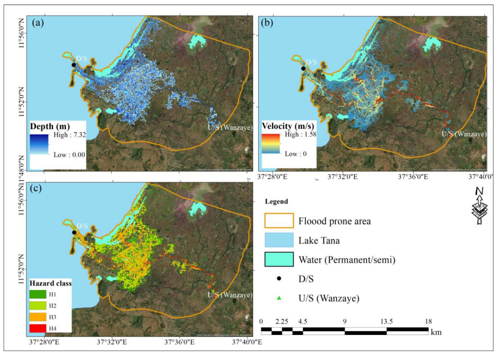
3.2.6. Flood Hazard Mapping

Flood hazard mapping is crucial for developing effective flood protection strategies and warning systems based on hazard levels. Depth and velocity are the most critical parameters in flood hazard mapping, as highlighted in several guidelines [72,76]. According to Brunner [56], these two factors are influenced primarily by elevation, surface roughness, and other floodplain characteristics.

In this study, the product of the computed depth (Figure 15a) and velocity (Figure 15b), termed the depth–velocity product (DVP), was used to classify flood hazard levels (H1 to H4) following the DEFRA [72] guidelines. The flood event on August 3, 2019 was selected for hazard classification as it represented the most extreme condition among the three flood events analyzed. The resulting flood hazard map (Figure 15c) indicates an extreme hazard level (H4) along and near the Gumara River channel, characterized by higher DVP values (DVP ≥ 2.5). In this area, the flood depth reached 7.32 m, and the flood velocity reached 1.58 m/s, leading to a relatively high DVP value. This extreme hazard level suggests severe flood damage in these areas. In contrast, the flatter parts of the floodplain presented varying hazard levels: low (H1), moderate (H2), and significant (H3). These findings align with those of previous studies by Anuthaman et al. [32] and Costabile et al. [39], who consistently reported extreme flood hazard levels along river channels and lower hazard levels in flatter floodplain regions. This pattern occurs because, during most flood events, water tends to accumulate in narrow river channels, leading to higher velocities due to the increased gravitational driving force [56]. Conversely, in flatter floodplain areas with relatively uniform elevations, both depth and velocity decrease as the gravitational force decreases [56]. Overall, the largest portion of the inundated area (approximately 45%) was categorized under the moderate hazard category (H2), whereas the smallest portion (approximately 8%) fell under the extreme hazard category (H4).

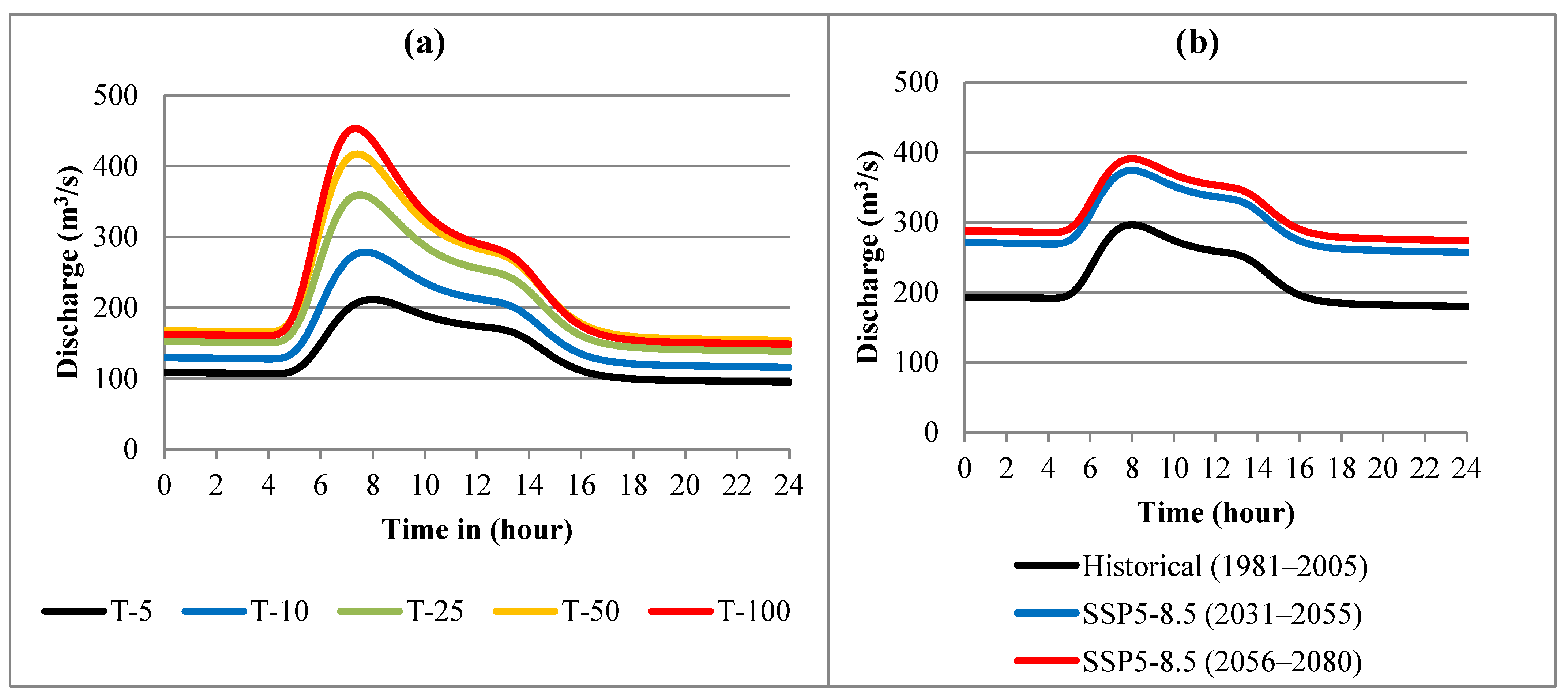
3.2.7. Flood Inundation Maps Under LULC and Climate Changes

Using the calibrated HEC-RAS model, flood simulations were conducted for different return periods (5, 10, 25, 50, and 100 years) via the inflow hydrographs presented in Figure 6a as the upstream boundary conditions. The resulting flood depth maps (Figure 16) revealed that areas near the Gumara River and along the shores of Lake Tana are particularly prone to flooding, with greater flood depths concentrated in these regions. In the computed maps, darker shades of blue indicate greater flood depths, whereas lighter shades of blue represent shallower flood depths. Overall, the simulations revealed average flood depths of 0.90, 0.92, 0.94, 0.97, and 1.02 m for the 5-, 10-, 25-, 50-, and 100-year return periods, respectively (

Table 7. Flood inundation extent and depth for different return periods.

Return Period (T)	Flooded Area (km2)	Flood Depth (m)
		Min	Max	Average
T-5	21.74	0.009	6.980	0.910
T-10	28.08	0.009	7.120	0.920
T-25	34.37	0.008	7.200	0.940
T-50	39.64	0.008	7.280	0.970
T-100	43.32	0.009	7.380	1.020

).

Similarly, via the calibrated HEC-RAS model, flood simulations were performed, with the inflow hydrographs presented in Figure 6b as the upstream boundary conditions for the historical and two future periods. Figure 17 shows the flood inundation maps generated for the historical (1981–2005), near-future (2031–2055), and far-future (2031–2055) periods under the SSP-8.5 climate scenario. The results revealed a consistent positive change (increase) in both the flood extent and average flood depth in the two future periods (

Table 8. Flood inundation extent and average flood depth and change analysis results between the historical and future periods.

Study Period	Flood Inundation Area (km2)	Change (%)	Average Flood Depth (m)	Change (%)
Historical (1981–2005)	28.09	–	0.92	–
SSP5-8.5 (2031–2055)	32.72	16.48	0.95	3.26
SSP5-8.5 (2056–2080)	35.74	27.23	0.98	6.52

). According to the results, the flood inundation extent is expected to increase by 16.48% and 27.23% in the near-future and far-future periods, respectively, relative to the historical period. Similarly, increases in the average flood depth of 3.26% and 6.52% are expected in the near-future and far-future periods, respectively. This increase in flood inundation area and depth is largely attributed to the greater magnitude of inflows expected in the future due to changes in LULC and climate conditions in the upstream watershed, as examined in our previous work [48]. Consistent with these findings, a study by [32,77,78] revealed an increase in flood occurrence under the combined effects of LULC and climate change.

3.2.8. Comparison of Flood Frequency Maps

To compare the flood inundation maps derived from SAR data and the HEC-RAS model, an overlay analysis was performed in ArcGIS for the 5-year return period. Figure 18 illustrates the flood extent captured exclusively by SAR data, exclusively by the HEC-RAS model, and their intersection. The results indicate that the overlapping area between both methods is larger than the flood extent captured by either method individually. The inundation analysis revealed that the average flood extent was 11.05 km² for SAR-derived data only, 5.24 km² for HEC-RAS model-derived data only, and approximately 16.60 km² for the intersection of both methods. As shown in Figure 18, the HEC-RAS model effectively captures flood inundation near the river and along the shores of Lake Tana. However, some flooded areas farther from the river were not captured by the HEC-RAS model. This discrepancy may be due to temporary water storage in depressions caused by excess rainfall rather than direct river overflow.

4. Discussion

4.1. SAR-Derived Flood Inundation Mapping

Near-real-time SAR-based flood inundation maps were generated via a change detection approach on the GEE cloud-based platform for specific flood events in 2019, as were time series of inundation data from 2017–2021. Change detection is the most commonly used and recommended approach for SAR-based flood mapping [10,79,80,81]. This method is flexible and can be implemented on the GEE platform by setting a threshold value for the difference image, which distinguishes flooded areas from nonflooded areas. Since inundation mapping via change detection is sensitive to the threshold due to variations in image reflectance, different threshold values were determined for the time-series flood inundation maps. In this study, optimal threshold values ranging from 1.25 to 1.40 were identified, which closely aligns with previous studies [9,21].

The SAR-derived flood inundation maps in this study adequately delineated frequently affected areas, which is consistent with the findings of a previous study conducted by Melkamu et al. [40]. However, a slight difference in the magnitude of the overall extent of the flood was observed. This can be attributed to differences in the timing of SAR image acquisition, the floodplain area considered, and the flood detection algorithm used. Specifically, Melkamu et al. [40] used SAR images acquired in July and August 2020, whereas this study utilized images from July and August 2019, along with composites from July to August, for time series inundation mapping. Additionally, Melkamu et al. [40] considered floodplain areas frequently affected by both the Gumara and Rib Rivers, whereas this study focused only on areas affected by the overflow of the Gumara River. Furthermore, Melkamu et al. [40] employed the Otsu thresholding algorithm [31], whereas this study used a change detection approach. The Otsu thresholding method [31] is mostly applied to classify single SAR images into flooded and nonflooded areas on the basis of backscatter intensity values. In contrast, the change detection approach compares preflood and postflood SAR images to identify areas where significant changes in backscatter intensity have occurred [28]. Therefore, change detection is often considered more flexible and robust, as it can track temporal changes rather than relying on intensity values from a single image [15,29,53].

Despite the importance of Sentinel-1 SAR-derived flood inundation maps for near-real-time flood mapping in the absence of observed flood data, several limitations exist [25,29]. For example, the acquisition of SAR images depends on satellite overpasses over specific areas, meaning that SAR sensors may miss fast or flash flood events due to their revisit times, which range from 6–12 days depending on the location. This limitation did not hinder this study, as the flood type in the Gumara watershed is characterized by riverine flooding, which typically has a longer progression and expansion time.

SAR sensors do not adequately capture floods under dense vegetation cover or in urban areas with structures [18,82]. In the Gumara watershed, more than 97% of the area is covered with cultivated land. Because of this, flood mapping was not hindered by this limitation of the SAR sensor. SAR images mostly suffer from speckle noise, which can affect the accuracy of flood mapping. In this study, this issue was addressed by applying the Lee speckle filter [49]. Furthermore, while SAR-derived flood maps provide valuable information about flood extent, they do not directly provide information on flood depth or velocity. These parameters are important for detailed flood hazard mapping. To address the limitations of SAR-based flood inundation mapping, this study employed the HEC-RAS 2D model, which allows for a more comprehensive flood analysis by simulating not only the extent but also the depth and velocity of floodwaters. This combination of SAR images and hydraulic modeling could improve the accuracy of flood risk mapping [10,37].

4.2. HEC-RAS 2D Flood Modeling

In the HEC-RAS 2D model, the DW equations were chosen to compute flood depth and velocity over the 2D flow area. This method was selected because it does not demand high computational resources and has a shorter run time than the full SW equations [39,56]. Additionally, the DW approach provides high numerical stability and is well-suited for simulating floods in relatively flat floodplain areas, such as the study area considered in this research [64,83].

The computed flood maps in HEC-RAS effectively delineated frequently affected areas, which is consistent with studies conducted by Melkamu et al. [40] and Nigusie et al. [43]. However, slight differences were observed in the magnitude of flood depth and velocity. These variations could be attributed to differences in the flood-prone area considered, the terrain model resolution, the 2D computational mesh spacing, Manning’s roughness n value, and other related parameters.

Unlike previous studies conducted in the area, this study incorporated a modified terrain model to account for flood propagation through the river channel and calibrated Manning’s roughness n values to increase the accuracy of flood depth and velocity estimates. Additionally, the impacts of LULC and climate changes in the upland watershed were considered, and their influences on flood depth and flood extent in the floodplain for various return periods were examined. This was achieved using inflow hydrographs computed under different LULC and climate conditions as upstream boundary conditions [48]. The results revealed an increase in flood depth and extent in future periods, potentially intensifying the flood risk in the area. Similar studies have reported increases in flood depth and extent due to land use changes, such as deforestation, agricultural expansion, and urbanization, as well as extreme rainfall events [66,84,85,86].

The HEC-RAS 2D model provides detailed information on flood dynamics but has several limitations. For example, the simulation time may be longer than that of SAR-derived flood inundation mapping because detailed topographic and hydraulic input data are needed [36,38]. To address this limitation, this study utilized a modified terrain model. Furthermore, while HEC-RAS 2D simulation is primarily appropriate for smaller basins or watersheds, it may not be recommended for large-scale flood mapping.

In summary, despite their limitations, both the SAR-derived and HEC-RAS-computed flood inundation maps for the study area provide valuable information on the spatial and temporal distributions, extent, and progression of the flood. These maps can assist watershed managers, policymakers, environmentalists, and other stakeholders in developing early warning systems, designing sustainable flood protection and management strategies, and mitigating the impacts of flooding. Overall, to mitigate future flood risks in downstream areas, implementing sustainable land use practices, including reforestation and controlled agricultural cultivation, along with improved water management strategies to reduce the impact of extreme rainfall events on flooding, is recommended.

4.3. Future Research Directions

This study used Sentinel-1 SAR data for flood inundation mapping in the region. Future research could enhance flood mapping accuracy by incorporating multisource satellite imagery, such as Sentinel-2 and Landsat imagery, through a multisource data fusion approach.

The 2D hydrodynamic flood modeling in HEC-RAS in this study was performed via the DW equation, an approximation of the SW equation, owing to computational resource and data availability constraints. Future studies could explore the application of the full SW equation, utilize high-performance computing resources to account for acceleration in addition to primary governing forces (gravitational and friction forces), and compare the results with those obtained via the DW equation.

High-resolution elevation data are crucial for accurately estimating flood depths and velocities in flood modeling. In this study, a modified terrain DEM with a 12.5 m resolution was used, as higher-resolution data for the area were not available. Future studies could benefit from incorporating high-resolution light detection and ranging (LiDAR) data to improve flood mapping in the region.

Additionally, further research on the socioeconomic impacts of flooding, along with the development and assessment of adaptive flood protection measures, is essential for enhancing resilience in flood-prone areas.

5. Conclusions

This study focused on generating near-real-time flood maps, flood inundation maps for different return periods, and future flood inundation scenarios for the downstream part of the Gumara watershed. Near-real-time flood inundation mapping was conducted via Sentinel-1 SAR images on the GEE cloud-based platform for flood events that occurred from 2017–2021. Among these, flood events on 22 July, 3 August, and 27 August 2019 were used to calibrate the HEC-RAS 2D model. SAR-based flood mapping was performed via a change detection approach followed by histogram thresholding of the difference image. The analysis revealed that the optimal threshold value for distinguishing flooded pixels ranged from 1.25–1.4.

A 2D hydraulic flood model was developed via HEC-RAS. Model sensitivity analysis was conducted by varying Manning’s roughness coefficient (n), the primary parameter influencing 2D flood modeling. Model calibration was performed by comparing simulated flood maps with SAR-derived flood maps. Overall, considering the three calibration events, the model performance improved in terms of the F-score (from 0.54 to 0.57), OA (from 85.66% to 86.92%), and K (from 0.59 to 0.62). Further validation using ground control points (GCPs) resulted in an OA of 89.16% and a K of 0.72, indicating the model’s effectiveness in simulating floods in the study region.

Using the calibrated model, flood inundation maps were generated for different return periods (5, 10, 25, 50, and 100 years). Additionally, future flood inundation scenarios were developed for the near-future and far-future periods. The results indicated a projected increase in the flood inundation area of 16.48% in the near future and 27.23% in the far future compared with the historical period. This increase is attributed to the combined effects of LULC changes and the intensification of extreme rainfall events due to climate change in the upstream watershed.

The flood inundation maps derived from SAR imagery and HEC-RAS modeling provide valuable information for watershed managers and decision-makers in designing effective flood risk mitigation structures. Future research could enhance flood mapping accuracy by integrating multisource satellite imagery, such as Sentinel-2 and Landsat imagery, through a data fusion approach. Additionally, applying the full SW equation in 2D hydrodynamic modeling, coupled with high-performance computing, could yield more detailed results than the DW approximation. The incorporation of high-resolution LiDAR data would improve flood depth and velocity estimates. Further studies should also focus on assessing the socioeconomic impacts of flooding and developing adaptive flood protection measures to increase resilience in flood-prone areas.

References

1. Kundzewicz, Z.W.; Kanae, S.; Seneviratne, S.I.; Handmer, J.; Nicholls, N.; Peduzzi, P.; Mechler, R.; Bouwer, L.M.; Arnell, N.; Mach, K. Flood Risk and Climate Change: Global and Regional Perspectives. Hydrol. Sci. J. 2014, 59, 1–28. [Google Scholar]
2. Taye, M.T.; Dyer, E. Hydrologic Extremes in a Changing Climate: A Review of Extremes in East Africa. Curr. Clim. Change Rep. 2024, 10, 1–11. [Google Scholar] [CrossRef]
3. Kwakye, S.O.; Bárdossy, A. Quantification of the Hydrological Consequences of Climate Change in a Typical West African Catchment Using Flow Duration Curves. J. Water Clim. Change 2022, 13, 26–42. [Google Scholar] [CrossRef]
4. Getahun, Y.S.; Gebre, S.L. Flood Hazard Assessment and Mapping of Flood Inundation Area of the Awash River Basin in Ethiopia Using GIS and HEC-GeoRAS/HEC-RAS Model. J. Civ. Environ. Eng. 2015, 5, 1. [Google Scholar]
5. Fekadu, A. Detecting Flash Flood Hazard Areas Using Geo-Spatial–Based Analytic Hierarchy Process in Weidie Watershed South Western Ethiopia. J. Remote Sens. GIS 2018, 7, 1–5. [Google Scholar] [CrossRef]
6. Adane, G.B.; Kassa, A.K.; Toni, A.T.; Tekle, S.L. Spatial Runoff Estimation under Different Land Uses and Rainfall Frequencies: Case of Flood-Prone Dechatu River Catchment, Dire Dawa, Ethiopia. Arab. J. Geosci. 2022, 15, 1092. [Google Scholar]
7. Belay, H.; Melesse, A.M.; Tegegne, G. Evaluation and Comparison of the Performances of the CMIP5 and CMIP6 Models in Reproducing Extreme Rainfall in the Upper Blue Nile Basin of Ethiopia. Theor. Appl. Climatol. 2024, 155, 9471–9496. [Google Scholar] [CrossRef]
8. United Nations Office for the Coordination of Humanitarian Affairs (OCHA). Eastern Africa Region: Regional Floods Snapshot. 2019. Available online: https://reliefweb.int/report/south-sudan/eastern-africa-region-regional-flood-snapshot-november-2019 (accessed on 20 March 2024).
9. Pandey, A.C.; Kaushik, K.; Parida, B.R. Google Earth Engine for Large-Scale Flood Mapping Using SAR Data and Impact Assessment on Agriculture and Population of Ganga-Brahmaputra Basin. Sustainability 2022, 14, 4210. [Google Scholar] [CrossRef]
10. Psomiadis, E.; Diakakis, M.; Soulis, K.X. Combining SAR and Optical Earth Observation with Hydraulic Simulation for Flood Mapping and Impact Assessment. Remote Sens. 2020, 12, 3980. [Google Scholar] [CrossRef]
11. Elkhrachy, I.; Pham, Q.B.; Costache, R.; Mohajane, M.; Rahman, K.U.; Shahabi, H.; Linh, N.T.T.; Anh, D.T. Sentinel-1 Remote Sensing Data and Hydrologic Engineering Centres River Analysis System Two-Dimensional Integration for Flash Flood Detection and Modelling in New Cairo City, Egypt. J. Flood Risk Manag. 2021, 14, e12692. [Google Scholar] [CrossRef]
12. Ouled Sghaier, M.; Hammami, I.; Foucher, S.; Lepage, R. Flood Extent Mapping from Time-Series SAR Images Based on Texture Analysis and Data Fusion. Remote Sens. 2018, 10, 237. [Google Scholar] [CrossRef]
13. Tiwari, V.; Kumar, V.; Matin, M.A.; Thapa, A.; Ellenburg, W.L.; Gupta, N.; Thapa, S. Flood Inundation Mapping-Kerala 2018; Harnessing the Power of SAR, Automatic Threshold Detection Method and Google Earth Engine. PLoS ONE 2020, 15, e0237324. [Google Scholar] [CrossRef]
14. Kumar, H.; Karwariya, S.K.; Kumar, R. Google Earth Engine-Based Identification of Flood Extent and Flood-Affected Paddy Rice Fields Using Sentinel-2 MSI and Sentinel-1 SAR Data in Bihar State, India. J. Indian Soc. Remote Sens. 2022, 50, 791–803. [Google Scholar] [CrossRef]
15. Tay, C.W.J.; Yun, S.H.; Chin, S.T.; Bhardwaj, A.; Jung, J.; Hill, E.M. Rapid Flood and Damage Mapping Using Synthetic Aperture Radar in Response to Typhoon Hagibis, Japan. Sci. Data 2020, 7, 100. [Google Scholar] [CrossRef]
16. Anusha, N.; Bharathi, B. Flood Detection and Flood Mapping Using Multi-Temporal Synthetic Aperture Radar and Optical Data. Egypt. J. Remote Sens. Sp. Sci. 2020, 23, 207–219. [Google Scholar]
17. Pulvirenti, L.; Chini, M.; Pierdicca, N.; Guerriero, L.; Ferrazzoli, P. Flood Monitoring Using Multi-Temporal COSMO-SkyMed Data: Image Segmentation and Signature Interpretation. Remote Sens. Environ. 2011, 115, 990–1002. [Google Scholar]
18. Grimaldi, S.; Xu, J.; Li, Y.; Pauwels, V.R.N.; Walker, J.P. Flood Mapping under Vegetation Using Single SAR Acquisitions. Remote Sens. Environ. 2020, 237, 111582. [Google Scholar] [CrossRef]
19. Twele, A.; Cao, W.; Plank, S.; Martinis, S. Sentinel-1-Based Flood Mapping: A Fully Automated Processing Chain. Int. J. Remote Sens. 2016, 37, 2990–3004. [Google Scholar]
20. Aldiansyah, S.; Saputra, R.A.; Wahid, K.A.; Madani, I.; Setiyo, D. Rapid Flood Inundation Mapping Using Multi-Temporal Sentinel-1 SAR: An Example from Kendari City. J. Geosains Dan Remote Sens. 2024, 5, 15–26. [Google Scholar] [CrossRef]
21. Singh, G.; Rawat, K.S. Mapping Flooded Areas Utilizing Google Earth Engine and Open SAR Data: A Comprehensive Approach for Disaster Response. Discov. Geosci. 2024, 2, 5. [Google Scholar] [CrossRef]
22. Nghia, B.P.Q.; Pal, I.; Chollacoop, N.; Mukhopadhyay, A. Applying Google Earth Engine for Flood Mapping and Monitoring in the Downstream Provinces of Mekong River. Prog. Disaster Sci. 2022, 14, 100235. [Google Scholar] [CrossRef]
23. Passah, A.; Sur, S.N.; Abraham, A.; Kandar, D. Synthetic Aperture Radar Image Analysis Based on Deep Learning: A Review of a Decade of Research. Eng. Appl. Artif. Intell. 2023, 123, 106305. [Google Scholar]
24. Gorelick, N.; Hancher, M.; Dixon, M.; Ilyushchenko, S.; Thau, D.; Moore, R. Google Earth Engine: Planetary-Scale Geospatial Analysis for Everyone. Remote Sens. Environ. 2017, 202, 18–27. [Google Scholar]
25. Amitrano, D.; Di Martino, G.; Di Simone, A.; Imperatore, P. Flood Detection with SAR: A Review of Techniques and Datasets. Remote Sens. 2024, 16, 656. [Google Scholar] [CrossRef]
26. Perera, E.D.P.; Lahat, L. Fuzzy Logic Based Flood Forecasting Model for the Kelantan River Basin, Malaysia. J. Hydro-Environ. Res. 2015, 9, 542–553. [Google Scholar]
27. Nobre, A.D.; Cuartas, L.A.; Momo, M.R.; Severo, D.L.; Pinheiro, A.; Nobre, C.A. HAND Contour: A New Proxy Predictor of Inundation Extent. Hydrol. Process. 2016, 30, 320–333. [Google Scholar]
28. Clement, M.A.; Kilsby, C.G.; Moore, P. Multi-Temporal Synthetic Aperture Radar Flood Mapping Using Change Detection. J. Flood Risk Manag. 2018, 11, 152–168. [Google Scholar] [CrossRef]
29. Giustarini, L.; Hostache, R.; Matgen, P.; Schumann, G.J.-P.; Bates, P.D.; Mason, D.C. A Change Detection Approach to Flood Mapping in Urban Areas Using TerraSAR-X. IEEE Trans. Geosci. Remote Sens. 2012, 51, 2417–2430. [Google Scholar]
30. Long, S.; Fatoyinbo, T.E.; Policelli, F. Flood Extent Mapping for Namibia Using Change Detection and Thresholding with SAR. Environ. Res. Lett. 2014, 9, 035002. [Google Scholar] [CrossRef]
31. Otsu, N. A Threshold Selection Method from Gray-Level Histograms. Automatica 1975, 11, 23–27. [Google Scholar]
32. Anuthaman, S.N.; Ramasamy, S.; Lakshminarayanan, B.; Ramasubbu, B. Modelling and Forecasting of Urban Flood under Changing Climate and Land Use Land Cover. J. Water Clim. Change 2023, 14, 4314–4335. [Google Scholar] [CrossRef]
33. Mzava, P.; Valimba, P.; Nobert, J. Quantitative Analysis of the Impacts of Climate and Land-Cover Changes on Urban Flood Runoffs: A Case of Dar Es Salaam, Tanzania. J. Water Clim. Change 2021, 12, 2835–2853. [Google Scholar] [CrossRef]
34. Brunner, G.W. HEC-RAS HEC-RAS 2D User ’ s Manual. U.S. Army Corps Eng. 2024, 6.5, 1–272. [Google Scholar]
35. Rangari, V.A.; Umamahesh, N.V.; Bhatt, C.M. Assessment of Inundation Risk in Urban Floods Using HEC RAS 2D. Model. Earth Syst. Environ. 2019, 5, 1839–1851. [Google Scholar] [CrossRef]
36. Quirogaa, V.M.; Kurea, S.; Udoa, K.; Manoa, A. Application of 2D Numerical Simulation for the Analysis of the February 2014 Bolivian Amazonia Flood: Application of the New HEC-RAS Version 5. Ribagua 2016, 3, 25–33. [Google Scholar] [CrossRef]
37. Ezzine, A.; Saidi, S.; Hermassi, T.; Kammessi, I.; Darragi, F.; Rajhi, H. Flood Mapping Using Hydraulic Modeling and Sentinel-1 Image: Case Study of Medjerda Basin, Northern Tunisia. Egypt. J. Remote Sens. Sp. Sci. 2020, 23, 303–310. [Google Scholar] [CrossRef]
38. Ongdas, N.; Akiyanova, F.; Karakulov, Y.; Muratbayeva, A.; Zinabdin, N. Application of Hec-Ras (2d) for Flood Hazard Maps Generation for Yesil (Ishim) River in Kazakhstan. Water 2020, 12, 2672. [Google Scholar] [CrossRef]
39. Costabile, P.; Costanzo, C.; Ferraro, D.; Macchione, F.; Petaccia, G. Performances of the New HEC-RAS Version 5 for 2-D Hydrodynamic-Based Rainfall-Runoff Simulations at Basin Scale: Comparison with a State-of-the Art Model. Water 2020, 12, 2326. [Google Scholar] [CrossRef]
40. Melkamu, T.; Bagyaraj, M.; Adimaw, M.; Ngusie, A. Detecting and Mapping Flood Inundation Areas in Fogera-Dera Floodplain, Ethiopia during an Extreme Wet Season Using Sentinel-1 Data. Phys. Chem. Earth Parts a/b/c 2022, 127, 103189. [Google Scholar] [CrossRef]
41. Alemu, D.; Assaye, A. Devastating Effect of Floods on Rice Production and Commercialization in the Fogera Plain; Future Agricultures Consortium Secretariat: Brighton, UK, 2020. [Google Scholar]
42. Gashaw, W.; Legesse, D. Flood Hazard and Risk Assessment Using GIS and Remote Sensing in Fogera Woreda, Northwest Ethiopia. Nile River Basin 2011, 6, 179–206. [Google Scholar] [CrossRef]
43. Nigusie, A.A.; Shiferaw, K.M.; Ebrahim, S.E. Flood Inundation Modeling Using HEC-RAS: The Case of Downstream Gumara River, Lake Tana Sub Basin, Ethiopia. Geocarto Int. 2021, 37, 9625–9643. [Google Scholar] [CrossRef]
44. Belay, H.; Melesse, A.M.; Tegegne, G. Scenario-Based Land Use and Land Cover Change Detection and Prediction Using the Cellular Automata–Markov Model in the Gumara Watershed, Upper Blue Nile Basin, Ethiopia. Land 2024, 13, 396. [Google Scholar] [CrossRef]
45. Chakilu, G.G.; Moges, M.A. Assessing the Land Use/Cover Dynamics and Its Impact on the Low Flow of Gumara Watershed, Upper Blue Nile Basin, Ethiopia. Hydrol. Curr. Res. 2017, 8, 268. [Google Scholar] [CrossRef]
46. Dawit, M.; Halefom, A.; Teshome, A.; Sisay, E.; Shewayirga, B.; Dananto, M. Changes and Variability of Precipitation and Temperature in the Guna Tana Watershed, Upper Blue Nile Basin, Ethiopia. Model. Earth Syst. Environ. 2019, 5, 1395–1404. [Google Scholar] [CrossRef]
47. Pekel, J.-F.; Cottam, A.; Gorelick, N.; Belward, A.S. High-Resolution Mapping of Global Surface Water and Its Long-Term Changes. Nature 2016, 540, 418–422. [Google Scholar] [CrossRef]
48. Belay, H.; Melesse, A.M.; Tegegne, G.; Tamiru, H. Identifying Flood Source Areas and Analyzing High-Flow Extremes Under Changing Land Use, Land Cover, and Climate in the Gumara Watershed, Upper Blue Nile Basin, Ethiopia. Climate 2025, 13, 7. [Google Scholar] [CrossRef]
49. Lee, J.-S.; Jurkevich, L.; Dewaele, P.; Wambacq, P.; Oosterlinck, A. Speckle Filtering of Synthetic Aperture Radar Images: A Review. Remote Sens. Rev. 1994, 8, 313–340. [Google Scholar]
50. Filipponi, F. Sentinel-1 GRD Preprocessing Workflow. In Proceedings of the Proceedings; MDPI: Basel, Switzerland, 2019; Volume 18, p. 11. [Google Scholar]
51. United Nations Platform for Space-based Information for Disaster Management and Emergency Response (UN-SPIDER). Step by Step: Recommended Practice Flood Mapping. Available online: https://www.un-spider.org/advisory-support/recommended-practices/recommended-practice-flood-mapping/step-by-step (accessed on 1 March 2024).
52. Loukili, Y.; Lakhrissi, Y.; Ali, S.E. Ben Flood Mapping Methodologies in Google Earth Engine Using Optical and Radar Data: A Comparative Study. J. Environ. Earth Sci. 2025, 7, 363–380. [Google Scholar] [CrossRef]
53. Tupas, M.E.; Roth, F.; Bauer-Marschallinger, B.; Wagner, W. An Intercomparison of Sentinel-1 Based Change Detection Algorithms for Flood Mapping. Remote Sens. 2023, 15, 1200. [Google Scholar] [CrossRef]
54. Notti, D.; Giordan, D.; Caló, F.; Pepe, A.; Zucca, F.; Galve, J.P. Potential and Limitations of Open Satellite Data for Flood Mapping. Remote Sens. 2018, 10, 1673. [Google Scholar] [CrossRef]
55. Akiyanova, F.; Ongdas, N.; Zinabdin, N.; Karakulov, Y.; Nazhbiyev, A.; Mussagaliyeva, Z.; Atalikhova, A. Operation of Gate-Controlled Irrigation System Using HEC-RAS 2D for Spring Flood Hazard Reduction. Computation 2023, 11, 27. [Google Scholar] [CrossRef]
56. Brunner, G.W. HEC-RAS HEC-RAS Hydraulic Reference. U.S. Army Corps Eng. 2024, 6.5, 1–477. [Google Scholar]
57. Chaudhry, M.H. Open-Channel Flow; Springer: Berlin/Heidelberg, Germany, 2008; Volume 523. [Google Scholar]
58. Robinson, D.; Zundel, A.; Kramer, C.; Nelson, R.; deRosset, W.; Hunt, J.; Hogan, S.; Lai, Y.; Aquaveo, L.L.C. Two-Dimensional Hydraulic Modeling for Highways in the River Environment: Reference Document; Federal Highway Administration (US): Washington, DC, USA, 2019. [Google Scholar]
59. Mekuria, W.; Mekonnen, K.; Thorne, P.; Bezabih, M.; Tamene, L.; Abera, W. Competition for Land Resources: Driving Forces and Consequences in Crop-Livestock Production Systems of the Ethiopian Highlands. Ecol. Process. 2018, 7, 30. [Google Scholar] [CrossRef]
60. Casulli, V. A High-resolution Wetting and Drying Algorithm for Free-surface Hydrodynamics. Int. J. Numer. Methods Fluids 2009, 60, 391–408. [Google Scholar]
61. Chow, V.T. Open-Channel Hydraulics; McGraw-Hill: New York, NY, USA, 1959. [Google Scholar]
62. Hirsch, C. Computational methods for inviscid and viscous flows. In Numerical Computation of Internal and External Flows; Wiley: Hoboken, NJ, USA, 1990; Volume 2. [Google Scholar]
63. Tsubaki, R.; Kawahara, Y. The Uncertainty of Local Flow Parameters during Inundation Flow over Complex Topographies with Elevation Errors. J. Hydrol. 2013, 486, 71–87. [Google Scholar] [CrossRef]
64. Ghimire, E.; Sharma, S.; Lamichhane, N. Evaluation of One-Dimensional and Two-Dimensional HEC-RAS Models to Predict Flood Travel Time and Inundation Area for Flood Warning System ABSTRACT. ISH J. Hydraul. Eng. 2020, 28, 110–126. [Google Scholar] [CrossRef]
65. Farooq, M.; Shafique, M.; Shahzad, M. Flood Hazard Assessment and Mapping of River Swat Using HEC—RAS 2D Model and High-Resolution 12-m TanDEM-X DEM. Nat. Hazards 2019, 97, 477–492. [Google Scholar] [CrossRef]
66. Madhuri, R.; Raja, Y.S.L.S.; Raju, K.S.; Punith, B.S.; Manoj, K. Urban Flood Risk Analysis of Buildings Using HEC-RAS 2D in Climate Change Framework. H2Open J. 2021, 4, 262–275. [Google Scholar]
67. Afzal, M.A.; Ali, S.; Nazeer, A.; Khan, M.I.; Waqas, M.M.; Aslam, R.A.; Cheema, M.J.M.; Nadeem, M.; Saddique, N.; Muzammil, M.; et al. Flood Inundation Modeling by Integrating HEC–RAS and Satellite Imagery: A Case Study of the Indus River Basin. Water 2022, 14, 2984. [Google Scholar] [CrossRef]
68. Minh, V.A.; Quang, D.N.; Tinh, N.X.; Ribbe, L. Spatio-Temporal Dynamics Monitoring of Surface Water Bodies in Nhat Le River Basin, Vietnam, by Google Earth Engine. J. Water Clim. Change 2024, 15, 1262–1281. [Google Scholar] [CrossRef]
69. Peng, X.; Chen, S.; Miao, Z.; Xu, Y.; Ye, M.; Lu, P. Automatic Flood Monitoring Method with SAR and Optical Data Using Google Earth Engine. Water 2025, 17, 177. [Google Scholar] [CrossRef]
70. Johary, R.; Révillion, C.; Catry, T.; Alexandre, C.; Mouquet, P.; Rakotoniaina, S.; Pennober, G.; Rakotondraompiana, S. Detection of Large-Scale Floods Using Google Earth Engine and Google Colab. Remote Sens. 2023, 15, 5368. [Google Scholar] [CrossRef]
71. Song, L.; Song, C.; Luo, S.; Chen, T.; Liu, K.; Li, Y.; Jing, H.; Xu, J. Refining and Densifying the Water Inundation Area and Storage Estimates of Poyang Lake by Integrating Sentinel-1/2 and Bathymetry Data. Int. J. Appl. Earth Obs. Geoinf. 2021, 105, 102601. [Google Scholar] [CrossRef]
72. United Kingdom Department for Environment, Food, and Rural Affairs (DEFRA). Flood Risk Assessment Guidance for New Development—Phase 2—Technical Report 1. 2005. Available online: http://sciencesearch.defra.gov.uk/Document.aspx?Document=FD2320_3363_TRP.pdf (accessed on 25 March 2024).
73. Mason, D.C.; Speck, R.; Devereux, B.; Schumann, G.J.-P.; Neal, J.C.; Bates, P.D. Flood Detection in Urban Areas Using TerraSAR-X. IEEE Trans. Geosci. Remote Sens. 2009, 48, 882–894. [Google Scholar]
74. Dimitriadis, P.; Tegos, A.; Oikonomou, A.; Pagana, V.; Koukouvinos, A.; Mamassis, N.; Koutsoyiannis, D.; Efstratiadis, A. Comparative Evaluation of 1D and Quasi-2D Hydraulic Models Based on Benchmark and Real-World Applications for Uncertainty Assessment in Flood Mapping. J. Hydrol. 2016, 534, 478–492. [Google Scholar] [CrossRef]
75. Landis, J.R.; Koch, G.G. The Measurement of Observer Agreement for Categorical Data. Biometrics 1977, 33, 159–174. [Google Scholar]
76. FEMA (Federal Emergency Management Agency). Map Modernization, Guidelines, and Specifications for Flood Hazard Mapping Partners. 2003. Available online: https://www.fema.gov/ (accessed on 15 March 2024).
77. Yang, S.; Yang, D.; Zhao, B.; Ma, T.; Lu, W.; Santisirisomboon, J. Future Changes in High and Low Flows under the Impacts of Climate and Land Use Changes in the Jiulong River Basin of Southeast China. Atmosphere 2022, 13, 150. [Google Scholar] [CrossRef]
78. Akter, T.; Quevauviller, P.; Eisenreich, S.J.; Vaes, G. Impacts of Climate and Land Use Changes on Flood Risk Management for the Schijn River, Belgium. Environ. Sci. Policy 2018, 89, 163–175. [Google Scholar] [CrossRef]
79. Huang, M.; Jin, S. Rapid Flood Mapping and Evaluation with a Supervised Classifier and Change Detection in Shouguang Using Sentinel-1 SAR and Sentinel-2 Optical Data. Remote Sens. 2020, 12, 2073. [Google Scholar] [CrossRef]
80. Li, Y.; Martinis, S.; Plank, S.; Ludwig, R. An Automatic Change Detection Approach for Rapid Flood Mapping in Sentinel-1 SAR Data. Int. J. Appl. earth Obs. Geoinf. 2018, 73, 123–135. [Google Scholar]
81. Zhao, M.; Ling, Q.; Li, F. An Iterative Feedback-Based Change Detection Algorithm for Flood Mapping in SAR Images. IEEE Geosci. Remote Sens. Lett. 2018, 16, 231–235. [Google Scholar]
82. Tanim, A.H.; McRae, C.B.; Tavakol-Davani, H.; Goharian, E. Flood Detection in Urban Areas Using Satellite Imagery and Machine Learning. Water 2022, 14, 1140. [Google Scholar] [CrossRef]
83. Nasiri, V.; Deljouei, A.; Moradi, F.; Sadeghi, S.M.M.; Borz, S.A. Land Use and Land Cover Mapping Using Sentinel-2, Landsat-8 Satellite Images, and Google Earth Engine: A Comparison of Two Composition Methods. Remote Sens. 2022, 14, 1977. [Google Scholar] [CrossRef]
84. Chen, Q.; Chen, H.; Zhang, J.; Hou, Y.; Shen, M.; Chen, J.; Xu, C. Impacts of Climate Change and LULC Change on Runoff in the Jinsha River Basin. J. Geogr. Sci. 2020, 30, 85–102. [Google Scholar] [CrossRef]
85. Saghafian, B.; Farazjoo, H.; Bozorgy, B.; Yazdandoost, F. Flood Intensification Due to Changes in Land Use. Water Resour. Manag. 2008, 22, 1051–1067. [Google Scholar] [CrossRef]
86. Lane, R.A.; Kay, A.L. Climate Change Impact on the Magnitude and Timing of Hydrological Extremes Across Great Britain. Front. Water 2021, 3, 684982. [Google Scholar] [CrossRef]
Figure 1. Location map of the study area. (a) The Upper Blue Nile (UBN) Basin and the Lake Tana sub-basin within the context of Ethiopia’s 12 river basins, (b) the Gumara watershed in the context of the Lake Tana sub-basin, and (c) detailed features of the study area, including the streamflow gauging station, flood-prone area, Gumara River (downstream section), and elevation map. The yellow box in subfigure (b) highlights the flood prone area.
Remotesensing 17 01283 g001
Figure 2. (a) Mean monthly rainfall of the Gumara watershed (1981–2019) and (b) mean monthly streamflow of the Gumara River at the Wanzaye gauging station (1981–2019).
Remotesensing 17 01283 g002
Figure 3. Overall methodological framework of this study.
Remotesensing 17 01283 g003
Figure 4. Terrain modification in triangular irregular (TIN) format. (a) Original terrain model, (b) modified terrain model, and (c) details of the modified terrain model showing the Gumara River (channel) and elevation variation in the floodplain area found at the left bank of the river. The red box shows a snapshot of the floodplain area detailed in (c).
Remotesensing 17 01283 g004
Figure 5. Boundary conditions and land use/land cover (LULC) map of the floodplain area for 2019. In the legend, the values indicated in brackets represent the ranges of Manning’s n values corresponding to different LULC classes, as recommended by Chow [61].
Remotesensing 17 01283 g005
Figure 6. (a) inflow hydrographs for different return periods (5, 10, 25, 50, and 100 years) and (b) inflow hydrographs for the extreme conditions of the historical (1981–2005), near-future (2031–2055), and far-future (2056–2080) periods based on the SSP5-8.5 high-emission scenario [48].
Remotesensing 17 01283 g006
Figure 7. Preprocessed and speckle-filtered Sentinel SAR images. (a) Before flood (composite image of 11 and 23 January 2019); (b) after flood (22 July 2019); (c) after flood (3 August 2019); and (d) after flood (27 August 2019). The legend of the maps shows the sigma naught (backscatter coefficient) in decibels (dB). The minimum sigma naught values bounded in a red rectangle correspond to flooded areas. The areas indicated by blue rectangles also represent permanent/semipermanent water bodies.
Remotesensing 17 01283 g007
Figure 8. Difference images for the flood event of 2019: (a) 22 July 2019; (b) 3 August 2019; and (c) 27 August 2019.
Remotesensing 17 01283 g008
Figure 9. Frequency distributions (histograms) of flooded and nonflooded pixels in the difference image for three flood events: (a) 22 July 2019; (b) 3 August 2019; (c) 27 August 2019, and (d) percentage of flooded pixels for different threshold values. Histogram bars shaded in gray (left) represent the distribution of nonflooded pixels, whereas bars shaded in blue (right) indicate flooded pixels. The red dashed line represents the threshold value used to separate flooded and nonflooded areas.
Remotesensing 17 01283 g009
Figure 10. SAR-based flood inundation maps of the study area: (a) 22 July 2019; (b) 3 August 2029; and (c) 27 August 2019.
Remotesensing 17 01283 g010
Figure 11. SAR-based time series inundation maps (2017–2019). Panels (ae) show the inundation extent for different time periods, whereas panel (f) presents the flood frequency map. In panel (f), the dark blue areas within the red rectangle indicate frequently flood-affected regions.
Remotesensing 17 01283 g011
Figure 12. Sensitivity of (a) the maximum flood depth and (b) flood inundation area to changes in Manning’s roughness coefficient (n) for the 5 August 2019 flood event. The red dashed lines indicate the trends of the maximum flood depth and flood inundation area in response to changes in Manning’s n.
Remotesensing 17 01283 g012
Figure 13. HEC-RAS model-computed flood inundation depth maps for (a) 22 July 2019; (b) 3 August 2019; and (c) 27 August 2019.
Remotesensing 17 01283 g013
Figure 14. (a) HEC-RAS-derived flood inundation map for 30 August 2019. (b) Sentinel-2 satellite imagery for 30 August 2019 and ground control points (GCPs). GCPs in the flood area are marked in blue, whereas GCPs in the nonflooded area are shown in yellow.
Remotesensing 17 01283 g014
Figure 15. Flood depth, velocity, and hazard maps for the flood event of 3 August 2019: (a) computed flood depth (max = 7.32 m), (b) computed flood velocity (max = 1.58 m/s), and (c) flood hazard map. In (c), H1, H2, H3, and H4 represent low, moderate, significant, and extreme hazard levels, respectively, classified on the basis of the depth–velocity product (DVP).
Remotesensing 17 01283 g015
Figure 16. (ae) Flood inundation maps for 5-, 10-, 25-, 50-, and 100-year return periods, respectively.
Remotesensing 17 01283 g016
Figure 17. (a) Flood inundation maps for the historical (1981–2005), (b) near-future (2031–2055), and (c) far-future (2055–2080) periods under the SSP5-8.5 climate scenario.
Remotesensing 17 01283 g017
Figure 18. Comparison of flood inundation maps for the study area based on SAR and HEC-RAS for a 5-year return period.
Remotesensing 17 01283 g018