Article

Fine-Tuning-Based Transfer Learning for Building Extraction from Off-Nadir Remote Sensing Images

by
Bipul Neupane
1,2,*,
Jagannath Aryal
1,2 and
Abbas Rajabifard
2
1
Earth Observation and AI Research Group, Faculty of Engineering and Information Technology, The University of Melbourne, Parkville, VIC 3010, Australia
2
Department of Infrastructure Engineering, Faculty of Engineering and Information Technology, The University of Melbourne, Parkville, VIC 3010, Australia
*
Author to whom correspondence should be addressed.
Remote Sens. 2025, 17(7), 1251; https://doi.org/10.3390/rs17071251
Submission received: 23 February 2025 / Revised: 26 March 2025 / Accepted: 31 March 2025 / Published: 1 April 2025
(This article belongs to the Special Issue Applications of AI and Remote Sensing in Urban Systems II)

Abstract

:
Building extraction—needed for urban planning and monitoring—is affected by the misalignment between labels and off-nadir remote sensing imagery. A computer vision approach to teacher–student learning between large–noisy and small–clean data has been introduced as a solution, but with limited accuracy and efficiency. This paper proposes fine-tuning-based transfer learning (FTL) to adapt a pre-trained model from a noisy source to a clean target dataset, improving segmentation accuracy in off-nadir images. A standardized experimental framework is developed with three new building datasets containing large–noisy and small–clean image–label pairs of multiple spatial resolutions. These datasets cover a range of building types, from low-rise to skyscrapers. Additionally, this paper presents one of the most extensive benchmarking efforts in teacher–student learning for building extraction from off-nadir images. Results demonstrate that FTL outperforms the existing methods with higher F1 scores—0.943 (low-rise), 0.868 (mid-rise), 0.912 (high-rise), and 0.697 (skyscrapers)—and higher computational efficiency. A notable gain in mean difference is observed in taller buildings from complex urban environments. The proposed method, datasets, and benchmarking framework provide a robust foundation for accurate building extraction and broader remote sensing applications.

1. Introduction

Building polygon (footprint/roof) datasets and their inventories enhance the management of the urban environment and improve societal aspects of urban living with applications such as mapping, urban planning, disaster management, sprawl and green space management, urban heat monitoring, change detection, and humanitarian efforts [1,2,3]. Additionally, building data aids in tracking housing development, managing zoning regulations, and ensuring equitable land use, enabling planners to monitor urban expansion, assess population densities, and identify infrastructure needs [4]. Furthermore, it enhances disaster preparedness by mapping vulnerable areas, planning evacuation routes, and improving urban resilience. This paper aims to improve the development of urban building datasets by addressing a major problem in remote sensing-based extraction within complex urban environments.
Urban buildings are extracted from high-resolution remote sensing (RS) images using deep learning-based semantic segmentation models [5,6]. These models classify each image pixel into ‘building’ and ‘non-building’ categories. Most segmentation models follow an encoder–decoder network (EDN) architecture, with U-Net [7] being a widely used example. Global building datasets such as Microsoft’s Building Footprints [8], Google’s Open Buildings [9], and ESRI (See: https://www.arcgis.com/home/item.html?id=4e38dec1577b4b7da5365294d8a66534 (accessed on 30 March 2025), ESRI’s Deep Learning Model to Extract Buildings) are produced using EDN-based segmentation models.
Global data providers face a major problem in building extraction due to label displacement error, where annotated building labels fail to align accurately with true building footprints in remote sensing imagery. This misalignment arises from the off-nadir angle of aerial and satellite sensors, which may be primarily caused by central projection errors and push-broom scanning approaches of high-resolution satellite sensors [10]. A potential solution in photogrammetry is true orthophotos, but their high computational cost, limited global availability, and processing complexity hinder large-scale adoption. Instead, data providers like Microsoft and Google rely on deep learning techniques, stereo imagery, and post-processing corrections to minimize the effects of off-nadir distortions [8,9]. Without true orthophotos, displacements can only be reduced rather than eliminated. As a result, extracting true building footprints is a challenge, and most building extraction studies assume the extracted roof polygons are the footprints. The label displacement error can increase the number of pixels for taller building heights and higher spatial resolution of off-nadir images. As illustrated in 
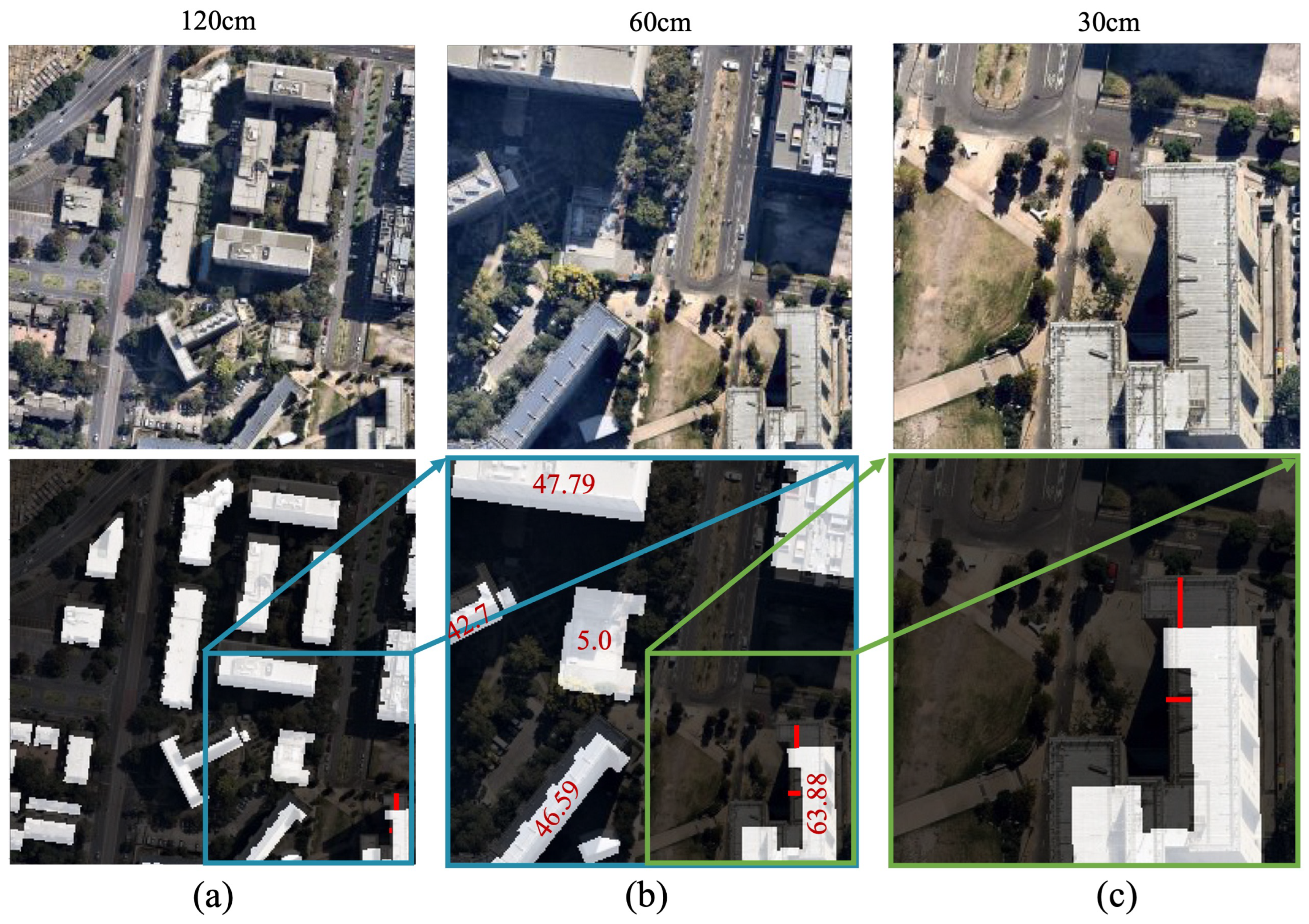
Figure 1, when spatial resolution rises from 120 cm/px (cm/px = centimeter per pixel, a unit of ground sample distance) to 60 cm/px, each original pixel is replaced by four smaller pixels, effectively quadrupling the displacement error. This label displacement error results in inaccurate training datasets, ultimately compromising the accuracy of building extraction models trained on these misaligned labels. Given its impact on large-scale data products, this problem has gained increasing attention, including research efforts such as the SpaceNet 4 Challenge [11]).
Tackling the misalignment problem is ongoing research, and the problem has recently devised many methods. Relief displacement correction [12], multitask learning [13], multilabel learning [14], and learning from depth [15] are studied as potential solutions. The segmented outputs in these methods are improved with several post-processing steps, including morphological operations that limit their robustness and end-to-end usage. Apart from addressing the misalignment problem, some studies distinguish between the facade and roof in a multi-view oblique image [16,17,18]. Wang et al. [19] developed the BONAI building dataset with labels for the roof, footprints, and the offset between them and employed a learning offset vector (LOFT) method with CNN that learned from the offset. The accuracy of the BONAI dataset was further improved recently by [14] using multilabel learning of footprint, roof, and additional ‘shape’ labels. These methods have provided remarkable achievements in tackling the misalignment problem, given that the annotations (labels) are available for multiple features of oblique-view buildings. However, developing a dataset that constitutes these features (footprint, roof, facade, and offset) is an additional challenge to the already difficult process of labeling footprints alone on the limited remote sensing images. While these methods require multiple post-processing steps or additional annotations for other building features over oblique-view images, other studies focus on knowledge distillation with a teacher–student learning approach.
Knowledge distillation (KD) [20] is a technique where a teacher model, trained on a large dataset, transfers its knowledge to a student model, which is typically smaller and more efficient. KD has been widely applied in learning from noisy labels (aka. supervision from label noise) [21,22] and has shown potential in remote sensing applications [23]. Xu et al. [24] adopted this KD-based teacher–student learning approach to address the label displacement problem. Their approach involved training a teacher on a large but noisy dataset (with misaligned labels) and distilling its knowledge into a student that learns from a smaller, cleaner dataset (without misalignment), making the student more robust to label noise. They compare their results to deep mutual learning (DML) [25], where multiple student models collaborate and teach each other while distilling knowledge from the teacher. Expanding on their work, Ref. [26] introduced fine-tuning learning (FTL), where models trained on noisy off-nadir images are adapted to true orthophotos, demonstrating that FTL was more effective than KD for training misalignment-tolerant students. Originally, KD was designed to transfer knowledge from large, high-performing models to smaller, deployable students [20], but this process inherently limits the student’s ability to surpass the teacher’s performance since smaller models retain less information. This constraint reduces accuracy in segmenting complex urban buildings, whereas FTL, unlike KD and DML, allows re-training beyond the pre-trained teacher’s limitations, enabling the student to develop greater noise tolerance and adapt more effectively to new datasets.
FTL adopts a pre-trained model on a source domain by further training it on a target domain using labeled target data while retaining knowledge from the source. FTL can also be called supervised domain adaptation if it explicitly addresses domain shifts between the source and target. Given that our datasets contain labels in both domains, FTL is more suitable than unsupervised domain adaptation (UDA) to adapt a student model to the target dataset. Studies have shown that FTL enhances building extraction accuracy [27,28] and is effective in fine-tuning models trained on large–noisy datasets for improved performance on small–clean datasets [29,30,31].
With FTL showing promising results in training misalignment-tolerant students compared with other teacher–student learning methods like KD, several research questions remain unanswered. These methods are introduced to address the misalignment problem, yet their experimentation in varied settings remains minimal. From the available studies of [24,26], two knowledge gaps are identified: (i) the teacher–student learning methods have not yet been studied for different building types of varying heights and images of different spatial resolutions; (ii) the available CNNs and EDNs are not benchmarked to identify the optimal teachers (large immovable networks) and students (lightweight and deployable) for the three methods.
To develop accurate building extraction models that are more tolerant to misalignment in off-nadir images and to investigate the two identified knowledge gaps, this study makes the following contributions:
  • FTL is introduced to mitigate misalignment between building image–label pairs caused by off-nadir angles. FTL is implemented within a teacher–student learning framework, where a large teacher model is pre-trained on a misaligned dataset (source domain) and subsequently fine-tuned on a smaller, error-free student dataset (target domain) to improve segmentation accuracy.
  • A structured experimental setup is designed to systematically compare FTL against KD, DML, and the models without FTL. Three new urban building datasets, including high-rise and skyscraper buildings, are developed with “large–noisy” and “small–clean” image–label pairs. The datasets and codes are openly released for reproducibility (see the data availability statement).
  • The methods are evaluated across four building types (low-rise, mid-rise, high-rise, and skyscrapers) and three spatial resolutions, ensuring a comprehensive performance analysis.
  • A comparative analysis of 43 representative lightweight CNNs, five optimizers, nine loss functions, and seven EDNs is conducted to identify the optimal trade-off between lightweight efficiency and high-performance models. The CNNs include state-of-the-art lightweight architectures from Google, Apple, Meta, Amazon, and Huawei. To the best of our knowledge, such a comprehensive benchmark of lightweight CNNs and their integration into an EDN is novel for building extraction.

2. Materials and Methods

The proposed method of FTL between large-noisy and small–clean datasets to achieve misalignment-tolerant models is carried out in a four-step workflow: (i) data preparation, (ii) selection of teacher and student network architectures, (iii) fine-tuning-based transfer learning, and (iv) evaluation of the fine-tuned students against the students distilled from KD and DML. The workflow is illustrated in Figure 2 and is detailed stepwise in this section.

2.1. Data Preparation

This study uses four datasets: one benchmark dataset for benchmarking the hyperparameters, CNNs, and EDNs for our experimental setup of FTL and three newly developed datasets for training, fine-tuning/distillation, and evaluation of EDNs. The benchmark dataset helps identify optimal configurations for setting up the teacher (pre-trained network) and students (fine-tuned/distilled networks) in FTL. Once configured, the teacher model is trained and evaluated on the teacher’s dataset (T), while the student models undergo fine-tuning/distillation and are evaluated using the student’s dataset (S) and Evaluation dataset ( E v ). The effectiveness of the student models in reducing misalignment is assessed based on their performance on these two datasets.
The benchmark dataset is derived from the widely used Massachusetts Building dataset [32]. A smaller subset of the dataset, as provided in [5], is used for experimental consistency and lower memory usage to benchmark the lightweight models. This subset crops the original 1500 × 1500 px (px = number of pixels) tiles to 256 × 256 px, and the training and test images are reduced by 4× and 2×. The number of validation images is kept the same as in the original dataset.
The teacher’s dataset (T) is developed by masking and tiling the building roof polygons provided by the City of Melbourne. See https://data.melbourne.vic.gov.au/explore/dataset/2020-building-footprints/information/ (accessed on 15 April 2024), 2020 Building Footprints from the City of Melbourne. Multi-resolution image tiles of 30, 60, and 120 cm/px spatial resolution are collected from the Nearmap Tile API. The vector labels are rasterized with reference to the image using Algorithm 1. The misalignment between these image–label pairs is not accounted for, making it the “large–noisy” teacher’s dataset.
Algorithm 1 Building Dataset Preparation from Nearmap API Service
Require: Building Geodatabase (GDB), API key, zoom level
Ensure: Geospatial tiles and rasterised building polygons
  1:
function FetchAndRasteriseTiles( p o l y g o n s , a p i K e y , z o o m )
  2:
     e x i s t i n g T i l e s
  3:
    for all  p o l y g o n p o l y g o n s  do
  4:
         c e n t r o i d CalculateCentroid( p o l y g o n )
  5:
         t i l e ConvertToTile( c e n t r o i d , z o o m )
  6:
        if  t i l e e x i s t i n g T i l e s  then
  7:
            i m a g e FetchTile( t i l e , a p i K e y )
  8:
           SaveTile( i m a g e )
  9:
            e x i s t i n g T i l e s e x i s t i n g T i l e s { t i l e }
10:
        end if
11:
    end for
12:
end function
13:
procedure DatasetPreparation( b u i l i n g G D B , a p i K e y , z o o m )
14:
     p o l y g o n s LoadShapefile( b u i l d i n g G D B )
15:
    FetchAndRasteriseTiles( p o l y g o n s , a p i K e y , z o o m )
16:
end procedure
17:
DatasetPreparation( b u i l d i n g G D B , a p i K e y , z o o m )
Student’s dataset (S) is developed for fine-tuning/distillation purposes by collecting images over the central business district (CBD) of Melbourne. The CBD consists mostly of high-rise and skyscraper buildings with complex structures, providing challenging urban environments. For the images, both off-nadir images and true orthophotos are collected from Nearmap. The orthophoto is separately downloaded and tiled, and the off-nadir image tiles are collected from the API service. City of Melbourne’s building roof polygons are overlaid over the true orthophoto image, and for the off-nadir image tiles, the buildings are manually annotated (by hand). Therefore, unlike T, this dataset provides ’clean’ image–label pairs.
The evaluation dataset ( E v ) is curated as a dataset to evaluate the fine-tuned/distilled networks on the manually annotated labels for image scenes of the four building types. This dataset does not have training samples (only validation). A subset of 55 image tiles of T is taken and manually annotated (by hand). The building types are separated according to their heights as defined by the Australian Bureau of Statistics (ABS). See: https://www.abs.gov.au/ausstats/abs@.nsf/Lookup/8752.0Feature+Article1Dec%202018 (accessed on 15 April 2024), Characteristics of Apartment Building Heights by ABS.
Table 1 summarizes the datasets, where (i) T contains misaligned image–label pairs for training and validation, (ii) S includes both off-nadir and true orthophoto images with clean labels, and (iii) E v features off-nadir images from T with clean labels. “Clean labels” refer to overlaying labels without misalignment. Both S and E v consist of complex high-rise buildings from the CBD, making them valuable for evaluating segmentation performance under challenging conditions. All datasets have an image size of 256 × 256 px. Figure 3 presents the study area and dataset samples.

2.2. Selection of Representative Teacher and Student Networks

EDNs enable flexible integration of backbone CNNs (encoders) for multi-scale feature extraction in semantic segmentation, with U-Net being a widely used architecture for building segmentation [5]. The encoder processes input images, while the decoder upsamples learned features to generate the segmented output, with skip connections preserving spatial details. An illustrative example of a U-Net EDN and two CNN examples—EfficientNetv2 and MobileViT—are provided in Figure 4.
EfficientNetv2 [33] is a lightweight CNN from Google Brain. It uses Fused-MBConv convolutional blocks alongside the NAS component, and like its predecessor v1, it offers multiple scaled versions. The network uses different variations of Mobile Inverted Bottleneck Convolution (MBConv) blocks: MBConv1, MBConv4, and MBConv6. These blocks are a type of inverted residual block central to the network architecture, providing efficient and flexible building blocks for CNNs. The blocks consist of the EdgeResidual layer to improve the flow of gradients during backpropagation, the non-linear activation function SiLU to introduce non-linearity, and the Squeeze-and-Excitation layer to improve the representational power of a network by explicitly modeling the interdependencies between the channels of convolutional features.
MobileViT [34] is a compact vision transformer developed for mobile devices. These models use MobileNetv2 (MV2) blocks to leverage their efficiency and lightweight nature for mobile and edge devices. MV2 blocks consist of an expansion layer, depthwise convolution, ReLU6 activation for non-linearity, pointwise convolution to project features back to the desired output dimension, and residual connection between input and output. It uses an additional MobileViT block, which is specialized to integrate the strengths of CNNs and transformers. It consists of the convolutional layer that extracts local features, the Transformer layer to capture global context and long-range dependencies, and the Reconstruction layer that reshapes and passes the output of the Transformer layer through another convolutional layer (to combine the local and global information). MobileViT is available in several smaller versions (s, xs, and xxs).
Optimal performance in EDNs is achieved by tuning hyperparameters, including the loss function ( L ), which quantifies prediction errors (e.g., dice loss, Jaccard loss), the optimizer (e.g., Adam, SGD) for weight updates, the learning rate ( η ) controlling step size during training, and the batch size, affecting memory use and convergence stability. The best-performing model is selected by systematically searching for hyperparameter configurations, training until validation loss stabilizes, and evaluating metrics like IoU and F1 score to ensure high segmentation accuracy and generalization. Therefore, before applying the proposed FTL and comparing it to other transfer learning methods, we carry out a systematic search of the (i) hyperparameters, (ii) EDNs, (iii) student models, and (iv) teacher models with an extensive benchmark study. The detailed benchmark is provided in Appendix A; however, its summary can be categorized into four steps:
Step 1.
Hyperparameter search: A CNN encoder (MobileOne-s1) is randomly chosen and integrated into a U-Net EDN to explore various hyperparameters, including learning rate, converging epoch, loss functions, and optimizers. Five optimizers and nine loss functions are tested, with learning rate scheduling and early stopping at the converging epoch. A combination of the RMSProp optimizer, dice loss, and 0.0001 learning rate provided the highest scores in most experiments.
Step 2.
EDN Comparison: The best hyperparameters from Step 1 are applied to eight state-of-the-art EDNs—U-Net, U-Net++ [35], U-Net3+ [36], LinkNet [37], PSPNet [38], FPN [39], DeepLabv3+ [40], and MANet [
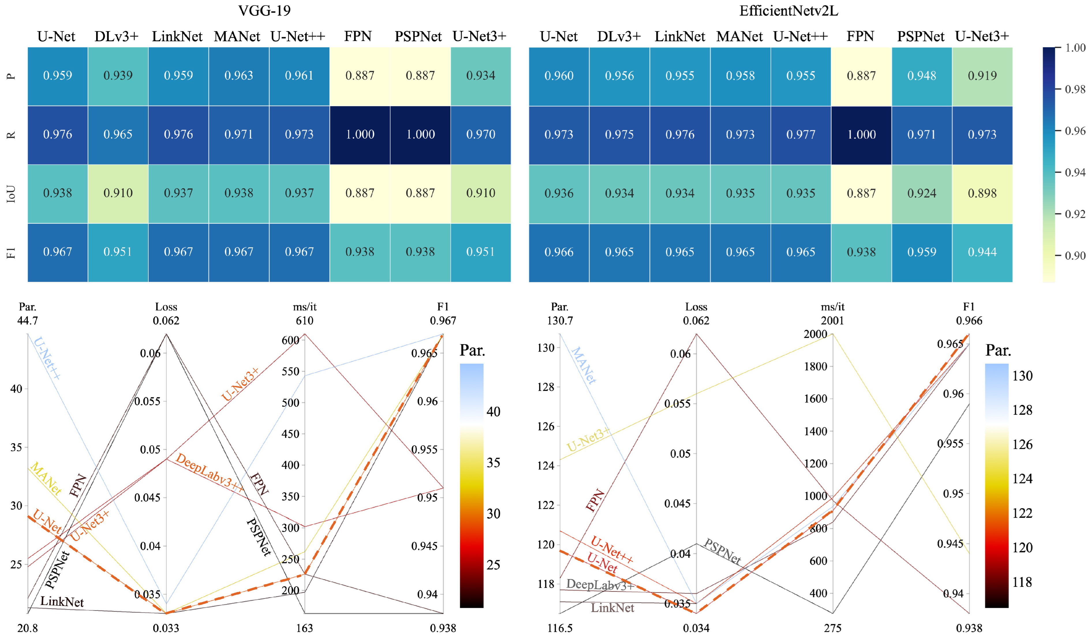
41]—to identify an architecture that balances model size and performance for the teacher and student networks. From the benchmarks, U-Net provided the best trade-off between the number of parameters, network complexity, and evaluation scores. It is therefore the best EDN to configure student and teacher models for the proposed FTL.
Step 3.
Student search: 43 lightweight CNNs (e.g., ResNeSt, GERNet, MobileOne, TinyNet, MobileViT, MobileNet, EfficientNet) (The explanation of the CNN along with their references is provided at 
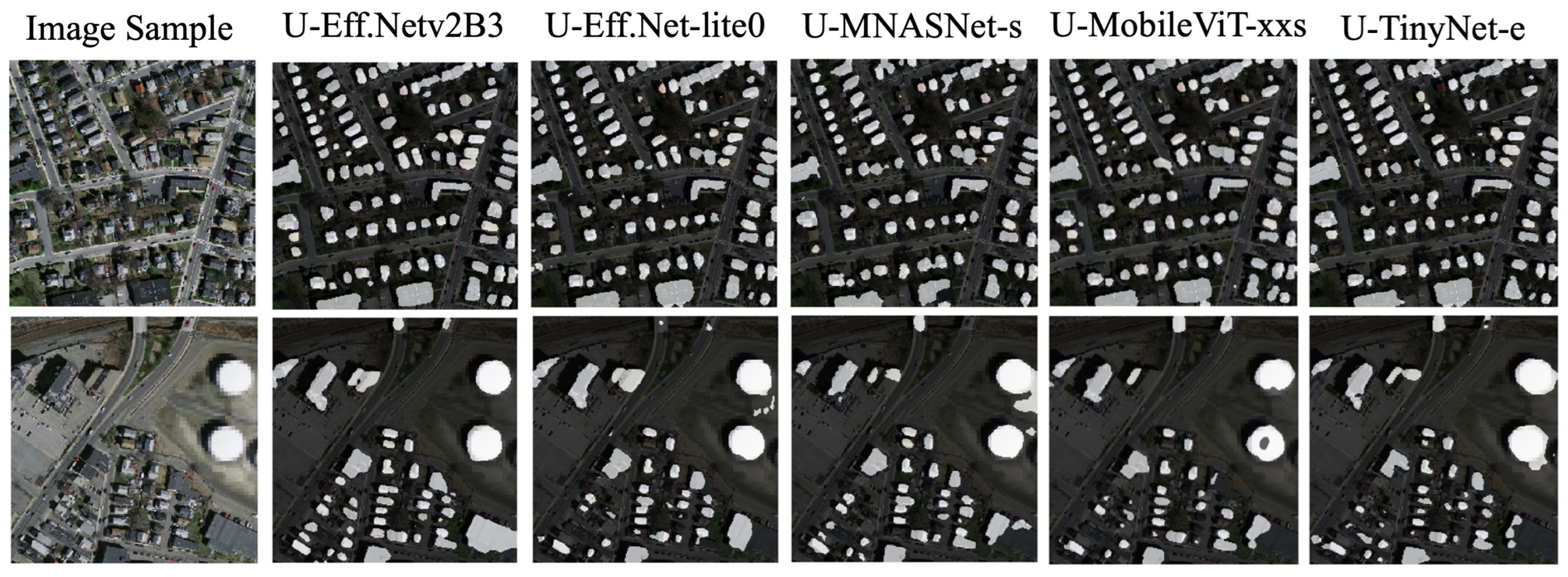
https://github.com/bipulneupane/TeacherStudentBuildingExtractor (accessed on 30 March 2025)). They are benchmarked as potential students. These CNNs are integrated into the EDN from Step 2 (U-Net) and trained with the hyperparameters from Step 1. For the integration, we remove their final layers of 1x1 convolution and fully connected layers. The remaining layers are then connected to the decoder that comprises 2D convolution, batch normalization (BN), ReLU, and attention layers. The top five best student models are selected based on a trade-off between network parameters, loss, training time, and evaluation scores. The top five student models were U-EfficientNetv2B3 (high scorer), U-EfficientNet-lite0 (best trade-off between evaluation scores and network parameters), U-MNASNet-s, U-TinyNet-e, and U-MobileViT-xxs (with the smallest size, suitable to configure student models).
Step 4.
Teacher search: For FTL, the teacher and student share the same EDN. However, to facilitate KD and DML for comparison, the teacher is a larger, static model distilling knowledge to smaller students. We evaluate a larger version of the student’s CNN and U-VGG19, given its strong benchmark performance [5]. U-VGG19 was identified as the best teacher with the highest F1 score and lower network parameters when compared with U-EfficientNetv2L (the largest version of the high-scorer EfficientNetv2B3 from Step 3).

2.3. Proposed Fine-Tuning-Based Transfer Learning (FTL)

The proposed FTL fine-tunes a model pre-trained on a source dataset by updating all layers on a target dataset. The process begins with pre-training an EDN on a large–noisy dataset, T (source domain = teacher’s dataset), containing misaligned labels. The model, denoted as f θ , learns broad feature representations. The pre-trained model (teacher) is then fine-tuned on a clean dataset S (target domain = student’s dataset). The goal is to adapt the model beyond the constraints of the teacher while retaining generalizable features learned from T. Fine-tuning consists of two key phases:

2.3.1. Pre-Training on Noisy Labels

The EDN, parameterised by θ , is trained on the noisy T dataset:
T = ( x T i , y T i ) i = 1 N T ,
where x T i R H × W × C represents the input image of height H, width W, and number of channels C. Similarly, y T i { 0 , 1 } H × W is the corresponding noisy building label, and N T is the number of samples in T. The training minimizes a segmentation loss, such as dice loss:
L Dice ( f θ ( x ) , y ) = 1 2 f θ ( x ) · y + ϵ f θ ( x ) + y + ϵ
where f θ ( x ) is the predicted segmentation mask, y is the input label mask, and ϵ prevents division by zero. The pre-training loss across T is
L T ( θ ) = 1 N T i = 1 N T L Dice ( f θ ( x T i ) , y T i )
After minimizing L T , we obtain the pre-trained model parameters, θ T .

2.3.2. Fine-Tuning on Clean Labels

The pre-trained model is fine-tuned on the student dataset:
S = ( x S j , y S j ) j = 1 N S ,
where x S j R H × W × C is the clean input image, y S j { 0 , 1 } H × W is its input label, and N S is the number of samples in S. Fine-tuning minimizes dice loss over S:
L S ( θ ) = 1 N S j = 1 N S L Dice ( f θ ( x S j ) , y S j )
The model parameters are updated using gradient descent:
θ S = θ T η θ L S ( θ )
where θ S are the fine-tuned parameters, η is the learning rate, and θ L S is the gradient of the loss. Since all layers are fine-tuned, the encoder and decoder adapt to S, improving segmentation precision.

2.4. Comparison Methods

The proposed FTL method is compared with existing teacher–student learning methods: knowledge distillation (KD) and deep mutual learning (DML). KD [20] distills a student on a small–clean dataset while being supervised by a teacher trained on a large–noisy set. DML [25] extends this by enabling multiple students to collaboratively learn from each other under teacher supervision. The two methods are established for the other applications of supervision from label noise [21,22,42,43]. Xu et al. [24] applied both methods to the label displacement problem we address, though with limited accuracy and unresolved knowledge gaps mentioned before. As KD and DML are the only teacher–student approaches introduced for this problem, we adopt them in our experimental setup with their respective loss functions for a fair, state-of-the-art comparison with FTL.

2.4.1. Knowledge Distillation

KD transfers knowledge from a large teacher model trained on noisy data (T) to a smaller student model trained on clean data (S) while minimizing performance loss. The student is optimized using a total loss:
L Total = α L Dice + ( 1 α ) L Distil
where α balances segmentation accuracy ( L Dice ) and feature alignment ( L Distil ). The distillation loss aligns multi-scale feature maps:
L Distil = L MSE σ p j t / τ , σ p j s / τ
where p j t and p j s are the predictions from the teacher and student for pixel j, σ is the sigmoid activation, and τ controls the softness of the predictions. The Mean Squared Error (MSE) loss is
L MSE = 1 N i = 1 N y j p j 2
where y j and p j are the GT and prediction for pixel j, and 1 N normalises the loss.
By optimizing L Total , KD ensures that the student retains the teacher’s knowledge while refining its segmentation accuracy. However, the student model is inherently constrained by the teacher’s performance, limiting its potential.

2.4.2. Deep Mutual Learning

DML enables multiple models to learn collaboratively rather than through a one-way teacher-to-student transfer. In this setup, one teacher and two students train jointly, benefiting from label supervision and mutual distillation. This encourages knowledge exchange, likely enhancing generalization and robustness, particularly in data-scarce settings like S.
Each model M k (teacher or student) is trained with a segmentation loss and a mutual distillation loss:
L Total ( k ) = α L Dice ( k ) + 1 α K i = 1 , i k K L Distil ( k , i )
where L Dice ( k ) is the segmentation loss for M k , L Distil ( k , i ) is the mutual distillation loss between M k and M i , and α balances segmentation accuracy and mutual learning.
The mutual distillation loss encourages agreement between models:
L Distil ( k , i ) = L MSE σ p j k / τ , σ p j i / τ
where p j k and p j i are the predictions for pixel j from models M k and M i , σ is the sigmoid activation function, and τ controls distribution softening.
By aligning their predictions, students develop a consensus on segmentation accuracy, improving generalization. DML is particularly effective when labeled data in S is limited, as models benefit from mutual knowledge exchange.

2.5. Experimental Setup

The experimental setup with training details, accuracy metrics, train-val settings, and baseline scores for comparison is provided below.

2.5.1. Training Details and Accuracy Metrics

All networks are wrapped in the PyTorch (version 2.2.2) using the Segmentation Models Pytorch library (version 0.3.4) [44] and trained on an Nvidia A100 GPU (Nvidia, Santa Clara, CA, USA) (with 80 GB RAM). The teacher and students are trained up to 50 and 200 epochs, respectively. The learning rate is reduced upon a plateau of intersection over union (IoU) metric by a factor of 0.1 with a patience of 10 epochs. A sigmoid function classifies the final binary outputs. Four accuracy metrics are used for evaluation: precision (P), recall (R), IoU, and F1 score. The mathematical notation of the metrics is from [5].

2.5.2. Train-Val Settings

The experiments are performed in different experimental settings for FTL, KD, and DML. Depending on the training (train) and validation (val) subsets of T, S, and Ev datasets, five experimental settings are used for the comparison:
  • T–T: training/fine-tuning/distilling on T; validation on T.
  • S–S: training/fine-tuning/distilling on S; validation on S.
  • T–S: training/fine-tuning/distilling on T; validation on S.
  • T–Ev: training/fine-tuning/distilling on T; validation on Ev.
  • S–Ev: training/fine-tuning/distilling on S; validation on Ev.

2.5.3. Baseline Scores for Comparison

With the teacher and students identified from the benchmarks, we trained them on the T and S datasets alone. The trained models were evaluated on Ev to produce the baseline scores for the comparison of the transfer learning methods.
Teacher’s baseline scores were produced in T–T, T–S, and T–Ev settings, as reported in Table 2. From the difference in T–T and T–S settings, it was found that the teacher’s ability to generalize the validation samples from S was influenced by the domain shift between T and S. This domain shift can be attributed to two primary factors: the presence of unfamiliar, complex urban high-rise buildings in S and the contrast between the precision of ortho-rectification between the samples of T and S. However, in the T–Ev setting, the teacher demonstrated its capacity to generalize complex high-rise buildings in Ev, even though it was trained on misaligned labels in T. The complexity of the clean data S and Ev was prominent in the experimental results.
Student’s baseline scores (without transfer learning) were studied in S–S and S–Ev settings. 
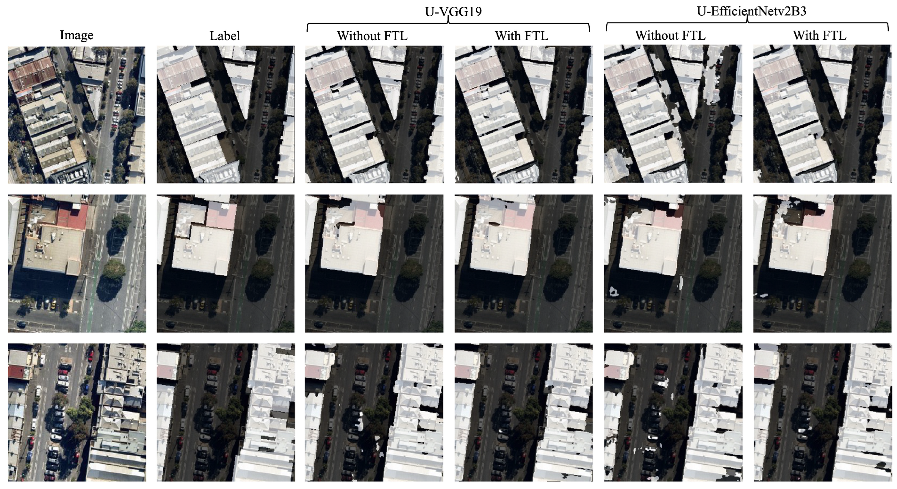
Table 3 reports their baseline scores along with the performance of the three knowledge transfer methods. U-VGG19 (0.893 F1) and U-EfficientNetv2B3 (0.819 F1) score the highest when validated on S and Ev, respectively. The performance of students after FTL and other knowledge transfer methods will be evaluated against these baseline scores.
Having thus established our experimental setup, we now present the comparative evaluation of FTL against KD and DML across different types of urban buildings.

3. Results

This section presents the results from the proposed FTL method and compares FTL with KD and DML. The individual performances are first reported for the three methods, and then the performance, training times, and computational efficiency are compared. In addition, an ablation of FTL vs. without FTL is reported at the end of this section.

3.1. Individual Performances of FTL, KD, and DML

First, the results from the proposed FTL method and the KD and DML comparison methods are presented individually.

3.1.1. Results from FTL

FTL consistently improved the performance of all student models, demonstrating its effectiveness over standalone training (baseline). The performance of FTL under S–S and S–Ev settings is reported in Table 4. In both S–S and S–Ev, all students achieved higher scores than their baseline counterparts (Table 3), except for U-EfficientNet-lite0 under S–Ev. For example, the IoU of U-EfficientNetv2b3 improved by 3.6% after FTL (0.805 vs. 0.769) in the S–S setting and by 4.4% (0.752 vs. 0.708) in the S–Ev setting. Additionally, all students trained with FTL outperformed the teacher model (T–S setting from Table 2) when evaluated on the S dataset, indicating that fine-tuning provided better adaptation to the target domain. For example, U-VGG19 after FTL provided 16.3% higher IoU (0.832 vs. 0.713) compared with the teacher’s baseline score (before FTL).
Among the students, U-VGG19 achieved the highest F1 score (0.903) in the S–S setting, while U-EfficientNetv2B3 performed best in the S–Ev setting (0.847 F1). This suggests that U-EfficientNetv2B3 is the most suitable student for FTL when generalizing to the Ev dataset, making it the preferred choice for enhanced segmentation performance in more complex environments.

3.1.2. Results from KD

The performance of KD under S–S and S–Ev settings is reported in Table 5. In comparison to the students’ baseline scores, most distilled networks (with KD) underperformed, including a decline in F1 scores. KD applied to U-VGG19 with self-distillation (same teacher and student model) showed some improvement in both S–S and S–Ev settings, but it still failed to surpass FTL and did not achieve model compression. U-MNASNet-s was the only exception, producing higher scores in S–Ev, indicating that certain architectures may benefit more from distillation than others.
Among the smaller student models, U-EfficientNetv2B3 achieved the highest F1 score (0.851) in the S–S setting, while U-EfficientNet-lite0 performed best in the S–Ev setting (0.784 F1). This suggests that U-EfficientNet-lite0 is the most effective student for KD in the Ev dataset, offering a significant reduction in network parameters—from 29.1 M (U-VGG19) to 5.6 M. This is an 82% decrease, demonstrating the potential of KD for lightweight model compression.

3.1.3. Results from DML

Similar to KD, experiments were conducted between the teacher (U-VGG19) and the selected students, with DML performed between six pairs of students. Due to the high computational cost of loading multiple EDNs into memory, only two students were distilled at a time. Notably, U-MobileViT-xxs was excluded from DML experiments due to its poor performance with KD.
The results under S–S and S–Ev settings are reported in Table 6. In the S–S, all students performed worse than their baseline scores, with most student pairs yielding lower scores. However, DML showed some improvement in the S–Ev, although it also reduced performance in at least one student from each pair. Two pairs, (U-VGG19, U-TinyNet-e) and (U-EfficientNetv2B3, U-MNASNet-s), showed improvements, with both students in each pair achieving higher F1 scores than their baseline models. The pair of (U-VGG19, U-EfficientNetv2B3) produced the highest average scores across both settings, suggesting that DML can benefit certain student pairs, but its impact is inconsistent and highly dependent on the models involved.

3.2. Comparison of FTL with Baseline, KD, and DML

After reporting the individual performances of FTL, KD, and DML, the three methods are compared in terms of performance, training time, and computational efficiency.

3.2.1. Performance Comparison

The performance of FTL against standalone models (baseline), KD, and DML is summarized for the two top-performing students in S–S and S–Ev settings: U-VGG19 and U-EfficientNetv2B3. The comparison, illustrated with radar charts in Figure 5, highlights that FTL consistently outperformed baseline scores and other transfer learning methods across both settings.
In the S–S setting, FTL with U-VGG19 achieved the highest F1 score of 0.903, followed by KD with U-VGG19 (0.901 F1). In the S–Ev setting, FTL with U-EfficientNetv2B3 obtained the highest F1 score of 0.847, followed by its standalone training (baseline) at 0.819 F1. KD provided a slight improvement over baseline scores with U-VGG19 as the student, but since it is a self-distillation, it did not offer any model compression. In contrast, KD with U-EfficientNetv2B3 provided a 50% reduction in network parameters (29.1 M vs. 14.6 M), but the performance trade-off was minimal (F1: 0.851 vs. 0.855 for KD vs. Baseline). Similarly, DML with U-EfficientNetv2B3 showed only a marginal difference from the baseline (F1: 0.832 vs. 0.855).
In the S–Ev setting, FTL remained the best-performing approach, outperforming the baseline and both KD and DML for U-VGG19 and U-EfficientNetv2B3. While all three methods outperformed baseline scores with U-VGG19, none provided model compression. With U-EfficientNetv2B3, KD led to a 4.5% F1 reduction (0.774 vs. 0.819), while DML resulted in a smaller 0.9% drop (0.810 vs. 0.819).
Overall, U-EfficientNetv2B3 was the best student for FTL, though it did not achieve model compression. KD and DML enabled compression but at the cost of reduced performance. U-EfficientNet-lite0 proved to be the best student for KD, reducing network parameters by 82% (from 29.1 M to 5.6 M) compared with the teacher (U-VGG19). With DML, only a few student pairs improved both models’ scores. These findings indicate that FTL is the most effective method for mitigating the impact of misaligned building labels, significantly outperforming KD and DML in both accuracy and consistency.

3.2.2. Analysis of Training Time and Computational Efficiency

The training times (ms/it) for different student models under FTL, standalone training, and KD are shown in Figure 6, while DML is excluded due to its training time dependence on the number and size of distilled students. KD incurred the highest training time across all models due to the additional overhead of aligning student predictions with the teacher’s soft labels, significantly increasing processing time per iteration. In contrast, standalone training was the fastest, as it trained models from scratch without prior knowledge transfer. FTL remained computationally efficient, achieving training times comparable to standalone training while leveraging pre-trained weights. The computational time could be reduced if fewer layers were unfrozen during the fine-tuning. The difference between standalone and FTL was minimal, as seen with U-TinyNet-e (181 ms/it in both) and U-MobileViT-xxs (294 ms in FTL vs. 296 ms in standalone), indicating fine-tuning introduced negligible overhead while retaining transfer learning benefits.
DML required significantly longer training times than all other methods, as shown in Table 6. The computational costs in DML increase based on the number of students and model sizes. Unlike KD and FTL, which involve only a single teacher–student relationship, DML’s complexity scaled quadratically (compared with the standalone training and FTL), making it the least efficient for applications where training time is a constraint. It also required more memory and GPU resources for training, as it had to load all students, the teacher, and the training data simultaneously.
Therefore, FTL is the most computationally efficient transfer learning method among the compared, maintaining near-standalone training speeds while benefiting from pre-trained models. KD incurred significant computational costs, while DML was the least efficient due to its model interactions. FTL offered the best balance between efficiency and transfer learning benefits, making it ideal for lightweight U-Net segmentation models in resource-constrained settings.

3.3. Ablation Study: With FTL vs. Without FTL

The performance gains from FTL compared with the baseline (without fine-tuning) are presented in Table 7, showing improvements in IoU and F1 scores across all students. FTL consistently improved IoU (up to 6.1%) and F1 scores (up to 4.2%) for all models in the Ev dataset. U-VGG19 and U-EfficientNetv2B3 produced the highest scores in S–S and S–Ev settings, respectively, showing the effectiveness of fine-tuning.
A visual comparison of segmentation outputs before and after FTL (Figure 7) further highlights the advantages of fine-tuning. FTL reduced over-segmentation and minimized outliers, leading to cleaner building extractions and improved alignment with input labels. These findings confirm that fine-tuning significantly improves segmentation accuracy compared with standalone training.

4. Discussion

This section further dissects the results from the previous section and provides a discussion on how the proposed method compares to KD and DML for different building heights and different spatial resolutions of remote sensing images. Furthermore, the limitations and opportunities are discussed.

4.1. Investigation of Different Building Heights

The effects of building heights were studied by separating the image scenes of Ev into four categories of building types: low-rise, mid-rise, high-rise, and skyscrapers. The chart in Figure 8 shows the performance of FTL as compared with the teacher, KD, and DML. FTL outperformed the teacher, KD, and DML, with the highest scores for low-rise (0.943 F1), mid-rise (0.868 F1), and skyscrapers (0.697 F1). Both student and teacher networks yielded F1 and average scores above 90% for low-rise buildings. The performance degraded with the increased height of the buildings.
A mean difference (MD) of the four performance scores (difference in ‘Avg.’ from Figure 8) is further examined to observe the clear differences between our FTL versus the teacher, KD, and DML. The MD is plotted in Figure 9. It indicates that FTL outperforms KD and DML across all building types, with the most significant improvements seen in mid-rise and skyscraper buildings. For low-rise structures, FTL showed only a marginal improvement (0.4–1.7%) over other methods, suggesting that fine-tuning was not impactful for simpler buildings. In mid-rise buildings, FTL provided a moderate gain over KD (2.8%) and a notable advantage over DML (5.8%), making it a better alternative in moderately complex urban settings. For high-rise buildings, the teacher performed better than the FTL (−4.6%), meaning fine-tuning did not enhance performance for these buildings. However, FTL still outperformed KD (2.8%) and DML (7.5%), confirming its effectiveness compared with KD and DML. The greatest improvements are seen in skyscrapers, where FTL significantly outperformed all methods, with gains over teacher (1.5%), KD (3.2%), and DML (3.4%), showing its robustness in handling extreme building heights and off-nadir distortions. These results suggest that FTL is most beneficial for complex urban environments, particularly for taller buildings.

4.2. Investigation of Different Spatial Resolutions

The study was further dissected in terms of the spatial resolution of the images. Figure 10 shows sample output from each method with images of three spatial resolutions for the four building types. For the low-rise buildings, FTL increased the generalization of the buildings in all three resolutions and achieved the highest F1 of 0.943. The green boxes highlight the network’s ability in instance segmentation of buildings. The blue boxes in the 30 cm/px images show that FTL could separate the roofs from the facades. KD and DML over-segmented the images. For mid-rise, the performance was lower than low-rise, with FTL showing some improvements. The blue boxes in the 60 cm/px image sample show FTL’s ability to segment out the facades and the gaps between the buildings. For the high-rise, the teacher performed with the highest evaluation scores despite the noisy training data. However, it was seen that FTL could separate roofs from the facades with better segmentation. For skyscrapers (outlined with orange boxes), the segmentation was poor. FTL produced the highest scores but with increased noise. The 30 cm/px sample in Figure 10 shows the segmentation of the tallest skyscraper in Melbourne (319 m high).
The spatial resolution of the images affected the segmentation of the four building types differently. From Figure 10, the students performed poorly on the highest resolution (30 cm/px) images. Low-rise buildings were too small to segment accurately, and high-rise buildings and skyscrapers were too large to fit into the image tiles. The best visual results were achieved at the resolution of 60 cm/px, except for skyscrapers, for which the lowest resolution of 120 cm/px provided the best segmentation.

4.3. Limitations and Opportunities

FTL proved most beneficial for complex urban environments as it outperformed other transfer learning methods. Figure 11 (sample on top) shows the considerably accurate segmentation output from the two best students using the FTL approach. The students could produce relatively precise building segments despite the presence of highly dense and connected buildings. Moreover, they also precisely segmented buildings with multiple roofs and smaller objects.
However, segmentation challenges arose in taller buildings (high-rises and skyscrapers) due to shadows, occluded buildings, reflections from glass facades, rooftop objects, and label misalignment. This limitation is shown in the bottom half of Figure 11, where even the top-performing models struggled to segment skyscrapers. While FTL reduced over-segmentation, further improvements could be achieved by integrating LiDAR or by learning multiple features of oblique-view images, such as footprints, roofs, and facades.
The limitations of the compared methods, KD and DML, were more than the inherent inability of student models to surpass the teacher. They were less effective in tackling the label displacement error, and implementing them required storing multiple networks in memory, posing deployment challenges. FTL was more memory-efficient and easier to integrate into operational systems. The limitation of FTL in terms of implementation is that it depends on a small but high-quality clean dataset, which may not always be available. Most benchmark datasets contain noise and label displacement errors [45]. This can lead to model overfitting, as observed in our benchmarks with FPN-VGG19, PSPNet-VGG19, and FPN-EfficientNetv2L. Expanding benchmarks is crucial to identifying the best trade-off between lightweight and high-performance models. Furthermore, FTL requires testing on diverse geographic datasets with varying architectural styles, climate conditions, and sensor data sources (e.g., New York, Tokyo, and rural areas) to assess its generalizability. Beyond building extraction, FTL could be adapted for flood damage assessment, post-earthquake building extraction, and other remote sensing applications in resource-constrained environments, enhancing its practical impact.

5. Conclusions

This study proposed fine-tuning-based transfer learning as an effective method for building extraction from remote sensing imagery, specifically addressing the misalignment problem (label displacement errors) caused by off-nadir images. Unlike the existing methods of KD and DML, which primarily focus on model compression, FTL leverages the teacher–student learning framework to fine-tune a pre-trained model on a smaller, high-quality dataset. This approach allows better adaptation to the target domain without compromising segmentation accuracy, making it a more robust alternative to the previous transfer learning methods.
A structured experimental framework was designed with three new urban building datasets that incorporate both large–noisy (misaligned) and small–clean (manually annotated) image–label pairs. This setup enabled a controlled evaluation of FTL, KD, and DML across different building types and spatial resolutions. Additionally, an extensive benchmark study was conducted, evaluating 43 representative lightweight CNNs, five optimizers, nine loss functions, and seven encoder–decoder networks (EDNs) to identify the optimal balance between lightweight efficiency and high segmentation accuracy. The benchmark found that U-VGG19 and U-EfficientNetv2B3 are the best (in terms of accuracy, training time, and model size) teacher and student models.
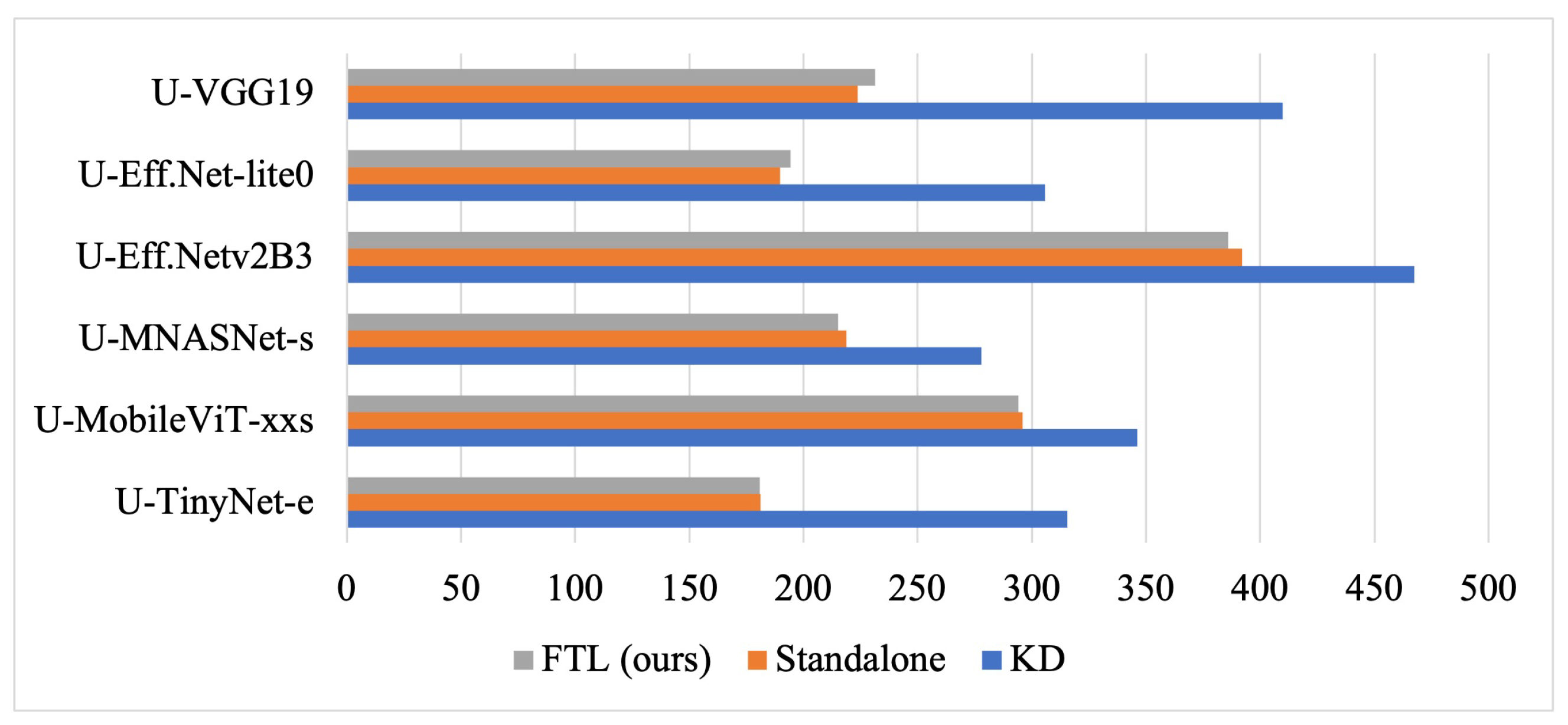
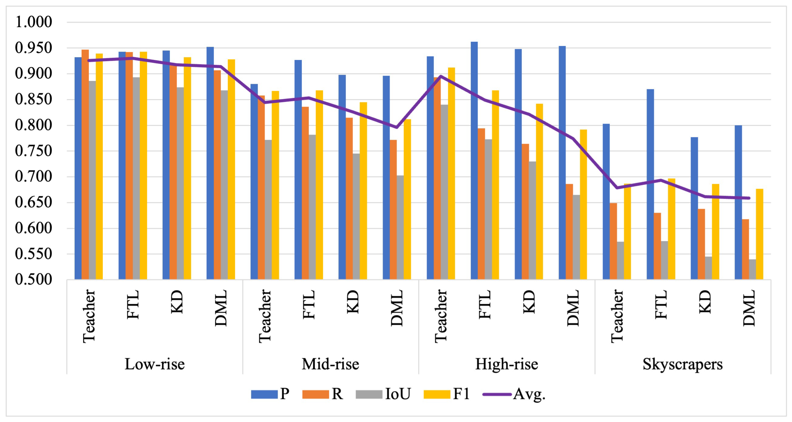
The results demonstrated that FTL consistently outperformed standalone training (baseline), KD, and DML, achieving higher F1 and IoU scores across different building types and spatial resolutions. Among the student models, U-VGG19 achieved the highest F1 (0.903) in the S–S setting, while U-EfficientNetv2B3 performed best in the S–Ev setting (0.847 F1), suggesting its suitability for generalizing to unseen datasets. KD and DML provided some improvements in model efficiency but at the cost of reduced segmentation accuracy. Additionally, FTL proved computationally efficient, introducing minimal overhead compared with standalone training, while KD incurred significant computational costs, and DML was the least efficient due to its quadratic increase in complexity when distilling multiple students.
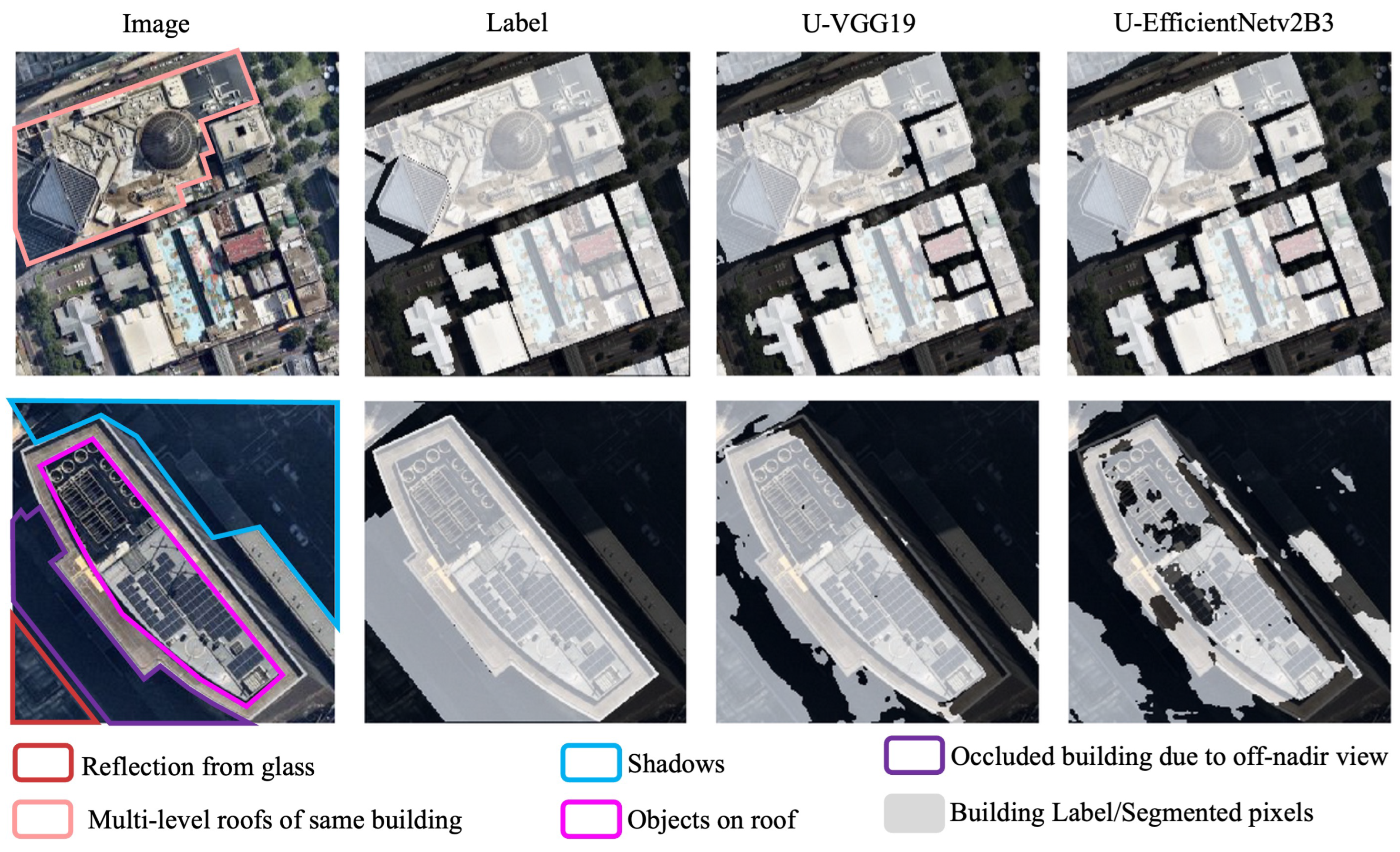
Further investigations revealed that FTL was particularly effective in complex urban environments, especially for skyscrapers, where it significantly outperformed KD and DML in handling off-nadir distortions and misaligned building labels. However, high-rise buildings remained challenging, with the teacher sometimes performing better than fine-tuned models. The analysis of spatial resolution further highlighted that 60 cm/px imagery provided the best balance for building extraction, and 120 cm/px images were more suitable for skyscrapers. The 30 cm/px images introduced intricate noise (over-segmentation and outliers) for small buildings as they were too small for accurate segmentation, and the high-rises and skyscrapers were too large to fit in a single image tile.
These findings highlight the potential of FTL as a robust method for accurate building extraction, particularly in off-nadir images of urban environments. The approach can be extended to other remote sensing applications, such as flood damage assessment, post-disaster building extraction, and large-scale urban monitoring, where accurate segmentation under variable conditions is needed. Future research could explore self-supervised learning to reduce reliance on clean labels, test FTL across diverse geographic regions, and investigate multi-feature learning for enhanced segmentation of oblique-view images.

Author Contributions

Conceptualization, B.N.; methodology, B.N.; software, B.N.; validation, B.N. and J.A.; formal analysis, B.N.; investigation, B.N.; resources, B.N.; data curation, B.N.; writing—original draft preparation, B.N.; writing—review and editing, B.N., J.A. and A.R.; visualization, B.N.; supervision, J.A. and A.R.; project administration, J.A.; funding acquisition, B.N. and J.A. All authors have read and agreed to the published version of the manuscript.

Funding

This research received no external funding.

Data Availability Statement

The codes to access and reproduce the datasets are available at: https://github.com/bipulneupane/TeacherStudentBuildingExtractor (accessed on 30 March 2025).

Acknowledgments

The first author (B.N.) is supported by the University of Melbourne for his PhD research and is awarded the Melbourne Research Scholarship. The experimental results were produced using the LIEF HPC-GPGPU Facility hosted at the University of Melbourne, which was established with the assistance of LIEF Grant LE170100200. The authors would like to thank Nearmap for providing the API service to collect the image data for the experiments.

Conflicts of Interest

The authors declare no conflicts of interest.

Appendix A. Benchmarking Network Architectures for Teacher and Student Models

Appendix A.1. Hyperparameter Search

The optimal hyperparameters were searched with a randomly selected MobileOne-s1 CNN encoder for U-Net EDN (abbr. U-MobileOne-s1). Then, using the loss function of total loss, five optimizers—Adam, stochastic gradient descent (SGD), RMSprop, Adadelta, and Nadam—were compared with find the optimizer that yields the highest evaluation scores. The total loss was formulated as the sum of dice loss and binary focal loss. The RMSProp optimizer produced the highest scores for our experimental settings with a trade-off between loss and faster-converging epochs. Then, using RMSProp, nine loss functions—binary cross entropy (BCE), BCE dice loss, BCE Jaccard loss, binary focal dice loss, binary focal Jaccard loss, Jaccard loss, dice loss, binary focal loss, and total loss—were further compared. A combination of RMSProp optimizer and dice loss yielded the highest scores, as shown in Table A1. Adam was marginally close to RMSProp optimizer. Jaccard loss produced the same IoU and F1 with a faster-converging epoch compared with dice loss but yielded a lower loss. The learning rate of 0.0001 produced the highest scores in most experiments. Therefore, the selected hyperparameters are RMSProp optimizer, dice loss, and 0.0001 learning rate.
Table A1. Hyperparameter search using a U-Net with randomly chosen lightweight CNN of MobileOne-s1. Five optimizers are tested with a total loss (dice loss + binary focal loss). The optimizer with the highest F1 score is then used to test the nine loss functions. Columns ‘ms/it’ (millisecond/iteration) and ‘Ep’ report training time and converging epoch. Boldface: best performance.
LossPRIoUF1ms/itEp.
Optimizers (with Total Loss)
Adam0.1770.9590.9630.9260.96037626
SGD0.3380.8890.9900.8820.93520028
RMSProp0.1770.9580.9640.9270.96129422
Adadelta0.4440.9270.7840.7440.84542029
Nadam0.1790.9570.9650.9270.96139520
Loss Functions (with RMSProp optimizer)
BCE0.2000.9500.9730.9270.96165826
BCE Dice0.2430.9490.9750.9280.96165815
BCE Jaccard0.2850.9460.9780.9270.96131214
Binary Focal Dice0.1910.9510.9660.9220.9583247
Binary Focal Jaccard0.2170.9550.9670.9260.96029226
Jaccard0.0720.9530.9720.9280.96228218
Dice0.0390.9480.9770.9280.96231420
Binary Focal0.1200.9750.8960.8760.93229230
Total Loss0.1770.9580.9640.9270.96129422

Appendix A.2. EDN Comparison

With the best hyperparameters found, we further used the U-MobileOne-s1 with RMSProp optimizer and dice loss to investigate the other EDNs. The results are shown in the first half of Table A2. Results indicated that U-Net++ achieves the highest scores (0.964 F1), closely followed by U-Net, which offered faster training and lower network parameters. Compared with U-Net++, U-Net provided the best trade-off between network parameters (9.1 M vs. 12.3 M) and evaluation scores with a marginally lower F1 of 0.962 and less complexity in network architecture. Opting for U-Net’s slightly lower evaluation scores, we prioritized lower parameters and faster training for small deployable students. Fewer parameters mean a smaller model size and faster training time, which is essential for students in knowledge transfer. Among the other EDNs, MANet matched U-Net in IoU and F1 but with nearly 6x more parameters. LinkNet and DeepLabv3+ were lightweight but yielded lower scores. FPN and PSPNet, despite faster training, overfit on the dataset. U-Net is, therefore, the best EDN configuration for students.
Table A2. Search of EDN and CNN encoders for student networks. Eight EDNs are first tested with a randomly chosen MobileOne-s1 CNN to identify the EDN with the best trade-off between network parameters and evaluation scores. The best performance scores among the EDNs are highlighted in bold. This EDN is then used to test and benchmark the 43 identified lightweight CNNs. Network parameters (Par.) are shown in Millions. The top three scores for the lightweight CNNs are underlined and ranked in order from one to three with a postscript.
Par.LossPRIoUF1ms/it
EDN with MobileOne-s1 encoder
U-Net9.10.0390.9480.9770.9280.962314
DeepLabv3+5.70.0440.9370.9790.9190.956287
LinkNet6.20.0420.9450.9730.9220.958326
MANet53.30.0390.9480.9760.9280.961376
U-Net++12.30.0360.9540.9750.9330.964395
FPN5.70.0620.8871.0000.8870.938309
PSPNet3.80.0620.8871.0000.8870.938168
U-Net (best trade-off of Par. and F1) with lightweight CNNs as encoder
ResNet-1814.30.0380.9490.97730.9290.962109
DenseNet-12113.60.03730.9500.97730.93130.9633629
SE-ResNet-1814.40.0390.9500.9740.9270.9611511
MobileNet-v26.60.0390.9510.9720.9270.961201
MobileNetv3-s3.60.0440.9400.9740.9180.956281
MobileNetv3-l6.70.0430.9460.9700.9210.957316
Eff.NetB06.30.0380.95230.9730.9290.962304
Eff.NetB18.80.0380.9500.9760.9300.962461
Eff.NetB210.00.03730.95610.9710.93130.9633459
Eff.NetB313.20.03730.9510.97730.9300.9633485
Eff.Net-lite05.60.0390.9500.9740.9280.962187
Eff.Net-lite16.40.0390.9480.9760.9280.961233
Eff.Net-lite27.20.0390.9480.9750.9270.961229
Eff.Net-lite39.40.0380.9480.97820.9290.962258
Eff.Net-lite414.40.0400.9450.97820.9260.960313
Eff.Netv2B07.60.0380.9510.9750.9290.962284
Eff.Netv2B18.60.03730.95320.9750.93130.9633334
Eff.Netv2B210.40.03730.9510.97730.93130.9633347
Eff.Netv2B314.60.03510.95610.9750.93410.9651408
SK-ResNet-1814.60.0380.9480.97820.9290.962201
DPN-6817.00.0410.9450.9750.9240.959493
ResNeSt-1417.60.03620.95230.97730.93220.96421592
GERNet-s12.80.0400.9470.9740.9250.9601803
MobileOne-s08.60.0380.9480.97910.9300.963610
MobileOne-s19.10.0390.9500.9750.9280.962287
MobileOne-s213.60.0390.9490.9750.9280.961296
MobileOne-s316.20.0390.9500.9730.9270.961293
HRNet-1816.10.0380.95230.9740.9290.962870
MNASNet-s2.210.0430.9380.97820.9200.957214
MobileViT-s8.00.0400.9460.9750.9250.960289
MobileViT-xs4.30.0400.9470.9750.9260.960294
MobileViT-xxs3.130.0420.9430.9750.9220.958299
FBNet-c1005.20.0410.9470.9730.9240.959229
FBNet-v3b8.60.0420.9430.9740.9210.958690
FBNet-v3d10.30.0410.9430.97820.9250.960769
FBNet-v3g16.80.0400.9450.9760.9250.960917
HardCoRe-NAS-a6.50.0420.9400.97910.9220.958283
HardCoRe-NAS-f9.40.0430.9370.9800.9200.957552
MixNet-s4.30.0440.9430.9700.9180.956429
MixNet-m5.20.0430.9430.9740.9210.957498
MixNet-l7.60.0410.9480.9720.9240.959532
TinyNet-a6.70.0420.9440.9750.9230.959296
TinyNet-e2.320.0450.9340.97910.9160.955182

Appendix A.3. Student Search

After identifying U-Net as the best-performing EDN, 43 representative lightweight CNNs identified from the computer vision domain were integrated into U-Net for the student search. Thus developed U-Net configurations of the 43 CNNs are shown in the second half of Table A2. The high scorer was U-EfficientNetv2B3 (0.965 F1), U-EfficientNet-lite0 provided the best trade-off between evaluation scores and network parameters, and the lightest students were U-MNASNet-s (2.2M), U-TinyNet-e (2.3M), and U-MobileViT-xxs (3.1M). These EDNs were, therefore, selected as the top five students for the rest of the study. Figure A1 shows the segmentation outputs from these five students on two random samples from the validation subset of the Massachusetts building dataset. The trend showed that the segmentation performance decreases with the number of network parameters.
Figure A1. Segmentation results of the selected lightweight students on the subset of Massachusetts building dataset. U-EfficientNetv2B3 produced the highest F1 score of 0.965. Other students produced lower scores but with trade-offs between network parameters, training time, loss, and evaluation scores as seen in Table A2.
Remotesensing 17 01251 g0a1

Appendix A.4. Teacher Search

For FTL, the teacher and student constitute the same EDN network. For KD and DML, the best teacher was identified from the comparison of VGG19 (top scorer from [5]) and EfficientNetv2L (largest version of the best-performing CNN of EfficientNetv2B3) with eight EDNs. The heatmaps and the parallel coordinate plots in Figure A2 provide minute details to identify the most optimal trade-off from the networks. With VGG-19, three EDNs of U-Net, LinkNet, and U-Net++ achieved the highest average of the four accuracy metrics (0.960) and an F1 of 0.967. However, with EfficientNetv2L, only U-Net yielded the highest F1 score, higher than DeepLabv3+, LinkNet, MANet, and U-Net++. FPN and PSPNet provided overfitting results (with recall up to 1.000). LinkNet provided the best trade-off with VGG-19, while U-Net provided that with the highest F1 and lower parameters with both CNNs. Therefore, U-VGG19 is the teacher for our transfer learning study.
Figure A2. Teacher search with VGG-19 (left) and EfficientNetv2B3 (right) as CNNs for the state-of-the-art EDNs. The heat maps on top compare the evaluation scores of the EDNs. The parallel coordinate plots on the bottom show the trade-off between network parameters (Par.), loss, training time (ms/it), and F1 score. The network with the dashed line (U-Net) provides the best trade-off among the variables.
Remotesensing 17 01251 g0a2

References

  1. Chauhan, A.; Wasim, M.; Mohanty, S.; Pandey, P.C.; Pandey, M.; Maurya, N.K.; Rankavat, S.; Dubey, S.B. Earth observation applications for urban mapping and monitoring: Research prospects, opportunities and challenges. Earth Obs. Urban Monit. 2024, 197–229. [Google Scholar] [CrossRef]
  2. Camacho, R.; Aryal, J.; Rajabifard, A. How do disasters disrupt the spatial growth of informal settlements? A multi-temporal remote sensing approach–The case study of Mocoa, Colombia. Habitat Int. 2025, 156, 103272. [Google Scholar]
  3. Herfort, B.; Lautenbach, S.; Porto de Albuquerque, J.; Anderson, J.; Zipf, A. The evolution of humanitarian mapping within the OpenStreetMap community. Sci. Rep. 2021, 11, 3037. [Google Scholar]
  4. Li, J.; Huang, X.; Tu, L.; Zhang, T.; Wang, L. A review of building detection from very high resolution optical remote sensing images. Gisci. Remote Sens. 2022, 59, 1199–1225. [Google Scholar]
  5. Neupane, B.; Aryal, J.; Rajabifard, A. CNNs for remote extraction of urban features: A survey-driven benchmarking. Expert Syst. Appl. 2024, 255, 124751. [Google Scholar]
  6. Amirgan, B.; Erener, A. Semantic segmentation of satellite images with different building types using deep learning methods. Remote Sens. Appl. Soc. Environ. 2024, 34, 101176. [Google Scholar]
  7. Ronneberger, O.; Fischer, P.; Brox, T. U-net: Convolutional networks for biomedical image segmentation. In Proceedings of the Medical Image Computing and Computer-Assisted Intervention–MICCAI 2015: 18th International Conference, Munich, Germany, 5–9 October 2015; Proceedings, Part III 18. Springer: Berlin/Heidelberg, Germany, 2015; pp. 234–241. [Google Scholar]
  8. Huang, X.; Wang, C.; Li, Z.; Ning, H. A 100 m population grid in the CONUS by disaggregating census data with open-source Microsoft building footprints. Big Earth Data 2021, 5, 112–133. [Google Scholar] [CrossRef]
  9. Sirko, W.; Kashubin, S.; Ritter, M.; Annkah, A.; Bouchareb, Y.S.E.; Dauphin, Y.; Keysers, D.; Neumann, M.; Cisse, M.; Quinn, J. Continental-Scale Building Detection from High Resolution Satellite Imagery. arXiv 2021, arXiv:2107.12283. [Google Scholar] [CrossRef]
  10. Richards, J.A.; Richards, J.A. Remote Sensing Digital Image Analysis; Springer: Berlin/Heidelberg, Germany, 2022; Volume 5, pp. 256–258. [Google Scholar]
  11. Weir, N.; Lindenbaum, D.; Bastidas, A.; Etten, A.V.; McPherson, S.; Shermeyer, J.; Kumar, V.; Tang, H. Spacenet mvoi: A multi-view overhead imagery dataset. In Proceedings of the IEEE/CVF International Conference on Computer Vision, Seoul, Republic of Korea, 27 October–2 November 2019; pp. 992–1001. [Google Scholar]
  12. Chen, Q.; Zhang, Y.; Li, X.; Tao, P. Extracting Rectified Building Footprints from Traditional Orthophotos: A New Workflow. Sensors 2021, 22, 207. [Google Scholar] [CrossRef]
  13. Li, B.; Gao, J.; Chen, S.; Lim, S.; Jiang, H. POI detection of high-rise buildings using remote sensing images: A semantic segmentation method based on multitask attention Res-U-Net. IEEE Trans. Geosci. Remote Sens. 2022, 60, 1–16. [Google Scholar]
  14. Neupane, B.; Aryal, J.; Rajabifard, A.; Pelizari, P.A.; Geiß, C. Multi-label Learning with ViT for Building Footprint Extraction from Off-Nadir Aerial Images. IEEE Geosci. Remote Sens. Lett. 2025, 22, 1–5. [Google Scholar] [CrossRef]
  15. Zhu, Q.; Huang, S.; Hu, H.; Li, H.; Chen, M.; Zhong, R. Depth-enhanced feature pyramid network for occlusion-aware verification of buildings from oblique images. ISPRS J. Photogramm. Remote Sens. 2021, 174, 105–116. [Google Scholar] [CrossRef]
  16. Yan, Y.; Qi, Y.; Xu, C.; Su, N.; Yang, L. Building Extraction at Amodal-Instance-Segmentation Level: Datasets and Framework. IEEE Trans. Geosci. Remote Sens. 2023, 62, 1–18. [Google Scholar] [CrossRef]
  17. Hu, H.; Tan, Q.; Kang, R.; Wu, Y.; Liu, H.; Wang, B. Building extraction from oblique photogrammetry point clouds based on PointNet++ with attention mechanism. Photogramm. Rec. 2024, 39, 141–156. [Google Scholar] [CrossRef]
  18. Chen, Q.; Gan, W.; Tao, P.; Zhang, P.; Huang, R.; Wang, L. End-to-end multiview fusion for building mapping from aerial images. Inf. Fusion 2024, 111, 102498. [Google Scholar] [CrossRef]
  19. Wang, J.; Meng, L.; Li, W.; Yang, W.; Yu, L.; Xia, G.S. Learning to Extract Building Footprints from Off-Nadir Aerial Images. IEEE Trans. Pattern Anal. Mach. Intell. 2022, 45, 1294–1301. [Google Scholar] [CrossRef]
  20. Hinton, G.; Vinyals, O.; Dean, J. Distilling the knowledge in a neural network. arXiv 2015, arXiv:1503.02531. [Google Scholar]
  21. Zhang, Z.; Zhang, H.; Arik, S.O.; Lee, H.; Pfister, T. Distilling effective supervision from severe label noise. In Proceedings of the IEEE/CVF Conference on Computer Vision and Pattern Recognition, Seattle, WA, USA, 13–19 June 2020; pp. 9294–9303. [Google Scholar]
  22. Chen, H.; Shah, A.; Wang, J.; Tao, R.; Wang, Y.; Li, X.; Xie, X.; Sugiyama, M.; Singh, R.; Raj, B. Imprecise label learning: A unified framework for learning with various imprecise label configurations. Adv. Neural Inf. Process. Syst. 2024, 37, 59621–59654. [Google Scholar]
  23. Himeur, Y.; Aburaed, N.; Elharrouss, O.; Varlamis, I.; Atalla, S.; Mansoor, W.; Al Ahmad, H. Applications of knowledge distillation in remote sensing: A survey. Inf. Fusion 2024, 115, 102742. [Google Scholar] [CrossRef]
  24. Xu, G.; Deng, M.; Sun, G.; Guo, Y.; Chen, J. Improving Building Extraction by Using Knowledge Distillation to Reduce the Impact of Label Noise. Remote Sens. 2022, 14, 5645. [Google Scholar] [CrossRef]
  25. Zhang, Y.; Xiang, T.; Hospedales, T.M.; Lu, H. Deep mutual learning. In Proceedings of the IEEE Conference on Computer Vision and Pattern Recognition, Salt Lake City, UT, USA, 18–23 June 2018; pp. 4320–4328. [Google Scholar]
  26. Neupane, B.; Aryal, J.; Rajabifard, A. Knowledge Transfer and Model Compression for Misaligned Building Labels. In Proceedings of the IGARSS 2023—2023 IEEE International Geoscience and Remote Sensing Symposium, Pasadena, CA, USA, 16–21 July 2023; pp. 3632–3635. [Google Scholar] [CrossRef]
  27. Aryal, J.; Neupane, B. Multi-Scale Feature Map Aggregation and Supervised Domain Adaptation of Fully Convolutional Networks for Urban Building Footprint Extraction. Remote Sens. 2023, 15, 488. [Google Scholar] [CrossRef]
  28. Alexander, C.; McKay, A.; Bhatt, K.; da Costa Lourenço, A.L.R.; Kaplan, B.; Krishnan, R.S.S.G. Pre-trained regional models for extracting buildings from high resolution satellite imagery to support public health initiatives. Remote Sens. Appl. Soc. Environ. 2024, 36, 101270. [Google Scholar]
  29. Veit, A.; Alldrin, N.; Chechik, G.; Krasin, I.; Gupta, A.; Belongie, S. Learning from noisy large-scale datasets with minimal supervision. In Proceedings of the IEEE Conference on Computer Vision and Pattern Recognition, Honolulu, HI, USA, 21–26 July 2017; pp. 839–847. [Google Scholar]
  30. Mirikharaji, Z.; Yan, Y.; Hamarneh, G. Learning to segment skin lesions from noisy annotations. In Proceedings of the Domain Adaptation and Representation Transfer and Medical Image Learning with Less Labels and Imperfect Data: First MICCAI Workshop, DART 2019, and First International Workshop, MIL3ID 2019, Shenzhen, Held in Conjunction with MICCAI 2019, Shenzhen, China, 13–17 October 2019; Proceedings 1. Springer: Berlin/Heidelberg, Germany, 2019; pp. 207–215. [Google Scholar]
  31. Ahn, S.; Kim, S.; Ko, J.; Yun, S.Y. Fine-tuning Pre-trained Models for Robustness under Noisy Labels. In Proceedings of the Thirty-Third International Joint Conference on Artificial Intelligence, IJCAI-24, Main Track, Jeju, Republic of Korea, 3–9 August 2024; Larson, K., Ed.; International Joint Conferences on Artificial Intelligence Organization: San Francisco, CA, USA, 2024; pp. 3643–3651. [Google Scholar] [CrossRef]
  32. Mnih, V. Machine Learning for Aerial Image Labeling. Ph.D. Thesis, University of Toronto, Toronto, ON, Canada, 2013. Available online: https://www.cs.toronto.edu/~vmnih/docs/Mnih_Volodymyr_PhD_Thesis.pdf (accessed on 18 March 2025).
  33. Tan, M.; Le, Q. Efficientnetv2: Smaller models and faster training. In Proceedings of the International conference on machine learning. PMLR, Online, 18–24 July 2021; pp. 10096–10106. [Google Scholar]
  34. Mehta, S.; Rastegari, M. Mobilevit: Light-weight, general-purpose, and mobile-friendly vision transformer. arXiv 2021, arXiv:2110.02178. [Google Scholar]
  35. Zhou, Z.; Siddiquee, M.M.R.; Tajbakhsh, N.; Liang, J. Unet++: Redesigning skip connections to exploit multiscale features in image segmentation. IEEE Trans. Med. Imaging 2019, 39, 1856–1867. [Google Scholar]
  36. Huang, H.; Lin, L.; Tong, R.; Hu, H.; Zhang, Q.; Iwamoto, Y.; Han, X.; Chen, Y.W.; Wu, J. Unet 3+: A full-scale connected unet for medical image segmentation. In Proceedings of the ICASSP 2020-2020 IEEE International Conference on Acoustics, Speech and Signal Processing (ICASSP), Barcelona, Spain, 4–8 May 2020; IEEE: New York, NY, USA, 2020; pp. 1055–1059. [Google Scholar]
  37. Chaurasia, A.; Culurciello, E. Linknet: Exploiting encoder representations for efficient semantic segmentation. In Proceedings of the 2017 IEEE visual communications and image processing (VCIP), St. Petersburg, FL, USA, 10–13 December 2017; IEEE: New York, NY, USA, 2017; pp. 1–4. [Google Scholar]
  38. Zhao, H.; Shi, J.; Qi, X.; Wang, X.; Jia, J. Pyramid scene parsing network. In Proceedings of the IEEE Conference on Computer Vision and Pattern Recognition, Honolulu, HI, USA, 21–26 July 2017; pp. 2881–2890. [Google Scholar]
  39. Lin, T.Y.; Dollár, P.; Girshick, R.; He, K.; Hariharan, B.; Belongie, S. Feature pyramid networks for object detection. In Proceedings of the IEEE Conference on Computer Vision and Pattern Recognition, Honolulu, HI, USA, 21–26 July 2017; pp. 2117–2125. [Google Scholar]
  40. Chen, L.C.; Zhu, Y.; Papandreou, G.; Schroff, F.; Adam, H. Encoder-decoder with atrous separable convolution for semantic image segmentation. In Proceedings of the European Conference on Computer Vision (ECCV), Munich, Germany, 8–14 September 2018; pp. 801–818. [Google Scholar]
  41. Fan, T.; Wang, G.; Li, Y.; Wang, H. Ma-net: A multi-scale attention network for liver and tumor segmentation. IEEE Access 2020, 8, 179656–179665. [Google Scholar]
  42. Liu, J.; Li, R.; Sun, C. Co-correcting: Noise-tolerant medical image classification via mutual label correction. IEEE Trans. Med. Imaging 2021, 40, 3580–3592. [Google Scholar]
  43. Liu, L.; Zhang, H.; Wang, Y. Contrastive mutual learning with pseudo-label smoothing for hyperspectral image classification. IEEE Trans. Instrum. Meas. 2024, 73, 1–14. [Google Scholar]
  44. Iakubovskii, P. Segmentation Models Pytorch. GitHub Repository, 2019. Available online: https://github.com/qubvel/segmentation_models.pytorch (accessed on 18 March 2025).
  45. Bakirman, T.; Komurcu, I.; Sertel, E. Comparative analysis of deep learning based building extraction methods with the new VHR Istanbul dataset. Expert Syst. Appl. 2022, 202, 117346. [Google Scholar]
Figure 1. An illustrative example demonstrating the increase in misalignment (label displacement error) with higher spatial resolution and building height. (a) Image–label pair at 120 cm/px resolution, (b) at 60 cm/px resolution, and (c) at 30 cm/px resolution. The red numbers indicate building heights, while the red lines represent the extent of misalignment. The blue and green rectangles highlight the scale change from 120 to 60 cm/px and from 60 to 30 cm/px, respectively. As shown, a 63.88 m tall building exhibits greater displacement in higher-resolution images. Images were obtained from the Nearmap Tile API over the City of Melbourne, Australia.
Remotesensing 17 01251 g001
Figure 2. The workflow of the proposed FTL method to train noise-tolerant models against the misalignment of building labels in training data due to off-nadir images. Samples of large–noisy (left) and small–clean (right) datasets are provided to visualize the misalignment between the two datasets. The noise refers to the label displacement error caused by the off-nadir angle of source imagery.
Remotesensing 17 01251 g002
Figure 3. Study area and sample image–label pairs of the teacher’s dataset (T), student’s dataset (S), and Evaluation dataset (Ev). (a) City of Melbourne’s Census of Land Use and Employment (CLUE) boundaries and CBD area. (b) Sample image–label pairs from T, S, and Ev datasets, with red polygons as building labels.
Remotesensing 17 01251 g003
Figure 4. An illustrative example of EDN formulated with different options of encoder. (a) Network architecture of U-Net with replaceable encoder, skip connections, and decoder. (b) An example of EfficientNetv2 (adapted and modified from [33]) as the encoder. (c) An example of MobileViT (adapted and modified from [34]) as the encoder.
Remotesensing 17 01251 g004
Figure 5. Summary with the two best-performing students (U-VGG19 and U-EfficientNetv2B3) across standalone training (baseline), FTL, KD, and DML. (a) U-VGG19 in S–S setting (FTL results in highest F1 of 0.903). (b) U-EfficientNetv2B3 in S–S setting. (c) U-VGG19 in S–Ev setting. (d) U-EfficientNetv2B3 in S–Ev setting (FTL results in highest F1 of 0.819).
Remotesensing 17 01251 g005
Figure 6. Analysis of training time and computational efficiency for FTL, standalone training, and KD across different student models.
Remotesensing 17 01251 g006
Figure 7. The segmented outputs of the U-VGG19 and U-EfficientNetv2B3 without FTL and with FTL on the data samples of the Ev dataset.
Remotesensing 17 01251 g007
Figure 8. The segmentation performance of the teacher, FTL, KD, and DML using the U-VGG19 network on four types of buildings: low-rise, mid-rise, high-rise, and skyscrapers. The y-axis shows the scores P, R, IoU, F1, and their average (denoted by ‘Avg.’).
Remotesensing 17 01251 g008
Figure 9. Mean difference of performance score (‘Avg.’) to examine the differences between FTL, teacher (standalone), KD, and DML for different building types.
Remotesensing 17 01251 g009
Figure 10. Segmentation results for four building types: (a) low-rise, (b) mid-rise, (c) high-rise, and (d) skyscrapers, with further analysis across three spatial resolutions (120, 60, and 30 cm/px). Green rectangles outline the student networks’ ability to distinguish individual buildings. Blue rectangles outline instances where the models attempt to exclude building facades. Orange rectangles mark skyscrapers, with each 30, 60, and 120 cm/px image featuring buildings of heights 177 m, 251 m, and 319 m (the tallest in Melbourne), respectively.
Remotesensing 17 01251 g010
Figure 11. Example illustrating the performance of the best student models (U-VGG19 and U-EfficientNetv2B3) in segmenting buildings in complex urban environments of the Ev dataset. The image–label pair and segmented results highlight the accuracy of segmentation in a complex urban scene with buildings having multiple roofs (Melbourne Central Plaza in this example). The image–label pair and segmented results at the bottom highlight the segmentation challenges due to skyscrapers.
Remotesensing 17 01251 g011
Table 1. Summary of the datasets prepared for this study.
DatasetLabel QualityImage Res. (cm/px)Train-TestBuilding Type Majority
Benchmark DatasetAs provided100800-260Low-rise
Teacher’s Dataset (T)Noisy/misaligned30, 60, 1206626-643Low/mid/high-rise and skyscrapers
Student’s Dataset (S)Clean (manually labeled)30, 60, 120746-243High-rise and skyscraper
Evaluation Dataset ( E v )Clean (manually labeled)30, 60, 1200-55Low/mid/high-rise and skyscrapers
Table 2. Teacher’s baseline score obtained from the performance comparison of teacher U-VGG19 trained on T and validated on three datasets (T, S, and Ev).
SettingLossPRIoUF1ms/it
T–T0.0800.9290.9170.8600.920235
T–S0.1860.7700.8940.7130.81440
T–Ev0.1690.8770.8140.7460.83140
Table 3. Student’s baseline scores obtained from the performance comparison of the selected students in settings S–S and S–Ev. S–S: Trained and validated on S; S–Ev: Trained on S and validated on Ev. Boldface: best performance.
NetworkLossPRIoUF1ms/itLossPRIoUF1ms/it
S–S S–Ev
U-VGG190.1070.8900.9130.8240.8932240.2150.8660.7410.6760.78541
U-Eff.Net-lite00.1550.8380.8770.7540.8451900.1950.8160.8140.6870.80575
U-Eff.Netv2B30.1450.8400.9010.7690.8553920.1810.8380.8190.7080.81996
U-MNASNet-s0.1840.7970.8720.7100.8162190.2350.7840.7730.6390.76556
U-MobileViT-xxs0.1810.8030.8720.7170.8192960.2330.8140.7480.6340.767154
U-TinyNet-e0.1740.7950.8960.7270.8261810.2210.8080.7760.6480.77956
Table 4. Results from the proposed FTL method. S–S: FTL from T to S, and validated on S; S–Ev: FTL from T to S, and validated on Ev; ‘ms/it’: training time in milliseconds per iteration; Boldface: best performance.
NetworkLossPRIoUF1ms/itLossPRIoUF1ms/it
S–S S–Ev
U-VGG190.0980.9060.9140.8380.9032310.1730.9170.7840.7370.82748
U-Eff.Net-lite00.1380.8590.8900.7780.8621940.1970.8730.7630.6880.803103
U-Eff.Netv2B30.1200.8690.9140.8050.8803860.1530.8740.8370.7520.84795
U-MNASNet-s0.1510.8280.9000.7590.8492150.2050.8440.7720.6900.79555
U-MobileViT-xxs0.1450.8460.8900.7690.8552940.1910.8480.7930.6940.809149
U-TinyNet-e0.1600.8310.8820.7480.8401810.2220.8440.7410.6530.77956
Table 5. Results from KD. S–S: Distilled from T to S and validated on S; S–Ev: Distilled from T to S and validated on Ev; ‘ms/it’: training time in milliseconds per iteration; ‘Par. Red. (%)’: percentage of the reduced number of network parameters; Boldface: best performance.
NetworkLossPRIoUF1ms/itLossPRIoUF1ms/itPar. Red.(%)
S–SS–Ev
U-VGG190.0990.9070.8950.8200.9014100.1840.8770.7720.7070.812400
U-Eff.Net-lite00.2650.9440.6020.5810.7353060.2320.7940.8020.6560.7844382
U-Eff.Netv2B30.1490.8950.8100.7400.8514670.2190.8440.7350.6500.7747750
U-MNASNet-s0.1990.8690.7440.6690.8012780.2230.7560.8420.6540.7815293
U-MobileViT-xxs0.2140.8110.7630.6480.7863460.3200.8400.6100.5380.6889389
U-TinyNet-e0.1790.8600.7850.6960.8213150.2940.8260.6380.5540.7024692
Table 6. Results from DML. S–S: Distilled from T to S and validated on S; S–Ev: Distilled from T to S and validated on Ev; ‘ms/it’: training time in milliseconds per iteration; ‘Par. Red. (%)’: percentage of the reduced number of network parameters; Boldface: best performance.
NetworkLossPRIoUF1ms/itLossPRIoUF1ms/itPar. Red.(%)
S–S S–Ev
U-VGG190.1180.9120.8730.8060.8828620.2010.8880.7390.6850.793410
U-Eff.Netv2B30.1680.8810.8190.7310.8320.1920.8290.8100.6960.8107882
U-VGG190.1210.9130.8690.8020.8796990.1960.8890.7430.6890.796410
U-TinyNet-e0.2010.8830.7680.6850.7990.2210.7750.8080.6580.7814492
U-VGG190.1170.9070.8820.8080.8836900.2040.8830.7310.6780.784470
U-MNASNet-s0.1910.8800.7850.7010.8090.2530.8050.7220.6150.7485093
U-Eff.Netv2B30.1720.8790.8170.7260.8287750.2320.8460.7180.6300.7617550
U-Eff.Net-lite00.1790.8860.7980.7170.8210.2540.6110.9990.6100.7464782
U-Eff.Netv2B30.1710.9000.8010.7300.8298400.3130.8640.5970.5410.6857750
U-TinyNet-e0.1960.8810.7760.6930.8040.2210.7920.8010.6560.7824792
U-Eff.Netv2B30.1690.8840.8160.7320.8318000.2100.8450.7470.6580.7827650
U-MNASNet-s0.2030.8840.7630.6840.7970.2180.7670.8380.6650.7905093
Table 7. Improvements with FTL vs. without FTL for the students with different encoders on S and Ev datasets. The gains after FTL are shown in percentage, and the highest scores are highlighted in bold.
StudentS–SS–Ev
IoU F1 IoU F1
U-VGG190.838 (+1.4%)0.903 (+1.0%)0.737 (+6.1%)0.827 (+4.2%)
U-Eff.Net-lite00.778 (+2.4%)0.862 (+1.7%)0.688 (+0.1%)0.803 (−0.2%)
U-Eff.Netv2B30.805 (+3.6%)0.880 (+2.5%)0.752 (+4.4%)0.847 (+2.8%)
U-MNASNet-s0.759 (+4.9%)0.849 (+3.3%)0.690 (+5.1%)0.795 (+3.0%)
U-MobileViT-xxs0.769 (+5.2%)0.855 (+3.6%)0.694 (+6.0%)0.809 (+4.2%)
U-TinyNet-e0.748 (+2.1%)0.840 (+1.4%)0.653 (+0.5%)0.779 (+0.0%)
Disclaimer/Publisher’s Note: The statements, opinions and data contained in all publications are solely those of the individual author(s) and contributor(s) and not of MDPI and/or the editor(s). MDPI and/or the editor(s) disclaim responsibility for any injury to people or property resulting from any ideas, methods, instructions or products referred to in the content.

