Article

Solar-Induced Fluorescence as Indicator of Downy Oak and the Influence of Some Environmental Variables at the End of the Growing Season

by
Antoine Baulard
1,
Jean-Philippe Mevy
1,*,
Irène Xueref-Remy
1,
Ilja Marco Reiter
2,
Tommaso Julitta
3 and
Franco Miglietta
1,4
1
CNRS, IRD, IMBE, Aix-Marseille University, Avignon University, 13331 Marseille, France
2
CNRS, FR 3098 ECCOREV, Europôle de l’Arbois, 13545 Aix-en-Provence, France
3
JB Hyperspectral Devices GmbH, Am Botanischen Garten 33, 40225 Duesseldorf, Germany
4
Institute of Bioeconomy, CNR, 50145 Firenze, Italy
*
Author to whom correspondence should be addressed.
Remote Sens. 2025, 17(7), 1252; https://doi.org/10.3390/rs17071252
Submission received: 30 January 2025 / Revised: 14 March 2025 / Accepted: 20 March 2025 / Published: 1 April 2025
(This article belongs to the Section Ecological Remote Sensing)

Abstract

:
In the context of global warming, which is mainly due to the increasing atmospheric concentration of carbon dioxide, the prediction of climate change requires a good assessment of the involvement of vegetation in the global carbon cycle. In particular, determining when vegetative activity ceases in deciduous forests remains a great challenge. Remote sensing of solar-induced fluorescence (SIF) has been considered as a potential proxy for ecosystem photosynthesis and, therefore, a relevant indicator of the end of the vegetation period as compared to other vegetation indices, such as EVI (Enhanced Vegetation Index) and NDVI (Normalized Difference Vegetation Index). However, many challenges remain to be addressed due to the lack of knowledge of the response of SIF at different time scales, different species and different environmental conditions. The aim of this study was to explore the diurnal and seasonal variations in the SIFA and SIFB signals in a pubescent oak forest undergoing senescence. We show that apparent SIFA yield may be considered an earlier indicator of the end of the vegetation period compared to NDVI, which primarily reflects the ratio of SIFB/SIFA. The apparent SIFA yield signal was positively and highly correlated with PRI (Photochemical Reflectance Index), EVI and NDVI. Air contents in CO2 and O3 were similarly significantly correlated to SIFs emission but only during the growth phase of the phenology of Q. pubescens. At the seasonal scale, the results show that SIF variations were mainly driven by variations in PAR, air VPD and temperature. A higher dependence of the SIF signal on these last three variables was observed at the diurnal scale through Pearson correlation coefficients, which were greater than seasonal ones.

1. Introduction

The exponential increase in CO2 emissions during the Anthropocene and its corollary on global warming constitute one of the major challenges of humanity. While photosynthetic organisms are recognized as contributors to a large part of the sequestration of anthropogenic CO2, the precise estimation of the involvement of terrestrial organisms remains subject to debate [1]. This is due to several reasons, such as the spatial and functional diversity of biomes, the difficulties inherent in satellite remote sensing in acquiring precise data on larger spatial scales, and many others. Temperate forests are the most common biome in eastern North America, western and central Europe, and eastern Asia [2]. This biome is found in all mid-latitude regions representing more than 10 million square kilometers, making up to 25% of global forests [3]. It is estimated to store carbon from about 0.7 ± 0.1 to 0.8 ± 0.1 Pg C yr−1 accounting for 27% to 34% of the global C sink [4,5]. Considering plant phenology, temperate forests are dominated by deciduous trees covering 7.8 million square kilometers of the Earth’s land surface [6]. In central and southern Europe, they represent an area of 475,000 square kilometers [7]. Because of the short vegetation period that characterizes them, deciduous forests seem more vulnerable to climate change compared to evergreen coniferous [8].
Autumn leaf coloration and senescence in deciduous trees are complex processes in several respects. Senescence in plants is defined as the last stage of development, which ultimately leads to the death of a cell, a tissue, an organ, and an organism [9]. In such condition, the metabolism of porphyrins and carotenoids act in opposite directions, thus impacting the photosynthesis process. Indeed, as an example, former analysis of the transcriptome of Ginkgo biloba during its fall staining showed a low level of expression of the genes associated with the synthesis of chlorophylls, while it revealed a high level of expression of the genes relative to the synthesis of carotenoids [10]. In addition, transcription factors, such as the MYB, WRKY and NAC genes family were shown to play a key role in the regulation of leaf senescence [11]. As the result of multigenic expression, the hydrolytic degradation of several macromolecules increases. This raises the question of how to exploit mechanistic knowledge of senescence to accurately detect the end of the vegetation period at large spatial scales by remote sensing. Remote sensing of land surface phenology has undergone multiple evolutions in terms of the metrics used. For example, NDVI, although providing information on vegetation greenness, saturates (lack of sensitivity) in densely vegetated areas when the LAI (Leaf Area Index) exceeds 2 m2·m−2 [12]. Moreover, NDVI was shown to be not sensitive enough for monitoring photosynthesis dynamics of vegetation on its own, because its start of season (SOS) date is earlier than the SOS determined by GPP (Gross Primary Production) measurements; furthermore, its end of season (EOS) date appears to be later than the one determined by GPP [13]. To compensate for these NDVI shortcomings, other indices have been suggested. This is the case, for instance, of EVI and of the red edge index, which is based on a lower absorption band of chlorophyll than NDVI, making it possible to overcome the constraints of chlorophyll saturation. Nevertheless, chlorophyll concentrations are not absolute indicators of the physiological state of individuals, particularly that of carbon assimilation during photosynthesis. Among potential indicators measurable by remote sensing, SIF has been described as strongly correlated with GPP depending on spatial and temporal conditions [14]. Vegetation phenology was shown to be better estimated by SIF rather than other indices, such as NDVI and EVI [15]. The question that arises then, and that this study focuses on, is how variations in environmental conditions may impact SIF signals.
This work is part of the preparatory mission for the launch of the FLEX mission planned by the European Space Agency (ESA) (https://earth.esa.int/eogateway/missions/flex: accessed on 20 March 2025). This study was carried out at the Observatoire de Haute-Provence (OHP, 650 m above sea level, ASL) aiming principally at checking the effects of the altitude and the atmospheric composition on SIF retrievals from space. For this purpose, tower-based (100 m above ground level, AGL) and top of canopy (TOC: 2 m) hyperspectral reflectance measurements were collected [16]. Here, TOC data were explored in relation to the diurnal change in the retrieved SIFA along with the Downy oak end of the vegetation period. Hence, the main objectives of this study were: (i) to characterize Downy oak autumn phenology by comparing TOC SIF data with the common vegetation indices, such as NDVI and EVI; furthermore, given the important role of carotenoids in regulating photosynthetic activity during plant phenology, PRI was also considered; and (ii) to determine how this SIF signal may change depending on Q. pubescens environmental conditions.

2. Materials and Methods

2.1. Study Site

2.1.1. Location

This study was performed at the Observatory of High Provence (OHP), located in the Alpes-de-Haute-Provence (43°55′51″N 5°42′48″E), France. This observatory is installed at about 650 m ASL on a limestone plateau wooded with pubescent oaks, close to the village of Saint-Michel-l’Observatoire.

2.1.2. History and Infrastructure

Originally, OHP was created in 1937 as an astronomical observatory. Today, it is an international place for observations and experiments in other fields. In atmospheric sciences, it is one of the most important platforms of the world network for the detection of atmospheric composition change (NDACC). In ecology, two state-of-the-art infrastructures of interest are located there. Firstly, the site is equipped with a 100 m AGL tower, which belongs to the French part of the ICOS (Integrated Carbon Observation System) European network for monitoring atmospheric concentrations of greenhouse gases and carbon fluxes on ecosystems and the ocean. This tower has been operational since July 2014. Secondly, OHP is supplied with the pubescent Oak tree Observatory (O3HP), which aims to monitor the evolution on the functioning of this oak forest in the context of climate change.

2.1.3. Characteristics of the Oak Forest

The pubescent oak (Quercus pubescens Wild.) is a marcescent tree (i.e., tree leaves are dry and then stay in place throughout winter) with deciduous leaves (its leaves fall at a certain time of the year, here in spring as soon as the young leaves start to grow). It is a monoecious species with a lifespan of potentially more than 500 years. This species reaches maturity at 15 years of age and can reach a height between 15 and 25 m. During autumn (which is the period considered here), its leaves progressively decrease their chlorophyll content to prepare for the cold season. However, a sudden drop in the chlorophyll lowering rate occurs when the growth period and acorn maturation are completely over, since the tree does not consume any more resources to maintain its photosynthesis (which results in the total absence of green leaves). This pivotal moment in plant activity is called the End Growing Season (EGS), which is very important to determine the balance of the contribution of plants to atmospheric CO2 sequestration. In this study, leaf phenology was divided into three phases: Growth (Phase 1), Maturation (Fruit maturation, Phase 2) and Senescence (Phase 3).

2.2. Data Monitoring

Measurements of Environmental Conditions: ICOS Tower and O3HP Site

The ICOS tower, 100 m high, provides several environmental data [17,18]. Among these, the following were selected for this study:
Air Temperature (AT) and its relative humidity (RH), collected with the sensor Vaisala HUMICAP (model HMP 155).
Atmospheric concentration of CO2: expressed in ppm, obtained with a cavity ring-down spectrometer (PICARRO, model G2401, Inc., Sunnyvale, CA, USA).
Wind Speed (WS), expressed in km h−1. Measured with a two-dimensional ultrasonic anemometer (WindSonic M, Gill Instrument Ltd., Lymington, Hampshire, UK).
Atmospheric concentration of ozone (O3): expressed in ppm, monitored by the regional air quality monitoring agency ATMOSUD by UV photometry (Environment SA, Poissy, France).
All of these variables were recorded every minute at three different heights: 10, 50 and 100 m. Only those obtained at 10 m were retained here, as a solar-induced fluorescence (SIF) measuring device was also installed at this level (see next). Further ozone was measured in µg m−3 at the AtmoSud station ‘OHP’ at 5 m height about 50 m from the ICOS tower.
The Vapor Pressure Deficit (VPD), expressed in kPa, was calculated as follows:
V P D = 0.611 × e 17.27 × A T 237 + A T   ×   1 R H 100 ×   100
with AT as the air temperature (°C) and RH the relative humidity (%). sensor (HUMICAP HMP 155, Vaisala Oyj, Vantaa, Finland).
The volumetric soil water content, hereafter ‘soil moisture’ (SM), expressed as L L−1, was measured every 2.5 min at 10 cm depth by eight sensors installed at the O3HP. An average of these eight measurements was used to provide the SM content per minute.
Measurements of downwelling and upwelling spectral reflectance data were collected with the FLOXBOX instrument, which allowed for SIF products to be derived as detailed below.
Spectral data were collected every two minutes on a 4 m2 plot of Downy oak forest at O3HP from 30 August to 31 November 2018. The measuring device is a spectral analyzer (“Fluorescence Box” (FLOX), JB-Hyperspectral Devices, Düsseldorf, Germany), fixed at 5 ground AGL (i.e., about 2 m above the canopy).
The FLOX is composed of two high performance spectroradiometers (model QEPro from Ocean Optics), handled in a compartment with controlled temperature and humidity. Each spectrometer measures the solar irradiation (incident luminous flux, in W·m−2) and the radiation reflected by the studied surface (reflected luminous flux), each equipped with two optical fibers. The fibers directed towards the sky have a field of view of 180° and those directed towards the ground of 23°.
The first spectrometer has a very high resolution (FLUO), of 0.3 nm. Its measurement range is reduced from 650 nm to 800 nm to observe the SIF signal through the Fraunhofer O2A and O2B bands (760 nm and 689 nm, respectively). Two SIF signals are then obtained: the SIF observed in the O2A band, called SIFA, and the SIF observed in the O2B band, called SIFB. The SIF retrieval was carried out by the iFLD method, one of the methods of hyperspectral data treatment [19].
The second spectrometer (FULL) covers a larger spectral range from 400 nm to 1000 nm with a resolution of 1.5 nm. From the upwelling and downwelling radiations, spectral references were computed. From these, different vegetation indices were calculated as follows:
The Normalized Difference Vegetation Index (NDVI):
N D V I = N I R R N I R + R
with NIR the near-infrared reflectance and R the red reflectance.
This index allows for following the structure of the vegetation cover through the chlorophyll content of the leaves. The denser the plant cover is, the more chlorophyll cells there are that absorb in the red. The resulting light energy reflected in the red range is therefore decreased, inducing a lower reflectance. NDVI values for living plants range between 0 and 1, with 1 being the healthiest and 0 being the least healthy. Healthy plants with high chlorophyll content absorb more red and therefore reflect a higher proportion of NIR compared to red light than less healthy ones [20].
The Photochemical Reflectance Index (PRI):
P R I = R 531 R 570 R 531 + R 570
with R531 the reflectance at 531 nm and R570 the reflectance at 570 nm.
The PRI expresses, among other things, the dynamics of photoprotection in case of excess light. The xanthophyll cycle leads to the de-epoxidation of violaxanthin to zeaxanthin. This causes a decrease in the reflectance of the leaf around 531 nm. By comparing the reflectance at 531 nm with another wavelength that is insensitive to the xanthophyll cycle, often 570 nm, the PRI is an appropriate indicator of physiological changes in the plant. The more negative the PRI is, the more it reflects a photoprotection of the plant and thus a plant stress.
The Enhanced Vegetation Index (EVI):
E V I = G × N I R R N I R + ( C 1 × R ) ( C 2 × B ) + L
with G the gain factor (constant, equal to 2.5), L the soil adjustment factor otherwise known as the canopy “background signal” or “noise” (constant, equal to 1), C1 and C2 the atmospheric scattering correction coefficients (constants, equal to 6 and 7.5, respectively), NIR the near-infrared reflectance, R the red reflectance and B the blue reflectance.
The EVI is therefore an optimized vegetation index, designed to improve the vegetation signal by decoupling the background signal from the canopy and reducing atmospheric influences. It is sensitive to variations in canopy structure, such as architecture and leaf area.
FLOX also measures the Photosynthetically Active Radiation (PAR, in W·m−2), which allows for obtaining the apparent yield of SIFA (SIFA app, in nm−1sr−1):
S I F A   a p p = S I F A P A R
The apparent yield of SIF combines the canopy’s ability to absorb light and its ability to re-emit it as fluorescence. It allows us to explore more easily the relationship of SIF with other environmental parameters than solar irradiation. The apparent SIFB is not calculated because of its irrelevance. Indeed, the SIFB signal is overwhelmingly emitted by PSII, with PSI participating only slightly. In other words, SIFB corresponds practically only to the activity of a single photosystem. Therefore, dividing its value by the total PAR is not representative of the process of light absorption and re-emission in fluorescence (the exact proportion of light captured and absorbed by PSII should be known). Nevertheless, the ratio SIFB/SIFA is interesting, testifying to the proportions of activities of each photosystem. Given the phenomenon of fluorescence reabsorption in the oxygen B absorption band, the SIFB/SIFA ratio can be considered as a proxy for chlorophyll content.
The cloud cover index is also measured (Cloud Index, in %), in this way:
C l o u d   I n d e x = D i f f u s e   r a d i a t i o n T o t a l   r a d i a t i o n
The total radiation consists of direct radiation, diffuse radiation and reflected radiation.

2.3. Data Filtering

Preliminary data filtration work was carried out. Then, a search for remaining outliers was performed; for example, negative PAR values, vegetation index values not between −1 and 1 or negative SIF values, and all outliers corresponding to the times when the instrument records a negative solar irradiance (pure error) or very low solar irradiance (rainy or very cloudy days).

2.4. Data Analysis

The evolution profiles of the SIFA and the different variables are obtained with the software R version 4.0.2. The profiles are expressed according to local time, which are transposable into solar time thanks to the longitudinal coordinates of the site (5°42′48″E). In our case, when it is noon local time, it is 11:37 UTC in solar time. The seasonal profiles of the variables are made by computing the daily averages. In the case of the SIFA and vegetation index profiles, linear regressions with the breakpoint of each profile are obtained with the “segmented” package of R [21]. For the monitoring of the SIFA at the diurnal scale, the avoidance of the interday variability of the PAR is relevant. From three cloud-free days [22], hourly averages of five very sunny days (daily average Cloud Index value < 5) were selected for each phenological phase.
The potential relationships between the selected environmental parameters and SIFA are examined through their Pearson correlation coefficients (r) calculated with StatGraphics Centurion software, version 18.0.3, as follows:
r = i = 1 n ( x i x ¯ )   ( y i y ¯ ) i = 1 n ( x i x ¯ ) 2 i = 1 n ( y i y ¯ ) 2
with x the explained variable, “x bar” the average of all x’s, y the explanatory variable, “y bar” the average of y’s and n the number of values in the sample.
The significance of the correlation is calculated by comparison with a Student’s law with n − 2 degrees of freedom:
t = ( n 2 ) r 2 1 r 2  
The statistically significant correlations retained are those that have a p-value (probability used to test the hypothesis that the correlation between the two variables is equal to zero) lower than 0.05, i.e., a significance level of 5%. Otherwise, a value equal to zero is represented on the correlation profiles. Pearson’s correlation measures the strength and direction of the linear relationship between each variable, but in no way expresses unbroken causality.

3. Results

3.1. Seasonal Dynamics of Photosynthesis and Phenology

3.1.1. Evolution of the Solar-Induced Fluorescence (SIF)

The daily mean variation in SIFA and B are shown in Figure 1A. The recorded values vary between 0 and 0.8 mW·m−2·nm−1·sr−1.
SIFA and SIFB tend to decrease gradually throughout the study period, which is consistent for autumn season. SIFA and SIFB have the same interday variations but of different intensities. Three major phases may be identified in these patterns. During the first phase, SIFA is higher than SIFB and has more pronounced interday variations than SIFB (e.g., from September 6 to 7, SIFB increases from 0.3 to 0.42 and SIFA from 0.4 to 0.72). The second phase is from 7 October to 5 November, when the signals of the SIFs are generally the same: they show the same values and their variations are of the same intensity (for example from 6 to 7 October, the SIFs vary from 0.3 to 0.1). The third phase is from 6 to 30 November. It may be described as the reverse of the first one since SIFB in turn is higher than SIFA and exhibited variations of greater intensity than SIFA (for example from November 17 to 18, SIFA increases from 0 to 0.15 while SIFB increases from 0.1 to 0.42). As fluorescence emission is correlated with light availability, the apparent SIF was calculated to buffer the daily SIF variations. Figure 1B confirms the decrease in SIF over the season and supports the hypothesis of chlorophyll content variations in the inversion of SIFA and B fluxes. Similarly, the ratio of SIFB to SIFA increases sharply after the reversal, given the very low intensities of SIFA recorded during this period of the year.
The dates of the breakpoints in the different profiles are 31 October, 3 November, 7 November and 20 November for apparent SIFA, SIFB/SIFA, SIFB and SIFA, respectively. The question arises as to how environmental variables modulate solar-induced fluorescence.

3.1.2. Evolution of Vegetation Indices

The three indices, NDVI, EVI and PRI have the same profile (Figure 2A–C). All have a period with approximately constant values and a period with sharply declining values.
Calculations of the inflection points show that the earliest fall is that of EVI (Figure 2B, 24 October) followed by PRI (Figure 2C, 29 October) and finally NDVI (Figure 2A, 4 November). NDVI and EVI provide information on plant cover (based on chlorophyll content and canopy structure) and, therefore, do not determine the end of photosynthetic activity but the start of senescence. In this respect, EVI detects the senescence process earlier than NDVI.

3.1.3. Pearson Correlations: SIFs—Environmental Conditions and SIFs—Vegetation Indices

Pearson correlations were determined for each of the three phenological phases of Downy oak, namely, seasonal growth, acorn maturation and senescence, to obtain insight into the possible links between the environmental variables and other vegetation indices with different expressions of SIFs (Figure 3. As expected, SIFA and B are positively correlated with the PAR at any phase of Downy oak phenology (Figure 4A) but less correlated with air temperature (Figure 3C). Air contents in CO2 and O3 are similarly correlated to SIFs emission namely, only during the growth phase of the phenology of Q. pubescens (Figure 3G,H). The apparent SIFA is positively and highly correlated (coefficient: 0.5–0.9) with PRI, EVI and NDVI (Figure 3H,J,K) only during the senescence phase while both SIFA and B are highly correlated with PRI and EVI during the acorn maturation phase.

3.2. Diurnal Dynamics of SIFs, Vegetation Indices and Environmental Parameters

3.2.1. Evolution of Solar-Induced Fluorescence

The SIFA and SIFB exhibit a maximum emission at 3 p.m. during the growth and acorn maturation of downy oak (Figure 4A,B). Additionally, SIFA was often higher than SIFB. During the senescence period SIF emissions were quite constant, but an inversion occurs in their intensity with SIFB being 3–4-fold higher than SIFA (Figure 4C).
The apparent SIFA exhibit similar patterns all over the periods investigated with a sharp decrease between midday and 1 p.m. followed by an increase (Figure 4D–F). On the contrary, the ratio SIFB/SIFA varies only during the senescence phase with a sharp trough decrease at 1 p.m. (Figure 4G–I).

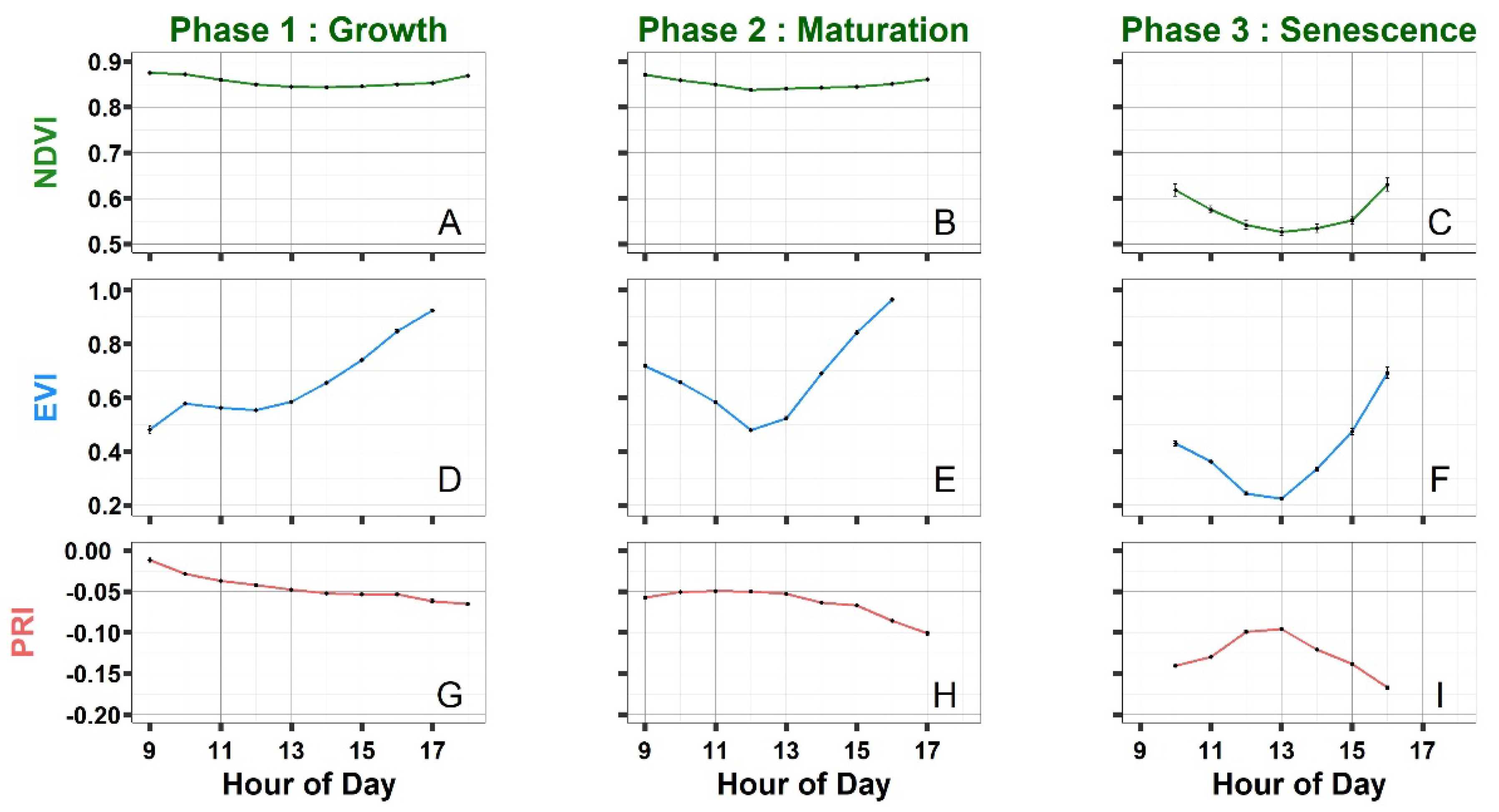
3.2.2. Evolution of Vegetation Indices

The diurnal time course of NDVI, EVI and PRI during the end of vegetation growth of Q. pubescens are shown in Figure 5. No significant changes occur for NDVI; the highest values (about 0.9) were recorded in growth and maturation phases (Figure 5A,B). However, a 1 p.m. depression was shown during the plant’s senescence (Figure 5C). EVI also exhibits a 1 p.m. depression but in both maturation and senescent phases. PRI values are constant during the daytime but the profile in the senescence phase seems to present a peak at 1 p.m. (Figure 5G–I).

3.2.3. Pearson Correlations: SIFs—Environmental Conditions and SIFs—Vegetation Indices

The correlation between CO2 and SIFB (Figure 6G) found at all phases confirms the fact that the mechanisms for regulating photosynthesis light reactions operate mainly at the level of PS II (Photosystem II).
Both SIFs are positively correlated to air temperature and PAR during the growth and acorn maturation season (Figure 6A,C). However, only SIFA is correlated to PAR during senescence (Figure 6A). SIFs are positively correlated to VPD all over the phenology stages (Figure 6E). The correlation between CO2 and SIFB (Figure 6G) found at all phases confirms the fact that the mechanisms for regulating photosynthesis light reactions operate mainly at the level of PS II.

4. Discussion

The aim of this project was to identify effective remote sensing metrics for determining the end of the growing season in a deciduous forest in middle Europe. The main objective was to test the response of the photosynthetic apparatus to climate variations through solar-induced fluorescence (SIF). It also seemed appropriate to find out how SIFs would be influenced by environmental parameters. The period considered was from late summer to autumn, which allowed us to identify three phenological phases of the Downy oak: a growth phase that continues into late summer, followed by a phase of acorn ripening before the actual onset of senescence.
The dynamics of seasonal variation in SIFA and B between early September and early December indicate an end to vegetation on November 20 and 7, respectively (Figure 1). The SIF ratio indicates an alternative date between the two, namely 3 November. As for the apparent value of SIFA, the end of the vegetation period seems to occur earlier, on 31 October. The relationships observed between SIFs and vegetation indices were also analyzed. The sharp drop in PRI from 29 October (Figure 2C, from −0.05 to −0.15) indicates an increase in photoprotection, enabling optimized photosynthetic activity to be maintained despite senescence. This decrease seems to be linked to the break point of SIFA app (31 October). Since SIFA app is correlated with gross primary productivity (GPP), the 31 October date may be considered as the end of the growth period. The 3 days difference of the inflection points between SIFA app (31 October) and NDVI (4 November) are in accordance with the work of Wang [23] who showed that SIF can be used as an early indicator of the end of the carbon dioxide fixation period. In summary, a one-week lag phase is observed (from October 24 to 31), between the onset of senescence and the beginning of the end of the growth period. Furthermore, the breakpoints for SIFB/SIFA and NDVI are very close: 3 November (Figure 1B) and 4 November (Figure 2A), respectively. This suggests that these two variables are highly correlated. Nevertheless, the EVI seems to detect EGS even earlier than SIFA app, with an inflection point on 24 October (Figure 2B), whereas it has been shown that such indices (based on foliage cover and chlorophyll content) are not sensitive enough to capture seasonal vegetation dynamics, at least less so than physiological indices [24,25]. The seasonal dynamics of SIFA and SIFB has been explored in other ecosystems and crops. Because fluorescence emissions at oxygen A line at 760 nm (SIFA) is a component of the FLEX (FLuorescence Explorer) satellite mission, it was relevant to understand its dynamics with field data prior to working with data collected from satellite measurements. SIFA emission was shown to decline by 50% at midday from summer to fall in a subalpine conifer forest in Colorado [26]. In this work, SIF yield variations were associated with photoprotective pigments and photosystem II operating efficiency. In our study, the decline was more accentuated, reaching 80% of the signal. A 2.5-fold decrease in SIFA from May to September was observed in a beech forest [27]. Considering crops as maize, from mature plants to senescence, while little changes occur from SIFB emissions, a significant decrease was exhibited from SIFA emissions [22]. It appears that the phenological decrease in SIFA signal was shown across different ecosystems as well as different photosynthetic traits, namely C3 and C4. The question that arises is related to the mechanistic explanation of SIFA dynamics. Several authors have pointed out that the physiological bases alone could not explain SIFA temporal variations. Indeed, canopy scale, diurnal APAR dynamics and canopy escape probability (ε) are critical for accurately shaping diurnal SIF changes [28,29].
The recorded SIF values are of the same order of magnitude as the data obtained earlier for a deciduous forest during the autumn period [30]. An inversion of SIFs was observed during the phenological stages of Downy oak (Figure 4A–C). The specificities of these three phases may be explained by the ability of chlorophyll to reabsorb its own red fluorescence. Throughout the autumn, the chlorophyll content decreases. During the first phase, the chlorophyll level is still high, and the SIFA emission peak (740 nm) is often higher than SIFB (687 nm) because SIFB emission is strongly impacted by reabsorption. Indeed, chlorophyll A absorption and emission spectra overlaps in the band of 650–700 nm. As the days go by, less and less chlorophyll is present in the leaves; the probability that fluorescence is reabsorbed decreases. SIFB is then less and less impacted by reabsorption and the fluorescence profile gradually returns to that observed in the laboratory, explaining the inversion of intensities between the two SIFs. In field conditions, it has been reported that as the crop begins to senesce, the red/far-red SIF ratio also increases due to a depletion of chlorophylls [31]. The potential scattering effects of branches and leaves on canopy-escaping SIF, canopy structure, as well as changes in photosynthesis activity through photosystems reorganization, should be considered. Also, leaf thickness, and carotenoid contents affect the dynamics of the SIFA/SIFB ratio [32], as well as leaf nitrogen statute [31].
At leaf level, numerous studies have highlighted a sharp reduction in fluorescence emission around midday solar time [33,34] known as “midday depression”. This variation reflects the involvement of plant physiological mechanisms (such as photoprotection processes and stomata aperture regulation) in response to excess light, high temperatures or high VPD values often reached when the sun is at its zenith [34]. SIF “midday depression” has been observed across different ecosystems. An increase of 3% was shown in drought conditions [35]. The diurnal SIF profiles obtained in this study were similar to those for stomatal conductance in oak trees at the OHP site [36], confirming a potential correlation between SIF and GPP. However, for the growth phase of Q. pubescens, the maximum fluorescence was reached at 3 p.m. (Figure 5A), i.e., 2.37 p.m. solar time, and for the last two phenological phases at 2 p.m. (Figure 5B,C), i.e., 1.37 p.m. solar time. The midday depression is therefore shifted a little later, into the afternoon. But this “delayed” midday depression corresponds to the peak of VPD, RH and AT profiles (Supplementary Figure S1). This is in good agreement with a previous work conducted in forest stands, where “the SIF depression” occurred later in the afternoon and was linked to high VPD values [37]. However, this comparison should be treated with caution, as it took place in spring/summer under conditions quite different from our study. Thus, it is likely that water stress might be the determining factor of this shift in SIF depression. Another possible reason for this discrepancy is the impact of the angle of incidence of solar irradiation on the measurement of fluorescence. According to a recent work [38], this angular effect is not negligible. Indeed, the FLOX is set up in such a way that the sun rays arrive perpendicular to the measurement zone at around 2 p.m. This could explain the PAR—SIF offset. Furthermore, this is supported by the fact that the diurnal profile of SIFA app (Figure 4) is itself synchronized with the PAR profile.
Finally, the results of the correlation coefficients highlight two points of interest, in line with the observations detailed above. At the seasonal scale, it appears that SIFA and SIFB are mostly correlated (negatively or positively) with PAR (Figure 3A) and Cloud Index (Figure 3B), and this over all phases. On the other hand, at the diurnal scale, SIFs are less strongly correlated with PAR (Figure 6A) and Cloud Index (Figure 6B), particularly in phases 2 and 3, but more strongly with VPD (Figure 6E), RH (Figure 6D) and AT (Figure 6C). It seems that the environmental factor that has the greatest influence on SIF variations at the daily scale is water stress (through RH, VPD and AT). At the seasonal scale, however, it is light availability. This is in accordance with former studies conducted on maize and wheat [39]. However, most of these environmental parameters covary, which indicates the complexity to disentangle the mechanisms involved.

5. Conclusions

On one hand, it appears that SIF may be used as an earlier proxy for EGS rather than NDVI in the case of a pubescent oak forest, thus demonstrating its potential for accurate modeling of carbon exchanges between Mediterranean forests and the atmosphere. In particular, SIFA apparent is highly linked to PRI and is thus considered as a robust indicator of the end of vegetation period. Seasonal variations in the SIF signal appear to be mainly controlled by light availability, while daily variations are particularly influenced by water stress, through atmospheric Vapor Pressure Deficit, Relative Humidity and Temperature. The positive correlation between apparent SIFA and tropospheric ozone concentrations augurs well for the possible monitoring of forest health using remote sensing, but this will require further investigation. To complete this phenological and functional approach to atmospheric CO2 sequestration, more in-depth studies could focus on the start of the vegetation period, which is often associated with significant variations in chlorophyll biosynthesis and accumulation.

Supplementary Materials

The following supporting information can be downloaded at: https://www.mdpi.com/article/10.3390/rs17071252/s1. Figure S1: Daily averages of environmental conditions at OHP from 30 August to 30 November 2018. A: cloud cover index (Coud Index) and PAR; B: air temperature (AT) and relative humidity (RH); C: vapour pressure deficit (VPD) and soil moisture (SM); D: tropospheric ozone content and CO2; E: wind speed.

Author Contributions

Methodology, J.-P.M., I.X.-R., I.M.R. and T.J.; Validation, T.J.; Investigation, A.B.; Resources, T.J.; Data curation, A.B. and T.J.; Writing—original draft, A.B.; Writing—review & editing, J.-P.M., I.X.-R., I.M.R. and F.M.; Supervision, J.-P.M., I.X.-R. and I.M.R.; Project administration, F.M.; Funding acquisition, F.M. All authors have read and agreed to the published version of the manuscript.

Funding

Funding from AtmoFLEX from ESA, the European Space Agency.

Data Availability Statement

The original contributions presented in this study are included in the article/Supplementary Materials. Further inquiries can be directed to the corresponding author.

Acknowledgments

Funding from AtmoFLEX from ESA, the European Space Agency (Support by the OHP for the mounting of the FLOXBOX, only the one at 100 m), University of Milano c/o Roberto for lending the FLOXBox, COOPERATE database by Armand Rotereau and Gérard Castagnoli, and AtmoSud for ozone data.

Conflicts of Interest

Author Tommaso Julitta was employed by the company JB Hyperspectral Devices GmbH. The remaining authors declare that the research was conducted in the absence of any commercial or financial relationships that could be construed as a potential conflict of interest.

References

  1. Thomson, A.M.; César Izaurralde, R.; Smith, S.J.; Clarke, L.E. Integrated Estimates of Global Terrestrial Carbon Sequestration. Glob. Environ. Change 2008, 18, 192–203. [Google Scholar] [CrossRef]
  2. Archibold, O.W. Temperate Forest Ecosystems. In Ecology of World Vegetation; Springer Science + Business Media: Dordrecht, The Netherlands, 1995; pp. 165–203. ISBN 978-94-010-4008-2. [Google Scholar]
  3. Martin, P.; Nabuurs, G.-J.; Aubinet, M.; Karjalainen, T.; Vine, E.; Kinsman, J.; Heath, L. Carbon Sinks in Temperate Forests1. Annu. Rev. Energy Environ. 2001, 26, 436–465. [Google Scholar] [CrossRef]
  4. Pan, Y.; Birdsey, R.; Fang, J.; Houghton, R.; Kauppi, P.; Kurz, W.; Phillips, O.; Shvidenko, A.; Lewis, S.; Canadell, J.; et al. A Large and Persistent Carbon Sink in the World’s Forests. Science 2011, 333, 988–993. [Google Scholar] [CrossRef] [PubMed]
  5. Xie, J.; Jia, X.; He, G.; Zhou, C.; Yu, H.; Wu, Y.; Bourque, C.P.-A.; Liu, H.; Zha, T. Environmental Control over Seasonal Variation in Carbon Fluxes of an Urban Temperate Forest Ecosystem. Landsc. Urban Plan. 2015, 142, 63–70. [Google Scholar] [CrossRef]
  6. Allaby, M. Temperate Forests (Biomes of the Earth); AbeBooks: Victoria, BC, Canada, 2006; ISBN 9780816053216. [Google Scholar]
  7. Luyssaert, S.; Marie, G.; Valade, A.; Chen, Y.-Y.; Njakou Djomo, S.; Ryder, J.; Otto, J.; Naudts, K.; Lansø, A.; Ghattas, J.; et al. Author Correction: Trade-Offs in Using European Forests to Meet Climate Objectives. Nature 2019, 567, E13. [Google Scholar] [CrossRef]
  8. Vose, J.M.; Peterson, D.L.; Patel-Weynand, T. Effects of Climatic Variability and Change on Forest Ecosystems: A Comprehensive Science Synthesis for the U.S.; General Technical Report PNW-GTR-870; U.S. Department of Agriculture, Forest Service, Pacific Northwest Research Station: Portland, OR, USA, 2012; Volume 870, 265p. [Google Scholar] [CrossRef]
  9. Kim, J.; Woo, H.R.; Nam, H.G. Toward Systems Understanding of Leaf Senescence: An Integrated Multi-Omics Perspective on Leaf Senescence Research. Mol. Plant 2016, 9, 813–825. [Google Scholar] [CrossRef]
  10. Li, W.; Wang, L.; He, Z.; Lu, Z.; Cui, J.; Xu, N.; Jin, B.; Wang, L. Physiological and Transcriptomic Changes During Autumn Coloration and Senescence in Ginkgo Biloba Leaves. Hortic. Plant J. 2020, 6, 396–408. [Google Scholar] [CrossRef]
  11. Wen, C.-H.; Lin, S.-S.; Chu, F.-H. Transcriptome Analysis of a Subtropical Deciduous Tree: Autumn Leaf Senescence Gene Expression Profile of Formosan Gum. Plant Cell Physiol. 2015, 56, 163–174. [Google Scholar] [CrossRef]
  12. Gao, S.; Zhong, R.; Yan, K.; Ma, X.; Chen, X.; Pu, J.; Gao, S.; Qi, J.; Yin, G.; Myneni, R.B. Evaluating the Saturation Effect of Vegetation Indices in Forests Using 3D Radiative Transfer Simulations and Satellite Observations. Remote Sens. Environ. 2023, 295, 113665. [Google Scholar] [CrossRef]
  13. Wang, S.; Zhang, L.; Huang, C.; Qiao, N. An NDVI-Based Vegetation Phenology Is Improved to Be More Consistent with Photosynthesis Dynamics through Applying a Light Use Efficiency Model over Boreal High-Latitude Forests. Remote Sens. 2017, 9, 695. [Google Scholar] [CrossRef]
  14. Frankenberg, C.; Berry, J. 3.10—Solar Induced Chlorophyll Fluorescence: Origins, Relation to Photosynthesis and Retrieval. In Comprehensive Remote Sensing; Liang, S., Ed.; Elsevier: Oxford, UK, 2018; pp. 143–162. ISBN 978-0-12-803221-3. [Google Scholar]
  15. Zhang, J.; Xiao, J.; Tong, X.; Zhang, J.; Meng, P.; Li, J.; Liu, P.; Yu, P. NIRv and SIF Better Estimate Phenology than NDVI and EVI: Effects of Spring and Autumn Phenology on Ecosystem Production of Planted Forests. Agric. For. Meteorol. 2022, 315, 108819. [Google Scholar] [CrossRef]
  16. van der Tol, C.; Julitta, T.; Yang, P.; Sabater, N.; Reiter, I.; Tudoroiu, M.; Schuettemeyer, D.; Drusch, M. Retrieval of Chlorophyll Fluorescence from a Large Distance Using Oxygen Absorption Bands. Remote Sens. Environ. 2023, 284, 113304. [Google Scholar] [CrossRef]
  17. Lelandais, L.; Xueref-Remy, I.; Riandet, A.; Blanc, P.E.; Armengaud, A.; Oppo, S.; Yohia, C.; Ramonet, M.; Delmotte, M. Analysis of 5.5 Years of Atmospheric CO2, CH4, CO Continuous Observations (2014–2020) and Their Correlations, at the Observatoire de Haute Provence, a Station of the ICOS-France National Greenhouse Gases Observation Network. Atmos. Environ. 2022, 277, 119020. [Google Scholar] [CrossRef]
  18. Xueref-Remy, I.; Milne, M.; Zoghbi, N.; Lelandais, L.; Riandet, A.; Armengaud, A.; Gille, G.; Lanzi, L.; Oppo, S.; Brégonzio-Rozier, L.; et al. Analysis of Atmospheric CO2 Variability in the Marseille City Area and the North-West Mediterranean Basin at Different Time Scales. Atmos. Environ. X 2023, 17, 100208. [Google Scholar] [CrossRef]
  19. Alonso, L.; Gomez-Chova, L.; Vila-Frances, J.; Amoros-Lopez, J.; Guanter, L.; Calpe, J.; Moreno, J. Improved Fraunhofer Line Discrimination Method for Vegetation Fluorescence Quantification. IEEE Geosci. Remote Sens. Lett. 2008, 5, 620–624. [Google Scholar] [CrossRef]
  20. Stamford, J.D.; Vialet-Chabrand, S.; Cameron, I.; Lawson, T. Development of an Accurate Low Cost NDVI Imaging System for Assessing Plant Health. Plant Methods 2023, 19, 9. [Google Scholar] [CrossRef]
  21. Muggeo, V. Segmented: An R Package to Fit Regression Models with Broken-Line Relationships. R News 2008, 8, 20–25. [Google Scholar]
  22. Campbell, P.K.E.; Huemmrich, K.F.; Middleton, E.M.; Ward, L.A.; Julitta, T.; Daughtry, C.S.T.; Burkart, A.; Russ, A.L.; Kustas, W.P. Diurnal and Seasonal Variations in Chlorophyll Fluorescence Associated with Photosynthesis at Leaf and Canopy Scales. Remote Sens. 2019, 11, 488. [Google Scholar] [CrossRef]
  23. Wang, F.; Chen, B.; Lin, X.; Zhang, H. Solar-Induced Chlorophyll Fluorescence as an Indicator for Determining the End Date of the Vegetation Growing Season. Ecol. Indic. 2020, 109, 105755. [Google Scholar] [CrossRef]
  24. Dobrowski, S.Z.; Pushnik, J.C.; Zarco-Tejada, P.J.; Ustin, S.L. Simple Reflectance Indices Track Heat and Water Stress-Induced Changes in Steady-State Chlorophyll Fluorescence at the Canopy Scale. Remote Sens. Environ. 2005, 97, 403–414. [Google Scholar] [CrossRef]
  25. Garbulsky, M.F.; Filella, I.; Verger, A.; Peñuelas, J. Photosynthetic Light Use Efficiency from Satellite Sensors: From Global to Mediterranean Vegetation. Environ. Exp. Bot. 2014, 103, 3–11. [Google Scholar] [CrossRef]
  26. Magney, T.S.; Bowling, D.R.; Logan, B.A.; Grossmann, K.; Stutz, J.; Blanken, P.D.; Burns, S.P.; Cheng, R.; Garcia, M.A.; Köhler, P.; et al. Mechanistic Evidence for Tracking the Seasonality of Photosynthesis with Solar-Induced Fluorescence. Proc. Natl. Acad. Sci. USA 2019, 116, 11640–11645. [Google Scholar] [CrossRef] [PubMed]
  27. Kováč, D.; Novotný, J.; Šigut, L.; Ač, A.; Peñuelas, J.; Grace, J.; Urban, O. Estimation of Photosynthetic Dynamics in Forests from Daily Measured Fluorescence and PRI Data with Adjustment for Canopy Shadow Fraction. Sci. Total Environ. 2023, 898, 166386. [Google Scholar] [CrossRef]
  28. Chang, C.Y.; Wen, J.; Han, J.; Kira, O.; LeVonne, J.; Melkonian, J.; Riha, S.J.; Skovira, J.; Ng, S.; Gu, L.; et al. Unpacking the Drivers of Diurnal Dynamics of Sun-Induced Chlorophyll Fluorescence (SIF): Canopy Structure, Plant Physiology, Instrument Configuration and Retrieval Methods. Remote Sens. Environ. 2021, 265, 112672. [Google Scholar] [CrossRef]
  29. Siegmann, B.; Cendrero-Mateo, M.P.; Cogliati, S.; Damm, A.; Gamon, J.; Herrera, D.; Jedmowski, C.; Junker-Frohn, L.V.; Kraska, T.; Muller, O.; et al. Downscaling of Far-Red Solar-Induced Chlorophyll Fluorescence of Different Crops from Canopy to Leaf Level Using a Diurnal Data Set Acquired by the Airborne Imaging Spectrometer HyPlant. Remote Sens. Environ. 2021, 264, 112609. [Google Scholar] [CrossRef]
  30. Yang, X.; Tang, J.; Mustard, J.F.; Lee, J.-E.; Rossini, M.; Joiner, J.; Munger, J.W.; Kornfeld, A.; Richardson, A.D. Solar-Induced Chlorophyll Fluorescence That Correlates with Canopy Photosynthesis on Diurnal and Seasonal Scales in a Temperate Deciduous Forest: Fluorescence and Photosynthesis. Geophys. Res. Lett. 2015, 42, 2977–2987. [Google Scholar] [CrossRef]
  31. Magney, T.S.; Frankenberg, C.; Köhler, P.; North, G.; Davis, T.S.; Dold, C.; Dutta, D.; Fisher, J.B.; Grossmann, K.; Harrington, A.; et al. Disentangling Changes in the Spectral Shape of Chlorophyll Fluorescence: Implications for Remote Sensing of Photosynthesis. J. Geophys. Res. Biogeosciences 2019, 124, 1491–1507. [Google Scholar] [CrossRef]
  32. Wu, L.; Zhang, Y.; Zhang, Z.; Zhang, X.; Wu, Y.; Chen, J.M. Deriving Photosystem-Level Red Chlorophyll Fluorescence Emission by Combining Leaf Chlorophyll Content and Canopy Far-Red Solar-Induced Fluorescence: Possibilities and Challenges. Remote Sens. Environ. 2024, 304, 114043. [Google Scholar] [CrossRef]
  33. Martínez-Ferri, E.; Balaguer, L.; Valladares, F.; Chico, J.M.; Manrique, E. Energy Dissipation in Drought-Avoiding and Drought-Tolerant Tree Species at Midday during the Mediterranean Summer. Tree Physiol. 2000, 20, 131–138. [Google Scholar] [CrossRef]
  34. Pons, T.; Welschen, R. Midday Depression of Net Photosynthesis in the Tropical Rainforest Tree Eperua Grandiflora: Contributions of Stomatal and Internal Conductances, Respiration and Rubisco Functioning. Tree Physiol. 2003, 23, 937–947. [Google Scholar] [CrossRef]
  35. Deng, Z.; Chen, J.; Wang, S.; Li, T.; Huang, K.; Gu, P.; Peng, H.; Chen, Z. Response of Vegetation Photosynthesis to the 2022 Drought in Yangtze River Basin by Diurnal Orbiting Carbon Observatory-2/3 Satellite Observations. J. Remote Sens. 2025, 5, 0445. [Google Scholar] [CrossRef]
  36. Belviso, S.; Reiter, I.M.; Loubet, B.; Gros, V.; Lathière, J.; Montagne, D.; Delmotte, M.; Ramonet, M.; Kalogridis, C.; Lebegue, B.; et al. A Top-down Approach of Surface Carbonyl Sulfide Exchange by a Mediterranean Oak Forest Ecosystem in Southern France. Atmos. Chem. Phys. 2016, 16, 14909–14923. [Google Scholar] [CrossRef]
  37. Paul-Limoges, E.; Damm, A.; Hueni, A.; Liebisch, F.; Eugster, W.; Schaepman, M.E.; Buchmann, N. Effect of Environmental Conditions on Sun-Induced Fluorescence in a Mixed Forest and a Cropland. Remote Sens. Environ. 2018, 219, 310–323. [Google Scholar] [CrossRef]
  38. Biriukova, K.; Celesti, M.; Evdokimov, A.; Pacheco-Labrador, J.; Julitta, T.; Migliavacca, M.; Giardino, C.; Miglietta, F.; Colombo, R.; Panigada, C.; et al. Effects of Varying Solar-View Geometry and Canopy Structure on Solar-Induced Chlorophyll Fluorescence and PRI. Int. J. Appl. Earth Obs. Geoinf. 2020, 89, 102069. [Google Scholar] [CrossRef]
  39. Liu, L.; Zhao, W.; Wu, J.; Liu, S.; Teng, Y.; Yang, J.; Han, X. The Impacts of Growth and Environmental Parameters on Solar-Induced Chlorophyll Fluorescence at Seasonal and Diurnal Scales. Remote Sens. 2019, 11, 2002. [Google Scholar] [CrossRef]
Figure 1. Daily averages of solar-induced fluorescence from 30 August to 30 November 2018. (A): SIFA and SIFB; (B): the ratio of SIFB to SIFA and the apparent SIFA. (A,B) are accompanied by linear regressions with the breakpoint of each variable.
Remotesensing 17 01252 g001
Figure 2. Daily averages of vegetation indices from 30 August to 30 November. (A): Normalized Difference Vegetation Index (NDVI); (B): Enhanced Vegetation Index (EVI); (C): Photochemical Reflectance Index (PRI). The dotted lines indicate the breakpoints and the corresponding dates.
Remotesensing 17 01252 g002
Figure 3. Pearson correlation coefficients of daily SIFs with each environmental parameter and each vegetation index in each phase during autumn 2018. (A): SIFs-PAR; (B): SIFs-Cloud Index; (C): SIFs-Atmosphere Temperature (AT); (D): SIFs-Relative Humidity; (E): SIFs-Vapor Pressure Deficit (VPD); (F): SIFs-Soil Moisture (SM); (G): SIFs-CO2; (H): SIFs-Ozone; (I): SIFs-Wind Speed (WS); (J): SIFs-PRI; (K): SIFs-NDVI; (L): SIFs-EVI.
Remotesensing 17 01252 g003
Figure 4. Hourly mean SIFs on five sunny days for each phase in autumn 2018. (AC): SIFA and SIFB; (DF): SIFA_app; (GI): the ratio of SIFB to SIFA.
Remotesensing 17 01252 g004
Figure 5. Hourly averages of vegetation indices (PRI, NDVI and EVI) over five sunny days for each phase of autumn 2018. (AC): Normalized Difference Vegetation Index (NDVI); (DF): Enhanced Vegetation Index (EVI); (GI): Photochemical Reflectance Index (PRI).
Remotesensing 17 01252 g005
Figure 6. Pearson correlation coefficients of the SIFs with each environmental parameter and each index in integrated time in each phase during autumn 2018. Red: SIFA; Blue: SIFB; Black: SIFA app; Brown: the ratio SIFB/SIFA. (A): SIFs-PAR; (B): SIFs-Cloud Index; (C): SIFs-Atmosphere Temperature (AT); (D): SIFs-Relative Humidity; (E): SIFs-Vapor Pressure Deficit (VPD); (F): SIFs-Soil Moisture (SM); (G): SIFs-CO2; (H): SIFs-Ozone; (I): SIFs-Wind Speed (WS).
Remotesensing 17 01252 g006
Disclaimer/Publisher’s Note: The statements, opinions and data contained in all publications are solely those of the individual author(s) and contributor(s) and not of MDPI and/or the editor(s). MDPI and/or the editor(s) disclaim responsibility for any injury to people or property resulting from any ideas, methods, instructions or products referred to in the content.

