
An Improved Machine Learning-Based Method for Unsupervised Characterisation for Coral Reef Monitoring in Earth Observation Time-Series Data


Abstract
1. Introduction
2. Sentinel-2 Data
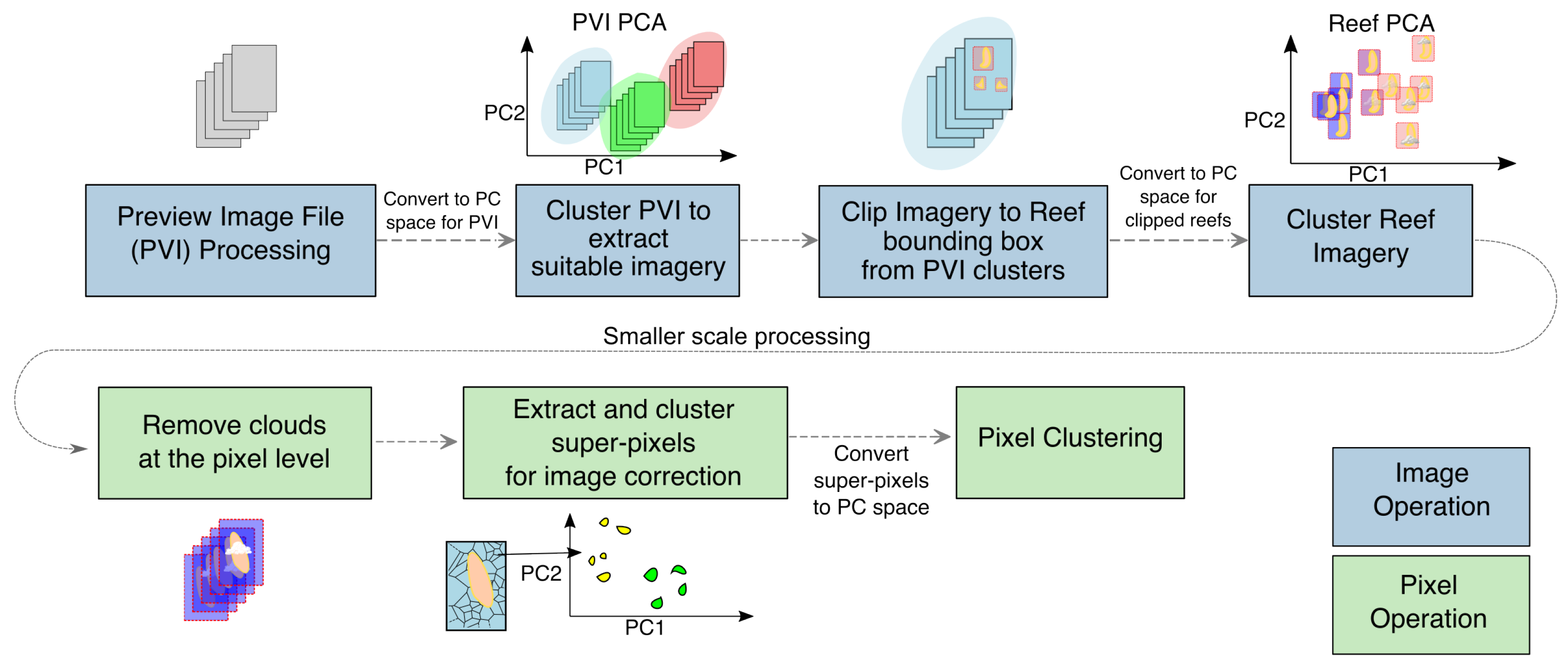
3. Methods
3.1. Libraries
3.2. Background on Machine Learning in Remote Sensing
3.3. Filtering Scenes
- Preparing a training dataset of Sentinel-2 cropped patches of images with a range of imaging conditions from 2015 to 2022 containing 3,150,006 unique pixel values from location 14°56′24.3″S 145°42′00.7″E
- Extracting the image digital number (DN) values of bands 2, 3, 4, and 8 as input values.
- Calculating the mean value of bands 9, 10, 11, and 12 as the target variable.
- Training the XGBoost model to predict the mean target variable based on the input values.
- The algorithm is then tested on a different geographic region within the extracted scenes from 2015 to 2022 (Figure 3), with a total of 70 test images in tile LCD55 from location 14°56′24.3″S 145°42′00.7″E.
- Apply the model to new Sentinel-2 images, predicting the mean value of bands 9, 10, 11, and 12.
- Apply the predetermined threshold to the predicted values (the mean of the target bands).
- Create a binary mask where values above the threshold are classified as cloud/land, and values below are classified as clear water.

3.4. Colour Correction
3.5. Final Classification
4. Results
4.1. Image Selection Using PCA
4.2. Cloud Removal Using XGBoost
4.3. Colour Correction Using Superpixels
4.4. Time-Series Analysis and Change Detection
5. Discussion and Conclusions
Author Contributions
Funding
Data Availability Statement
Conflicts of Interest
Abbreviations
| SWIR | Short-Wave Infrared |
| SLIC | Simple Linear Iterative Clustering |
| PCA | Principal Component Analysis |
| EO | Earth Observation |
Appendix A. Additional Details

Appendix A.1. Image PCA Experiments


Appendix A.2. Cloud Prediction

References
- Goward, S.N.; Williams, D.L.; Arvidson, T.; Rocchio, L.E.; Irons, J.R.; Russell, C.A.; Johnston, S.S. Landsat’s enduring legacy: Pioneering global land observations from space. Photogramm. Eng. Remote Sens. 2022, 88, 357–358. [Google Scholar] [CrossRef]
- eoPortal Directory. IKONOS-2. Available online: https://www.eoportal.org/satellite-missions/ikonos-2#eop-quick-facts-section (accessed on 14 May 2024).
- European Space Agency (ESA). Introducing Sentinel-2. 2024. Available online: https://www.esa.int/Applications/Observing_the_Earth/Copernicus/Sentinel-2 (accessed on 12 March 2025).
- Planet Labs PBC. PlanetScope—Planet Satellites. 2010. Available online: https://support.planet.com/hc/en-us/articles/4407820499217-PlanetScope-Constellation-Sensor-Overview (accessed on 14 May 2024).
- Duarte, C.M. Reviews and Syntheses: Hidden Forests, the Role of Vegetated Coastal Habitats in the Ocean Carbon Budget. Biogeosciences 2017, 14, 301–310. [Google Scholar]
- Tol, R. The Economic Effects of Climate Change. J. Econ. Perspect. 2009, 23, 29–51. [Google Scholar] [CrossRef]
- Goreau, T.F. Mass Expulsion of Zooxanthellae from Jamaican Reef Communities after Hurricane Flora. Science 1964, 145, 383–386. [Google Scholar] [PubMed]
- van Woesik, R.; Kratochwill, C. A Global Coral-Bleaching Database, 1980–2020. Sci. Data 2022, 9, 35058458. [Google Scholar] [CrossRef]
- Belbin, L.; Wallis, E.; Hobern, D.; Zerger, A. The Atlas of Living Australia: History, current state and future directions. Biodivers. Data J. 2021, 9, e65023. [Google Scholar] [CrossRef]
- Rogers, R.; de Oliveira Correal, G.; De Oliveira, T.C.; De Carvalho, L.L.; Mazurek, P.; Barbosa, J.E.F.; Chequer, L.; Domingos, T.F.S.; de Andrade Jandre, K.; Leão, L.S.D.; et al. Coral health rapid assessment in marginal reef sites. Mar. Biol. Res. 2014, 10, 612–624. [Google Scholar] [CrossRef]
- Suan, A.; Franceschini, S.; Madin, J.; Madin, E. Quantifying 3D coral reef structural complexity from 2D drone imagery using artificial intelligence. Ecol. Inform. 2025, 85, 102958. [Google Scholar]
- Casella, E.; Collin, A.; Harris, D.; Ferse, S.; Bejarano, S.; Parravicini, V.; Hench, J.L.; Rovere, A. Mapping coral reefs using consumer-grade drones and structure from motion photogrammetry techniques. Coral Reefs 2017, 36, 269–275. [Google Scholar] [CrossRef]
- McLeod, E.; Shaver, E.C.; Beger, M.; Koss, J.; Grimsditch, G. Using resilience assessments to inform the management and conservation of coral reef ecosystems. J. Environ. Manag. 2021, 277, 111384. [Google Scholar]
- Scopélitis, J.; Andréfouët, S.; Phinn, S.; Arroyo, L.; Dalleau, M.; Cros, A.; Chabanet, P. The next step in shallow coral reef monitoring: Combining remote sensing and in situ approaches. Mar. Pollut. Bull. 2010, 60, 1956–1968. [Google Scholar] [CrossRef] [PubMed]
- Andréfouët, S. Coral reef habitat mapping using remote sensing: A user vs. producer perspective. Implications for research, management and capacity building. J. Spat. Sci. 2008, 53, 113–129. [Google Scholar] [CrossRef]
- Hughes, T.P.; Graham, N.A.; Jackson, J.B.; Mumby, P.J.; Steneck, R.S. Rising to the Challenge of Sustaining Coral Reef Resilience. Trends Ecol. Evol. 2010, 25, 633–642. [Google Scholar] [CrossRef]
- Bruno, J.F.; Selig, E.R.; Casey, K.S.; Page, C.A.; Willis, B.L.; Harvell, C.D.; Sweatman, H.; Melendy, A.M. Thermal Stress and Coral Cover as Drivers of Coral Disease Outbreaks. PLoS Biol. 2007, 5, e124. [Google Scholar] [CrossRef]
- Pandolfi, J.M.; Bradbury, R.H.; Sala, E.; Hughes, T.P.; Bjorndal, K.A.; Cooke, R.G.; McArdle, D.; McClenachan, L.; Newman, M.J.H.; Paredes, G.; et al. Global Trajectories of the Long-Term Decline of Coral Reef Ecosystems. Glob. Trajectories Long-Term Decline Coral Reef Ecosyst. 2003, 301, 955–958. [Google Scholar] [CrossRef]
- Hoegh-Guldberg, O.; Mumby, P.J.; Hooten, A.J.; Steneck, R.S.; Greenfield, P.; Gomez, E.; Harvell, C.D.; Sale, P.F.; Edwards, A.J.; Caldeira, K.; et al. Coral Reefs under Rapid Climate Change and Ocean Acidification. Science 2007, 318, 1737–1742. [Google Scholar] [CrossRef] [PubMed]
- Wicaksono, P.; Fauzan, M.A.; Kumara, I.S.W.; Yogyantoro, R.N.; Lazuardi, W.; Zhafarina, Z. Analysis of reflectance spectra of tropical seagrass species and their value for mapping using multispectral satellite images. Int. J. Remote Sens. 2019, 40, 8955–8978. [Google Scholar] [CrossRef]
- United Nations. Transforming Our World: The 2030 Agenda for Sustainable Development. Resolution A/RES/70/1, United Nations. 2015. Available online: https://sustainabledevelopment.un.org/content/documents/21252030%20Agenda%20for%20Sustainable%20Development%20web.pdf (accessed on 20 March 2025).
- Emsley, D.S. Sen2Coral: Detection of Coral Bleaching from Space. Available online: https://sen2coral.argans.co.uk/ (accessed on 1 May 2024).
- Chan, J.C.W. Shallow water habitats monitoring using simulated PRISMA hyperspectral data and Depth Invariant Index—The case of coral reef in Maldives. IOP Conf. Ser. Earth Environ. Sci. 2022, 1109, 012066. [Google Scholar] [CrossRef]
- Hedley, J.; Roelfsema, C.; Koetz, B.; Phinn, S. Capability of the Sentinel 2 mission for tropical coral reef mapping and coral bleaching detection. Remote Sens. Environ. 2012, 120, 145–155. [Google Scholar] [CrossRef]
- Huang, Y.; Yang, H.; Tang, S.; Liu, Y.; Liu, Y. An Appraisal of Atmospheric Correction and Inversion Algorithms for Mapping High-Resolution Bathymetry Over Coral Reef Waters. IEEE Trans. Geosci. Remote Sens. 2023, 61, 4204511. [Google Scholar] [CrossRef]
- Kutser, T.; Paavel, B.; Kaljurand, K.; Ligi, M.; Randla, M. Mapping shallow waters of the Baltic Sea with Sentinel-2 imagery. In Proceedings of the 2018 IEEE/OES Baltic International Symposium (BALTIC), Klaipeda, Lithuania, 12–15 June 2018; pp. 1–6. [Google Scholar]
- Xu, J.; Zhao, J.; Wang, F.; Chen, Y.; Lee, Z. Detection of coral reef bleaching based on sentinel-2 multi-temporal imagery: Simulation and case study. Front. Mar. Sci. 2021, 8, 584263. [Google Scholar] [CrossRef]
- Main-Knorn, M.; Pflug, B.; Louis, J.; Debaecker, V.; Müller-Wilm, U.; Gascon, F. Sen2Cor for Sentinel-2. In Image and Signal Processing for Remote Sensing XXIII; SPIE: Bellingham, WA, USA, 2017; pp. 37–48. [Google Scholar] [CrossRef]
- Kaufman, Y.J.; Sendra, C. Algorithm for Automatic Atmospheric Corrections to Visible and Near-IR Satellite Imagery. Int. J. Remote Sens. 1988, 9, 1357–1381. [Google Scholar] [CrossRef]
- Whitlock, C.H.; Poole, L.R.; Usry, J.W.; Houghton, W.M.; Witte, W.G.; Morris, W.D.; Gurganus, E.A. Comparison of Reflectance with Backscatter and Absorption Parameters for Turbid Waters. Appl. Opt. 1981, 20, 517–522. [Google Scholar] [CrossRef] [PubMed]
- Lyzenga, D.R. Remote Sensing of Bottom Reflectance and Water Attenuation Parameters in Shallow Water Using Aircraft and Landsat Data. Int. J. Remote Sens. 1981, 2, 71–82. [Google Scholar] [CrossRef]
- Drusch, M.; Del Bello, U.; Carlier, S.; Colin, O.; Fernandez, V.; Gascon, F.; Hoersch, B.; Isola, C.; Laberinti, P.; Martimort, P.; et al. Sentinel-2: ESA’s Optical High-Resolution Mission for GMES Operational Services. Remote Sens. Environ. 2012, 120, 25–36. [Google Scholar]
- Qiu, S.; Zhu, Z.; He, B. Fmask 4.0: Improved cloud and cloud shadow detection in Landsats 4–8 and Sentinel-2 imagery. Remote Sens. Environ. 2019, 231, 111205. [Google Scholar]
- Skakun, S.; Wevers, J.; Brockmann, C.; Doxani, G.; Aleksandrov, M.; Batič, M.; Frantz, D.; Gascon, F.; Gómez-Chova, L.; Hagolle, O.; et al. Cloud Mask Intercomparison eXercise (CMIX): An evaluation of cloud masking algorithms for Landsat 8 and Sentinel-2. Remote Sens. Environ. 2022, 274, 112990. [Google Scholar] [CrossRef]
- Agency, E.S. Sentinel-2 Products Specification Document; Technical Report S2-PDGS-TAS-DI-PSD; European Space Agency: Paris, France, 2021. [Google Scholar]
- Guo, L.J. Balance contrast enhancement technique and its application in image colour composition. Remote Sens. 1991, 12, 2133–2151. [Google Scholar] [CrossRef]
- Liu, J.G.; Mason, P.J. Essential Image Processing and GIS for Remote Sensing; John Wiley & Sons: Hoboken, NJ, USA, 2013. [Google Scholar]
- Lyzenga, D.R. Passive remote sensing techniques for mapping water depth and bottom features. Appl. Opt. 1978, 17, 379–383. [Google Scholar]
- Harahap, S.D.; Wicaksono, P. Relative Water Column Correction Methods for Benthic Habitat Mapping in Optically Shallow Coastal Water. In Recent Research on Geotechnical Engineering, Remote Sensing, Geophysics and Earthquake Seismology; Çiner, A., Ergüler, Z.A., Bezzeghoud, M., Ustuner, M., Eshagh, M., El-Askary, H., Biswas, A., Gasperini, L., Hinzen, K.G., Karakus, M., et al., Eds.; Springer Nature: Cham, Switzerland, 2024; pp. 181–183. [Google Scholar]
- Thalib, M.S.; Nurdin, N.; Aris, A. The Ability of Lyzenga’s Algorithm for Seagrass Mapping using Sentinel-2A Imagery on Small Island, Spermonde Archipelago, Indonesia. IOP Conf. Ser. Earth Environ. Sci. 2018, 165, 012028. [Google Scholar] [CrossRef]
- Pratomo, D.; Cahyadi, M.N.; Hariyanto, I.; Syariz, M.; Putri, S. Lyzenga Algorithm for Shallow Water Mapping Using Multispectral Sentinel-2 Imageries in Gili Noko Waters. BIO Web Conf. 2024, 89, 07006. [Google Scholar] [CrossRef]
- Sutrisno, D.; Sugara, A.; Darmawan, M. The assessment of coral reefs mapping methodology: An integrated method approach. Iop Conf. Ser. Earth Environ. Sci. 2021, 750, 012030. [Google Scholar]
- Manessa, M.D.M.; Kanno, A.; Sagawa, T.; Sekine, M.; Nurdin, N. Simulation-based investigation of the generality of Lyzenga’s multispectral bathymetry formula in Case-1 coral reef water. Estuar. Coast. Shelf Sci. 2018, 200, 81–90. [Google Scholar] [CrossRef]
- Hedley, J.D.; Roelfsema, C.M.; Phinn, S.R.; Mumby, P.J. Environmental and sensor limitations in optical remote sensing of coral reefs: Implications for monitoring and sensor design. Remote Sens. 2012, 4, 271–302. [Google Scholar] [CrossRef]
- European Space Agency. Sentinel-2 Spectral Response Functions (S2-SRF). Document COPE-GSEG-EOPG-TN-15-0007, Issue 3.2. Available online: https://landsat.usgs.gov/landsat/spectral_viewer/bands/Sentinel-2A%20MSI%20Spectral%20Responses.xlsx (accessed on 12 March 2025).
- McKinney, W. Data Structures for Statistical Computing in Python. In Proceedings of the 9th Python in Science Conference, Austin, TX, USA, 28 June–3 July 2010; pp. 56–61. [Google Scholar] [CrossRef]
- The Pandas Development Team. pandas-dev/pandas: Pandas. 2020. Available online: https://zenodo.org/records/13819579 (accessed on 12 March 2025).
- Harris, C.R.; Millman, K.J.; van der Walt, S.J.; Gommers, R.; Virtanen, P.; Cournapeau, D.; Wieser, E.; Taylor, J.; Berg, S.; Smith, N.J.; et al. Array programming with NumPy. Nature 2020, 585, 357–362. [Google Scholar] [CrossRef] [PubMed]
- Pedregosa, F.; Varoquaux, G.; Gramfort, A.; Michel, V.; Thirion, B.; Grisel, O.; Blondel, M.; Prettenhofer, P.; Weiss, R.; Dubourg, V.; et al. Scikit-learn: Machine Learning in Python. J. Mach. Learn. Res. 2011, 12, 2825–2830. [Google Scholar]
- Bradski, G.; Kaehler, A. OpenCV. Dr. Dobb’s J. Softw. Tools 2000, 25. [Google Scholar]
- van der Walt, S.; Schönberger, J.L.; Nunez-Iglesias, J.; Boulogne, F.; Warner, J.D.; Yager, N.; Gouillart, E.; Yu, T.; The Scikit-Image Contributors. Scikit-Image: Image processing in Python. PeerJ 2014, 2, e453. [Google Scholar] [CrossRef]
- Hunter, J.D. Matplotlib: A 2D graphics environment. Comput. Sci. Eng. 2007, 9, 90–95. [Google Scholar] [CrossRef]
- Waskom, M.L. seaborn: Statistical data visualization. J. Open Source Softw. 2021, 6, 3021. [Google Scholar] [CrossRef]
- Chen, T.; Guestrin, C. Xgboost: A scalable tree boosting system. In Proceedings of the 22nd ACM sigkdd International Conference on Knowledge Discovery and Data Mining, San Francisco, CA, USA, 13–17 August 2016; pp. 785–794. [Google Scholar]
- Goswami, A.; Sharma, D.; Mathuku, H.; Gangadharan, S.M.P.; Yadav, C.S.; Sahu, S.K.; Pradhan, M.K.; Singh, J.; Imran, H. Change Detection in Remote Sensing Image Data Comparing Algebraic and Machine Learning Methods. Electronics 2022, 11, 431. [Google Scholar] [CrossRef]
- Bamisile, O.; Cai, D.; Oluwasanmi, A.; Ejiyi, C.; Ukwuoma, C.C.; Ojo, O.; Mukhtar, M.; Huang, Q. Comprehensive assessment, review, and comparison of AI models for solar irradiance prediction based on different time/estimation intervals. Sci. Rep. 2022, 12, 9644. [Google Scholar]
- Zamani Joharestani, M.; Cao, C.; Ni, X.; Bashir, B.; Talebiesfandarani, S. PM2.5 prediction based on random forest, XGBoost, and deep learning using multisource remote sensing data. Atmosphere 2019, 10, 373. [Google Scholar] [CrossRef]
- Boonnam, N.; Udomchaipitak, T.; Puttinaovarat, S.; Chaichana, T.; Boonjing, V.; Muangprathub, J. Coral Reef Bleaching under Climate Change: Prediction Modeling and Machine Learning. Sustainability 2022, 14, 6161. [Google Scholar] [CrossRef]
- White, E.; Amani, M.; Mohseni, F. Coral Reef Mapping Using Remote Sensing Techniques and a Supervised Classification Algorithm. Adv. Environ. Eng. Res. 2021, 2, 28. [Google Scholar]
- Pavoni, G.; Corsini, M.; Ponchio, F.; Muntoni, A.; Edwards, C.; Pedersen, N.; Sandin, S.; Cignoni, P. TagLab: AI-assisted Annotation for the Fast and Accurate Semantic Segmentation of Coral Reef Orthoimages. J. Field Robot. 2022, 39, 246–262. [Google Scholar]
- Zeng, R.; Hochberg, E.J.; Candela, A.; Wettergreen, D.S. Spectral Unmixing and Mapping of Coral Reef Benthic Cover with Deep Learning. In Proceedings of the 2022 12th Workshop on Hyperspectral Imaging and Signal Processing: Evolution in Remote Sensing (WHISPERS), Rome, Italy, 13–16 September 2022; pp. 1–5. [Google Scholar]
- Li, J.; Knapp, D.E.; Fabina, N.S.; Kennedy, E.V.; Larsen, K.; Lyons, M.B.; Murray, N.J.; Phinn, S.R.; Roelfsema, C.M.; Asner, G.P. A Global Coral Reef Probability Map Generated Using Convolutional Neural Networks. Coral Reefs 2020, 39, 1805–1815. [Google Scholar] [CrossRef]
- Sheng, V.S.; Provost, F.; Ipeirotis, P.G. Get Another Label? Improving Data Quality and Data Mining Using Multiple, Noisy Labelers. In Proceedings of the 14th ACM SIGKDD International Conference on Knowledge Discovery and Data Mining, Las Vegas, NV, USA, 24–27 August 2008; pp. 614–622. [Google Scholar]
- Bishop, C. Pattern Recognition and Machine Learning; Springer: New Delhi, India, 2006; Volume 2, pp. 5–43. [Google Scholar]
- Ester, M.; Kriegel, H.P.; Sander, J.; Xu, X. A density-based algorithm for discovering clusters in large spatial databases with noise. In KDD; ACM: New York, NY, USA, 1996; Volume 96, pp. 226–231. [Google Scholar]
- UNEP-WCMC; WorldFish Centre; WRI; TNC. Global Distribution of Coral Reefs, Compiled from Multiple Sources Including the Millennium Coral Reef Mapping Project; Version 4.1, updated by UNEP-WCMC. Includes contributions from IMaRS-USF and IRD (2005), IMaRS-USF (2005) and Spalding et al. (2001); UN Environment Programme World Conservation Monitoring Centre: Cambridge, UK, 2021. [Google Scholar] [CrossRef]
- Sentinel Hub. Sentinel Hub’s Cloud Detector for Sentinel-2 Imagery. 2024. Available online: https://github.com/sentinel-hub/sentinel2-cloud-detector (accessed on 12 March 2025).
- Abdul Gafoor, F.; Al-Shehhi, M.R.; Cho, C.S.; Ghedira, H. Gradient Boosting and Linear Regression for Estimating Coastal Bathymetry Based on Sentinel-2 Images. Remote Sens. 2022, 14, 5037. [Google Scholar] [CrossRef]
- Krishnaraj, A.; Honnasiddaiah, R. Remote sensing and machine learning based framework for the assessment of spatio-temporal water quality in the Middle Ganga Basin. Environ. Sci. Pollut. Res. 2022, 29, 64939–64958. [Google Scholar]
- Friedman, J.H. Greedy function approximation: A gradient boosting machine. Ann. Stat. 2001, 29, 1189–1232. [Google Scholar] [CrossRef]
- Jin, Q.; Fan, X.; Liu, J.; Xue, Z.; Jian, H. Estimating tropical cyclone intensity in the South China Sea using the XGBoost Model and FengYun Satellite images. Atmosphere 2020, 11, 423. [Google Scholar] [CrossRef]
- Bhagwat, R.U.; Shankar, B.U. A novel multilabel classification of remote sensing images using XGBoost. In Proceedings of the 2019 IEEE 5th International Conference for Convergence in Technology (I2CT), Bombay, India, 29–31 March 2019; pp. 1–5. [Google Scholar]
- Shao, Z.; Ahmad, M.N.; Javed, A. Comparison of Random Forest and XGBoost Classifiers Using Integrated Optical and SAR Features for Mapping Urban Impervious Surface. Remote Sens. 2024, 16, 665. [Google Scholar] [CrossRef]
- Niazkar, M.; Menapace, A.; Brentan, B.; Piraei, R.; Jimenez, D.; Dhawan, P.; Righetti, M. Applications of XGBoost in water resources engineering: A systematic literature review (December 2018–May 2023). Environ. Model. Softw. 2024, 174, 105971. [Google Scholar]
- S2 Processing—Sentiwiki.copernicus.eu. Available online: https://sentiwiki.copernicus.eu/web/s2-processing (accessed on 1 February 2025).
- Zhu, Z.; Wang, S.; Woodcock, C.E. Improvement and expansion of the Fmask algorithm: Cloud, cloud shadow, and snow detection for Landsats 4–7, 8, and Sentinel 2 images. Remote Sens. Environ. 2015, 159, 269–277. [Google Scholar]
- Wieland, M.; Fichtner, F.; Martinis, S. UKIS-CSMASK: A Python Package for Multi-Sensor Cloud and Cloud Shadow Segmentation. Int. Arch. Photogramm. Remote Sens. Spat. Inf. Sci. 2022, XLIII-B3-2022, 217–222. [Google Scholar] [CrossRef]
- Green, E.; Edwards, A.; Clark, C. Remote Sensing Handbook for Tropical Coastal Management; UNESCO Publishing: Paris, France, 2000. [Google Scholar]
- Achanta, R.; Shaji, A.; Smith, K.; Lucchi, A.; Fua, P.; Süsstrunk, S. SLIC Superpixels Compared to State-of-the-Art Superpixel Methods. IEEE Trans. Pattern Anal. Mach. Intell. 2012, 34, 2274–2282. [Google Scholar] [CrossRef] [PubMed]
- Zhao, X.; Qi, C.; Zhu, J.; Su, D.; Yang, F.; Zhu, J. A satellite-derived bathymetry method combining depth invariant index and adaptive logarithmic ratio: A case study in the Xisha Islands without in-situ measurements. Int. J. Appl. Earth Obs. Geoinf. 2024, 134, 104232. [Google Scholar]
- Siregar, V.; Agus, S.; Subarno, T.; Prabowo, N. Mapping shallow waters habitats using OBIA by applying several approaches of depth invariant index in North Kepulauan Seribu. IOP Conf. Ser. Earth Environ. Sci. 2018, 149, 012052. [Google Scholar]
- Manuputty, A.; Lumban-Gaol, J.; Agus, S.B. Seagrass mapping based on satellite image Worldview-2 by using depth invariant index method. ILMU Kelaut. Indones. J. Mar. Sci. 2016, 21, 37–44. [Google Scholar]
- Aljahdali, M.H.; Elhag, M. Calibration of the depth invariant algorithm to monitor the tidal action of Rabigh City at the Red Sea Coast, Saudi Arabia. Open Geosci. 2020, 12, 1666–1678. [Google Scholar]
- Komatsu, T.; Hashim, M.; Nurdin, N.; Noiraksar, T.; Prathep, A.; Stankovic, M.; Son, T.P.H.; Thu, P.M.; Van Luong, C.; Wouthyzen, S.; et al. Practical mapping methods of seagrass beds by satellite remote sensing and ground truthing. Coast. Mar. Sci. 2020, 43, 1–25. [Google Scholar]
- Otsu, N. A threshold selection method from gray-level histograms. Automatica 1975, 11, 23–27. [Google Scholar]
- Liao, P.S.; Chen, T.S.; Chung, P.C. A Fast Algorithm for Multilevel Thresholding. J. Inf. Sci. Eng. 2001, 17, 713–727. [Google Scholar]
- Rousseeuw, P.J. Silhouettes: A graphical aid to the interpretation and validation of cluster analysis. J. Comput. Appl. Math. 1987, 20, 53–65. [Google Scholar] [CrossRef]
- European Space Agency. Sentinel-2 Operations. 2024. Available online: https://www.esa.int/Enabling_Support/Operations/Sentinel-2_operations (accessed on 12 March 2024).


| Band | (nm)/ (nm) | Purpose | Resolution |
|---|---|---|---|
| B1 | 443/20 | Atmos. corr. (aerosol) | 60 m |
| B2 | 490/65 | Veg. senescence, Atmos. corr. | 10 m |
| B3 | 560/35 | Total chlorophyll | 10 m |
| B4 | 665/30 | Max chlorophyll absorption | 10 m |
| B5, B6 | 705, 740/15 | Red edge, Atmos. corr. | 20 m |
| B7 | 783/20 | LAI, NIR edge | 20 m |
| B8 | 842/105 | LAI | 10 m |
| B8a | 865/20 | NIR plateau, chlorophyll, biomass, LAI | 20 m |
| B9 | 945/20 | Water vapour, Atmos. corr. | 60 m |
| B10 | 1375/30 | Cirrus detection | 60 m |
| B11 | 1610/90 | Lignin, biomass, snow/ice/cloud | 20 m |
| B12 | 2190/180 | Veg. conditions, soil erosion, burn scars | 20 m |
| Band | (nm) | Description | Role |
|---|---|---|---|
| 2 | 490 | Blue | Input Band |
| 3 | 560 | Green | Input Band |
| 4 | 665 | Red | Input Band |
| 8 | 842 | Near-Infrared | Input Band |
| 9 | 945 | Water Vapor | Target Band |
| 10 | 1375 | Cirrus | Target Band |
| 11 | 1610 | Short-Wave Infrared 1 | Target Band |
| 12 | 2190 | Short-Wave Infrared 2 | Target Band |
Disclaimer/Publisher’s Note: The statements, opinions and data contained in all publications are solely those of the individual author(s) and contributor(s) and not of MDPI and/or the editor(s). MDPI and/or the editor(s) disclaim responsibility for any injury to people or property resulting from any ideas, methods, instructions or products referred to in the content. |
© 2025 by the authors. Licensee MDPI, Basel, Switzerland. This article is an open access article distributed under the terms and conditions of the Creative Commons Attribution (CC BY) license (https://creativecommons.org/licenses/by/4.0/).
Share and Cite
AlZayer, Z.; Mason, P.; Platt, R.; John, C.M. An Improved Machine Learning-Based Method for Unsupervised Characterisation for Coral Reef Monitoring in Earth Observation Time-Series Data. Remote Sens. 2025, 17, 1244. https://doi.org/10.3390/rs17071244
AlZayer Z, Mason P, Platt R, John CM. An Improved Machine Learning-Based Method for Unsupervised Characterisation for Coral Reef Monitoring in Earth Observation Time-Series Data. Remote Sensing. 2025; 17(7):1244. https://doi.org/10.3390/rs17071244
Chicago/Turabian StyleAlZayer, Zayad, Philippa Mason, Robert Platt, and Cédric M. John. 2025. "An Improved Machine Learning-Based Method for Unsupervised Characterisation for Coral Reef Monitoring in Earth Observation Time-Series Data" Remote Sensing 17, no. 7: 1244. https://doi.org/10.3390/rs17071244
APA StyleAlZayer, Z., Mason, P., Platt, R., & John, C. M. (2025). An Improved Machine Learning-Based Method for Unsupervised Characterisation for Coral Reef Monitoring in Earth Observation Time-Series Data. Remote Sensing, 17(7), 1244. https://doi.org/10.3390/rs17071244