Validating HF Radar Current Accuracy via Lagrangian Measurements and Radar-to-Radar Comparisons in Highly Variable Surface Currents

Abstract

The validation of HF radar systems remains an area with significant scope for advancement, particularly in terms of linking data quality with system operational parameters, fully utilizing the potential of redundant data (e.g., overlapping radial measurements), and accurately capturing the spatiotemporal variability observed by independent devices, such as drifters. In this study, we conducted a large-scale Lagrangian measurement campaign in the Tuscan Archipelago, aimed at validating surface current data from the HF radar network. This radar network, a recent addition to the area, monitors an oceanographic region critical to Mediterranean dynamics. The validation was executed using different approaches: a Eulerian method, comparing the radial velocities measured by radar with drifter-derived velocities along radial directions; a Lagrangian method, contrasting the observed drifter trajectories with the synthetic virtual trajectories generated from radar-based flow fields; and radar-to-radar comparisons with the concurrent utilization of two radars in same point. Through fine-tuning of the quality control parameters and an analysis of the impact of different thresholds of such parameters, we assessed the radar’s ability to capture dynamic processes, identifying both strengths and limitations. Our results not only confirm the utility of HF radar in coastal monitoring but also provide a basis for improving calibration strategies, ultimately supporting more accurate, high-resolution radar observations in complex marine environments.

1. Introduction

In recent years, the use of HF radar to improve our knowledge of marine circulation and coastal processes has become increasingly important for environmental, economic, and safety reasons. Continuous, real-time monitoring of surface currents supports a wide range of applications, including emergency management services such as search and rescue (SAR) operations, oil spill forecasting, the identification of accumulation areas for micro and macroplastics, and the study of larval transport and connectivity.

HF radar-based marine monitoring systems are expanding worldwide, including in the Mediterranean, one of the most densely exploited marine areas globally. A comprehensive review of HF radar technology and its potential, with a particular focus on the Mediterranean, is available in [1,2]. In the Northwestern Mediterranean, particularly the Northern Tyrrhenian and Ligurian–Provençal basins, the development of HF radar-based monitoring systems has been notable. Several initiatives have significantly increased the availability of radar data, such as the LaMMA Consortium’s efforts in collaboration with CNR, the University of Toulon, and through projects like IMPACT, SICOMAR, and SICOMAR+ (EU Interreg IT-FR), to monitor the marine area of the North Tyrrhenian and Ligurian Seas, which includes the Cetacean Sanctuary and the Tuscany Archipelago.

However, like many similar systems worldwide [3,4,5], HF radar systems require continuous maintenance. Malfunctions, environmental, and anthropogenic interferences can degrade the radar signal, affecting data accuracy. Periodic validation of radar data is necessary, typically using independent observations from tools such as ADCP current meters or drifters [6,7,8,9,10].

Drifters (or drifting buoys) are extensively used to validate HF radar observations. They provide high-resolution measurements of surface currents at small time intervals (e.g., every 5 min) and spatial scales (a few meters), while HF radar typically averages data over longer periods (hourly) and larger spatial cells (several kilometers). This spatial and temporal difference means that HF radar data cannot resolve fine-scale processes like small eddies or localized shear. Despite this, various studies have confirmed the validity of drifters in assessing HF radar data reliability [11,12,13,14,15,16]. These studies, conducted in offshore and shallow waters, compared drifter velocities to those derived from HF radar (Eulerian approach) or compared real drifter trajectories to virtual drifters driven by HF radar data (Lagrangian approach).

Drifters such as CODE buoys are ideal for tracking upper-ocean currents within the mixed layer [17], providing valuable information for validating HF radar measurements, which primarily sample surface currents. However, it is important to recognize that HF radar can sample currents deeper than a few centimeters and extend to several meters, influenced by Bragg resonant interactions with ocean surface waves [18]. As a result, HF radar data may not capture hydrodynamic subtleties, such as shear, shallow water effects, and Stokes drift, which drifters can track more effectively.

This study focuses on validating HF radar observations in the complex and ecologically significant area of the Tuscan Archipelago (Figure 1), characterized by a rugged coastline, islands, straits, and highly variable meteorological conditions that generate marine circulation with marked seasonal and sub-seasonal variability [19,20,21,22,23]. The aim of this work is to validate a new HF radar system in an area previously not covered by similar monitoring systems, where important oceanographic processes, such as the water mass exchanges between the Tyrrhenian and Ligurian seas, are still not fully understood. Additionally, this area is of significant biodiversity value, as it is part of the Pelagos Sanctuary, the largest European marine area under special protection.

To validate the HF radar data, we employ both Eulerian and Lagrangian approaches using a large number of drifters deployed during an oceanographic campaign to study circulation between the Northern Tyrrhenian and Ligurian seas. This study examines the performance of the HF radar system using traditional statistical methods (e.g., correlation and error analysis), while also exploring methods like Kriging for improving velocity estimates. Kriging is used to interpolate drifter data, addressing spatial correlations in the measurements and local flow fluctuations.

The validation of radar data with drifters serves as both a diagnostic tool for system performance and a means of improving the quality of radar measurements. The integration of different radar measurements from multiple antennas, including radar-to-radar comparisons for closely placed systems like those on Tino Island (operating at 25 MHz and 13.5 MHz), provides further insights into the data quality.

This study also discusses the limitations of HF radar in measuring small eddies and highly variable currents with the same accuracy as drifters, emphasizing the importance of quality control in improving data reliability. Fine-tuning quality control parameters, in line with European standards [24], ensures that the data produced by the system meets a high standard of accuracy, even if this results in a reduction in the total volume of data.

2. Materials and Methods

2.1. The HF Radar Network Covering the Tuscany Coast

The HF radar network, installed by the LaMMA Consortium and the Tuscany Region, covers a large marine area between the Northern Tyrrhenian Sea and the Ligurian Sea (Figure 1a and Figure 2) and is part of a large cross-border network connecting the Northwest Mediterranean arc that was implemented in collaboration with CNR ISMAR and the University of Toulon. This network is currently expanding due to some recent initiatives such as the INTERREG Italy–France program projects and PNRRs (National Recovery and Resilience Plans). In this work, only the data produced by the radar network on the Ligurian Sea has been taken into consideration. The LaMMA HF radar network includes two SeaSonde stations installed on the Tuscan coast at Livorno (LIVO) and San Vincenzo (SVIN), operational since 2015, and a SeaSonde station located on the Isola del Tino (TINO), operational since 2018. The HF radar system covers an extended area of the Tuscan Archipelago from Elba Island up to the Gulf of Spezia. The CODAR antennas operate at a frequency of 13.5 MHz and a bandwidth of 100 kHz. The radial resolution is about 1.5 km, reporting current measurements at 5° spacing at about 0.9 m from the surface at an hourly frequency. The total velocity resolution is 3 km, and the transmission power is about 40 W. Under optimal conditions, each radar can reach a coverage of about 80–100 km. Measurements are automatically synchronized with the central calculation server, belonging to the European HFR Node, which combines the radial velocity fields into total velocity fields, applies the quality control (QC) procedures on both the radial and total data, and stores them in a netCDF format. The CNR-ISMAR SeaSonde HF radar is located on the Isola del Tino (TINO25) and operates at a frequency of 25 MHz with a maximum range of approximately 35–45 km; the radial and angular resolutions are 1 km and 5°, respectively. It was installed on the Isola del Tino in the summer of 2016, located a few tens of meters from the LaMMA radar [25]. The processing, data transfer, and quality check procedures are the same as for other radars. This dataset is freely downloadable from the thread’s servers [26].

2.2. Quality Assurance (QA) and Quality Control (QC) Parameters for the HF Radars

The verification of the HF radar data occurs in two phases: an initial check during signal acquisition (QA—quality assurance) and a subsequent check on the processed data (QC—quality control). QA focuses on the optimal radar setup, including hardware and software configurations, vendor tests, and calibration. QC ensures the validity and accuracy of the measurements. Both QA and QC rely on specific parameters with adaptable thresholds, which vary based on installation characteristics and are still being refined by the scientific community.

The SeaSonde QA suite generates diagnostic files containing hardware data to monitor the transmitter, receiver, and antennas. These files also store key radial parameters, such as range, radial count per cell, and bearing values. Analyzing these diagnostics helps detect anomalies that might not be evident from radar output maps alone. Therefore, these parameters are often called “performance metrics”.

Overall, about seventy hardware and software parameters can be monitored. Some are interdependent, e.g., high transmitter reflected power (XARW) may indicate a hardware issue, leading to low forward power (XAFW), reduced signal-to-noise ratio (SNR), and fewer detected radial vectors. Others are independent, e.g., high transmitter or receiver temperatures may not immediately affect measurements but can damage electronic components over time.

During post-processing, all radial vectors undergo QC following European standards, which include checks like velocity and variance thresholds, median filtering, and radial count. Some standard QC parameters, such as AVRB_QC (average radial bearing) and TIME_QC (temporal derivative), do not apply to our beamforming-based radars. A summary of the parameters used in this study for QC is provided in the lists in

Table 1. Summary table of the European data QC standards (CMEMS, 2017) used in this study.

QC Parameters	Description
VART_QC (Variance Threshold Quality Flags)	This test labels radial vectors, whose temporal variance is larger than a maximum threshold, with a “bad data” flag, otherwise with a “good data” flag. Default threshold value is 1 m/s.
MDFL_QC (Median Filter)	For each source vector, the median of all velocities within a radius of <RCLim> and whose vector bearing (angle of arrival at site) is also within an angular distance of <AngLim> degrees from the source vector’s bearing is evaluated. If the difference between the vector’s velocity and the median velocity is greater than a threshold, then the vector is labeled with a “bad_data” flag. Otherwise, it is labeled with a “good_data” flag. Default threshold value is 1 m/s (with AngLim = 30° and RCLim = 5)
RDCT_QC (Radial Count Quality Flag)	Test labeling the entire data file having a number of radial velocity vectors larger than the threshold with a “good data” flag, otherwise with “bad data”. Default value is 200.
(CSPD_QC Maximum Velocity Threshold)	This test labels radial velocity vectors whose module is larger than a maximum velocity threshold with a “bad data” flag, otherwise with a “good data” flag. Default value is 1.2 m/s.

. For a more detailed discussion of QA/QC for HF radar surface data, refer to the literature [27,28,29]. This study examines the impact of suboptimal QA parameters on the proper functioning of the radar and the benefits of QC parameter calibration when comparing with drifter current data.

2.3. The Drifter Dataset

In October 2020, in the Southern Ligurian Sea (SLS), a field measurement campaign was organized by the CMRE [30]. A huge number of low-cost freely drifting Lagrangian instruments, equipped with oceanographic and acoustic sensors, were deployed in a restricted area, covered by the HF radars, and tracked over time.

The deployed drifters included CODE, SVP, DWS, DARPA PARC, and River-type models. Among them, CODE drifters measure currents within the first meter of the water column and are minimally affected by wind. Under strong wind conditions, slippage due to wind and waves is negligible (around 0.1% of wind intensity), while wind-driven currents flow downwind at approximately 1% of the wind speed [31,32].

For this experiment, LaMMA used MAXO-manufactured CODE drifters equipped with a SPOT Globalstar TRACE module, featuring a high-accuracy GPS receiver (<10 m) and a 5 min transmission frequency. Their velocity accuracy is about 3 cm/s.

For HF radar validation purposes, 26 drifters were released within a few hours to form a square array of 3 km × 3 km in a small area off the SLS (centered on Lat: 43°16′N, Lon: 10°14′E) about 100 m deep. All drifters were released within a few hours. Some of them recovered after 1–3 days (5 on 26), and others beached after a few days. To transmit their position ashore in near real time, drifters closer to the coast used cellular transmission, whereas those farther offshore automatically switched to the satellite connection. Approximately in one month, most of the drifters were beached or outside the coverage area of the HF radar network (Figure 1a,c).

We analyzed the period between 8 October and 8 November 2020. Due to episodic malfunctions, drifter trajectories present some gaps, and the subsequent comparison with real drifters was performed in sub-intervals. The speed of each drifter was calculated as the ratio between the distance traveled and the travel time at 5 min steps.

In addition, we considered the data collected by a few drifters released by IFREMER in the SLS close to Bastia (Corse, Figure 1c) from May to September 2019 (dataset is available from the Pacific Gyre web platform [33]). In this case, CARTHE (Consortium for Advanced Research on Transport of Hydrocarbon in the Environment) drifters were used with a data transmission frequency of 5 min. This type of drifter accurately follows the currents in the upper 0.60 m. It presents minimal wave rectification issues and is poorly affected by wind [34]. Pairs of CODE and CARTHE drifters deployed together in the open ocean showed similar behavior, and despite their different designs, they measure surface currents in approximately the same way [35].

2.4. Comparison of Radial Velocities (Eulerian Approach)

The comparison between the radial velocity measured by each HF radar antenna with the Eulerian velocity extracted from the drifter’s trajectory and projected onto the radial direction can be summarized as follows:

(i)

First, the zonal and meridional velocity components are determined from the trajectory of each drifter. The calculation is made on the Cartesian space by means of first-order finite differences, assigning the velocity to the midpoint between two consecutive coordinates. The m_map [36] tool was used to pass from the geographical to the Cartesian space. The values of velocities and positions are then hourly averaged;

(ii)

For every drifter position and every time step, the four surrounding radial velocity values were used to linearly interpolate the radial velocities at the drifter position, then the obtained value was hourly averaged to get Ur (the radial velocity component estimated by radars);

(iii)

Drifter velocity was projected onto the radial direction to get Ud (herein, the radial velocity component measured by drifters) and compared it to Ur;

(iv)

To refine the velocity estimates, particularly in areas with high spatial variability, the Kriging method was applied to the drifter trajectories.

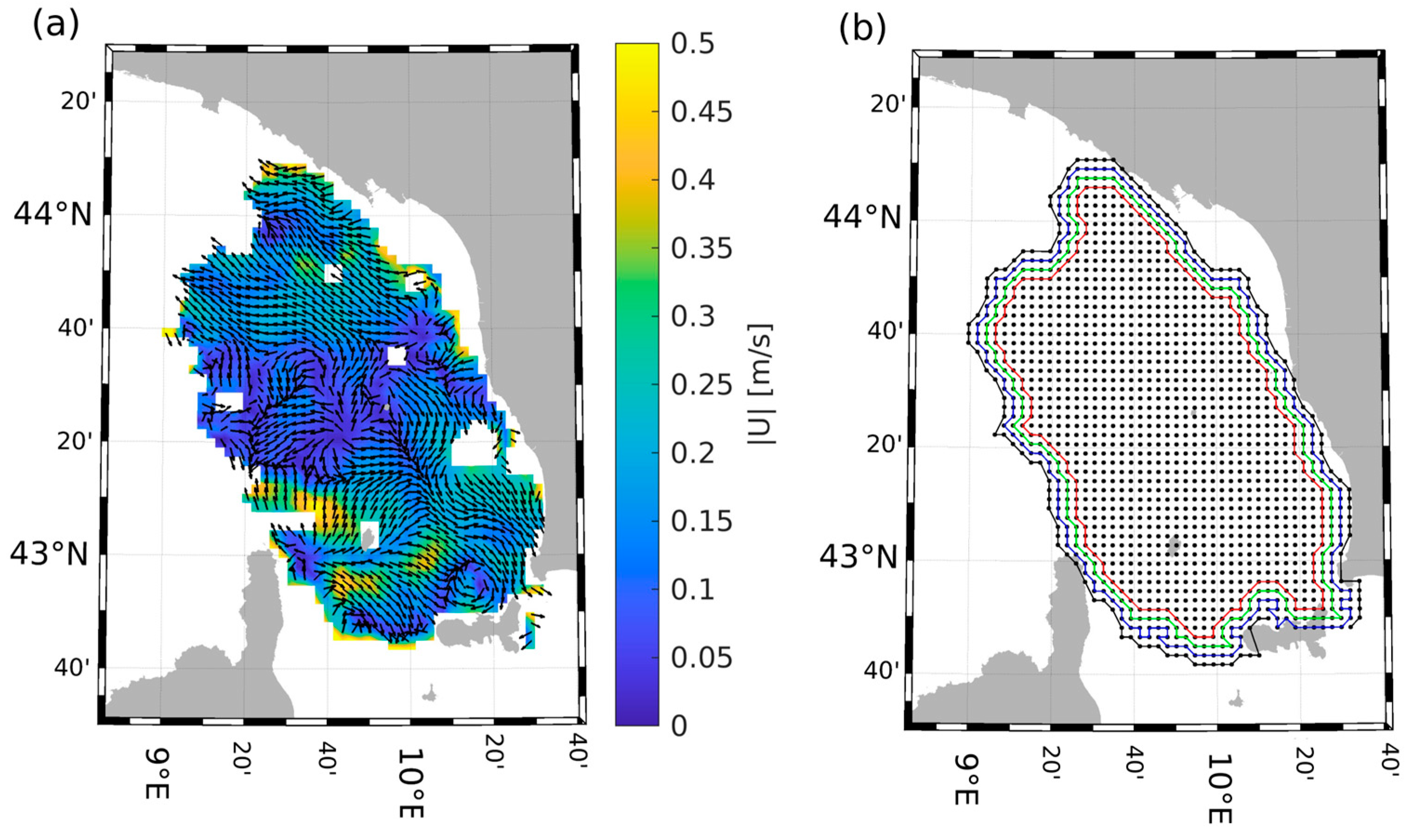
2.5. Application of Kriging for Velocity Estimation

In this study, the Kriging method [37,38] was applied to enhance the estimation of surface current velocities at drifter sampling points. Since drifters provide only position data, their velocities must be derived, making interpolation a crucial step. An analysis of drifter trajectories revealed significant flow variability, requiring a method capable of capturing both local fluctuations and overall trends. Kriging, which estimates values at unsampled locations based on spatial correlations, was implemented to refine these velocity estimations. The method assumes that drifter-derived velocities exhibit spatial correlation, which decreases with distance. This relationship is modeled using an exponential covariance function, defined by these key parameters: the ‘range’ (the distance beyond which correlation becomes negligible), the ‘nugget’ (accounting for small errors or noise in the data), and the ‘sill’ (total variance).

To optimize computational efficiency, interpolation is performed within a local grid centered on each drifter position. The process begins with the computation of the covariance matrix and autocorrelation functions to capture the spatial relationships among sampled points. The model then estimates the velocities both at the unsampled locations and at the drifter sampling points, where it provides more reliable velocity values by better following the drifter’s trajectory. Additionally, Kriging effectively approximates velocities in sections where gaps or interruptions occur, improving the overall representation of the current field.

To achieve this, a buffer zone with a spatial radius of 1000 units is defined around each drifter position, within which the covariance matrix is computed for all pairs of points within this area. The spatial distance between each pair (i,j) is calculated using the Euclidean norm, forming a symmetric distance matrix dij. The covariance matrix is then built using an exponential variogram model:

$$\mathrm{C}\left(\mathrm{dij}\right)=sill·e^{-dij/range}+\mathrm{nugget}·\mathrm{\delta }\left(\mathrm{dij}\right),$$

(1)

where C(dij) represents the covariance between points i, e, and j, and the parameters sill, range, and the nugget defines the spatial correlation structure, which in our case is set to 1, 100, and 0.1, respectively. The choice of these variogram parameters was based on a balance between capturing the spatial variability of the surface current velocities and minimizing the model complexity. The nugget value of 0.1, in particular, represents a small but non-negligible level of local variability or measurement error, which is realistic given the observed standard deviation of the drifter velocities (~0.15).

δ(dij) is the Kronecker delta, which is 1 when d = 0 and 0 otherwise.

To determine the optimal weights for Kriging interpolation, we solve the following linear system:

$$\left(\begin{array}{cc}C& 1\\ 1^T& 0\end{array}\right)\left(\begin{array}{c}w\\ \lambda \end{array}\right)=\left(\begin{array}{c}c\\ 1\end{array}\right),$$

(2)

where w is the vector of Kriging weights, and λ is a Lagrange multiplier ensuring unbiased estimation. The vector c contains the covariances between the observation points and the location where interpolation is performed. The estimated velocity components are then obtained as:

$$\widehat{\mathit{u}}=w^{T}u\widehat{\mathit{v}}=w^{T}v,$$

(3)

where u and v are the measured velocity components derived from position differences at the surrounding drifter locations. This approach ensures that velocity estimates incorporate spatial correlation while minimizing estimation variance.

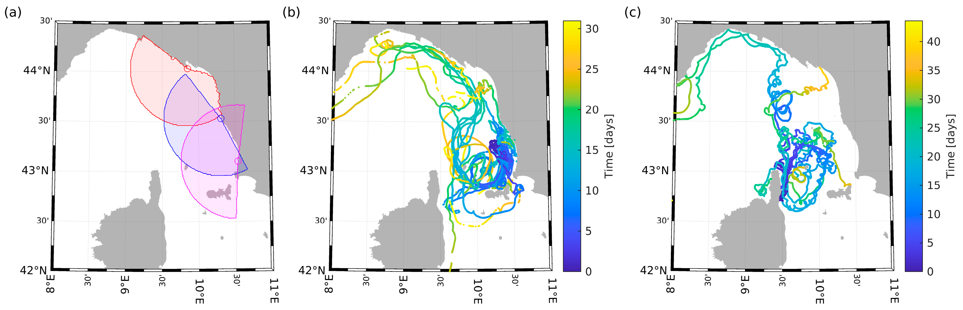
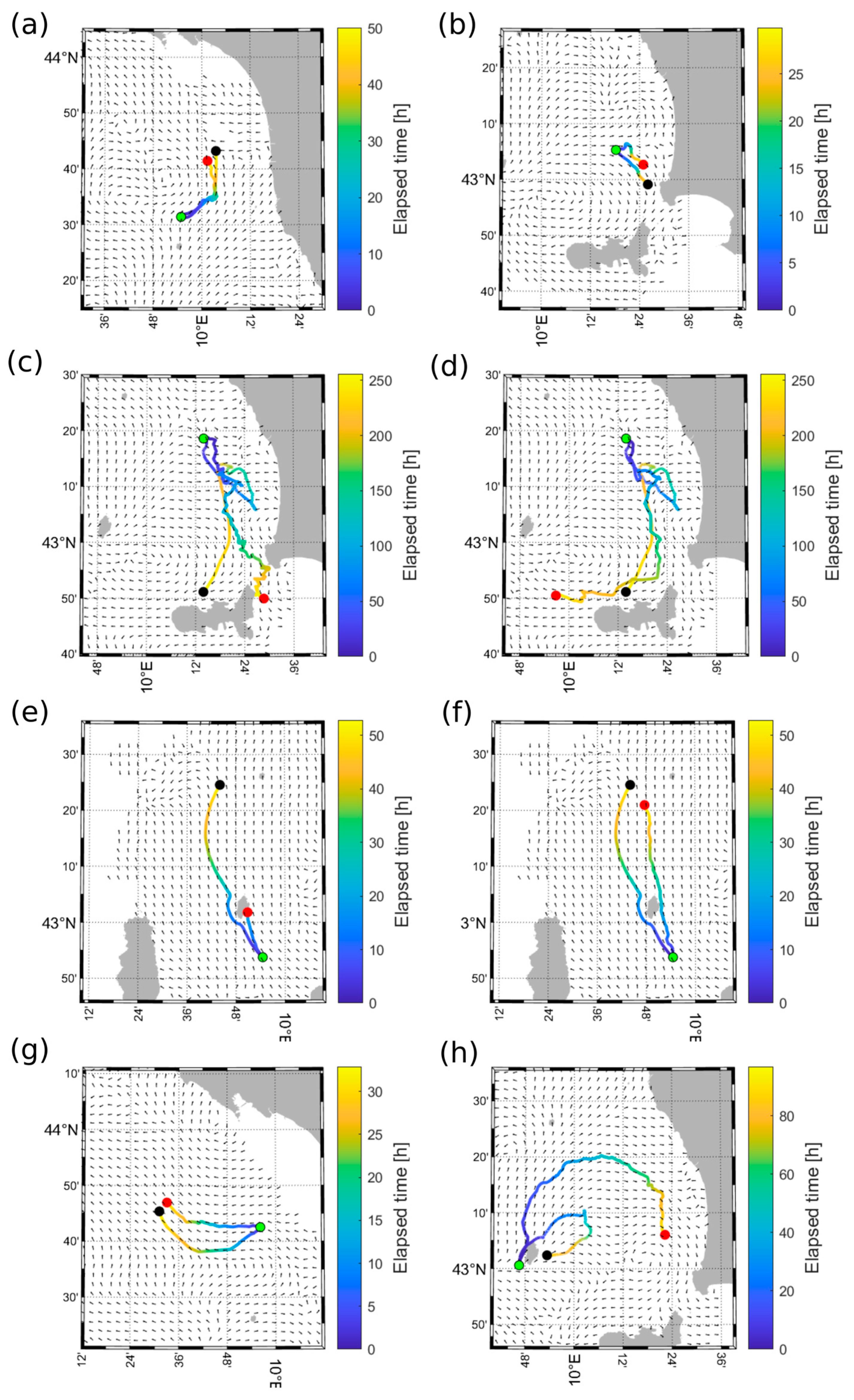
2.6. Comparison of Trajectories (Lagrangian Approach)

Drifter trajectories were also compared to those obtained from the simulation of virtual elements driven by the HF radar-derived currents.

Virtual drifter trajectories were integrated using the GNOME model [39], employing a 4th-order Runge–Kutta scheme, with no additional dispersion due to unresolved processes. Since the virtual drifters travel within the limited domain covered by the HF radar, we first identified an appropriate “footprint” or polygon representing this area.

Below is a description of the method used. The boundary function uses the geographical coordinates (latitude and longitude) of valid points to calculate the contour of the radar area, returning a polygon that represents the radar coverage. The shrink factor (sf) parameter controls the compactness of the contour. With sf = 0, a convex hull is obtained that may include external areas not covered by the radar, while higher sf values (up to 1) make the contour adhere more closely to the actual points, excluding areas without data. The extraction process is iterated up to four times to generate contours with different levels of compactness, which are saved and, if necessary, visualized. Since the radar coverage area may vary, a sufficiently representative area is selected for the period of interest. Figure 2a illustrates the radar field, while Figure 2b displays the ’radar footprint’ extracted as a result of the previously described procedure. Figure 3 presents the sub-trajectories extracted as a result of the previously described procedure.

More than one contour can be extracted from the procedure, based on the amount of data included within the footprint. The larger the area, the higher the probability of including erroneous data corrupted by noise, generally located at the boundaries, due to the distance from the antenna or the vicinity of the coastline. On the contrary, a smaller area has less data to perform the simulations. In our case, the second contour (the blue one) has been chosen as the limit boundary of the radar area, resulting in a good compromise between the elimination of corrupted data and the restriction of the useful area. With this procedure, only drifters that are within the selected radar boundary can be marked as ‘valid’.

We generally recommend using this procedure whenever working with radar data, as major issues often occur in the farthest regions or near the edges of the radar coverage area.

To address gaps in the HF radar data, different strategies were applied based on their duration. If data gaps exceeded 3 h, virtual trajectories were interrupted and reinitialized on the corresponding real trajectory at the first available time, whereas for shorter gaps, the velocities were linearly interpolated. Following this approach, approximately 90 sub-tracks were obtained from 26 different drifters, with each drifter remaining within radar coverage for an average of 4 days, reaching a maximum of 13 days (

Table 2. Summary table on the extraction of drifter sub-tracks. The first row shows the total number of drifters within the HF radar coverage area, while the second row reports the uniformly extracted 12 h sub-tracks.

Sub-Track Extracted	Mean Interval [Days]	Min. Interval [Days]	Max. Interval [Days]
88	4.2	1.01	12.96
705	12	12	12

, first row). It is to be noted that the number of drifters considered in this analysis is lower than the total (32), as some drifters got beached immediately after a few hours. To ensure a homogeneous analysis, drifter trajectories were segmented into uniform 12 h sub-tracks, a choice that balances the ability to capture both long-term trends and short-term variations while remaining suitable for different flow conditions. However, in regions with strong velocity gradients, shorter sub-trajectories or adaptive segmentation based on velocity changes may better resolve the complexity of the flow. High-variability areas, where currents shift significantly over small spatial or temporal scales, benefit from finer segmentation to capture localized phenomena such as eddies or wind-driven currents. Conversely, in more homogeneous regions with slower variations, longer trajectories effectively represent broader trends, such as tidal cycles or persistent flow patterns.

With position data recorded approximately every 5 min, resulting in about 103 samples per drifter, the 12 h trajectory framework provides a balance between dataset manageability and sufficient resolution to analyze both large-scale flow changes and short-term fluctuations. This duration also facilitates direct comparisons between real and virtual drifter trajectories while allowing flexibility in more dynamic flow regions. Although alternative approaches, such as further trajectory segmentation or adaptive methods, could refine the analysis in highly variable areas, the 12 h framework remains a robust and versatile choice for this study. A summary of the dataset is provided in Table 2 (second row).

3. Results and Discussion from Eulerian Comparison

3.1. HF Radials Comparison and QA

The comparison between the velocity derived from the drifter trajectory, projected onto the radial direction Ud, and the radial velocity measured by radars, Ur, is reported in Figure 3 as scatter plots for the three HF radar systems. The TINO system performs better than LIVO and SVIN, as confirmed by the root mean squared error (RMSE) and the Pearson correlation coefficient (ρ) reported in

Table 3. Summary of the statistics from the comparison between Ud and Ur.

HF Radar	RMSE [m/s]	ρ [-]
TINO	0.10	0.85
TINO (filtered)	0.10	0.89
LIVO	0.14	0.53
LIVO (filtered)	0.10	0.76
SVIN	0.15	0.37
SVIN (Kriging)	0.14	0.43

.

A further improvement in the agreement between Ur and Ud can be obtained if some of the radial data are filtered out based on the distance from the antenna (range), the bearing, and the time of the day. For the TINO HF radar, in case we take only data in the range 10–50 km and measured between 8:00 PM to 8:00 AM (night time), this reaches 0.89, and the linear fit is almost equal to the 1:1 line (Table 3). Similarly, if we take data in the range 10–40 km and bearing 190–315° for the LIVO HF radar, we obtain RMSE = 0.1 m/s, ρ = 0.76. However, for the SVIN HF radar, we did not find a combination of filters able to improve the results.

In the case of the SVIN station, the introduction of the Kriging method, as detailed in the previous section, led to a modest improvement. The correlation between currents measured by the drifters and those recorded by the HF radar at the SVIN station increased from 0.37 to 0.43.

In contrast, no significant improvement was observed in the Livorno area, while a slight decrease in correlation was noted for the northern TINO area, dropping from 0.85 to 0.84. These findings align with the characteristics of the method, which is better suited for capturing local variations, although improvements can be constrained by factors such as the choice of covariance model (which can be challenging to estimate), data density, and the complexity of the flow field.

While Kriging remains effective in regions with high spatial variability, its performance can be more limited in uniform flow conditions, where minor fluctuations may be overemphasized, potentially leading to small biases. One possible way to address this limitation is the implementation of an adaptive parameter adjustment mechanism, where variogram parameters are dynamically tuned based on local flow characteristics. However, such an approach requires careful calibration to avoid instability or loss of spatial coherence in the velocity estimates. Future studies could investigate the integration of adaptive Kriging techniques or hybrid interpolation methods to improve the method’s robustness across different flow regimes.

Despite these challenges, Kriging remains a valuable tool for improving velocity estimates, particularly in complex flow fields. The method’s ability to account for spatial correlations and local fluctuations demonstrates its utility, though careful parameter selection and validation remain crucial for maximizing its effectiveness under different environmental conditions.

Diagnostic metrics (e.g., XARW) and data-filtering techniques (e.g., VART_QC and MDFL_QC thresholds) were employed to identify and isolate the systematic errors arising from radar hardware or environmental interferences. Despite this improvement, the SVIN antenna exhibited the poorest performance. To determine if environmental interference could be the cause, an APM (antenna pattern measurement), which serves as a form of calibration, was conducted. The new pattern was applied to the radar, and the data were reprocessed. However, the results showed little if any improvement in terms of correlation and in terms of average differences calculated along the trace.

We examined the radar performance during distinct periods, such as analyzing data from the SVIN radar before and after observed hardware malfunctions, to differentiate environmental influences from system-related issues.

To identify system-related issues, a thorough analysis of the diagnostic parameters was conducted. Benchmark values derived from both the manufacturer’s recommendations and from similar SeaSonde radar installations [3,40] were compared with the averaged values from each station during the period of interest. We found that the XARW (amount of the transmitted signal returning toward the transmitter) was larger than expected for the SVIN antenna, reaching the limit value (5 w) in about 30% of cases, probably due to an imperfect coupling between the antenna and the transmission system. For the TINO antenna, the XARW was equal to zero in most cases, while for the LIVO system, it is always less than 2 w. Excluding radar values where the parameter XARW was above the 2 w threshold, the obtained correlation values increased from 0.37 to 0.47 and 0.55 if the XARW was lower than 2 w and strictly lower than 2 w, respectively (Figure 4a, Figure 4b). Even the RMSE was reduced after this filter was applied (

Table 4. Summary of the statistics from the comparison shown in Figure 4.

HF Radar	RMSE [m/s]	ρ [-]
SVIN (thr < 2 w)	0.14	0.47
SVIN (thr ≤ 2 w)	0.13	0.55

).

To verify the correct functioning of the SVIN radar during different periods, the Eulerian velocities from the CHARTE drifters, provided by IFREMER and related to May–Sep 2019 (Figure 1c), were compared with SVIN and LIVO radial velocities (Figure 5) for a time window when the XARW values for the SVIN system were normal.

Although these are different drifters, but with similar performances in regard to surface current measurements, we observe that the correlation values for SVIN are larger than those in Figure 3c (when the XARW values were out of the normal range). This correlation is even better than that of the Livorno antenna in the same period (Figure 5a), which also showed improved performances with respect to Figure 3b. Despite this result, which can be affected by the type of drifters, we obtained a confirmation of the good quality of the SVIN data before the failure.

The scatter plot between TINO25 radials (operating at 25 MHz) and the Eulerian velocities from CODE drifters was also made (Figure 6a). TINO25 is located in the same position as TINO, and the sea sectors illuminated by radars have a large overlapping area. Differences lie in the range and spatial resolution, as TINO25 has a range of 40 km and 1 km resolution, and TINO has an 80 km range and a 1.5 km resolution. The comparison of two radars is useful for understanding whether there is any positive effect linked to the higher resolution in an area close to the coast on the overall data quality.

By comparing the scatter plots Figure 3a and Figure 6a, we observed that TINO25 shows a lower correlation value with respect to TINO, specifically 0.68 and 0.84, respectively.

A possible explanation could attribute this difference in performance to different hardware and software characteristics, as the hardware equipment used by TINO25 is some years older than that of TINO, which is also an upgrade of the previous radar version. The obtained correlations are consistent with previous studies conducted in the Mediterranean Sea. For example, [14] radar data in the Malta–Sicily Channel were validated using drifters and ADCP data. The reported correlation coefficients for the zonal and meridional velocity components between the radar and drifters ranged from 0.4 to 0.94, and the corresponding RMSE was between 0.09 and 0.14 m/s. In [41], where the HF radar systems (operating between 13.5–25 MHz) were deployed across five different Mediterranean sites, the obtained RMSEs for the radial velocities and drifter-derived velocities ranged from 0.05 to 0.16 m/s. These studies emphasize that the results are strongly influenced by local environmental factors, such as radio-frequency interference, vertical shear, and site-specific dynamics, leading to broad variability between stations. This is consistent with our observations, particularly in regions with more complex flow patterns. Furthermore, our findings are consistent with those of [12] in the Gulf of La Spezia, which is near our study area, where a strong agreement between radar and drifter data was observed. In this case, the correlation coefficients ranged from 0.66 to 0.87, with RMSE values between 5.2 cm/s and 4.55 cm/s. The strong agreement observed in this study, along with the low RMSE, is attributed to factors such as high spatial resolution (250 m) and the robust performance of the WERA radar system. Similarly, in other studies (conducted in different areas), such as that by [16], the radial data from the CODAR radar (at 13.5 and 25 MHz) were compared with the drifter trajectories, yielding RMSE values around 10 cm/s and a correlation coefficient of 0.84. Comparable results are also observed in the work of [42], conducted in Northern Norway.

3.2. QC Procedures and Calibration

Data acquired by the HF radar system were also checked in relation to the QC procedures established by the European best practices for QA/QC [11]. Prescribed thresholds depend on each radar area and should not be considered fixed: the higher the variability of currents (velocity and direction), the higher the threshold values to be adopted. For the SLS, typical current velocities are normally in the range between 0.1 and 0.4 m/s, and we expect benefits from setting the QC parameters accordingly.

In Figure 7a, we show that the correlation increases when using more restrictive values for the VART_QC threshold. Lowering the VART_QC parameter from 1 to 0.5 m/s results in an increase in correlation for LIVO of about 5%, with a data loss of approximately 1%. Smaller improvements are observed for the SVIN and TINO radars. In general, setting VART_QC to 0.5 m/s represents a reasonable trade-off between data retention and improved radar performance in terms of correlation.

A similar analysis was conducted for MDFL_QC (Figure 7c,d). However, the results indicate that modifying MDFL_QC does not lead to significant additional improvements beyond those obtained by tuning VART_QC alone. Further tests, including cases where high VART_QC values were combined with low MDFL_QC values, confirmed that no synergistic effects exist between these parameters. Therefore, we conclude that optimizing VART_QC alone is sufficient to enhance correlation, while adjusting MDFL_QC does not provide additional benefits.

For the RDCT_QC flag, we verified that values below the default threshold (200) lead to an increase in correlation, whereas higher values do not yield further improvements. The CSPD_QC threshold (set at 1.2 m/s) was not tested in this study, as lowering it could lead to the exclusion of “false positive” events in the presence of extreme conditions. Although this default value is relatively high for the study area, it remains appropriate for capturing occasional strong currents.

From a practical standpoint, tuning QC flag parameters allows for an improvement in correlation of approximately 5%, at the cost of discarding a small fraction of data. A good climatology of the circulation patterns in a given area can help refine the selection of these thresholds.

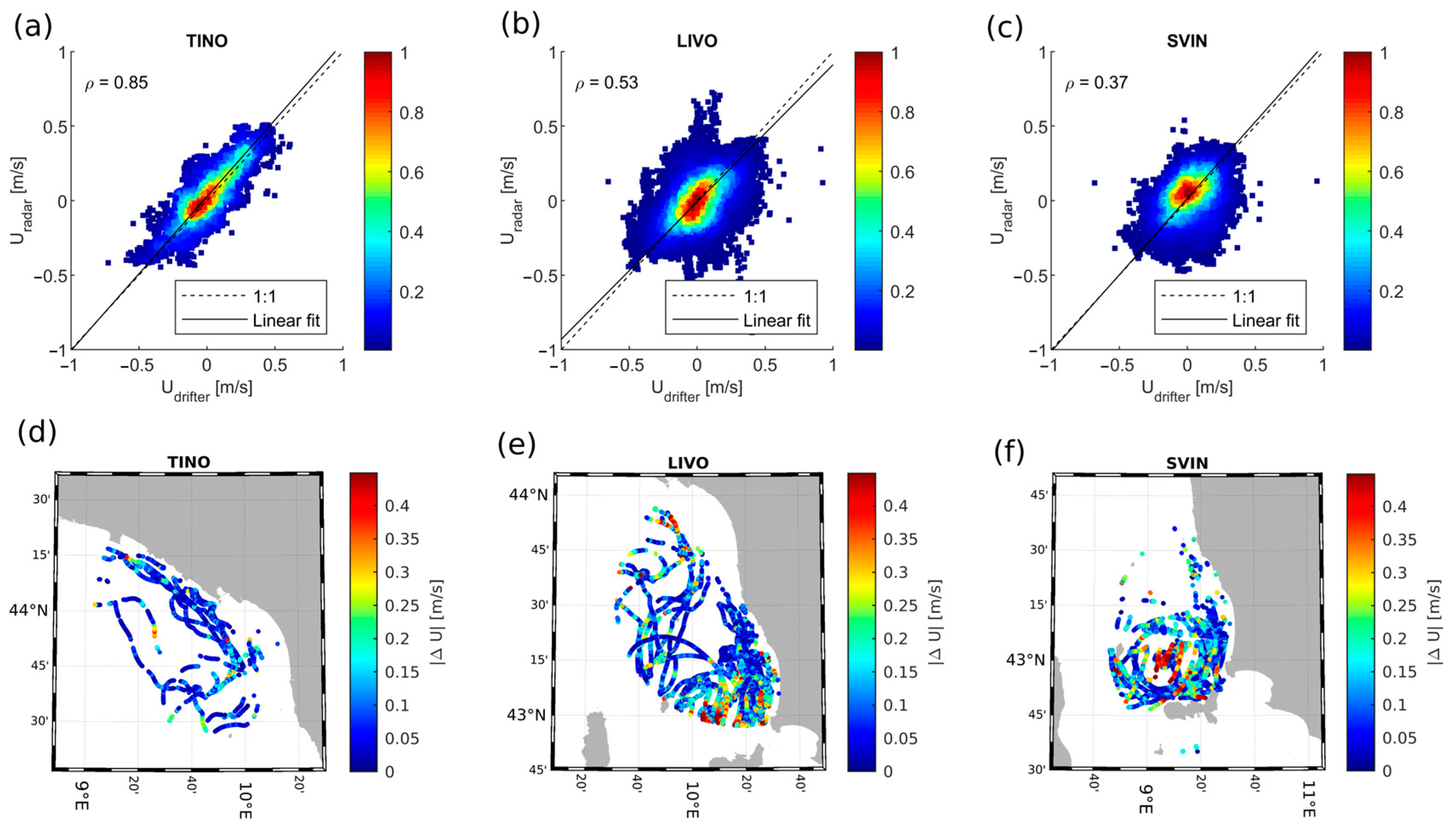
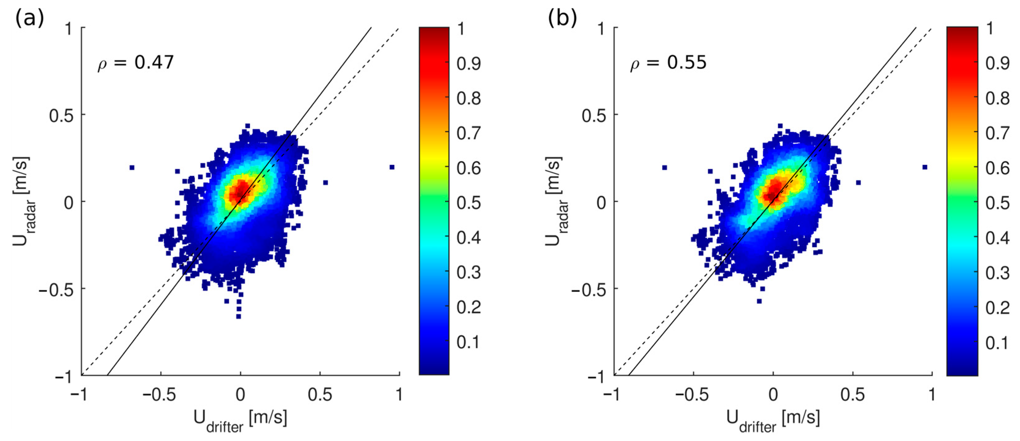
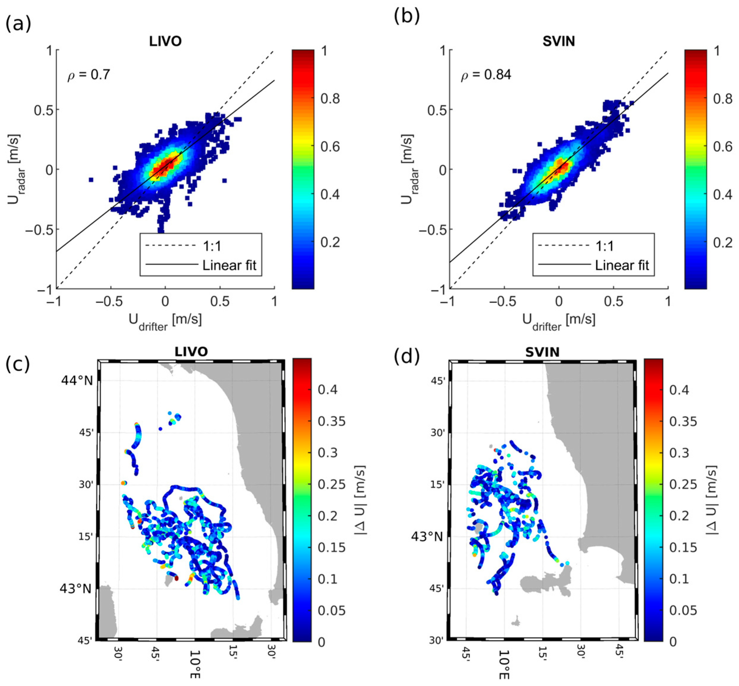
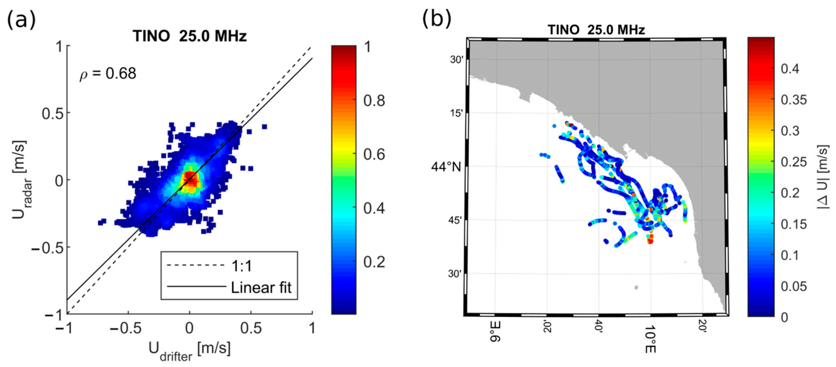
3.3. Baseline Velocity Comparison

To identify the presence of a radar bearing offset, it is possible to use a radar-to-radar comparison technique [43,44,45,46], where a pair of radars is found on the overwater baseline or at the same transmission point. Radial velocity from the two radars, observed at half distance along the overwater baseline, must be equal and of the opposite sign (or equal when antennas are co-located). Otherwise, the best match is sought by considering the radial data of the two radars with different bearing angles.

In the present analysis, the bearing offset angle varies from −15° to +15°. The conformation of the Tuscan Archipelago coastline allows us to apply this technique to SVIN and LIVO (Figure 8b) or for the co-located TINO and TINO25 (Figure 8a).

Table 5. Table of possible correlations by crossing the radials of LIVO and SVIN, as the selected bearing angle varies. The value highlighted in red is the one corresponding to the correlation in the points without offset. The one in green is the optimal value found, which corresponds to an offset of 10° for SVIN and 25° for LIVO.

	SVIN
		R1 (−15°)	R2 (−10°)	R3 (−5°)	R4 (0°)	R5 (+5°)
LIVO	R3 (−5°)	0.24	0.53	0.57	0.24	0.33
	R4 (0°)	0.27	0.37	0.33	0.36	0.04
	R5 (+5°)	0.63	0.69	0.66	0.60	0.17
	R6 (10°)	0.55	0.67	0.61	0.48	0.20
	R7 (+15°)	0.31	0.60	0.47	0.22	0.19

reports the ρ values from the reciprocal comparison between LIVO and SVIN, for which the best matching point is obtained by selecting an offset of 5° and 10°, respectively. Discrepancies of this type are quite common for SeaSonde-type radars and may depend on local pattern distortion, on the low signal-to-noise ratio (higher if the radials are closer to the shoreline), or on the performance of the MUSIC (MUltiple Signal Identification and Classification) algorithm [37], used to reconstruct the direction of the radials. Furthermore, the issue cannot be resolved by rotating the entire radial velocity data, as by its nature, it is not uniformly distributed in space [47].

Regarding the two radars at Tino, the bearing offset was calculated at three distinct points located 18 km away (approximately half of the maximum range measurable by TINO25) and spaced 45° apart. It has been observed that, in the 225° direction, there is a bearing offset of about 10° for both radars, while in the other directions, this offset is not detectable. This confirms that the bearing offset is not spatially uniform. The low quality of the signal in this sector is also confirmed by the correlation value, which, in the 225° direction, is lower and equal to about 0.54, while ρ = 0.85 at 270° and ρ = 0.73 at 180°.

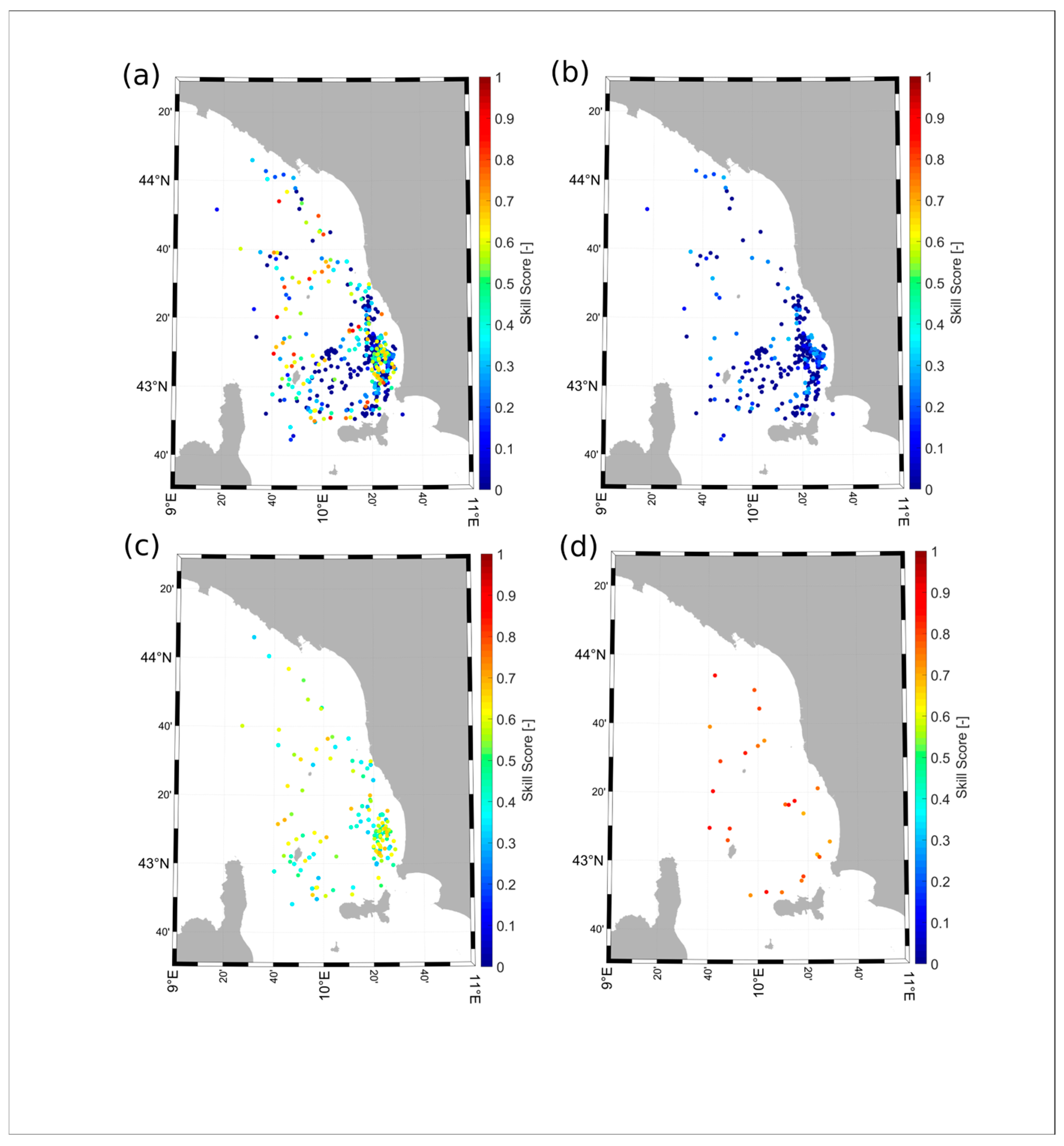
4. Results and Discussion from Lagrangian Comparison

For virtual drifters released in areas where the currents are more uniform, the distance from real drifters does not increase significantly over time (Figure 9a,b,g). In other cases, small random variations in the initial conditions can lead to completely different outcomes. For instance, Figure 9c shows how a virtual drifter behaves differently near the Piombino Channel, where it crosses the channel, while in Figure 9d, the drifter continues its trajectory westward.

Similarly, Figure 9e illustrates how the presence of the island of Capraia can influence the trajectories. Being downstream of the mean current, the island can amplify small divergences present at the initial stages of the compared trajectories and act as an obstacle. In particular, the virtual drifter’s trajectory is interrupted by the island, whereas in Figure 9f, a slight variation in the starting position leads to a completely different outcome, allowing the drifter to bypass the obstacle.

These discrepancies can also arise from gaps in radar data due to the shape of the coastline or signal loss in specific radar cells. In such cases, the comparison was limited to the useful sub-tracks only. Finally, Figure 9h highlights the difficulty in capturing strong flow gradients due to the limited resolution of the HF radar. The presence of an anticyclonic vortex, detectable through the real drifter’s trajectory, is only partially captured by the radar data. This is primarily due to the radar’s inability to resolve small-scale current features, which cause the real drifter to follow a trajectory with a smaller radius of curvature [48].

In general, the quantification of these discrepancies is challenging. One possible approach is to describe stochastic processes operating at minute scales upon small drifting objects, a phenomenon extensively explored in the existing literature (e.g., [44,49,50]). This phenomenon accounts for instances where slight variations in the initial positions of real and virtual drifters occasionally lead to substantial disparities in their final locations, which is evident in some of the above-shown trajectories. A summary of the temporal evolution of the divergence for all the trajectories is reported in Figure 10. The maximum divergence after 12 h can reach about 25 km distance. However, the 90th percentile corresponds to a separation distance around 10 km between virtual and real drifters, while the mean is around 5 km, similarly to [13,20], although an analogous experiment carried out in the Gulf of La Spezia [12] with repeated launches of small clusters of drifters (3–6 units) showed lower values of separation distance, probably due to the higher resolution of the radar system (operating at 45 MHz) and a more uniform circulation.

A more adequate metric with respect to the separation distance is based on the cumulative Lagrangian separation distances normalized by the associated cumulative trajectory lengths [51]. This skill score can be used to map its spatial distribution to have a global view of radar performance across the entire monitoring area.

$$s={\displaystyle \frac{\sum _{i=1}^N{d}_i}{\sum _{i=1}^N{L}_i}}$$

(4)

The skill scores are calculated according to Formula (4):

SS = 1-s (s ≤ 1); 0 (s > 1), where N is the number of time steps from the start of the simulation for the entire observation interval, Li is the length of the trajectory observed at the i-th time step, and di is the distance at each time step between the position of the observed drifter and that simulated.

The skill score (SS), as defined here, ranges from zero (no skill) to one (perfect simulation). The results of this calculation are shown in Figure 11, with different skill score thresholds for better clarity. The skill scores are calculated at each time step (roughly 5 min) over 12 h simulations, considering all drifters in the area and across all simulation days. The overall mean ss value, which is 0.24, is relatively low, as is typical in this type of analysis. As anticipated, the lowest skill scores (SS < 0.3) are predominantly found in the Southeast Ligurian Sea, particularly in the shelf area near the coast. This region is characterized by weaker currents, larger horizontal velocity shear, and frequent small vortices (as seen in [29]). On the other hand, the highest skill scores (SS > 0.7) are mainly observed in deeper sea areas, especially along the edge of the Tuscany Archipelago platform. Here, the North Mediterranean current from the Corsica Channel dominates, and the flow is generally more uniform and energetic.

5. Conclusions

This study focused on validating the LaMMA Consortium’s radar network along the Tuscan coast using both Eulerian and Lagrangian methodologies. These systems are complex to manage but provide an extraordinary amount of observational data, supporting various marine-monitoring needs.

From a Eulerian perspective, we analyzed the radial velocity components from each radar station separately, comparing them to the drifter-derived velocities projected along radial directions. Conversely, the Lagrangian approach allowed us to assess the overall system performance by comparing the trajectories of virtual drifters, driven by total velocities, against those of real drifters. Eulerian comparisons for the LIVO and TINO radars yielded results consistent with previous studies in the Mediterranean Sea ([12,14,16,41,42]), with correlation values ranging from 0.53 to 0.89 and RMSE between 0.1 m/s and 0.14 m/s, depending on whether the data were filtered or unfiltered, respectively. For SVIN, the correlation values were between 0.47 and 0.55 (RMSE = 0.13–0.14 m/s) after filtering the reflected signal in transmission (XARW less than or equal to 2 w). Adjusting the quality control parameters proved effective in enhancing radar data quality, although for regular checks and validation, the use of CODE drifters was essential.

About ten QA parameters and four QC parameters were used for studying the quality of the radar signal, before and after the processing phases. This analysis helped identify a possible cause of radar malfunction and contributed to the fine-tuning of output generation procedures by adjusting specific parameters (e.g., modifying the VART_QC value), leading to improvements in correlation.

As a further improvement for areas with high spatial variability, the Kriging method for velocity interpolation was tested. This approach led to some slight improvements for the SVIN station, where the correlation between currents measured by drifters and those recorded by the HF radar increased from 0.37 to 0.43. However, no improvement was observed in the Livorno area or at TINO, where there was even a slight decrease. This suggests that, while Kriging effectively captures local variations, it may not provide significant benefits when data variability is limited, and its added complexity may not justify its use.

Additional investigations involving CARTHE drifters helped confirm the quality of the radar data. In particular, this was observed for the SVIN radar during a period when it had no operational anomalies, as well as for the LIVO radar.

The comparison of two radars co-located on Isola del Tino, operating at different frequencies (13.5 MHz for TINO and 25 MHz for TINO25), did not indicate a superior performance of the higher-resolution radar in measuring the radial drifter speed. A Eulerian analysis, performed using the same drifters with both radars, yielded correlation values of 0.84 for the 13.5 MHz radar and 0.68 for the 25 MHz radar. The reasons for this unexpected behavior remain unclear and could be attributed to various factors, including the older age of the 25 MHz radar system, electromagnetic interference, or other unidentified causes.

As a further analysis, the ’Bearing Offset’ technique was used to quantify the deformation of the radar field wherever the coastal features allowed. In the southern region, for the LIVO and SVIN pair, deviations of up to 25° and 10°, respectively, were observed. In the northern region, no offset was detected in the 270° and 180° sectors for the TINO area, while a similar offset of approximately 10° was noted in the 225° sector for both TINO and TINO25, indicating that these two radars respond in a similar way to the distortion of the electromagnetic field. The presence of this offset is challenging to explain. In general, if the beam offset at a specific angle is consistent for both radars operating at different frequencies, it suggests that the primary cause is not related to propagation factors that typically vary with frequency, such as atmospheric refraction or ionospheric or geomagnetic effects. Instead, it is likely due to factors common to both frequencies. In this study, we hypothesize that the beam offset results from the interaction between the electromagnetic field and the local environment (e.g., coastal features and obstacles), leading to reflection patterns or disturbances that similarly affect both radars.

The comparison of real and virtual drifters (Lagrangian analysis) showed that, for this particular environment, slight inaccuracies in the HF-derived surface velocity field can cause considerable divergence in the final positions, especially due to many submesoscale features, also produced by the presence of several islands, which are unlikely detected by the radars. The average deviations of the virtual particles from the real ones were approximately 25 km after 12 h. The overall mean skill score (SS) value was equal to 0.24. Lower skill scores were found mostly in the Southeastern Ligurian Sea, in the shelf area closer to the coast. Where the currents were weaker, the horizontal velocity shear was generally larger, and small vortices were frequent. Higher skill scores (SS > 0.7) were mainly observed in deep marine areas, where the flow was more uniform and dominated by mesoscale features.

We also highlight that, although local in scope, this study can be extended to numerous regions monitored by HF radar, particularly those characterized by high variability in current flows. The proposed methodological approach is universally applicable to HF radar systems. For example, the radar data fine-tuning technique can be applied to all HF radar systems. The antenna footprint technique, which helps identify areas less prone to measurement errors, is recommended for radar data analysis. The evaluation of QA threshold compliance should always be performed, especially when values are close to the threshold, even if the radar-derived current patterns appear consistent and realistic. Furthermore, in areas with high variability, where radar measurements may be less reliable, particularly at lower frequencies, and where errors can be significant, more advanced interpolation techniques, such as Kriging, are recommended to enhance current representation using drifter data.

Lastly, we note that future research should focus on fine-tuning the radar frequency settings and potentially developing adaptive radar systems tailored to specific environmental conditions.

References

1. Reyes, E.; Aguiar, E.; Bendoni, M.; Berta, M.; Brandini, C.; Cáceres-Euse, A.; Capodici, F.; Cardin, V.; Cianelli, D.; Ciraolo, G.; et al. Coastal high-frequency radars in the Mediterranean–Part 2: Applications in support of science priorities and societal needs. Ocean Sci. 2022, 18, 797–837. [Google Scholar] [CrossRef]
2. Lorente, P.; Aguiar, E.; Bendoni, M.; Berta, M.; Brandini, C.; Cáceres-Euse, A.; Capodici, F.; Cianelli, D.; Ciraolo, G.; Corgnati, L.; et al. Coastal high-frequency radars in the Mediterranean–Part 1: Status of operations and a framework for future development. Ocean Sci. 2022, 18, 761–795. [Google Scholar] [CrossRef]
3. Cook, T.; Hazard, L.; Otero, M.; Zelenke, B. Deployment and Maintenance of a High-Frequency Radar (HFR) for Ocean Surface Current Mapping: Best Practices; University of California San Diego, Scripps Institution of Oceanography for SCCOOS: San Diego, CA, USA, 2008. [Google Scholar] [CrossRef]
4. Horstmann, J.; Corgnati, L.; Mantovani, C.; Quentin, C.; Reyes, E.; Rubio, A.; del Rio, J.; Berry, A. Report on Best Practice in the Implementation and Use of New Systems in JERICO-RI. Part 1: HF-Radar Systems and Part 2: Cabled Coastal Observatories; WP2, Deliverable 2.4. Version 1.0; IFREMER for JERICO NEXT: Brest, France, 2019. [Google Scholar] [CrossRef]
5. Mantovani, C.; Corgnati, L.; Horstmann, J.; Rubio, A.; Reyes, E.; Quentin, C.; Cosoli, S.; Asensio, J.L.; Mader, J.; Griffa, A. Best Practices on High Frequency Radar Deployment and Operation for Ocean Current Measurement. Front. Mar. Sci. 2020, 7, 210. [Google Scholar] [CrossRef]
6. Chapman, R.D.; Shay, L.K.; Graber, H.C.; Edson, J.B.; Karachintsev, A.; Trump, C.L.; Ross, D.B. On the accuracy of HF radar surface current measurements: Intercomparisons with ship-based sensors. J. Geophys. Res. 1997, 102, 18737–18748. [Google Scholar] [CrossRef]
7. Teague, C.C.; Vesecky, J.F.; Hallock, Z.R. A comparison of multifrequency HF radar and ADCP measurements of near-surface currents during COPE-3. IEEE J. Ocean Eng. 2001, 26, 399–405. [Google Scholar] [CrossRef]
8. Liu, Y.; Weisberg, R.H.; Merz, C.R. Assessment of CODAR SeaSonde and WERA HF radars in mapping surface currents on the West Florida Shelf. J. Atmos. Ocean. Technol. 2014, 31, 1363–1382. [Google Scholar] [CrossRef]
9. Jimenez, P.; Piedracoba, S.; Fanjul, E.A. Validation of high-frequency radar ocean surface current observations in the NW of the Iberian Peninsula. Cont. Shelf Res. 2015, 92, 1–15. [Google Scholar] [CrossRef]
10. Wei, G.; He, Z.; Xie, Y.; Shang, S.; Dai, H.; Wu, J.; Liu, K.; Lin, R.; Wan, Y.; Lin, H.; et al. Assessment of HF radar in mapping surface currents under different sea states. J. Atmos. Ocean. Technol. 2020, 37, 1403–1422. [Google Scholar] [CrossRef]
11. Ohlmann, J.C.; Niiler, P.P. Circulation over the continental shelf in the northern Gulf of Mexico. Prog. Oceanogr. 2005, 64, 45–81. [Google Scholar] [CrossRef]
12. Molcard, A.; Poulain, P.-M.; Forget, P.; Griffa, A.; Barbin, Y.; Gaggelli, J.; Maistre, J.; Michel, R. Comparison between VHF radar observations and data from drifter clusters in the Gulf of La Spezia (Mediterranean Sea). J. Mar. Syst. 2009, 78, S79–S89. [Google Scholar] [CrossRef]
13. Kalampokis, A.; Uttieri, M.; Poulain, P.-M.; Zambianchi, E. Validation of HF Radar-Derived Currents in the Gulf of Naples with Lagrangian Data. IEEE Trans. Geosci. Remote Sens. 2016, 13, 1452–1456. [Google Scholar] [CrossRef]
14. Capodici, F.; Cosoli, S.; Ciraolo, G.; Nasello, C.; Maltese, A.; Poulain, P.; Drago, A.; Azzopardi, J.; Gauci, A. Validation of HF radar sea surface currents in the Malta-Sicily Channel. Remote Sens. Environ. 2019, 225, 65–76. [Google Scholar] [CrossRef]
15. Corgnati, L.; Mantovani, C.; Griffa, A.; Berta, M.; Penna, P.; Celentano, P.; Bellomo, L.; Carlson, D.F.; D’Adamo, R. Implementation and Validation of the ISMAR High-Frequency Coastal Radar Network in the Gulf of Manfredonia (Mediterranean Sea). IEEE J. Ocean. Eng. 2019, 44, 424–445. [Google Scholar] [CrossRef]
16. Ohlmann, C.; White, P.; Washburn, L.; Emery, B.; Terrill, E.; Otero, M. Interpretation of Coastal HF Radar Derived Surface Currents with High-Resolution Drifter Data. J. Atmos. Ocean. Technol. 2007, 24, 666–680. [Google Scholar] [CrossRef]
17. Davis, R.E. Drifter observations of coastal surface currents during CODE: The method and descriptive view. J. Geophys. Res. 1985, 90, 4741–4755. [Google Scholar] [CrossRef]
18. Stewart, R.H.; Joy, J.W. HF radio measurements of surface currents. Deep Sea Res. I 1974, 21, 1039–1049. [Google Scholar]
19. Astraldi, M.; Gasparini, G.P.; Manzella, G.M.R.; Hopkins, T.S. Temporal Variability of Currents in the Eastern Ligurian Sea. J. Geophys. Res. 1990, 95, 1515–1522. [Google Scholar] [CrossRef]
20. Artale, V.; Astraldi, M.; Buffoni, G.; Gasparini, G.P. Seasonal variability of gyre-scale circulation in the Northern Tyrrhenian Sea. J. Geophys. Res. 1994, 99, 14127–14138. [Google Scholar] [CrossRef]
21. Astraldi, M.; Bianchi, C.N.; Gasparini, G.P.; Morri, C. Climatic fluctuations, current variability and marine species distribution—A case-study in the Ligurian Sea (north-west Mediterranean). Oceanol. Acta 1995, 18, 139–149. [Google Scholar]
22. Sciascia, R.; Magaldi, M.G.; Vetrano, A. Current reversal and associated variability within the Corsica Channel: The 2004 case study. Deep Sea Res. I 2019, 144, 39–51. [Google Scholar] [CrossRef]
23. Iacono, R.; Napolitano, E. Aspects of the summer circulation in the eastern Ligurian Sea. Deep Sea Res. I 2020, 166, 103407. [Google Scholar]
24. Copernicus Marine Environmental Monitoring Service (CMEMS). QA Best Practices and Protocols on QC for Radial and Total HF Radar Data (INCREASE WP3, D3.1); Copernicus Marine Environmental Monitoring Service (CMEMS)/Mercator Ocean: Ramonville Saint-Agne, France, 2017. [Google Scholar]
25. CNR-ISMAR HF Radar Network. Available online: http://radarhf.ismar.cnr.it/OperatingNetwork.html (accessed on 22 November 2023).
26. THREDDS Data Server-European High Frequency Radar Node. Available online: http://150.145.136.27:8080/thredds/HF_RADAR/HFradar_catalog.html (accessed on 22 November 2023).
27. Bushnell, M.; Worthington, H. Manual for Real-Time Quality Control of High Frequency Radar Surface Current Data: A Guide to Quality Control and Quality Assurance for High Frequency Radar Surface Current Observations, Version 2.0; IOOS: Silver Spring, MD, USA, 2022; pp. 1–57. [Google Scholar]
28. Cosoli, S.; Bolzon, G. A real-time and offline quality control methodology for SeaSonde high-frequency radar currents. J. Atmos. Ocean. Technol. 2012, 29, 1313–1328. [Google Scholar] [CrossRef]
29. Cosoli, S.; Grcic, B. Quality Control Procedures for IMOS Ocean Radar Manual Version 2.1; Integrated Marine Observing System: Hobart, Australia, 2019. [Google Scholar] [CrossRef]
30. Poulain, P.-M. Demonstration Experiment and Design of Network for Oceanographic and Acoustic Measurements; Memorandum Report CMRE-MR-2020-17; NATO-STO CMRE: La Spezia, Italy, 2020; p. 43. [Google Scholar]
31. Poulain, P.-M.; Gerin, R.; Mauri, E.; Pennel, R. Wind Effects on Drogued and Undrogued Drifters in the Eastern Mediterranean. J. Atmos. Ocean. Technol. 2009, 26, 1144–1156. [Google Scholar] [CrossRef]
32. Poulain, P.-M.; Gerin, R. Assessment of the Water-Following Capabilities of CODE Drifters Based on Direct Relative Flow Measurements. J. Atmos. Ocean. Technol. 2019, 36, 621–633. [Google Scholar] [CrossRef]
33. Pacific Gyre Drifting Buoys. Available online: https://www.pacificgyre.com (accessed on 22 November 2023).
34. Novelli, G.; Guigand, C.M.; Cousin, C.; Ryan, E.H.; Laxague, N.J.M.; Dai, H.; Haus, B.K.; Özgökmen, T.M. A Biodegradable Surface Drifter for Ocean Sampling on A Massive Scale. J. Atmos. Ocean. Technol. 2017, 34, 2509–2532. [Google Scholar] [CrossRef]
35. Poulain, P.-M.; Centurioni, L.; Özgökmen, T. Comparing the Currents Measured by CARTHE, CODE and SVP Drifters as a Function of Wind and Wave Conditions in the Southwestern Mediterranean Sea. Sensors 2022, 22, 353. [Google Scholar] [CrossRef] [PubMed]
36. Pawlowicz, R. “M_Map: A Mapping Package for MATLAB”, Version 1.4m, [Computer Software]. 2020. Available online: www.eoas.ubc.ca/~rich/map.html (accessed on 1 March 2025).
37. Allard, D.; Chilès, J.-P.; Delfiner, P. Geostatistics: Modeling Spatial Uncertainty. Math. Geosci. 2013, 45, 377–380. [Google Scholar] [CrossRef]
38. Cressie, N.A.C. Statistics for Spatial Data, Wiley Series in Probability and Statistics; John Wiley & Sons: New York, NY, USA, 1993; pp. 1–900. [Google Scholar] [CrossRef]
39. Beegle-Krause, C.J. General NOAA Oil Modeling Environment (GNOME): A New Spill Trajectory Model. In Proceedings of the IOSC 2001, Tampa, FL, USA, 26–29 March 2001; pp. 865–871. [Google Scholar] [CrossRef]
40. Emery, M.; Washburn, L. Evaluation of SeaSonde Hardware Diagnostic Parameters as Performance Metrics; NOAA: Silver Spring, MA, USA, 2007. [Google Scholar]
41. Bellomo, L.; Griffa, A.; Cosoli, S.; Falco, P.; Gerin, R.; Iermano, I.; Zervakis, V. Toward an Integrated HF Radar Network in the Mediterranean Sea to Improve Search and Rescue and Oil Spill Response: The TOSCA Project Experience. J. Oper. Oceanogr. 2015, 8, 95–107. [Google Scholar]
42. Röhrs, J.; Sperrevik, A.; Christensen, K.; Broström, G.; Breivik, Ø. Comparison of HF Radar Measurements with Eulerian and Lagrangian Surface Currents. Ocean Dyn. 2015, 65, 541–557. [Google Scholar] [CrossRef]
43. Lorente, P.; Piedracoba, S.; Soto-Navarro, J.; Alvarez-Fanjul, E. Evaluating the surface circulation in the Ebro delta (northeastern Spain) with quality-controlled high-frequency radar measurements. Ocean Sci. 2015, 11, 921–935. [Google Scholar] [CrossRef]
44. Paduan, J.; Kim, K.C.; Cook, M.S.; Chavez, F.P. Calibration and Validation of Direction-Finding High-Frequency Radar Ocean Surface Current Observations. IEEE J. Ocean. Eng. 2006, 31, 862–875. [Google Scholar] [CrossRef]
45. Yoshikawa, Y.; Masuda, A.; Marubayashi, K.; Ishibashi, M.; Okuno, A. On the accuracy of HF radar measurement in the Tsushima Strait. J. Geophys. Res. 2006, 111, C4. [Google Scholar] [CrossRef]
46. Atwater, P.; Heron, M. HF radar two-station baseline bisector comparisons of radial components. In Proceedings of the OCEANS’10 IEEE Sydney, Sydney, Australia, 24–28 May 2010; pp. 1–4. [Google Scholar] [CrossRef]
47. Laws, K.; Paduan, J.D.; Vesecky, J. Estimation and assessment of errors related to antenna pattern distortion in CODAR SeaSonde high-frequency radar ocean current measurements. J. Atmos. Ocean. Technol. 2010, 27, 1029–1043. [Google Scholar]
48. Cosoli, S.; Bolzon, G. Accuracy of surface current mapping from High-Frequency (HF) ocean radars. B. Geofis. Teor. Appl. 2015, 56, 55–70. [Google Scholar] [CrossRef]
49. Ullman, D.S.; O’Donnell, J.; Kohut, J.; Fake, T.; Allen, A. Trajectory prediction using HF radar surface currents: Monte Carlo simulations of prediction uncertainties. J. Geophys. Res. 2006, 111, C12. [Google Scholar] [CrossRef]
50. Bouzaiene, M.; Menna, M.; Elhmaidi, D.; Dilmahamod, A.F.; Poulain, P.-M. Spreading of Lagrangian Particles in the Black Sea: A Comparison between Drifters and a High-Resolution Ocean Model. Remote Sens. 2021, 13, 2603. [Google Scholar] [CrossRef]
51. Liu, Y.; Weisberg, R.H. Evaluation of trajectory modeling in different dynamic regions using normalized cumulative Lagrangian separation. J. Geophys. Res. 2011, 116, C09013. [Google Scholar] [CrossRef]
Figure 1. (a) Coverage area of the three radars: TINO, LIVO, and SVIN with detail of the Tuscan Archipelago. (b) Tracks traveled by LaMMA CODE-type drifters in Oct 2020. (c) Track traveled by Ifremer CARTHE drifters in May–Sep 2019.
Remotesensing 17 01243 g001
Figure 2. (a) Radar field, 2020/10/08 00:00 UTC. (b) Radar footprints (related to (a)) extracted by the automatic procedure. The black one is the outermost one, the red one is the innermost one.
Remotesensing 17 01243 g002
Figure 3. Scatter plot between Ur and Ud for the three HF radar systems of TINO (a), LIVO (b), and SVIN (c). Color bar represents the normalized density of scattered points. Dashed black line represents the 1.1 slope and black line the linear fit of the data. Spatial distribution of the absolute value of the error between Ur and Ud for the three HF radar systems of TINO (d), LIVO (e), and SVIN (f). Color bar represents the error value.
Remotesensing 17 01243 g003
Figure 4. Scatter plot between Ur and Ud for the HF radar systems of SVIN after XARW filtering applied. (a) Threshold (≤2 w). (b) Restrictive threshold (<2 w).
Remotesensing 17 01243 g004
Figure 5. Scatter plot and absolute value error between Ur and Ud (CARTHE drifter) for the two HF radar systems of LIVO (a,c), SVIN (b,d).
Remotesensing 17 01243 g005
Figure 6. Scatter plot and absolute value error between Ur and Ud for the 25 MHz HF radar system of TINO (a,b).
Remotesensing 17 01243 g006
Figure 7. (a) Effect of QC-derivative filtering on correlation value showing the correlation increases using thresholds that are more restrictive. (b) Corresponding loss of data due to a more restrictive threshold. (c) Effect of QC-median filtering on correlation value, showing the correlation increases using thresholds that are more restrictive. (d) Corresponding loss of data due to a more restrictive threshold.
Remotesensing 17 01243 g007
Figure 8. (a) The figure shows the bearing offset calculated along three directions (180°, 225°, 270°) for TINO and TINO25, in correspondence with the 18 km range (equal to about half of the maximum range reachable by TINO25). The green dots represent the points of TINO radials and the blue ones of TINO25. The point corresponding to the selected direction is circled in red. It has been observed that, in the 225° direction, there is a bearing offset of about 10° for both radars, while in the other directions, this offset is not detectable. (b) The figure shows the Ri points of the radials of SVIN (in black) and LIVO (in red), corresponding to half the distance of the overwater baseline (in blue) SVIN-LIVO. The R2 point of SVIN (black circle) and the R5 point of LIVO (red circle) correspond to the measured offset, equal to 5° and 10°, respectively. R1,2-LIVO and R6,R7-SVIN are not shown on the map, as they fall to the ground.
Remotesensing 17 01243 g008
Figure 9. Comparison between virtual drifter trajectories (marked with a red final point) and real drifter trajectories (marked with a black final point). The trajectories show small divergences over time. (a) Interval from 2020/10/24 13:34 to 2020/10/27 02:37. (b) Interval from 2020/10/10 07:35 to 2020/10/11 13:29. Minor random variations in the initial conditions lead to completely different outcomes; the virtual drifter behaves differently near the Piombino Channel: (c) the real drifter crosses the Piombino Channel, while (d) it continues its westward trajectory. Similarly, the virtual drifter’s path is influenced by the presence of Capraia Island. (e) The virtual drifter’s trajectory is interrupted, whereas (f) small random variations in the initial conditions result in a completely different outcome. (g) Interval from 2020/11/04 05:34 to 2020/11/05 14:28. (h) The gyre near Capraia Island is reproduced differently by virtual and real drifters.
Remotesensing 17 01243 g009
Figure 10. Comparison at 12 h intervals. The divergence in time of all the trajectories under examination has quite high divergences over time after 12 h can reach about 25 km of distance. Within the 90th percentile (black line), the trajectories have a divergence of 10 km and, on average, are around 5 km (red line).
Remotesensing 17 01243 g010
Figure 11. (a) Spatial distribution of the skill score, ss, of the radar-based trajectories after 12 h: no-threshold; (b) threshold 0.0–0.3; (c) threshold 0.3–0.7; (d) threshold 0.7–1.0.
Remotesensing 17 01243 g011