Article

Intercomparison of Leaf Area Index Products Derived from Satellite Data over the Heihe River Basin

1
School of Computer Science, China University of Geosciences, Wuhan 430078, China
2
Key Laboratory of Remote Sensing of Gansu Province, Heihe Remote Sensing Experimental Research Station/State Key Laboratory of Cryospheric Science and Frozen Soil Engineering, Norhtwest Institute of Eco-Environment and Resources, Chinese Academy of Sciences, Lanzhou 730000, China
*
Author to whom correspondence should be addressed.
Remote Sens. 2025, 17(7), 1233; https://doi.org/10.3390/rs17071233
Submission received: 16 January 2025 / Revised: 26 March 2025 / Accepted: 27 March 2025 / Published: 31 March 2025

Abstract

:
The leaf area index (LAI) is a crucial parameter for climate change research, agricultural management, and ecosystem monitoring. Despite extensive use of remote sensing data to estimate the LAI, comprehensive evaluations of product consistency and uncertainty remain limited. This study evaluated the uncertainties of four LAI products—GLASS, MCD15A2H, VNP15A2H, and CLMS—across diverse land cover types in the Heihe River Basin through two triple collocation approaches, innovatively. Each approach, respectively, focused on achieving more precise temporal characteristics and spatial characteristics of product uncertainties. The results indicate that all products generally met the Global Climate Observing System’s precision requirement (±0.5) for most biomes during the growing season. When comparing monthly uncertainties within grid cells, GLASS demonstrates superior performance, particularly in grasslands and croplands, whereas CLMS exhibits a slightly weaker ability to represent the spatial distribution of the LAI, especially in regions with high LAI values. When time series data are used to analyze the seasonal uncertainties of the products, MCD15A2H and VNP15A2H show more pronounced distortions, indicating their limited capability in capturing the temporal dynamics of the LAI. Correlation analyses revealed strong product agreement in regions with a low LAI, but discrepancies increased during the growing season and in heterogeneous land covers like croplands. These findings provide critical insights into the reliability of LAI products, offering a robust reference for validating their performance and ensuring their alignment with user requirements across diverse applications. The study highlights the importance of addressing spatial and temporal variability in uncertainties to improve the practical utility of LAI datasets in ecological and climate-related research.

1. Introduction

The leaf area index (LAI) is typically defined as half the total leaf surface area per unit of ground surface area and is a crucial variable in terrestrial ecosystems for describing biophysical changes in vegetation and canopy structure [1]. It directly influences the efficiency of vegetation transpiration [2], photosynthesis [3], and energy balance states [4]. Recognized by the World Meteorological Organization as a key land surface parameter influencing global climate change [5], the LAI plays a pivotal role in the exchanges of carbon [6], water [7], and energy [8] between vegetation and the atmosphere.
In recent decades, extensive efforts have been made to estimate the LAI using remote sensing data. These efforts employ passive optical sensors, active light detection and ranging (LiDAR) instruments, and microwave sensors through empirical statistical and model inversion methods [9]. Despite these advancements, uncertainties in the input remote sensing data, model uncertainties, and issues related to ill-posed retrieval—where model instability or non-uniqueness of the retrieved parameters arise due to model inadequacy or insufficient data—along with errors in the non-remote sensing auxiliary data, result in discrepancies between these products and the true values.
Concurrent with LAI product development, evaluations of their accuracy and uncertainty have also been undertaken. Organizations such as the Committee on Earth Observation Satellites (CEOS) Land Product Validation (LPV) group have initiated several independent studies to address the physical uncertainties of these products [10]; many scientific teams have conducted internal validations. However, these quantitative quality indicators (QQIs), which are derived from different computational methods by various teams, lack unified resolution and standards, necessitating further independent evaluations to objectively assess product quality.
Prior to this study, extensive validation efforts for LAI products were carried out in the Heihe River Basin, a region critical for understanding vegetation and climate dynamics in cold and arid areas. Key experiments, such as the Heihe Watershed Allied Telemetry Experimental Research (WATER) [11,12] from 2007 to 2009 and the multi-scale integrated observation experiment (HiWATER) [13] between 2012 and 2015, provided valuable datasets of the LAI from both remote sensing and ground-based observations. These datasets have been widely used by research teams to validate remote sensing products [14,15] and independently retrieve LAI data [16,17]. Despite these efforts, intercomparison studies focusing on the latest versions of medium-resolution LAI products remain limited, leaving a gap in comprehensive uncertainty assessments across multiple products in this region. This gap highlights the significance of selecting the Heihe River Basin as the study area, owing to its unique role as a critical testbed for understanding vegetation and climate dynamics in cold and arid environments. Furthermore, the abundant datasets and existing research outcomes from the region can help validate the reliability of the methods proposed in this study.
The LPV group proposed a general strategy for validating LAI products, including direct and indirect validation approaches [10] Direct comparisons with field measurements often face scale mismatch issues [18,19], prompting the need for high-resolution image upscaling strategies [20,21]. However, these direct validation strategies rely on a sufficient number of field measurement sites or satellite pixels with high spatial representativity [9]. These limitations have been partly addressed with the emergence of indirect validation strategies, including multiproduct intercomparisons [22,23], consistency comparisons with related variables [24,25], and comparisons with model-simulated LAIs [26]. Indirect validation does not require concurrent field measurements and evaluates the spatiotemporal consistency of different products. While unable to fully replace in situ measurements for assessing LAI quality, the intercomparison scheme is valuable for identifying regions and periods with significant discrepancies among products. For instance, Fang et al. introduced triple collocation (TC) error analysis to compare MODIS, CYCLOPES, and CLOBCARBON products [27], presenting one of the few studies that have provided theoretical uncertainties of value for indirect validations. However, further exploration of the implementation of this technique in LAI product validations, its applicability, and its performance across different remote sensing product combinations is needed.
Numerous regional and global LAI products have been developed using various sensors and algorithms, with spatial resolutions ranging from 250 m to 7 km. Globally, these products include the EUMETSAT Polar System, which employs Gaussian process regression algorithms [28]; GLASS [29] and CLMS [30], which are based on neural networks (NNs); the MODIS [31] and VIIRS [32] series products, which use lookup table algorithms; and JRC-TIP, which utilizes albedo data assimilation retrieval algorithms [33]. To meet the requirements and assumptions of the model used in the uncertainty analysis, the selected products need to have similar spatial and temporal resolutions, while also differing in sensors or algorithms to minimize error correlation. Therefore, this study selected four LAI products: GLASS, MCD15A2H, VNP15A2H, and CLMS. These four long-term series LAI products have well-overlapping time intervals and are highly representative in terms of sensors and inversion algorithms, which to some extent minimizes the error correlations between the products. Except for GLASS, all other products provide quantitative quality indicators, while this study offers a theoretical reference for uncertainty, specifically for GLASS.
This study aimed to conduct a detailed comparison and quality evaluation of the four selected LAI products. To assess product uncertainty, the study explored a novel approach by employing two distinct forms of linear models on the basis of the triple collocation error analysis of Fang et al. [27] to more comprehensively examine the spatiotemporal characteristics of uncertainties among different products. We focused on the differences between these two application modes and, to facilitate their adaptation to more advanced TC-based methods, such as extended triple collocation (ETC) [34], we adhered to the original TC formulation. These comparisons primarily focused on different land cover types across various months/seasons.
The subsequent sections are structured as follows: Section 2 describes the study area and the four LAI products. Section 3 introduces the triple collocation error model and its implementation. Section 4 presents the comparative results, including the spatial and temporal consistency of the products, absolute uncertainty, and relative uncertainty. Section 5 discusses the results, and Section 6 concludes the study.

2. Study Area and Data

2.1. Study Area

The Heihe River Basin is the second-largest inland river basin in Northwest China. It lies in the middle of the Hexi Corridor, between approximately 98°E and 101°E and between 38°N and 42°N. The basin, which is the largest inland river basin in western Gansu and Inner Mongolia, is situated in central Eurasia, far from the sea, and is surrounded by high mountains. Its climate is primarily controlled by mid- and high-latitude westerlies and polar cold air masses. The region experiences dry conditions, limited and concentrated rainfall, frequent strong winds, ample sunshine, high solar radiation, and significant day–night temperature differences. The Heihe River Basin exhibits noticeable climate differences between the east and west and between the north and south. In the southern Qilian Mountains, precipitation gradually decreases with increasing altitude, whereas in the central corridor plains, precipitation sharply decreases compared to both the upstream areas and the overall basin, and evaporation significantly increases, leading to more arid conditions. Downstream in the Ejina Basin, a typical continental climate is evident with low precipitation, high evaporation, large temperature differences, and frequent sandstorms. The basin’s soil and vegetation vary spatially due to these climatic effects. In the upstream Qilian Mountains, vegetation includes temperate montane forest steppes, alpine meadows, and alpine shrub meadows, with clear vertical distributions. Montane forest steppe zones, which primarily lie at altitudes between 2500 m and 3400 m (Figure 1b), play a crucial role in water conservation. In the central and lower reaches of the basin, the vegetation is mainly composed of temperate dwarf shrubs, semishrub desert vegetation, and cultivated crops and trees found in irrigated oases along alluvial fans and river plains. Desert riparian forests, shrublands, and meadow vegetation thrive in the downstream lake basin, which is typical of desert regions.
Vegetation structure and growth significantly impact LAI values. Based on the MODIS MCD12Q1 Land Cover Product (version 6.1) using the IGBP classification scheme, the land cover types in the Heihe River Basin were classified into six categories in this study: needleleaf forests, permanent wetlands, savannas, grasslands, croplands, and nonvegetated areas (Figure 1a). It should be noted that while the MCD12Q1 product does exhibit certain classification issues such as the appearance of savannas, in this study, we interpret these as transitional zones between needleleaf forests and grasslands, according to the product documentation. Given the relatively coarse resolution of the LAI products, such classification uncertainties do not critically affect our evaluation outcomes.

2.2. Data

2.2.1. MCD15A2H

The first product, MCD15A2H Collection 6.1, was provided by NASA using MODIS sensors aboard the Terra and Aqua satellites. It can be accessed at the United States Geological Survey (USGS) MCD15A2H product page (https://lpdaac.usgs.gov/products/mcd15a2hv061/, accessed on 5 March 2024). This product is a dataset with 500 m resolution and an 8-day synthesis period. The LAI values are determined by selecting the best pixels from all Terra and Aqua satellite acquisitions during the 8-day period, effectively reducing the impact of clouds and atmospheric effects while improving quality and accuracy [35]. The primary algorithm relies on the lookup table (LUT) method, which uses MODIS red (648 nm) and near-infrared (NIR, 858 nm) reflectance data [31]. If the primary algorithm fails, typically due to poor input reflectance data quality or the effects of cloud cover, an empirical algorithm based on the normalized difference vegetation index (NDVI) is used [36]. The average LAI and LAI standard deviation are used to estimate the LAI value and uncertainty. Since Collection 5, the product has included LaiStdDev (standard deviation of LAI).

2.2.2. VNP15A2H

The second product in the comparison is the VNP15A2H Version 2, which also offers a 500 m resolution and an 8-day synthesis period. VNP15A2H is a product derived from the VIIRS on the Suomi National Polar-Orbiting Partnership (Suomi NPP) satellite, a joint NASA-NOAA project. The satellite, launched on 28 October 2011, focuses on monitoring long-term climate changes and short-term weather conditions [32,37] and extends NASA’s Earth Observing System (EOS) research on dynamic phenomena regarding clouds, oceans, vegetation, ice, the solid Earth, and the atmosphere. VIIRS improves upon previous sensors such as AVHRR and MODIS by offering higher spectral resolution, improved radiometric accuracy, and more advanced data processing techniques, which enhance the precision of LAI and FPAR measurements [38,39]. VNP15A2H is intentionally designed after the Terra and Aqua MODIS LAI/FPAR operational algorithm to promote the continuity of the EOS mission. The VNP15A2H product includes six Science Data Set Layers for the analysis of key factors in the LAI/FPAR measurements including the LAI and FPAR measurements, quality detail for the LAI/FPAR, extra quality detail for FPAR, and the standard deviation for the LAI and FPAR.

2.2.3. CLMS

The third product, CLMS LAI (300 m resolution version), has offered a 10-day resolution since 2014. The data can be found on the Copernicus Land Monitoring Service site (https://land.copernicus.eu/en/products/vegetation/leaf-area-index-300m-v1.0, accessed on 5 March 2024). The Collection 300 m based upon PROBA-V data with version 1.0 provides data until July 2020, after which it was updated to the Sentinel-3/OLCI-based 1.1 version. This paper refers to it simply as the CLMS product. LAI retrieval uses a two-step process: daily top-of-atmosphere (TOA) reflectance data undergo the simplified method for atmospheric correction (SMAC) to estimate top-of-canopy (TOC) reflectance values, which are input to neural networks (NNTs) to retrieve instantaneous LAIs [30]. Version 1.0 produces a 10-day composite product based on a specific time window, including outlier removal, smoothing, and gap filling. Four versions are available (RT0 to RT5), with RT5 being the final estimate 50 days after the time window ends [40]. Version 1.1 included an RT6 reflecting the final result within 60 days. The RMSE is provided as a QQI.

2.2.4. GLASS

The fourth product used is the GLASS Version 6, developed by Beijing Normal University’s Global Land Surface Satellite product team (https://glass.bnu.edu.cn/introduction/LAI.html, accessed on 5 March 2024). It provides 500 m, 8-day resolution data from 2000 to 2022. The GLASS product uses a bidirectional long short-term memory (Bi-LSTM) temporal recurrent neural network model. The production process begins by collecting surface reflectance data from AVHRR (1981–1999) and MODIS (2000 onwards). These data are reprocessed to fill in missing values and remove cloud-contaminated data. The Bi-LSTM algorithm is then trained using these fused data for each biome type, based on MODIS land cover product data from specific sites during 2001–2003. Once trained, the algorithm is applied to the yearly MOD09A1 surface reflectance product to retrieve the LAI [41]. This product does not directly provide a QQI.

3. Method

3.1. Triple Collocation Method

The core of triple collocation error analysis is the triple collocation error model (TCEM), which was initially introduced by Stoffelen for estimating the standard deviations of random errors in three spatially and temporally collocated measurements of the same target parameter [42]. It is widely used for the quality assessment of geophysical remote sensing variables such as ocean wind speed [43,44], wave height [45,46], and soil moisture [47,48,49]. Fang et al. were among the first to adapt this method for cross-validation of LAI products [27]. We utilize Fang et al.’s approach and incorporate methods from Loew and Schlenz [50] for assessing soil moisture data for error analysis of LAI product data (discussed in the next section).
The TCEM is generally a linear model, expressed as follows:
X = α X + β X T + ε X Y = α Y + β Y T + ε Y Z = α Z + β Z T + ε Z
where X, Y, and Z represent three spatially and temporally corresponding datasets of LAI observations. T denotes the unknown true LAI, α i and β i represent systematic additive and multiplicative biases of dataset i (i   [X, Y, Z]) relative to the true value, respectively, and ε i are residual errors. The derivation of error variances can be performed using either difference notation or covariance notation [51]. In this study, we employ the difference notation to estimate the variance of residual errors ε in the form of the RMSE.
To provide consistent estimates even under different signal-to-noise ratios, we rescale the datasets. Any error in the rescaling of datasets will lead to error in the uncertainty estimation in turn. By arbitrarily selecting one dataset as a reference, we take X as an example:
Y X = β Y Y Y ¯ + X ¯ Z X = β Z Z Z ¯ + X ¯
where the superscript denotes the scaling reference and the overbar denotes the mean value of the dataset. These scaling parameters have to be inferred using a consistent estimator, otherwise the calculation results will not converge to the actual error variances. Unlike the iterative approach used by Scipal et al. [47] and Fang et al. [27], where we do not need to assume initial parameters for the reference data, we use Formula (3) to obtain the scaling parameters, as the TCEM assumes zero mean errors and uncorrelated errors. The < > operator denotes the average calculation.
β Y * = β X β Y = ( X X ¯ ) ( Z Z ¯ ) ( Y Y ¯ ) ( Z Z ¯ ) β Z * = β X β Z = ( X X ¯ ) ( Y Y ¯ ) ( Z Z ¯ ) ( Y Y ¯ )
Then, the rescaled datasets can be written as follows:
X = α X + β X T + ε X Y X = α X + β X T + β Y * ε Y Z X = α X + β X T + β Z * ε Z
By cross-multiplying the mean differences of the rescaled datasets and based on the assumption of zero error cross-correlation, a consistent estimate of the rescaled error variances can be obtained as follows:
σ ε X 2 = ( X Y X ) ( X Z X ) σ ε Y X 2 = β Y * 2 σ ε Y 2 = ( Y X X ) ( Y X Z X ) σ ε Z X 2 = β Z * 2 σ ε Z 2 = ( Z X X ) ( Z X Y X )
Since we have already obtained the scaling parameters β Y and β Z through Equation (3), we can easily convert the error variances of Y and Z back into their own data space. Considering the symmetry of Equation (1), σ ε X 2 , σ ε Y 2 , and σ ε Z 2 are independent of the choice of the scaling reference.
It is worth noting that the TC analysis based on Equation (1) in this study resembles a form of instrumental variable (IV) regression [51]. Su et al. established a conceptual connection between TC and IV regression methods and proposed a dual-data estimation approach, the lag-based IV (LV), by combining TC with lagged variables [52]. Furthermore, when the basic assumptions of TC are satisfied, it has been shown that the data rescaling in TC outperforms other linear rescaling methods [53].

3.2. Data Analysis

In our uncertainty analysis, we conducted triple collocation analysis by selecting three products out of the four available ones. Specifically, all unique combinations of three products (a total of C 4   3 = 4 combinations) were analyzed. To ensure that the results were as representative as possible, we selected data from 2018 to 2021, a continuous period during which all four products provided valid data. All product data were projected to the WGS 1984 geographic coordinate system and resampled to a spatial resolution of 0.005° using nearest-neighbor interpolation. For MCD15A2H and VNP15A2H, we considered all valid retrievals, masking pixels where both primary and backup algorithms failed to retrieve data.
When applying the TCEM to assess uncertainty, we do not evaluate a static LAI value directly but instead focus on evaluating the precision of the dynamic variation in the LAI provided by the products. This dynamic change can refer to the variation in the LAI over time at a specific pixel, or to the spatial distribution of the LAI within a region (here defined as a grid cell) at a particular time point. These dynamic variations are treated as linear models in the TCEM, with the corresponding dataset processed and input accordingly. Previous studies, such as Fang et al. [27], have focused on one of these evaluation methods, but both approaches provide valuable insights. They complement each other in revealing the spatiotemporal characteristics of LAI products, and both methods are necessary to fully understand the strengths and limitations of the products. In this study, we tested two different approaches, mainly differing in the choice of the linear model fit. To address the issue of temporal composite periods, different compositing operations were performed for the two methods.

3.2.1. Triple Collocation Analysis Within Grid Cells

The first implementation involved dividing pixels into grid cells for triple collocation analysis. Standard products were composited into monthly products and binned to a resolution of 0.025°. Figure 2 displays the total number of collocated LAIs from January and July 2018 to 2021. A grid cell design of 5 × 5 pixels ensured a sufficient number of samples for statistical cross-validation while avoiding excessive heterogeneity within each cell. Collocated LAIs refer to LAI values from different remote sensing products that correspond to the same pixel at a given time and fall within the valid range. Ideally, each 0.025° grid cell would have 100 collocated LAI observations over four years.
To avoid numerical issues, subsequent analyses masked cells with fewer than 60 collocated observations, leaving approximately 70% to 80% of the pixels valid across all seasons. Due to seasonal variations in vegetation growth and snow/ice cover, the number of collocated observations significantly varied, with approximately 454,000 in January and 580,000 in July. In the uncertainty analysis, we disregarded areas without vegetation cover. Excluding these, in the lush month of July, grassland types accounted for more than 85% of the valid collocated observations (n > 60), croplands accounted for approximately 13%, and other land cover types accounted for less than 2%.
Before applying the TCEM, it was necessary to consider interproduct correlations. Any low or negative correlation between data pairs indicated that at least one product did not provide meaningful LAI information or that noise dominated the estimates. Regions with linear correlations less than 0.15 were masked, and according to the t test, correlations above 0.15 were considered to be significantly correlated at the 0.1 confidence level.
In this study, product uncertainty was defined as the RMSE reflecting the variation in residual errors for each dataset in Equation (5), while relative uncertainty was defined as the ratio of the RMSE to the mean LAI. The precision of the relative uncertainty depended not only on the absolute uncertainty but also on the sample distribution within each dataset. Clearly, relative uncertainty better reflects the products’ accuracy, as its definition makes it less influenced by the variance distribution of the LAI values. We produced a map of LAI uncertainties for the Heihe River Basin in July to assess spatial differences among products. The temporal variation in uncertainties was analyzed and compared with that of the product QQIs.

3.2.2. Triple Collocation Analysis for Each Pixel

In the second approach, TC analysis was conducted at the scale of each 0.005° pixel, and the linear model was fit to the LAI changes within each season. The uncertainty results for the products were matched to each individual pixel, largely unaffected by the heterogeneity of surrounding pixels. To meet the statistical requirements as much as possible, standard products were composited into ten-day products. Following the dynamic triple collocation method used by Loew and Schlenz with a sliding window [50], we segmented the time series seasonally to discuss uncertainties and reflect their temporal changes.
Similar to the first approach, correlation analysis was necessary. In this method, correlation coefficients greater than 0.26 indicated a significant correlation at the 0.1 confidence level, and pixels with low correlations were similarly masked. Note that in either implementation, many grids were masked in winter due to pervasive low interproduct correlations.
We generated a map of summer uncertainties and compared the uncertainty results obtained by the two methods with the QQIs. For ease of comparison, we plotted the monthly uncertainties from the former method as a continuous line, and for the seasonal uncertainties obtained by the second method, we assigned each season’s value to a representative month—January, April, July, and October—so that both sets of data could be directly compared. Evidently, the first method reflected more of the uncertainty among pixels within each cell, while this approach better captured the products’ accuracy in reflecting LAI temporal changes. The commonalities and differences between the results of the two TCEM methods are worth noting.

4. Results

This study evaluated the performances of four LAI products (GLASS, MCD15A2H, VNP15A2H, and CLMS) in the Heihe River Basin from 2018 to 2021. We focused on the consistency of spatial distribution, temporal consistency (interannual and seasonal variations), and uncertainty among the products. The two implementation approaches of the TC algorithm, as discussed in Section 3.2, were considered as follows: (1) dividing pixels into grid cells for analysis, and (2) conducting the analysis at the scale of each individual pixel.

4.1. Direct Intercomparison of LAI Products over the Heihe River Basin

Figure 3 displays the mean LAI changes over different land cover types from 2018 to 2021 for the four products, composited to a 10-day 500 m resolution to ensure data accuracy. The interannual variation in the LAI indicates that the time series curves for all four products are closely across different land cover types. Additionally, the LAI values remain relatively low in all seasons, with none exceeding 3.5. The GLASS product generally exhibits slightly higher LAI values in needleleaf forests and permanent wetlands, while CLMS tends to have higher values in savannas during the summer; however, in croplands and grasslands, the mean LAI values of all four products align well, possibly due to a larger number of valid collocates. Both GLASS and CLMS have very smooth LAI curves across all land cover types, while MCD15A2H and VNP15A2H are relatively unstable, with many short-term fluctuations. In fact, both MCD15A2H and VNP15A2H display sharp peaks and significant fluctuations during the summer across various land types, suggesting greater uncertainty during this season. Gessner et al. [54] found similar fluctuations in MOD15A2, a product analogous to MCD15A2H, and attributed them to cloud contamination. Although both MCD15A2H and VNP15A2H have incorporated improvements—such as advanced cloud and land–sea masking techniques—to enhance atmospheric data quality, some fluctuations persist due to limitations in the lookup table algorithm and incomplete post-processing. In contrast, the GLASS product mitigates such variations through long-term model training, while the CLMS product employs smoothing and gap-filling procedures during production, resulting in smoother time series.
Winter causes a notable decrease in the LAI as vegetation enters a nongrowing period, significantly reducing the number of valid collocates for each product. We focus particularly on product differences during the growing season, taking July as an example. Figure 4 shows the July LAI maps (a–c), difference maps (d–f), and correlation maps (g–i) for GLASS, MCD15A2H, and CLMS, with a complete intercomparison of all four products shown in Figure A1. All four products have LAI values greater than 4.0 in cropland areas and in the southern mid- to high-elevation grasslands of the Heihe River Basin, which are surrounded by mountains. In contrast, most of the northern low-altitude areas, which are largely barren, have values below 1.0 in grasslands at elevations between 2000 and 2500 m and in grasslands on the southwestern Qinghai–Tibet Plateau.
A more direct comparison reveals differences among the products that correlate closely with vegetation cover and altitude, as shown in Figure 1 and Figure 4d–f. Similar to the interannual mean LAI changes, the differences among the three product groups are generally small. However, significant differences are observed in low LAI areas such as croplands, even though Figure 3 indicates no significant mean LAI discrepancies in these areas. This suggests substantial spatial variability within the cropland areas among the three products. The differences between VNP15A2H and the other three products are similar. Generally, CLMS tends to provide higher LAI values where larger discrepancies exist, although the LAI line graph of croplands in Figure 3 suggests that this may be specific to 2021.
Figure 4g–i show the correlation maps between the combinations of the three products. All maps indicate higher correlations in low LAI areas, especially in mid-to-high-altitude grassland areas (R > 0.7), while high LAI areas have zero or negative correlations. Notably, GLASS, MCD15A2H, and VNP15A2H exhibit stronger correlations over a large area, with R > 0.7, whereas CLMS has weaker correlations with the other products (Figure A1).
Figure 5 displays the kernel density scatter plots between products over the two main land cover types—grasslands and croplands—in the Heihe River Basin from July 2018 to 2021. The plots reveal that the correlations among GLASS, MCD15A2H, and VNP15A2H are greater than those between CLMS and the other products (grasslands > 0.85, croplands > 0.71 for the former group; grasslands < 0.7, croplands < 0.71 for the latter). The correlations, RMSEs, biases, and standard deviations calculated for grasslands are greater than those for farmlands, and the scatter distribution is more concentrated at lower values in grasslands and more scattered in croplands. Other biomes, which constitute a smaller proportion and have lower interproduct correlations, are not further analyzed. During the nongrowing season, the LAI values are low, making it difficult to discern differences among products, and correlations across various biomes are extremely low.

4.2. Absolute Uncertainties

When performing TC analysis within grid cells, all four products exhibit uncertainties below 0.8 in July across all triplet combinations. Indeed, regardless of which of the three products are selected as a triple for TC analysis, the calculated uncertainties for each product from different triples are very close. These results are discussed in detail in Section 5.2. Here, we average the TC analysis results across various triplet combinations to represent the theoretical uncertainty of each product. Table 1 shows that in July, GLASS has the lowest overall uncertainty (0.14), while CLMS has the highest uncertainty (0.37), despite having the lowest maximum effective LAI value (7.0). CLMS demonstrates the greatest uncertainties across most land cover types, particularly in croplands, where its uncertainty (0.71) far exceeds that of the other products; the uncertainties of the other land cover types are similar, ranging from 0.33 to 0.43. On needleleaf forests and permanent wetlands, VNP15A2H has the most significant errors, and the uncertainty of CLMS is very close to that of MCD15A2H, whereas on savannas, the uncertainty of MCD15A2H is closer to that of GLASS. Uncertainties generally follow the order of croplands > permanent wetlands/needleleaf forests > grasslands/savannas for different land types. Nearly all products meet the Global Climate Observing System (GCOS) precision requirement of ±0.5 [55], except for CLMS, which has excessive errors in croplands (Table 1).
When performing TC analysis using temporal changes in the LAI at the pixel level throughout the summer, GLASS still has the lowest overall uncertainty (0.11), with VNP15A2H having the highest (0.27), surpassing CLMS (0.26). Compared to that of grid cell partitioning, the uncertainty of CLMS significantly decreases across various land covers, whereas the uncertainties of MCD15A2H and VNP15A2H do not decrease; instead, they have greater values for needleleaf forests and croplands (Table 2). This could be related to two factors: (1) GLASS and CLMS have smoother LAI time series, while MCD15A2H exhibits more noise during the summer; and (2) minor biomes such as needleleaf forests and permanent wetlands are interspersed among other biomes and are easily influenced by adjacent regions when calculating uncertainty within grid cells.
Figure 6a–c show the spatial distribution maps of LAI uncertainties for GLASS, MCD15A2H, and CLMS in July using the first method, with the results from other product combinations in Figure A2. After excluding areas without vegetation cover, approximately 73% of the land pixels exhibit physically valid uncertainties. Overall, the low uncertainty of GLASS is notable. All products provide accurate information in low LAI areas; however, in high LAI regions, such as croplands and mountain grasslands, all products are more prone to errors, with the sequence CLMS > VNP15A2H/MCD15A2H > GLASS being most pronounced. Notably, high-altitude farmland areas fail to yield valid uncertainties. Variations in uncertainties could stem from differences in biological community types, input surface reflectance, and the canopy models used in each retrieval algorithm.
Figure 6d–f present the maps of summer LAI uncertainties using the second method, with the results from other combinations in Figure A3. The maps display the same distribution patterns as the first method, but in areas where the first method fails to yield valid uncertainty data, such as southern croplands, the TC analysis using summer LAI time series still yields results. GLASS has very low overall uncertainties, while CLMS’s uncertainties are numerically slightly less than those in Figure 6. Analyzing at the pixel scale allows this method to provide higher-resolution uncertainty maps. We find that cropland areas do not uniformly exhibit high uncertainties; rather, there are significant internal variations, which are related to large spatial variations in the LAI within croplands, yet uncertainty maps still follow the rule of being positively correlated with the LAI values.
When studying the temporal variation in uncertainties, we compute each triplet and use the averages as the final theoretical uncertainties for each product. Figure 7 displays the temporal variation in the LAI uncertainties across the different land cover types. The uncertainties of the products have seasonal variations consistent with the LAI values across all land cover types. In all seasons, GLASS exhibits the best stability, while CLMS has the highest uncertainties most of the time and across most land cover types. However, during peak growing seasons, the uncertainties of MCD15A2H and VNP15A2H rapidly increase in high LAI land cover types such as needleleaf forests and permanent wetlands, matching or even exceeding those of CLMS. When using grid cells for TC analysis, it is evident that the seasonal variation in uncertainties is most pronounced in croplands and follows a similar high-summer, low-winter trend as in grasslands; however, MCD15A2H and CLMS display a bimodal distribution in needleleaf forests, permanent wetlands, and savannas, peaking in summer with a lower peak in winter. High summer uncertainties can be explained by high LAI values, as noted by Pinty et al. [33], suggesting that uncertainties during peak growing seasons may be linked to incomplete accounting of background characteristics in LAI retrievals. In winter, high uncertainties may be caused by snow and cloud contamination [56]. When analyzing using seasonal LAI time series at the pixel level, no distinct bimodal distribution is observed, likely due to the longer time series cycles used, which dilute the seasonal variations. TC analysis of other product combinations shows that VNP15A2H and MCD15A2H have very similar uncertainties, but regardless of the method, VNP15A2H has greater errors than MCD15A2H in croplands, savannas, and needleleaf forest areas.
Comparing the TCEM uncertainties with the product QQI values (Figure 7), both MCD15A2H and CLMS have TCEM uncertainties that are less than or equal to the QQIs, except in needleleaf forest areas where images suggest that VNP15A2H may provide an underestimated QQI. Except in needleleaf forests during summer and autumn, the QQI of CLMS is generally greater than that of MCD15A2H, aligning well with the distribution of TCEM uncertainties. In biomes with high LAIs, the QQIs are significantly greater than the TCEM uncertainties, especially during the growing season. The TCEM uncertainties of MCD15A2H and VNP15A2H closely match the QQIs on croplands, grasslands, and savannas; however, the QQI of CLMS may be somewhat overestimated, which could be related to differences in how the QQI and TCEM define uncertainty. Comparing the uncertainties derived from the two methods, the pixel-level time series analysis typically yields slightly lower uncertainties than those within grid cells, yet the latter method produces higher uncertainties for MCD15A2H and VNP15A2H in needleleaf forests, permanent wetlands, and croplands during summer than does the former. In Section 3.2, the main difference between these methods lies in the choice of linear model in the TCEM. Figure 3 shows that in these high-density vegetation types, the time series of MCD15A2H and VNP15A2H exhibit significant noise during summer; hence, using time series for TC analysis might result in greater uncertainties.
Figure 8 compares the monthly uncertainties provided by the TCEM for MCD15A2H, VNP15A2H, and CLMS with their product QQIs. For MCD15A2H and VNP15A2H, there is a strong correlation between the QQIs and TCEM uncertainties ( R 2 = 0.76), which is slightly lower for CLMS ( R 2 = 0.70). The slopes for the VNP15A2H QQIs and TCEM uncertainties are very close (slope = 0.98), while for the other two products, the TCEM uncertainties generally fall within the range of the corresponding QQIs.
In addition to the QQI calculations for the products, we also computed the standard deviation (STD) of the absolute uncertainty to help validate the reliability of and variability in the uncertainty results. The results show that the uncertainty estimated by both methods is relatively stable (STD < 0.3) and exhibits low correlation with land cover types (Figure A4). The uncertainty tends to be higher during the growing season, leading to a broader range of uncertainty values. Notably, the pixel-scale uncertainty results indicate that, in croplands, the uncertainty distribution in autumn is more dispersed for all products, potentially reflecting the impact of harvest activities. When comparing between products, the stability of GLASS uncertainty is particularly notable, which can be attributed to its inherently low uncertainty. Overall, the relatively low standard deviations suggest that the TC results are of high quality, with the lower spatial heterogeneity of uncertainty possibly indicating the effective removal of systematic errors by the TC algorithm.

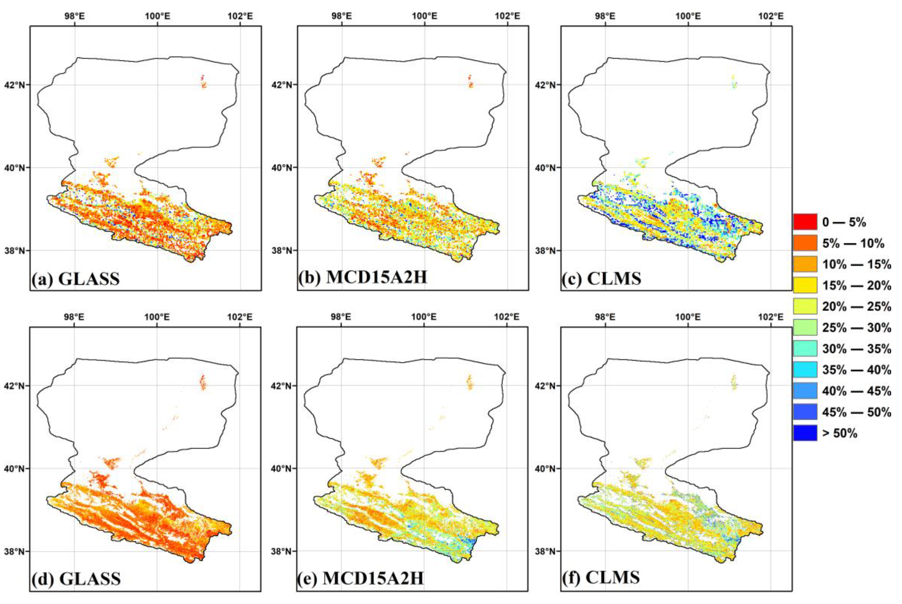
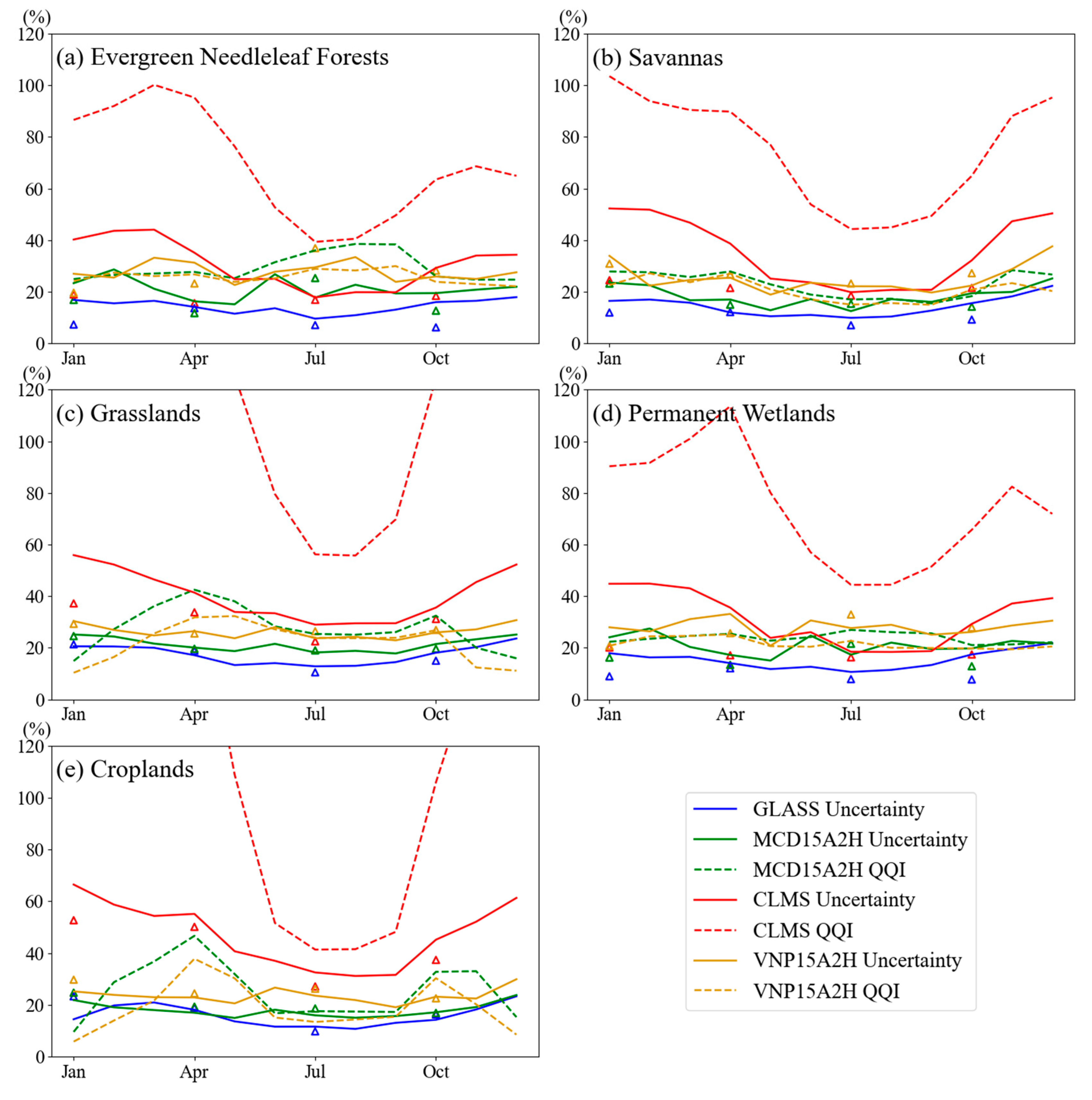
4.3. Relative Uncertainties

Overall, the pattern of relative uncertainties in summer still follows the order of GLASS < MCD15A2H < VNP15A2H/CLMS, with the main differences between methods manifesting in the magnitude of relative uncertainties for CLMS and VNP15A2H (Table 1 and Table 2). The results of the TC analysis using grid cells have a weak correlation with the spatial distribution of the LAI values, suggesting that relative uncertainties may reflect inherent differences between the products. Except for CLMS, which still exhibits greater relative uncertainties in croplands, all product relative uncertainty maps significantly differ from their absolute uncertainties (Figure 9, Figure A5 and Figure A6). Higher relative uncertainties are observed at the boundaries of land cover types or ecological transition zones, such as between grasslands and barren areas. When TC analysis is performed using pixel-scale temporal series, relative uncertainty maps yield similar conclusions but more clearly reflect the significant relative uncertainties of CLMS and MCD15A2H in croplands during summer, indicating the slightly poorer performance of these products in this region. VNP15A2H exhibits more significant relative noise than does the first method, partly due to its lower LAI values (Table 2) and its poorer performance in estimating LAI changes in the growing season (Figure 7). GLASS generally has low relative uncertainties (<10%) during summer but shows that areas with low absolute uncertainties have slightly greater relative uncertainties, possibly due to the calculation method of relative uncertainties and low LAI values.
Compared to the absolute uncertainties, the seasonal changes in the relative uncertainties are very minimal (Figure 10). The relative sizes of the uncertainties among products in different seasons follow the same pattern as the absolute uncertainties. For most land cover types and products, the relative uncertainties from the pixel-scale TC analysis are similar or slightly lower than those from the grid cell analysis and exhibit the same patterns: GLASS consistently has excellent stability (<25%); MCD15A2H exhibits relative uncertainties near those of GLASS in grasslands, croplands, and savannas but has significantly higher values in needleleaf forests and permanent wetlands during summer, though overall less than 30%. VNP15A2H and MCD15A2H have similar patterns in relation to land cover type and season, but the former has higher noise levels. Like absolute uncertainties, except in needleleaf forests and permanent wetlands during summer, the relative uncertainties of CLMS are slightly greater than those of other products across all biomes (approximately 25–70%), with a pattern of slightly greater values in winter than in summer, which is related to the high absolute uncertainties and underestimation of the LAI values of CLMS in winter. Similar to the summer relative uncertainty maps, in other seasons, the relative uncertainties of the products do not have significant differences related to land cover types.
Figure 10 also compares the TCEM relative uncertainties with the relative QQIs. The CLMS relative QQI has the same seasonal changes as the TCEM relative uncertainties, which is particularly evident in grasslands and croplands due to the nearly zero LAI values in winter in these biomes. MCD15A2H and VNP15A2H exhibit similar seasonal variations in relative QQIs in grasslands and croplands but with smaller amplitudes and virtually no seasonal differences in other land cover types. Consistent with the TCEM estimates, the relative QQI of CLMS is greater than that of MCD15A2H. The relative QQIs of the VNP15A2H and MCD15A2H and the relative uncertainties of the TCEM are fairly close across various land cover types. However, the relative QQI of CLMS is significantly greater than its TCEM uncertainties, indicating potential overestimation. A winter bias is observed in these products, with higher uncertainties in snow-covered conditions. This is likely due to the very low LAI values in winter, which magnify relative uncertainties. Specifically, the CLMS retrievals exhibit the most significant winter bias, possibly due to the high sensitivity of CLMS to the presence of snow, which can further amplify the uncertainty in these conditions.
Only GLASS meets GCOS’s relative precision requirement (20%) across all seasons, while the other three products only partially meet this requirement in needleleaf forests, savannas, and grasslands during July and August. The precision of VNP15A2H and MCD15A2H is close to 20% across all seasons. However, it should be noted that these conclusions apply only to averages across various land covers. Table 3 provides the specific percentage of pixels that meet the CEOS standards for each product. The trend of eligible pixels aligns well with the trends seen in the uncertainty maps and relative uncertainty maps. Overall, all products have a decrease in the percentage of eligible pixels during the growing season. More than 90% of GLASS, MCD15A2H, and VNP15A2H meet the absolute uncertainty requirement, and CLMS also achieves high precision, but its percentage meeting the requirements decreases to its lowest value in July (74.5%). This change in eligible pixel percentages contrasts with findings by Fang et al. [27], which can be attributed to the cold and arid climate of the Heihe River Basin and the types of vegetation present. Due to lower LAI values, the relative errors inherent in various remote sensing products are larger and seldom provide meaningful LAI information or are dominated by noise. Analyzing product performance in areas with scant valid information may lead to representational issues. In terms of relative uncertainty, the seasonal variation in the percentage of eligible pixels contrasts with the absolute uncertainties, being greater in summer than in winter. Significant performance gaps appear between products, with GLASS reaching up to 84.9% and CLMS meeting only 30.6% of the precision requirements. Similar results are obtained when analyzing time series data, which generally yields a slightly greater assessment of product accuracy.

5. Discussion

5.1. Performance of the Triple Collocation Method

This study primarily focuses on the theoretical uncertainties of the products, which can be linked to uncertainties in the input data and model simplifications. Physical uncertainties resemble systematic errors, whereas the TCEM quantifies theoretical uncertainties approximating random errors, which serve as a good indicator of the existing uncertainties between different products [9]. Although several products provide systematic QQIs, differences in error propagation schemes and definitions of uncertainty might lead to inconsistent uncertainty estimates between products. While QQIs cannot be used directly for product uncertainty evaluation, their time series can be utilized to determine the temporal evolution of product quality, providing a reference for independent validation. Good consistency with QQIs (Figure 7, Figure 8 and Figure 10) indicates that, as an independent verification method, the TC method offers a unified uncertainty index and is highly flexible, allowing for the quick estimation of uncertainty for triple LAI products.
As mentioned in Section 4, the two application methods of the TCEM yielded highly consistent results. In most cases, seasonal uncertainty is slightly lower than the results obtained through a grid-based approach. However, MCD15A2H and VNP15A2H show the opposite trend in certain biomes, particularly for relative uncertainty. It is difficult to determine which method provides more accurate conclusions, as the temporal “noise” mentioned earlier could either represent actual product errors or serve as evidence of the LUT algorithm’s sensitivity to LAI changes. One approach incurs accuracy loss in space, while the other incurs accuracy loss in time, and better uncertainty maps could potentially be achieved through data fusion.
The two implementations of the TCEM each offer distinct advantages and are designed to capture different aspects of product uncertainty. The first approach, which analyzes uncertainty within grid cells (0.025° resolution), focuses on the spatial distribution of the LAI within a defined area. This method aggregates uncertainty across space, reflecting how well the products capture the spatial patterns of the LAI. In contrast, the second approach focuses on uncertainty analysis at the pixel scale (0.005° resolution), which provides a finer-grained evaluation of temporal changes in the LAI for individual pixels. By applying a linear model fit to the time series data for each pixel, this approach is more capable of capturing subtle seasonal and temporal shifts that may be lost in the spatial aggregation of the first method.
Due to differences in input reflectance and retrieval algorithms, significant variations exist between different LAI products. For example, CLMS performs poorly in TC analysis, and previous studies have indicated that CLMS tends to overestimate LAIs. Systematic overestimation is primarily attributed to (1) the use of the blue band, which is sensitive to atmospheric effects, and (2) the use of the top-of-aerosol reflectance after partial atmospheric correction as the input data [57,58]. It is also worth noting that the CLMS product update in July 2020 may have introduced additional uncertainties, particularly for biomes with a smaller representation in the Heihe River Basin, such as savannas and needleleaf forests. These biomes exhibited noticeable discontinuities in their LAI observations (Figure 3). In contrast, GLASS, which also uses a neural network (NN) algorithm, shows the smallest uncertainties among all products. GLASS benefits from the fact that the algorithm utilizes MODIS reflectance data from an entire year to estimate the yearly LAI profile, thereby better capturing seasonality and reducing uncertainty [57]. Additionally, Jin et al. highlighted that the MODIS reflectance input is reprocessed to eliminate adverse weather effects before the General Regression Neural Network (GRNN) algorithm is applied to estimate the LAI, which further enhances the product’s accuracy and reduces uncertainty [21]. The overlap in uncertainty between MCD15A2H and VNP15A2H can be attributed to their reliance on similar surface reflectance models and retrieval algorithms. Both products estimate vegetation indices using comparable models, which means that they may exhibit similar error patterns when estimating vegetation changes under the same meteorological and surface conditions. Furthermore, both products employ similar inversion and correction algorithms, exposing them to common sources of error such as cloud interference, image stitching errors, and atmospheric correction issues.
The limited availability of training data in cropland areas might explain the greater uncertainties in those regions, especially during the growing season. Fang et al. noted that high uncertainties could be related to changes in input reflectance, especially during peak growing seasons [55]. High uncertainties in cropland areas are associated with the incomplete uniformity of crop fields, where bare soil, laid roads, and ditches may exist within fields.

5.2. Limitations and Future Prospects

The traditional application of the TCEM targeting in situ measurements, satellite observations, and model fields faces representativeness issues due to often differing scales involved with instruments and models. Using triplets of satellite products, the challenge arises in fulfilling the noncorrelation requirement of errors [59], which can be compromised by the use of similar satellite input data and preprocessing schemes, such as atmospheric corrections. Specifically, in this study’s products, MCD15A2H and VNP15A2H use the same LUT algorithm, and GLASS V6 utilizes MODIS and CLMS data to build time series LAI samples during its deep learning model training phase. When analyzing uncertainties across different land cover types, we found that the uncertainties for specific products derived from different combinations were quite similar. The largest absolute uncertainties were in summer, reaching up to ±0.1, while the uncertainties were approximately ±0.05 at other times. Relative uncertainties were also within 10%. However, uncertainty maps and the percentage of pixels meeting relative accuracy standards show nonnegligible differences at finer spatial scales when different combinations are used in TC analysis. However, according to Yilmaz and Crow, significant nonzero error cross-correlation still exists in dataset combinations typically considered to have zero error cross-correlation, such as between active and passive satellite data [60]. To our knowledge, no reliable method has yet been proposed to estimate error cross-correlation across broader scales. Fang et al. suggested that incorporating in situ observations or high-resolution LAI estimates in the TCEM could reveal these residuals and yield more robust error estimates [27].
Whether analyzing within grid cells or using pixel-scale seasonal time series, there are representativeness issues. The former, due to lower-resolution spatial partitioning, is easily influenced by other land cover types within the cell when conducting uncertainty analysis specific to land cover types. The needleleaf forests, savannas, and permanent wetlands in this study are typically found in mixed grid cells. Expanding the study area to cover more continuous, homogeneous land cover can mitigate this impact. The latter method addresses the representativeness issue spatially to some extent but also introduces new challenges: (1) reduced temporal resolution of uncertainties, which is undesirable in dynamic analysis; and (2) reduced number of samples in the dataset for TCEM analysis after segmenting the time series seasonally, facing statistical challenges. By expanding the study period and increasing sample sizes while allowing shorter temporal segments, this can be accommodated if products provide long-term LAI data. Additionally, optimizing the slicing of the time series into a sliding window could dynamically obtain uncertainties for each window, constructing a more detailed temporal change relationship.
This method only provides valid estimates in regions with effective triplets and sufficiently high product correlation. It should be noted that the four product combinations selected in this study meet these criteria in most areas of the Heihe River Basin during summer, but only approximately 12.5% of the pixels meet these criteria in winter, and the representativeness of the results needs further verification. Apart from these requirements, the TC method may also fail under certain conditions, such as when the variance of internal samples in observational data is small, which could lead to division by zero errors and numerical instability when calculating scaling coefficients. Recently, Kim et al.’s approach of using machine learning methods to fill in soil moisture uncertainty maps in regions where the triple collocation method fails could be highly instructive [61]. It is important to emphasize that the TC method is limited to calculating the theoretical uncertainty of LAI products and assessing their relative performance. However, practical in situ validation remains essential, particularly in regions and during periods where theoretical uncertainty of the products is high, such as cropland areas and high-altitude regions (e.g., rugged mountainous areas). To address these gaps, we are currently advancing direct upscaling validation efforts in the Heihe River Basin.
While our study provides product uncertainty estimates in the form of RMSE, we have also calculated the standard deviations of these uncertainty estimates. This represents an advancement over previous studies on the LAI [27], wind speed [43], and soil moisture [47], which primarily focused on RMSE or error variances without emphasizing the dispersion of uncertainty estimates. Although we have included the standard deviation of uncertainty, further investigation is required to fully understand its significance and its reference value in assessing LAI product uncertainty. We plan to explore this aspect in greater depth in future research. Moreover, incorporating recent advances in LAI retrieval methods may further enhance the accuracy and robustness of our uncertainty assessments, and we are committed to integrating these advanced methods in our future work.

6. Conclusions

This study conducted an in-depth intercomparison and quality assessment of four LAI products—GLASS, MCD15A2H, VNP15A2H, and CLMS—closely aligned in time and space for the Heihe River Basin using the triple collocation error model to explore the inherent temporal and spatial uncertainties of these products. Rigorous analyses across different land cover types and seasons revealed subtle performance nuances of these satellite-derived LAI products, highlighting the critical role of sensors and retrieval algorithms in their accuracy and reliability.
The key findings indicate that these four LAI products’ theoretical uncertainties generally meet the GCOS accuracy requirement of ±0.5 in most biome types during the growing season, with GLASS consistently showing the lowest uncertainties and CLMS displaying the highest, especially in cropland areas. Fang et al. also noted that for grasslands, the RMSE of LAI products can be controlled within 0.5. However, many previous studies have demonstrated that, based on direct validation against field measurements or reference maps, current LAI products usually fail to meet the accuracy requirements of GCOS. This contradiction may arise from the specific characteristics of the study area and also reveals the limitations of the TC method itself.
Additionally, comparative analyses revealed that relative uncertainties vary across different biome types, with more pronounced differences in areas with complex vegetation cover, such as croplands, indicating greater sensitivity to algorithm differences in these environments. Regarding product performance, GLASS generally performs the best, followed by MCD15A2H and VNP15A2H, which are highly sensitive to short-term changes in the LAI, exhibiting more noticeable value variations. Although CLMS has slightly lower accuracy, its performance can surpass MCD15A2H and VNP15A2H during the growing season, especially in needleleaf forest and permanent wetland areas.
While the TCEM provides a unified metric for measuring the relative performance between products without relying on ground-truth data, it also has limitations, particularly regarding the assumption of noncorrelation among errors between products. The findings emphasize the need for ongoing improvements in satellite data processing techniques and the development of more robust models capable of accounting for complex interactions between land cover types and satellite observation systems. Given the independence assumption of the products, further improvements to the TC algorithm are necessary. For a more comprehensive evaluation of uncertainty, it is also crucial to incorporate field measurements and high-resolution reference maps.

Author Contributions

Conceptualization, L.G.; methodology, P.Z.; software, P.Z.; formal analysis, P.Z.; investigation, P.Z.; data curation, H.W.; writing—original draft, P.Z.; writing—review and editing, L.G., J.L., and H.W.; funding acquisition, L.G. and H.W. All authors have read and agreed to the published version of the manuscript.

Funding

This work was supported by the National Natural Science Foundation of China under Grant No. 42171390 and 42371405; and Key Research Program of Gansu Province under Grant No. 23ZDKA0004.

Data Availability Statement

The LAI remote sensing products evaluated here are freely available online: MCD15A2H form https://lpdaac.usgs.gov/products/mcd15a2hv061/; VNP15A2H from https://lpdaac.usgs.gov/products/vnp15a2hv002/; CLMS from https://land.copernicus.eu/en/products/vegetation/leaf-area-index-300m-v1.0; and GLASS from https://glass.bnu.edu.cn/introduction/LAI.html. The land cover type dataset and the DEM dataset are both available online: MCD12Q1 at https://lpdaac.usgs.gov/products/mcd12q1v061/ and ASTER GDEM at https://gdemdl.aster.jspacesystems.or.jp/index.html.

Conflicts of Interest

The authors declare no conflicts of interest.

Appendix A

LAI, difference, correlation, and uncertainty maps for all products and triplet combinations.
Figure A1. Maps of LAIs from GLASS, MCD15A2H, CLMS, and VNP15A2H (ad), their differences (ej) and their correlations (kp). Temporal resolution: (aj) July monthly composite for the year 2021; (kp) July monthly composite for years 2018–2021. Spatial resolution (pixel size): (aj) 0.005° × 0.005°; (kp) 0.025° × 0.025°.
Remotesensing 17 01233 g0a1
Figure A2. Uncertainty maps of the four products in the Heihe River Basin in July obtained through TC analysis within grid cells (0.025° × 0.025°). Each row presents the results for different triplet combinations.
Remotesensing 17 01233 g0a2
Figure A3. Uncertainty maps of the four products in the Heihe River Basin in summer derived from TC analysis at the pixel scale using seasonal time series segmentation (0.005° × 0.005°). Each row presents the results for different triplet combinations.
Remotesensing 17 01233 g0a3
Figure A4. Variation in the standard deviation of the uncertainty data. The solid lines represent the standard deviation of the monthly uncertainties calculated by the first method; the standard deviation of the seasonal uncertainties estimated by the second method are represented by triangles corresponding to April, July, October, and January.
Remotesensing 17 01233 g0a4
Figure A5. Relative uncertainty maps of the four products in the Heihe River Basin in July obtained through TC analysis within grid cells (0.025° × 0.025°). Each row presents the results for different triplet combinations.
Remotesensing 17 01233 g0a5
Figure A6. Relative uncertainty maps of the four products in the Heihe River Basin in summer derived from TC analysis at the pixel scale using seasonal time series segmentation (0.005° × 0.005°). Each row presents the results for different triplet combinations.
Remotesensing 17 01233 g0a6

References

  1. Chen, J.M.; Black, T.A. Defining Leaf Area Index for Non-Flat Leaves. Plant Cell Environ. 1992, 15, 421–429. [Google Scholar] [CrossRef]
  2. Al-Kaisi, M.; Brun, L.J.; Enz, J.W. Transpiration and Evapotranspiration from Maize as Related to Leaf Area Index. Agric. For. Meteorol. 1989, 48, 111–116. [Google Scholar] [CrossRef]
  3. Alton, P.B. Decadal Trends in Photosynthetic Capacity and Leaf Area Index Inferred from Satellite Remote Sensing for Global Vegetation Types. Agric. For. Meteorol. 2018, 250–251, 361–375. [Google Scholar] [CrossRef]
  4. Jarlan, L.; Balsamo, G.; Lafont, S.; Beljaars, A.; Calvet, J.C.; Mougin, E. Analysis of Leaf Area Index in the ECMWF Land Surface Model and Impact on Latent Heat and Carbon Fluxes: Application to West Africa. J. Geophys. Res. Atmos. 2008, 113, D24117. [Google Scholar] [CrossRef]
  5. Belward, A.; Bourassa, M.; Dowell, M.; Briggs, S.; Dolman, H.A.J.; Holmlund, K.; Husband, R.; Quegan, S.; Simmons, A.; Sloyan, B.; et al. The Global Observing System for Climate: Implementation Needs; World Meteorological Organization: Geneva, Switzerland, 2016. [Google Scholar]
  6. Hirofumi, H.; Wang, W.; Milesi, C.; White, M.A.; Ganguly, S.; Gamo, M.; Hirata, R.; Myneni, R.B.; Nemani, R.R. Exploring Simple Algorithms for Estimating Gross Primary Production in Forested Areas from Satellite Data. Remote Sens. 2012, 4, 303–326. [Google Scholar] [CrossRef]
  7. Ray, L.; Zhang, Y.Q.; Rajaud, A.; Cleugh, H.; Tu, K. A Simple Surface Conductance Model to Estimate Regional Evaporation Using MODIS Leaf Area Index and the Penman-Monteith Equation. Water Resour. Res. 2008, 44, W10419. [Google Scholar] [CrossRef]
  8. Donohue, R.J.; Roderick, M.L.; McVicar, T.R. On the Importance of Including Vegetation Dynamics in Budyko’s Hydrological Model. Hydrol. Earth Syst. Sci. 2007, 11, 983–995. [Google Scholar] [CrossRef]
  9. Fang, H.; Baret, F.; Plummer, S.; Schaepman-Strub, G. An Overview of Global Leaf Area Index (LAI): Methods, Products, Validation, and Applications. Rev. Geophys. 2019, 57, 739–799. [Google Scholar] [CrossRef]
  10. Fernandes, R.; Plummer, S.; Nightingale, J.; Baret, F.; Camacho, F.; Fang, H.; Garrigues, S.; Gobron, N.; Lang, M.; Lacaze, R.; et al. Global leaf area index product validation good practices, in Best practice for satellite-derived land product validation, 2.0. In Land Product Validation Subgroup; Fernandes, R., Plummer, S., Nightingale, J., Eds.; Committee on Earth Observation Satellites Working Group on Calibration and Validation: Greenbelt, MD, USA, 2014. [Google Scholar] [CrossRef]
  11. Li, X.; Ma, M.; Wang, J.; Liu, Q.; Che, T.; Hu, Z.; Xiao, Q.; Liu, Q. Simultaneous Remote Sensing and Ground-based Experiment in the Heihe River Basin: Scientific Objectives and Experiment Design. Adv. Earth Sci. 2008, 23, 897–914. [Google Scholar]
  12. Li, X.; Li, X.; Li, Z. Watershed Allied Telemetry Experimental Research (WATER) Datasets are Available for Open Access. Remote Sens. Technol. Appl. 2010, 25, 761–765. [Google Scholar] [CrossRef]
  13. Li, X.; Wang, S.G.; Ge, Y.; Jin, R.; Liu, S.M.; Ma, M.G.; Shi, W.Z.; Li, R.X.; Liu, Q.H. Development and Experimental Verification of Key Techniques to Validate Remote Sensing Products. ISPRS Int. Arch. Photogramm. Remote Sens. Spat. Inf. Sci. 2013, XL-2/W1, 25–30. [Google Scholar] [CrossRef]
  14. Zhang, Y.; Qu, Y.; Wang, J.; Liang, S.; Liu, Y. Estimating Leaf Area Index from MODIS and Surface Meteorological Data Using a Dynamic Bayesian Network. Remote Sens. Environ. 2012, 127, 30–43. [Google Scholar] [CrossRef]
  15. Chen, Y.P.; Wei, W.; Patterson, A.E.; Tong, L. Spatial Scale Conversion Approach for Moderate-Resolution Imaging Spectroradiometer Leaf Area Index Product Validation. J. Appl. Remote Sens. 2013, 7, 073463. [Google Scholar] [CrossRef]
  16. Qu, Y.; Han, W.; Ma, M. Retrieval of a Temporal High-Resolution Leaf Area Index (LAI) by Combining MODIS LAI and ASTER Reflectance Data. Remote Sens. 2015, 7, 195–210. [Google Scholar] [CrossRef]
  17. Shi, Y.; Wang, J.; Qin, J.; Qu, Y. An Upscaling Algorithm to Obtain the Representative Ground Truth of LAI Time Series in Heterogeneous Land Surface. Remote Sens. 2015, 7, 12887–12908. [Google Scholar] [CrossRef]
  18. Buermann, W.; Wang, Y.; Dong, J.; Zhou, L.; Zeng, X.; Dickinson, R.E.; Potter, C.S.; Myneni, R.B. Analysis of a Multiyear Global Vegetation Leaf Area Index Data Set. J. Geophys. Res. Atmos. 2002, 107, 14–16. [Google Scholar] [CrossRef]
  19. Kang, H.-S.; Xue, Y.; Collatz, G.J. Impact Assessment of Satellite-Derived Leaf Area Index Datasets Using a General Circulation Model. J. Clim. 2007, 20, 993–1015. [Google Scholar] [CrossRef]
  20. Camacho, F.; Cernicharo, J.; Lacaze, R.; Baret, F.; Weiss, M. GEOV1: LAI, FAPAR Essential Climate Variables and FCOVER Global Time Series Capitalizing over Existing Products. Part 2: Validation and Intercomparison with Reference Products. Remote Sens. Environ. 2013, 137, 310–329. [Google Scholar] [CrossRef]
  21. Jin, H.; Li, A.; Bian, J.; Nan, X.; Zhao, W.; Zhang, Z.; Yin, G. Intercomparison and Validation of MODIS and GLASS Leaf Area Index (LAI) Products over Mountain Areas: A Case Study in Southwestern China. Int. J. Appl. Earth Obs. Geoinf. 2017, 55, 52–67. [Google Scholar] [CrossRef]
  22. D’Odorico, P.; Gonsamo, A.; Pinty, B.; Gobron, N.; Coops, N.; Mendez, E.; Schaepman, M.E. Intercomparison of Fraction of Absorbed Photosynthetically Active Radiation Products Derived from Satellite Data over Europe. Remote Sens. Environ. 2014, 142, 141–154. [Google Scholar] [CrossRef]
  23. Xu, B.; Li, J.; Park, T.; Liu, Q.; Zeng, Y.; Yin, G.; Zhao, J.; Fan, W.; Yang, L.; Knyazikhin, Y.; et al. An Integrated Method for Validating Long-Term Leaf Area Index Products Using Global Networks of Site-Based Measurements. Remote Sens. Environ. 2018, 209, 134–151. [Google Scholar] [CrossRef]
  24. Croft, H.; Chen, J.M.; Zhang, Y. Temporal Disparity in Leaf Chlorophyll Content and Leaf Area Index across a Growing Season in a Temperate Deciduous Forest. Int. J. Appl. Earth Obs. Geoinf. 2014, 33, 312–320. [Google Scholar] [CrossRef]
  25. Zhu, Z.; Bi, J.; Pan, Y.; Ganguly, S.; Anav, A.; Xu, L.; Samanta, A.; Piao, S.; Nemani, R.R.; Myneni, R.B. Global Data Sets of Vegetation Leaf Area Index (LAI)3g and Fraction of Photosynthetically Active Radiation (FPAR)3g Derived from Global Inventory Modeling and Mapping Studies (GIMMS) Normalized Difference Vegetation Index (NDVI3g) for the Period 1981 to 2011. Remote Sens. 2013, 5, 927–948. [Google Scholar] [CrossRef]
  26. Anav, A.; Murray-Tortarolo, G.; Friedlingstein, P.; Sitch, S.; Piao, S.; Zhu, Z. Evaluation of Land Surface Models in Reproducing Satellite Derived Leaf Area Index over the High-Latitude Northern Hemisphere. Part II: Earth System Models. Remote Sens. 2013, 5, 3637–3661. [Google Scholar] [CrossRef]
  27. Fang, H.; Wei, S.; Jiang, C.; Scipal, K. Theoretical Uncertainty Analysis of Global MODIS, CYCLOPES, and GLOBCARBON LAI Products Using a Triple Collocation Method. Remote Sens. Environ. 2012, 124, 610–621. [Google Scholar] [CrossRef]
  28. García-Haro, F.J.; Campos-Taberner, M.; Muñoz-Marí, J.; Laparra, V.; Camacho, F.; Sánchez-Zapero, J.; Camps-Valls, G. Derivation of Global Vegetation Biophysical Parameters from EUMETSAT Polar System. ISPRS J. Photogramm. Remote Sens. 2018, 139, 57–74. [Google Scholar] [CrossRef]
  29. Xiao, Z.; Liang, S.; Wang, J.; Chen, P.; Yin, X.; Zhang, L.; Song, J. Use of General Regression Neural Networks for Generating the GLASS Leaf Area Index Product from Time-Series MODIS Surface Reflectance. IEEE Trans. Geosci. Remote Sens. 2014, 52, 209–223. [Google Scholar] [CrossRef]
  30. Frederic, B.; Hagolle, O.; Geiger, B.; Bicheron, P.; Miras, B.; Huc, M.; Berthelot, B.; Niño, F.; Weiss, M.; Samain, O.; et al. LAI, fAPAR and fCover CYCLOPES Global Products Derived from VEGETATION: Part 1: Principles of the Algorithm. Remote Sens. Environ. 2007, 110, 275–286. [Google Scholar] [CrossRef]
  31. Knyazikhin, Y.; Martonchik, J.V.; Diner, D.J.; Myneni, R.B.; Verstraete, M.; Pinty, B.; Gobron, N. Estimation of Vegetation Canopy Leaf Area Index and Fraction of Absorbed Photosynthetically Active Radiation from Atmosphere-Corrected MISR Data. J. Geophys. Res. Atmos. 1998, 103, 32239–32256. [Google Scholar] [CrossRef]
  32. Yan, K.; Park, T.; Chen, C.; Xu, B.; Song, W.; Yang, B.; Zeng, Y.; Liu, Z.; Yan, G. Generating Global Products of LAI and FPAR From SNPP-VIIRS Data: Theoretical Background and Implementation. IEEE Trans. Geosci. Remote Sens. 2018, 56, 2119–2137. [Google Scholar] [CrossRef]
  33. Pinty, B.; Andredakis, I.; Clerici, M.; Kaminski, T.; Taberner, M.; Verstraete, M.M.; Gobron, N.; Plummer, S.; Widlowski, J.-L. Exploiting the MODIS Albedos with the Two-Stream Inversion Package (JRC-TIP): 1. Effective Leaf Area Index, Vegetation, and Soil Properties. J. Geophys. Res. Atmos. 2011, 116, 1–20. [Google Scholar] [CrossRef]
  34. McColl, K.A.; Vogelzang, J.; Konings, A.G.; Entekhabi, D.; Piles, M.; Stoffelen, A. Extended Triple Collocation: Estimating Errors and Correlation Coefficients with Respect to an Unknown Target. Geophys. Res. Lett. 2014, 41, 6229–6236. [Google Scholar] [CrossRef]
  35. Ganguly, S.; Samanta, A.; Shabanov, N.; Cristina, M.; Nemani, R.; Knyazikhin, Y.; Myneni, R. Generating Vegetation Leaf Area Index Earth System Data Record from Multiple Sensors. Part 1: Theory. Remote Sens. Environ. 2008, 112, 4333–4343. [Google Scholar] [CrossRef]
  36. Yan, K.; Park, T.; Yan, G.; Liu, Z.; Yang, B.; Chen, C.; Nemani, R.R.; Knyazikhin, Y.; Myneni, R.B. Evaluation of MODIS LAI/FPAR Product Collection 6. Part 2: Validation and Intercomparison. Remote Sens. 2016, 8, 460. [Google Scholar] [CrossRef]
  37. Xu, B.; Park, T.; Yan, K.; Chen, C.; Zeng, Y.; Song, W.; Yin, G.; Li, J.; Liu, Q.; Knyazikhin, Y.; et al. Analysis of Global LAI/FPAR Products from VIIRS and MODIS Sensors for Spatio-Temporal Consistency and Uncertainty from 2012–2016. Forests 2018, 9, 73. [Google Scholar] [CrossRef]
  38. Zhang, X.; Liu, L.; Liu, Y.; Jayavelu, S.; Wang, J.; Moon, M.; Henebry, G.M.; Friedl, M.A.; Schaaf, C.B. Generation and Evaluation of the VIIRS Land Surface Phenology Product. Remote Sens. Environ. 2018, 216, 212–229. [Google Scholar] [CrossRef]
  39. Justice, C.O.; Román, M.O.; Csiszar, I.; Vermote, E.F.; Wolfe, R.E.; Hook, S.J.; Friedl, M.; Wang, Z.; Schaaf, C.B.; Miura, T.; et al. Land and Cryosphere Products from Suomi NPP VIIRS: Overview and Status. J. Geophys. Res. Atmos. 2013, 118, 9753–9765. [Google Scholar] [CrossRef]
  40. Fuster, B.; Sánchez-Zapero, J.; Camacho, F.; García-Santos, V.; Verger, A.; Lacaze, R.; Weiss, M.; Baret, F.; Smets, B. Quality Assessment of CLMS LAI, fAPAR and fCOVER Collection 300 m Products of Copernicus Global Land Service. Remote Sens. 2020, 12, 1017. [Google Scholar] [CrossRef]
  41. Ma, H.; Liang, S. Development of the GLASS 250-m Leaf Area Index Product (Version 6) from MODIS Data Using the Bidirectional LSTM Deep Learning Model. Remote Sens. Environ. 2022, 273, 112985. [Google Scholar] [CrossRef]
  42. Stoffelen, A. Toward the True Near-Surface Wind Speed: Error Modeling and Calibration Using Triple Collocation. J. Geophys. Res. Ocean. 1998, 103, 7755–7766. [Google Scholar] [CrossRef]
  43. Portabella, M.; Stoffelen, A. On Scatterometer Ocean Stress. J. Atmos. Ocean. Technol. 2009, 26, 368–382. [Google Scholar] [CrossRef]
  44. Vogelzang, J.; Stoffelen, A.; Verhoef, A.; Figa-Saldaña, J. On the Quality of High-Resolution Scatterometer Winds. J. Geophys. Res. Ocean. 2011, 116, 5565. [Google Scholar] [CrossRef]
  45. Caires, S.; Sterl, A. Validation of Ocean Wind and Wave Data Using Triple Collocation. J. Geophys. Res. Ocean. 2003, 108, 3098. [Google Scholar] [CrossRef]
  46. Janssen, P.A.E.M.; Abdalla, S.; Hersbach, H.; Bidlot, J.-R. Error Estimation of Buoy, Satellite, and Model Wave Height Data. J. Atmos. Ocean. Technol. 2007, 24, 1665–1677. [Google Scholar] [CrossRef]
  47. Scipal, K.; Holmes, T.; de Jeu, R.; Naeimi, V.; Wagner, W. A Possible Solution for the Problem of Estimating the Error Structure of Global Soil Moisture Data Sets. Geophys. Res. Lett. 2008, 35, L24403. [Google Scholar] [CrossRef]
  48. Kim, H.; Wigneron, J.-P.; Kumar, S.; Dong, J.; Wagner, W.; Cosh, M.H.; Bosch, D.D.; Collins, C.H.; Starks, P.J.; Seyfried, M.; et al. Global Scale Error Assessments of Soil Moisture Estimates from Microwave-Based Active and Passive Satellites and Land Surface Models over Forest and Mixed Irrigated/Dryland Agriculture Regions. Remote Sens. Environ. 2020, 251, 112052. [Google Scholar] [CrossRef]
  49. Chen, F.; Crow, W.T.; Bindlish, R.; Colliander, A.; Burgin, M.S.; Asanuma, J.; Aida, K. Global-Scale Evaluation of SMAP, SMOS and ASCAT Soil Moisture Products Using Triple Collocation. Remote Sens. Environ. 2018, 214, 1–13. [Google Scholar] [CrossRef] [PubMed]
  50. Loew, A.; Schlenz, F. A Dynamic Approach for Evaluating Coarse Scale Satellite Soil Moisture Products. Hydrol. Earth Syst. Sci. 2011, 15, 75–90. [Google Scholar] [CrossRef]
  51. Gruber, A.; Su, C.-H.; Zwieback, S.; Crow, W.; Dorigo, W.; Wagner, W. Recent Advances in (Soil Moisture) Triple Collocation Analysis. Int. J. Appl. Earth Obs. Geoinf. 2016, 45, 200–211. [Google Scholar] [CrossRef]
  52. Su, C.-H.; Ryu, D.; Crow, W.T.; Western, A.W. Beyond Triple Collocation: Applications to Soil Moisture Monitoring. J. Geophys. Res. Atmos. 2014, 119, 6419–6439. [Google Scholar] [CrossRef]
  53. Yilmaz, M.T.; Crow, W.T. The Optimality of Potential Rescaling Approaches in Land Data Assimilation. J. Hydrol. 2013, 14, 650–660. [Google Scholar] [CrossRef]
  54. Gessner, U.; Niklaus, M.; Kuenzer, C.; Dech, S. Intercomparison of Leaf Area Index Products for a Gradient of Sub-Humid to Arid Environments in West Africa. Remote Sens. 2013, 5, 1235–1257. [Google Scholar] [CrossRef]
  55. World Meteorological Organization (WMO); United Nations Environment Programme (UNEP); International Science Council (ISC); Scientific and Cultural Organization (IOC-UNESCO). Intergovernmental Oceanographic Commission of the United Nations Educational. The 2022 GCOS ECVs Requirements (GCOS 245). 2025. Available online: https://library.wmo.int/records/item/58111-the-2022-gcos-ecvs-requirements-gcos-245 (accessed on 18 January 2025).
  56. Tian, Y.; Dickinson, R.E.; Zhou, L.; Zeng, X.; Dai, Y.; Myneni, R.B.; Knyazikhin, Y.; Zhang, X.; Friedl, M.; Yu, H.; et al. Comparison of Seasonal and Spatial Variations of Leaf Area Index and Fraction of Absorbed Photosynthetically Active Radiation from Moderate Resolution Imaging Spectroradiometer (MODIS) and Common Land Model. J. Geophys. Res. Atmos. 2004, 109, D01103. [Google Scholar] [CrossRef]
  57. Fang, H.; Zhang, Y.; Wei, S.; Li, W.; Ye, Y.; Sun, T.; Liu, W. Validation of Global Moderate Resolution Leaf Area Index (LAI) Products over Croplands in Northeastern China. Remote Sens. Environ. 2019, 233, 111377. [Google Scholar] [CrossRef]
  58. Baret, F.; Weiss, M.; Verger, A.; Smets, B. ATBD for LAI, FAPAR and FCOVER from CLMS Products at 300M Resolution (GEOV3). IMAGINES\_RP2.1\_ATBD-LAI300M, 61. 2016. Available online: http://fp7-imagines.eu/pages/documents.php (accessed on 3 December 2023).
  59. He, Y.; Wang, C.; Hu, J.; Mao, H.; Duan, Z.; Qu, C.; Li, R.; Wang, M.; Song, X. Discovering Optimal Triplets for Assessing the Uncertainties of Satellite-Derived Evapotranspiration Products. Remote Sens. 2023, 15, 3215. [Google Scholar] [CrossRef]
  60. Yilmaz, M.T.; Crow, W.T. Evaluation of Assumptions in Soil Moisture Triple Collocation Analysis. J. Hydrometeorol. 2014, 15, 1293–1302. [Google Scholar] [CrossRef]
  61. Kim, H.; Crow, W.; Li, X.; Wagner, W.; Hahn, S.; Lakshmi, V. True Global Error Maps for SMAP, SMOS, and ASCAT Soil Moisture Data Based on Machine Learning and Triple Collocation Analysis. Remote Sens. Environ. 2023, 298, 113776. [Google Scholar] [CrossRef]
Figure 1. Aggregated land cover map based on MCD12Q1 (a) and the DEM (b) in the Heihe River Basin.
Remotesensing 17 01233 g001
Figure 2. Spatial distribution of the number of valid collocates in each grid cell in January (a) and July (b) from 2018 to 2021 (0.025° × 0.025°).
Remotesensing 17 01233 g002
Figure 3. The 10-day time series curves of the LAI for the four products across different land cover types in the Heihe River Basin from 2018 to 2022. The time series were obtained by compositing the maximum LAI values within each 10-day period for each original product, and the LAI values for each land cover type were calculated based on the MCD12Q1.
Remotesensing 17 01233 g003
Figure 4. Maps of LAIs from GLASS, MCD15A2H, and CLMS (ac), their differences (df), and their correlations (gi). Temporal resolution: (af) July monthly composite for 2021; (gi) July monthly composite for 2018–2021. Spatial resolution (pixel size): (af) 0.005° × 0.005°; (gi) 0.025° × 0.025°.
Remotesensing 17 01233 g004
Figure 5. Gaussian kernel density scatter plots of the LAI for grasslands and croplands.
Remotesensing 17 01233 g005
Figure 6. Uncertainty maps of GLASS, MCD15A2H, and CLMS in the Heihe River Basin in July obtained through TC analysis within grid cells (0.025° × 0.025°) (ac) and uncertainty maps in summer derived from TC analysis at the pixel scale using seasonal time series segmentation (0.005° × 0.005°) (df).
Remotesensing 17 01233 g006
Figure 7. Comparison of product uncertainty estimated by the TC method with QQIs from MCD15A2H, CLMS, and VNP15A2H. The solid lines represent the monthly uncertainties calculated by the first method; the dashed lines represent the QQIs of the products; the seasonal uncertainties estimated by the second method are represented by triangles corresponding to April, July, October, and January.
Remotesensing 17 01233 g007
Figure 8. Comparison of the QQIs and uncertainties calculated by the TCEM for the MCD15A2H (red), VNP15A2H (green), and CLMS (blue) products.
Remotesensing 17 01233 g008
Figure 9. Relative uncertainty maps of GLASS, MCD15A2H, and CLMS in the Heihe River Basin in July obtained through TC analysis within grid cells (0.025° × 0.025°) (ac) and relative uncertainty maps in summer derived from TC analysis at the pixel scale using seasonal time series segmentation (0.005° × 0.005°) (df).
Remotesensing 17 01233 g009
Figure 10. Comparison of product uncertainty estimated by the TC method with QQIs from MCD15A2H, CLMS, and VNP15A2H. The solid lines represent the monthly relative uncertainties calculated by the first method; the dashed lines represent the relative QQIs of the products; the seasonal relative uncertainties estimated by the second method are represented by triangles corresponding to April, July, October, and January.
Remotesensing 17 01233 g010
Table 1. Mean LAI and uncertainties estimated with the TCEM and QQI for the GLASS, MCD15A2H, CLMS, and VNP15A2H products. The LAI data included July monthly composites for four years (2018–2021). The last column shows the average value of all pixels. The last row shows the percentage of TCEM valid collocates in each biome.
ProductNeedleleaf ForestsSavannasGrasslandsPermanent WetlandsCroplandsOverall
Mean LAIGLASS3.171.511.132.682.181.27
MCD15A2H2.741.281.202.172.491.37
CLMS2.611.771.212.402.511.37
VNP15A2H2.311.201.032.002.261.20
Uncertainty TCEMGLASS0.240.160.130.240.220.14
MCD15A2H0.390.180.200.350.360.22
CLMS0.430.340.330.410.710.37
VNP15A2H0.570.290.240.480.470.27
Relative TCEM (%)GLASS9.559.8712.8110.6311.5712.64
MCD15A2H17.7212.4918.1717.3115.9417.89
CLMS17.8019.8128.9518.4532.5129.27
VNP15A2H29.4622.1123.6827.6323.5323.68
Uncertainty QQIGLASSN/AN/AN/AN/AN/AN/A
MCD15A2H1.010.230.230.630.440.26
CLMS0.990.750.510.930.920.56
VNP15A2H0.700.180.180.480.290.20
Relative QQI (%)GLASSN/AN/AN/AN/AN/AN/A
MCD15A2H36.0216.9825.3626.9317.5324.40
CLMS39.3244.2756.2044.4041.3554.43
VNP15A2H28.8814.9923.9122.6713.3822.51
valid collocates (%) 0.190.2185.970.5313.10100
Table 2. Mean LAI and uncertainties estimated with TC using time series slices and QQI for the GLASS, MCD15A2H, CLMS, and VNP15A2H products for different biome types. The LAI data included summer 10-day composites for four years (2018–2021). The last column shows the average value of all pixels.
ProductNeedleleaf ForestsSavannasGrasslandsPermanent WetlandsCroplandsOverall
Mean LAIGLASS2.90 1.350.952.381.771.06
MCD15A2H2.191.090.91.781.811.03
CLMS2.10 1.440.891.941.751.00
VNP15A2H1.850.960.771.50 1.620.88
Uncertainty TCEMGLASS0.20 0.10 0.10 0.190.170.11
MCD15A2H0.560.170.190.380.370.22
CLMS0.350.270.220.330.50 0.26
VNP15A2H0.660.230.230.480.450.27
Relative TCEM (%)GLASS7.067.0210.477.839.7310.34
MCD15A2H25.2915.30 18.9721.5518.5718.92
CLMS16.8318.4822.4716.2827.0923.10
VNP15A2H36.8823.1826.40 32.8826.2326.40
Table 3. The proportion of pixels reaching the GCOS accuracy requirements (absolute uncertainty: 0.5; relative uncertainty: 20%) for the GLASS, MCD15A2H, CLMS, and VNP15A2H data for each month.
Product123456789101112
Uncertainty
≤0.5
(%)
GLASS100.0100.0100.0100.0100.099.799.699.599.8100.0100.0100.0
MCD15A2H100.0100.0100.0100.099.996.091.193.498.599.799.999.9
CLMS99.9100.0100.0100.098.780.474.579.595.297.9100.0100.0
VNP15A2H100.0100.0100.0100.099.993.586.891.498.999.7100.0100.0
Relative
≤20%
(%)
GLASS55.851.354.370.384.980.483.282.578.970.055.933.6
MCD15A2H37.640.049.758.566.053.065.662.367.754.145.339.0
CLMS0.91.02.16.116.018.629.228.630.613.72.21.6
VNP15A2H23.724.729.130.142.931.144.343.246.834.931.023.1
Disclaimer/Publisher’s Note: The statements, opinions and data contained in all publications are solely those of the individual author(s) and contributor(s) and not of MDPI and/or the editor(s). MDPI and/or the editor(s) disclaim responsibility for any injury to people or property resulting from any ideas, methods, instructions or products referred to in the content.

