1. Introduction
Spaceborne LiDAR systems have become indispensable tools for Earth observation, providing critical data on forest structures, glacier dynamics, and natural hazards [
1,
2,
3]. They enable scientists to study environmental changes and processes with unprecedented detail, contributing significantly to our understanding of ecological systems. However, the current satellite LiDAR platforms, such as NASA’s GEDI [
4] and ICESat-2 [
5], face resolution constraints due to operational limitations like footprint size, photon acquisition rates, and onboard processing capacities. In contrast, airborne LiDAR systems like NASA’s G-LiHT [
6] produce high-resolution data but lack the global coverage and scalability required for comprehensive Earth observation. Bridging the resolution gap between satellite and airborne LiDAR systems could significantly advance remote sensing applications across multiple scientific domains.
A promising approach to address these challenges involves the use of Hyperheight Data Cubes (HHDCs), which provide a novel representation of LiDAR data that captures the three-dimensional structural information of landscapes [
7]. HHDCs are constructed by aggregating LiDAR returns into a three-dimensional tensor, with the dimensions representing spatial coordinates and height, effectively capturing the vertical distribution of features such as vegetation and terrain elevations. This rich representation not only facilitates advanced analyses of ecological structures but also works seamlessly with previous approaches by delivering traditional data products, such as Canopy Height Models (CHMs), Digital Terrain Models (DTMs), and Canopy Height Profiles (CHPs). By enabling the extraction of these conventional products within a unified framework, HHDCs ensure compatibility with existing methodologies while enhancing the potential for new insights. Moreover, HHDCs support advanced processing techniques, including footprint completion and super-resolution using Generative Adversarial Networks (GANs) [
8] and diffusion models [
9]. These methods can reconstruct missing or sparse data within HHDCs, improving the quality and resolution of the datasets. Additionally, by integrating HHDCs with other data modalities, such as hyperspectral images, it is possible to optimize terrain sampling strategies and enhance the accuracy of ecological representations [
10,
11]. This multi-modal integration supports applications like biomass estimation, canopy height modeling, and biodiversity assessment, which are critical for understanding and managing natural resources.
While HHDCs offer significant advantages in capturing and analyzing 3D ecological data, their implementation on spaceborne platforms introduces a critical challenge: efficiently processing and transmitting large data volumes under hardware constraints. This necessitates advanced compression methods to simplify 3D HHDC representations for efficient transmission to Earth, where extensive computational resources are available. Traditional compressed sensing (CS) approaches in remote sensing, such as those explored in NASA’s CASALS program and implemented in compressive satellite LiDARs (CS-LiDARs), often rely on structured or adaptive sampling strategies, including coded illumination and wavelength scanning, to reduce data volume while preserving scene information [
7,
10,
12]. In contrast, our framework introduces a novel forward imaging model incorporating randomized illumination patterns, simplifying onboard hardware implementation by eliminating the need for adaptive designs or prior scene knowledge [
13]. The randomization ensures essential compressed sensing properties, such as incoherence and efficient sampling [
14,
15], intuitively analogous to casting a net with randomly placed holes that captures representative scene information. Unlike recent diffusion model applications in remote sensing, which focus predominantly on image synthesis and optical imagery super-resolution [
16,
17], our approach uniquely integrates diffusion generative models with compressed sensing to reconstruct high-resolution 3D LiDAR data cubes from sparse measurements. To the best of our knowledge, this combination for satellite LiDAR data processing is unprecedented, offering a scalable solution balancing efficient data acquisition with high-fidelity reconstruction and providing rigorous evaluation metrics to ensure the reliability of ecological products derived from HHDCs [
9,
13].
In our framework, diffusion models enable lossy compression of HHDCs by generating compact representations optimized for transmission, which are then reconstructed into high-resolution 3D data on Earth. Diffusion models excel at learning complex data distributions and iteratively refining signal representations by progressively adding and removing noise [
18,
19]. Unlike traditional super-resolution applications, our methodology employs diffusion models within the HHDC framework to generate compressed representations that are optimized for efficient transmission and high-quality reconstruction on Earth. Moreover, integrating HHDCs with GANs and diffusion models enhances our ability to perform footprint completion and recover fine-grained ecological details [
9].
Although the compression is inherently lossy, it provides a scalable solution for Earth observation. The reconstructed data, however, inevitably deviate from the ground truth, necessitating a detailed analysis of these distortions to ensure the reliability of LiDAR-derived products. By combining HHDCs with other representations, such as hyperspectral images, we can further optimize the sampling strategies and improve the accuracy of the reconstructed terrain models [
10].
A key contribution of this paper is the rigorous evaluation of distortion metrics for LiDAR-based imagery and derived products within the HHDC framework. We analyze how the diffusion-based compression process impacts the data products used in ecological studies, including DTMs, CHMs, and percentile-based height measurements extracted from HHDCs. Additionally, we assess distortions in 3D reconstructions by evaluating them in waveform space, providing insights into how the compression algorithm influences spatial accuracy.
The primary contributions of this paper are as follows:
We introduce a randomized illumination pattern within a modified forward imaging model, ensuring efficient sampling and enabling data compression for spaceborne LiDAR systems through the principles of compressed sensing, all within the HHDC framework.
We propose a diffusion-model-based approach for lossy 3D HHDC data compression, facilitating high-resolution ground-based reconstructions while optimizing data for transmission.
We perform an in-depth analysis of distortion metrics, evaluating the impact of diffusion-based compression on HHDC-derived data products, including DTMs, CHMs, and 3D reconstructions in waveform space.
By integrating randomized illumination patterns, compressed sensing principles, and diffusion-based reconstruction within the HHDC representation, our methodology offers a scalable and reliable solution for high-resolution Earth observation. Our work addresses the dual challenges of efficient data handling and distortion analysis, contributing to the development of next-generation satellite LiDAR systems that are capable of delivering detailed ecological and topological insights on a global scale.
The remainder of this paper is organized as follows. In
Section 2, we introduce the Hyperheight Data Cube (HHDC), elaborating on its structure and benefits for representing complex ecological landscapes.
Section 3 presents our Bayesian super-resolution approach, detailing the forward imaging model enhanced with a randomized illumination pattern for efficient data fidelity within HHDCs and the incorporation of diffusion models for regularization. In
Section 4, we address the inverse problem arising in satellite LiDAR systems and describe how it can be solved through iterative posterior sampling guided by diffusion models within the HHDC framework.
Section 5 provides an initial evaluation of various full-reference image quality assessment (IQA) metrics to determine their suitability for assessing the quality of reconstructed HHDC data. Building upon this,
Section 6 offers a comprehensive analysis of the selected IQA metrics applied to our reconstructed HHDCs, including a dataset description, training and evaluation processes, and the evaluation of IQA metrics for sparse sampling and reconstruction. Finally, in
Section 7, we conclude the paper by summarizing our findings and suggesting directions for future research.
2. Hyperheight Data Cube Representation
A Hyperheight Data Cube (HHDC) is a novel method for representing LiDAR data, specifically designed to capture the 3D structural information of landscapes. This approach is particularly useful for ecological studies, such as forest canopy profiling and digital terrain modeling. Unlike traditional 2D LiDAR profiles, which provide only a cross-sectional view along a satellite’s path, HHDCs capture a full volumetric data cube, encoding the length, width, and height of the observed area [
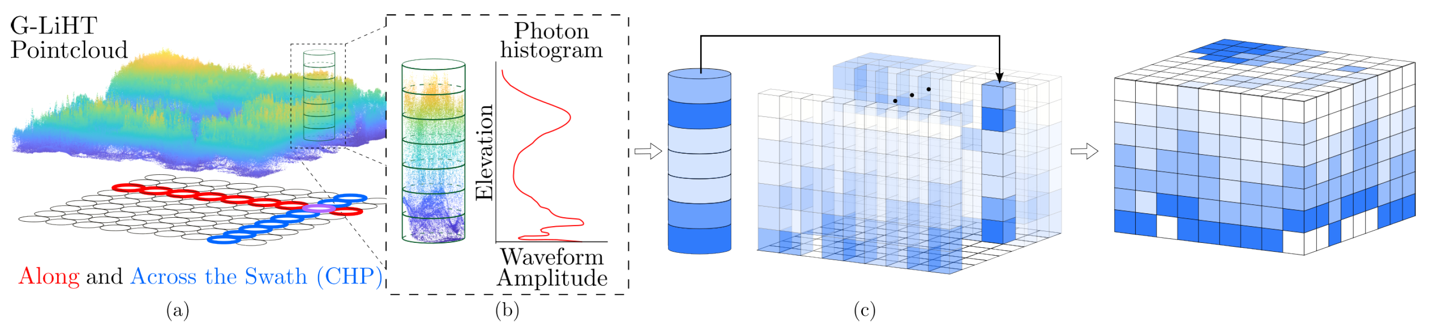
7]. This 3D structure allows researchers to analyze detailed spatial information, making it highly valuable for studying vegetation and terrain and for applying advanced deep learning techniques. To understand how an HHDC is constructed, consider the point cloud shown in
Figure 1a. This point cloud is accompanied by a cylindrical structure with a diameter equivalent to the size of the footprint of a satellite LiDAR shot. By analyzing the vertical distribution of the LiDAR returns within this footprint, we generate a waveform that resembles the elevation histogram typical of waveform LiDAR measurements, as presented in
Figure 1b. By synthesizing similar LiDAR shots both in along-swath and across-swath directions and consolidating them into a single data tensor, we form the HHDC, illustrated in
Figure 1c. The HHDC organizes LiDAR data into a 3D tensor, where the first two dimensions represent the spatial arrangement of laser footprints along and across the swath, while the third dimension captures the vertical structure of the scene, such as canopy height and terrain elevation. This format enables the extraction of biological features, including Canopy Height Models (CHMs), Digital Surface Models (DSMs), and Digital Elevation Models (DEMs). An
voxel of the HHDC represents the number of photons found in the
spatial location and at
height, where
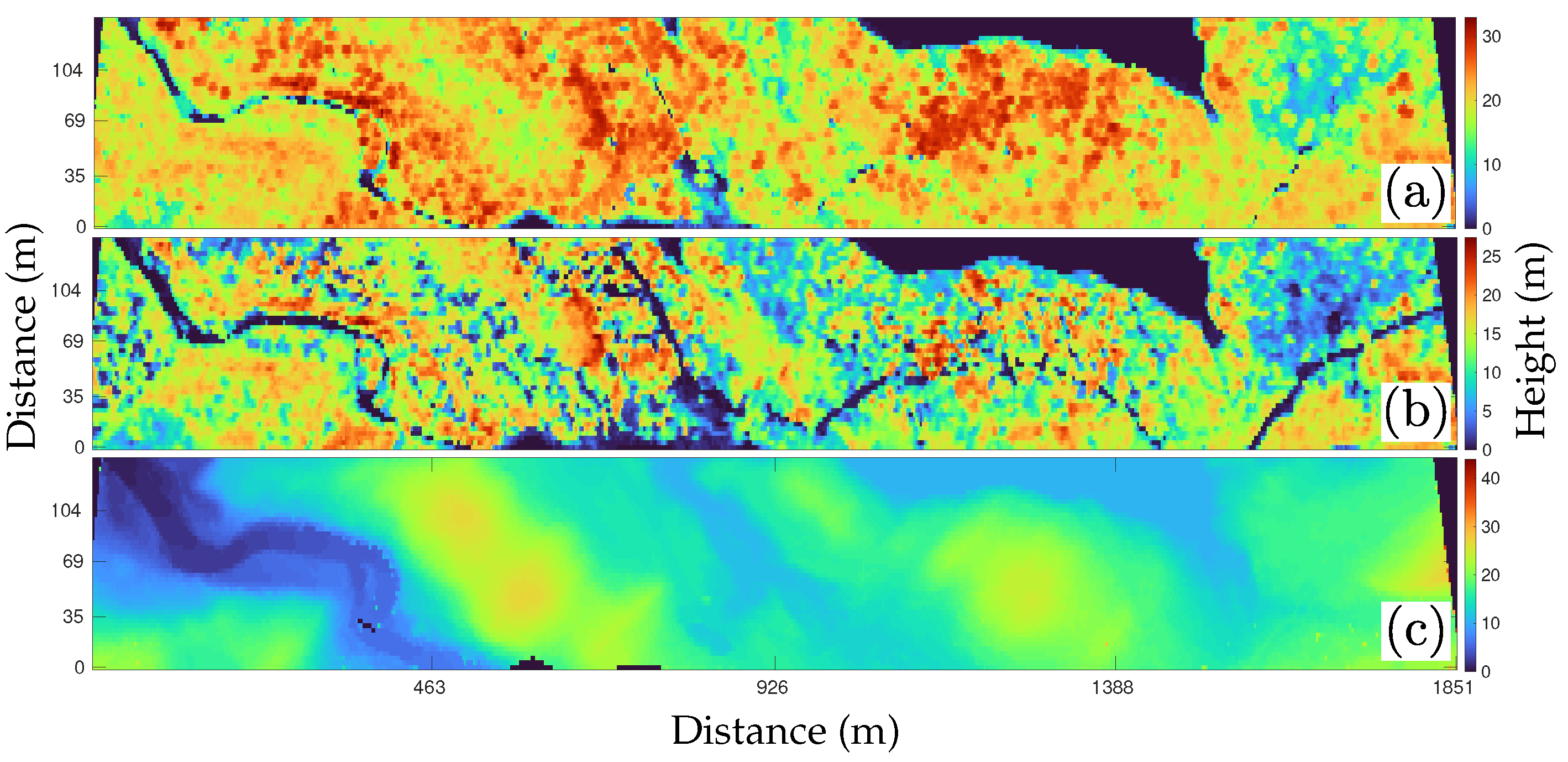
is the vertical resolution. The 2D DTM, for instance, is created as the horizontal slice of the HHDC at the 2% percentile, as shown in
Figure 2c, where the “bare Earth” landscape is clearly seen. The 2D CHM is shown in
Figure 2a and computed as the 98% minus the DTM plane.
Figure 2b shows the 50% that is typically used for biomass studies. As with many signals found in nature, HHDCs present a sparse representation. For instance, 3D wavelet representations of HHDCs of forests and vegetation in Maine show that less than
of the wavelet coefficients are needed to accurately represent the HHDC. This property avails the opportunity to design compressive sensing protocols capable of capturing the essential information content in HHDCs with just a small number of compressive measurements.
3. Bayesian Super-Resolution Framework: Forward Imaging Model and Diffusion Regularization
Satellite LiDAR systems often face limitations in spatial resolution due to constraints in photon density and footprint size. Super-resolution techniques address these limitations by reconstructing a high-resolution representation from sparse low-resolution measurements, thus enhancing spatial detail in LiDAR imaging. This provides a denser and more informative 3D representation that supports detailed environmental analysis. The objective of super-resolution is to recover a high-resolution HHDC,
, from sparse measurements represented by a low-resolution HHDC,
, where
,
, and
. This problem is inherently challenging due to its ill-posed nature: multiple high-resolution representations can map to the same low-resolution measurements. Ref. [
13] formalizes super-resolution within a Bayesian compressed sensing approach, defining a joint probability distribution over both the low-resolution measurements and the high-resolution tensor we aim to recover. Specifically, we consider the joint distribution
, where the goal is to infer the high-resolution tensor,
, given the observed low-resolution measurements,
. By factorizing this joint distribution, we obtain
where
represents the likelihood of observing the low-resolution measurements given a high-resolution representation, describing the distribution governing the LiDAR sensing process.
is the prior over the high-resolution tensor, which encodes prior assumptions about the spatial structure of the high-resolution data. To recover
, we maximize the posterior distribution
, which can be expressed as
Since
is independent of
, maximizing the logarithm of the posterior simplifies to maximizing the joint likelihood and prior terms. Thus, Ref. [
13] formulates the super-resolution task as the following optimization problem:
where
is the data fidelity term, derived from the likelihood and represented by the Kullback–Leibler divergence between the observed measurements
and the predicted measurements
. Here,
denotes the forward imaging model of the satellite LiDAR, enhanced with a randomized illumination pattern
. The illumination pattern
plays a crucial role in enabling a compressed representation of the high-resolution HHDC. Instead of targeting specific regions,
introduces random variations into the illumination process. This randomness ensures the incoherence property that is essential for compressed sensing, which allows the system to efficiently capture and reconstruct the necessary information from fewer measurements. By spreading the measurement energy uniformly across the data space, we preserve essential details without requiring a dense sampling of the entire scene. This approach not only reduces the volume of data needed for accurate reconstruction but also simplifies the design and operation of the illumination system. Consequently, incorporating
into the forward model
aligns our methodology with compressed sensing principles, facilitating efficient recovery of
(as discussed further in
Section 3.1 and
Section 4).
The term
serves as a regularization term, integrating prior knowledge to encourage plausible high-resolution structures (detailed in
Section 3.2). By combining the data fidelity term and the regularization term, the optimization process effectively reconstructs
while balancing adherence to observed data and the incorporation of prior information.
3.1. Forward Imaging Model for Data Fidelity
The data fidelity term
is computed using a forward imaging model,
, which probabilistically describes the sensing process of the satellite LiDAR system. Given a high-resolution HHDC
, the forward model
outputs a distribution over low-resolution measurements, capturing the process that reduces spatial resolution through factors such as footprint size, Gaussian convolution, and photon loss. Formally, Ref. [
13] models
as being distributed according to
where
r represents the number of photons returning to the satellite per footprint and
is a Gaussian kernel characterizing the footprint dimensions. To implement the forward model enhanced with an illumination pattern
, it is necessary to capture three key phenomena in the LiDAR sensing process (as depicted in
Figure 3):
Gaussian Beam Convolution: In satellite LiDAR, the laser shots exhibit a Gaussian beam pattern, which defines the footprint on the ground. This footprint’s energy distribution is modeled by a Gaussian convolution with the high-resolution data. The Gaussian kernel
is defined by its Full Width at Half Maximum (FWHM) and the footprint radius at which the intensity drops to
. The 2D Gaussian filter
used to model footprint aggregation is expressed as
where
i and
j are the integer indices of the kernel,
k is its size, and
. This convolutional operation aggregates neighboring high-resolution footprints, reducing spatial resolution while capturing the Gaussian spread of each footprint.
Photon Loss with Distance—Multinomial Distribution: As the distance between the satellite and the ground increases, the number of photons returning to the detector decreases, leading to a reduction in photon count within each footprint. This phenomenon is modeled by a multinomial distribution, where the number of detected photons
r in each footprint is distributed based on the energy received from each altitude bin. Given a high-resolution footprint histogram, the low-resolution photon counts are obtained by sampling from a multinomial distribution:
where
is the photon count in each bin,
is the normalized probability for each bin, and
c is the number of vertical bins. This model captures the stochastic nature of photon loss with increasing satellite altitude, reflecting the distribution of detected photons in low-resolution measurements.
Illumination Pattern: To enhance data compression and ensure incoherence, an illumination pattern is incorporated into the forward model . The pattern represents a randomized selection of low-resolution footprints, distributing the illumination energy in a manner consistent with principles from compressed sensing. This randomization ensures that the measurements exhibit incoherence, a key property for accurate recovery in under-sampled systems. Unlike explicitly selective approaches, this randomized strategy simplifies the implementation while still preserving critical information required for reconstructing high-resolution structures within . By applying , the model achieves effective compression by capturing essential data elements without the need for a fully dense or adaptively designed sampling strategy, thereby reducing the overall data volume while maintaining reconstruction fidelity.
Together, these processes define , allowing us to compute the data fidelity term .
To incorporate the illumination pattern into the forward model , we implement as a randomized binary mask applied to the low-resolution footprint grid. Each element in is independently set to 1 with probability p (e.g., ), indicating that the corresponding footprint is illuminated and measured, and to 0 otherwise. This random selection of footprints ensures that the measurements are incoherent with the sparse representation of the high-resolution HHDC in some domain (e.g., Fourier or wavelet), a critical requirement for compressed sensing. By distributing the sampling randomly across the scene, captures a diverse set of measurements that enable accurate reconstruction of from fewer data points. This approach simplifies the onboard implementation compared to adaptive sampling strategies, which may demand complex hardware or prior scene knowledge, while still providing the necessary mathematical guarantees for recovery.
The use of a randomized illumination pattern
is grounded in the principles of compressed sensing, where random sampling ensures incoherence with the sparse basis (e.g., wavelets) of the HHDC, enabling accurate reconstruction from a reduced number of measurements. This randomness satisfies the restricted isometry property (RIP) with high probability, providing universal recovery guarantees for any sparse signal without requiring prior knowledge of its sparsity pattern. In contrast, adaptive or optimized sampling strategies tailor the illumination to specific signal characteristics, potentially reducing the number of measurements further (e.g., by 20–50% for highly structured scenes, based on prior studies like [
14]), but at the cost of increased complexity. For satellite LiDAR, where robustness across diverse unknown terrains and hardware simplicity are paramount, the randomized approach offers consistent performance without the need for real-time adaptation or sophisticated onboard processing. While adaptive methods might lower sampling rates for specific scenes, the randomized pattern’s simplicity and universality make it well suited for global Earth observation under operational constraints.
3.2. Diffusion Models for Regularization
To enforce the regularization term −
, we employ diffusion generative models [
18,
19,
20]. This formulation not only provides a powerful probabilistic prior for high-resolution HHDCs but also constrains the solution space of our compressed sensing problem, allowing the optimization algorithm to sample exclusively from the distribution of high-resolution data learned by the diffusion model. The SDE-based diffusion model consists of two main processes (as depicted in
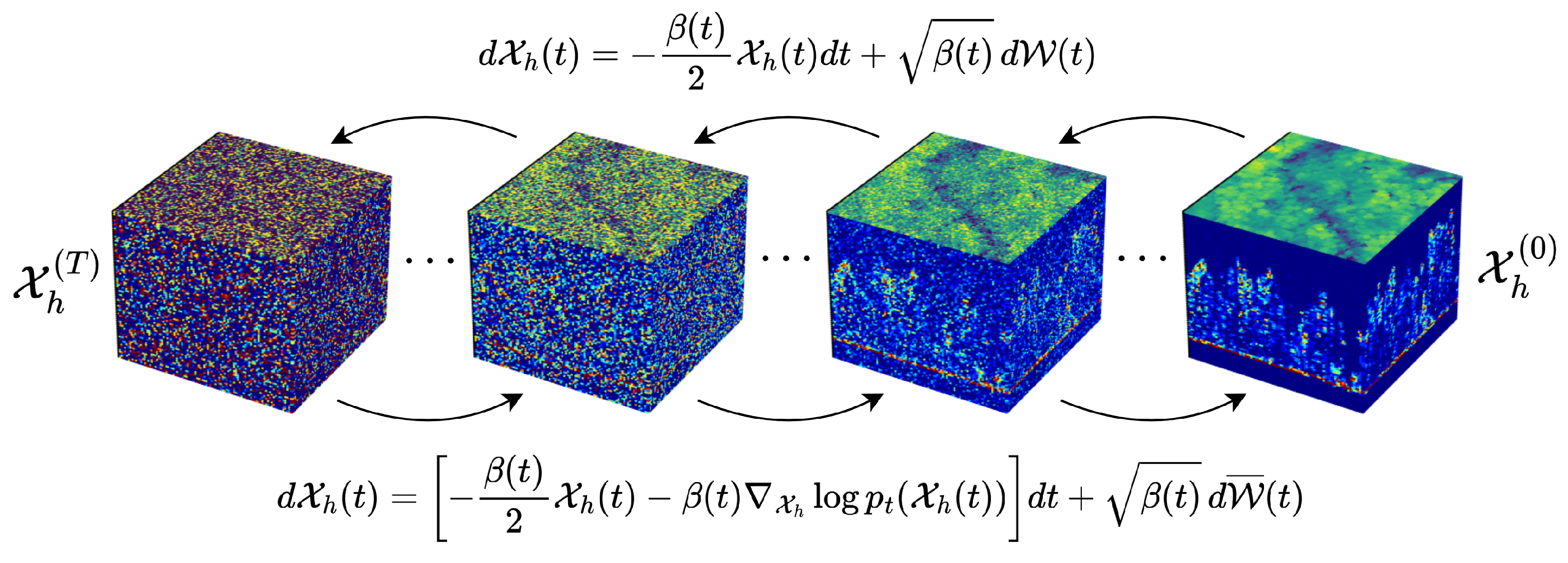
Figure 4): a forward diffusion process that progressively corrupts data by adding noise and a reverse diffusion process that undoes this noise, ultimately sampling from a distribution that closely matches the high-resolution data. The SDE framework offers continuous control over noise injection and removal, making it highly suitable for guiding the compressed sensing optimization.
3.2.1. Forward Diffusion Process
The forward diffusion process (
Figure 4-top) is modeled as a stochastic differential equation (SDE) that gradually transforms a clean high-resolution tensor
into pure noise over continuous time
. Ref. [
19] represents this process as
where
is the drift term, governing deterministic changes in
over time
t,
is the diffusion coefficient that scales the noise added at each instant, and
is an increment of a Wiener process. In the variance-preserving (VP) framework [
19], we set the drift term as
where
is the noise schedule that controls the rate of variance addition over time. This drift term pulls
toward zero, effectively centering the distribution of
as noise increases. The diffusion coefficient
, which scales the noise, is given by
The schedule
is typically chosen as an increasing function of
t, ensuring that the injected noise grows over time. Common choices for
include linear and cosine schedules, both of which enable a smooth transition from structured data to pure Gaussian noise. At
, we begin with a sample
drawn from the high-resolution data distribution
. As
t approaches
T,
converges to a known prior noise distribution, forming a flexible and stable framework for diffusion-based generative modeling. For the remainder of this paper, we adopt this variance-preserving (VP) approach, with the defined drift and diffusion terms, to control variance throughout the forward diffusion process. In our implementation, we employed a linear noise schedule for
, where
increases linearly from
to
over
diffusion steps, consistent with the standard practice in Denoising Diffusion Probabilistic Models (DDPMs) [
18], as will be described in
Section 4.1. This schedule ensures a gradual increase in noise during the forward process, facilitating a smooth transition from the high-resolution HHDC distribution to a pure Gaussian noise distribution. We chose this linear schedule for its simplicity and proven effectiveness in generative modeling tasks, such as image generation, which shares similarities with our task of reconstructing detailed forest landscapes from sparse LiDAR measurements. The choice of
steps balances computational efficiency with the ability to capture fine-grained details in the reverse diffusion process, while the range of
values ensures that the model learns to denoise effectively across all stages of corruption.
3.2.2. Reverse Diffusion Process
To reconstruct high-resolution data from noise, we define a reverse-time stochastic differential equation (SDE) that progressively removes the noise added during the forward process (
Figure 4-bottom). According to Anderson’s theorem [
21], the reverse diffusion process, which generates samples from the high-resolution distribution, can be expressed as
where
is the score function, representing the gradient of the log probability density of
at time
t. This term encourages the process to move in directions that increase the likelihood of high-resolution data, effectively constraining the solution to realistic high-resolution HHDC representations.
is a Wiener process in reverse time, effectively “undoing” the stochastic increments of the forward process. This reverse SDE guides
from pure Gaussian noise at
back to a high-resolution sample at
. By incorporating the score function
, the model is able to infer the structure in high-resolution data, making it more likely to produce realistic samples. This gradient-based component, weighted by the schedule
, effectively constrains the sampling process to lie within the distribution of high-resolution data while following the forward process’s variance-preserving setup. This combination of drift and score-guided diffusion provides a smooth and effective path back to high-resolution data.
4. Solving the Inverse Problem via Posterior Sampling
In the framework of satellite LiDAR super-resolution, solving the inverse problem is formulated as sampling from the posterior distribution
, as defined in Equation (
2). Leveraging the diffusion model in this process, we iteratively refine the high-resolution estimate
by directing the reverse diffusion with the posterior score function,
. This guidance enables the diffusion process to navigate toward configurations that are consistent with both the observed data and our prior knowledge. By Bayes’ rule, the posterior score can be decomposed as
where
represents the score of the likelihood term. This term enforces data fidelity by aligning the reconstructed high-resolution data
with the observed low-resolution measurements
. Notably, this score is inherently linked to the KL divergence term in Equation (
3),
, where minimizing the KL divergence effectively maximizes the likelihood
, ensuring that
closely matches
. The second term,
, is the score of the prior distribution, encoding structural assumptions about
that are enforced by the diffusion process. This term constrains the solution space, directing the optimization to sample from the high-resolution data distribution learned by the diffusion model. Combining both terms in the posterior score enables a high-resolution reconstruction that aligns with observed data while respecting the priors imposed by the diffusion process, ultimately finding the optima for Equation (
3).
However, directly computing the likelihood term at each optimization step is computationally expensive as it requires a complete reverse diffusion process. Each step in this process involves multiple neural network evaluations to iteratively denoise the high-resolution tensor
, which becomes prohibitive for real-time or large-scale applications. To mitigate this, Ref. [
22] proposed Diffusion Posterior Sampling (DPS), which approximates the posterior using Tweedie’s formula [
23]. This formula provides an estimate of the fully denoised HHDC based on the observed noisy sample, approximating the posterior mean without requiring a full denoising at each iteration. Specifically, for an intermediate noisy sample
at time
t, Tweedie’s formula estimates the clean fully denoised tensor
as
where
is a time-dependent scaling factor, and
is the score function approximated by the pre-trained diffusion model. This estimate enables the posterior sampling process to bypass the costly neural network evaluations for a full reverse diffusion pass by using the denoised tensor to efficiently compute the likelihood term. Our key contribution modifies DPS to enhance its accuracy by replacing the original norm-based optimization with the gradient of the KL divergence term that uses an illumination pattern
, achieving efficient posterior sampling guided by data fidelity and high-resolution priors. By iteratively applying this approximation, DPS with the KL divergence term efficiently samples from
, reconstructing a high-resolution HHDC that is both consistent with the low-resolution sparsely sampled observations and constrained by learned high-resolution priors.
4.1. Algorithm Implementation
As described in
Section 3.2.1, we adopt the variance-preserving (VP) framework for diffusion models. To implement this framework algorithmically, a discretized version of Equation (
5) is required. For this purpose, we divide the time domain into
N discrete bins and define
, representing the state at the
i-th time step. The noise schedule at the
i-th step is denoted as
. Following the framework of DDPM [
18], we set
, which represents the complementary noise weight. The cumulative product of noise weights up to the
i-th step is given by
. Additionally, we define
, which plays a crucial role in characterizing the variance during the reverse diffusion process. This discretization forms the foundation for the numerical implementation of the diffusion process. With these definitions, we implement our modified version of DPS as outlined in Algorithm 1. The key modification—incorporating the illumination pattern into the KL divergence—is highlighted in
purple, providing a clear distinction of our contributions.
| Algorithm 1 Diffusion Posterior Sampling [22] with KL divergence and illumination pattern. |
- Require:
N, , , - 1:
- 2:
for to 0 do - 3:
▹ Estimation of using a neural network. - 4:
- 5:
- 6:
- 7:
- 8:
end for - 9:
return:
|
4.2. Need for Quality Assessment of Reconstructed Data
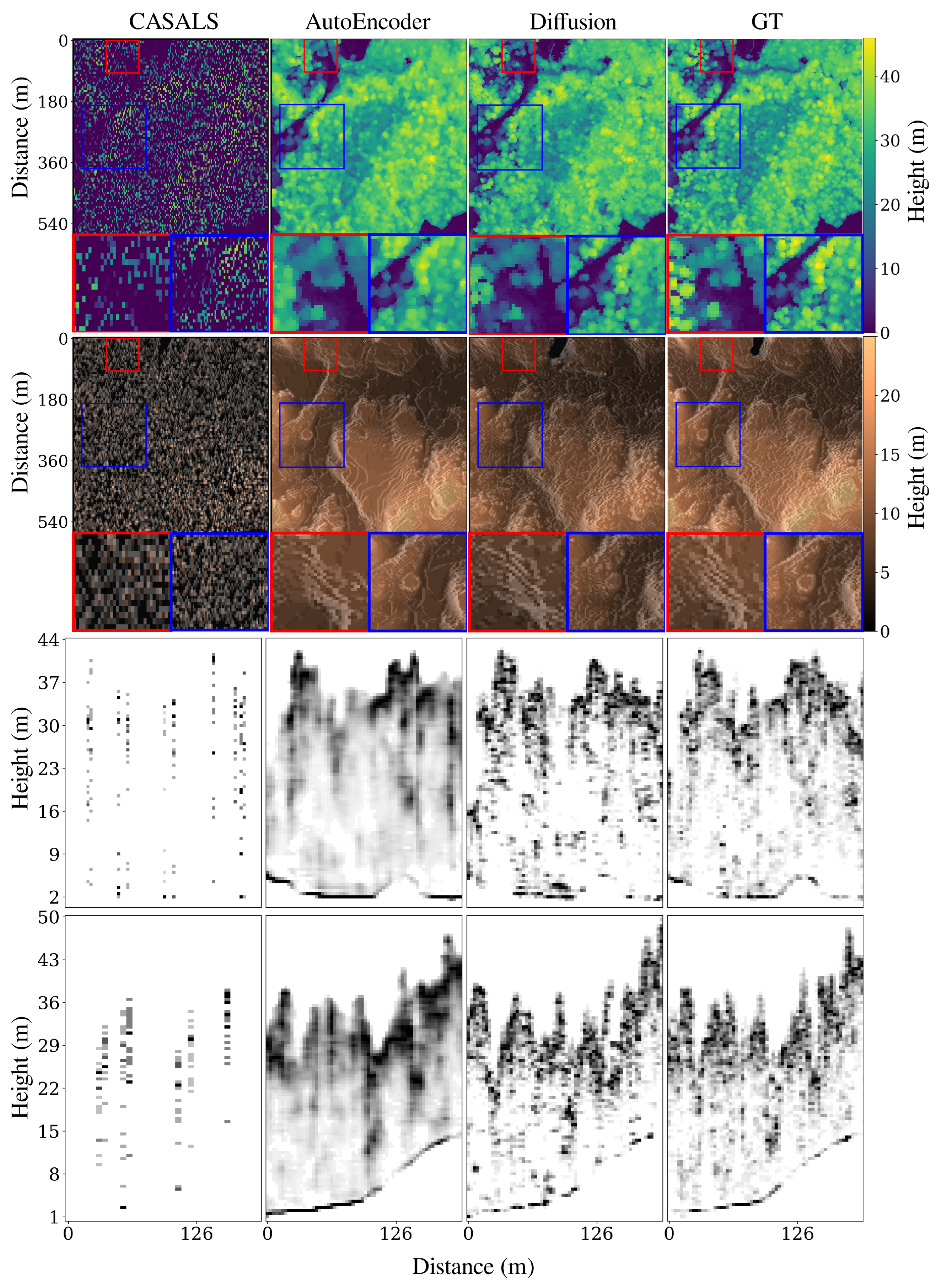
While our diffusion-based reconstruction algorithm demonstrates promising results in super-resolving HHDCs from sparse measurements (as will be shown in
Section 6), it is imperative to evaluate the quality and reliability of the reconstructed data. The inherent lossy nature of the compression and reconstruction process can introduce deviations from the ground truth, potentially impacting downstream applications such as ecological modeling and biomass estimation. Therefore, a thorough analysis using image quality assessment (IQA) metrics is necessary to quantify the fidelity of the reconstructed HHDCs and ensure their suitability for practical use. In the following sections, we delve into the evaluation of various IQA metrics to assess their effectiveness in capturing the quality of reconstructed forest landscapes.
5. Evaluating Image Quality Metrics for Reconstructed LiDAR Data
Building upon the necessity to evaluate the reconstructed Hyperheight Data Cubes (HHDCs), we explore the suitability of existing image quality assessment (IQA) metrics for our application. IQA metrics play a vital role in quantifying the perceptual and structural fidelity of reconstructed images compared to the ground truth. In the context of LiDAR data and HHDCs, it is essential to identify metrics that accurately reflect the quality of the reconstructed 3D representations. This section presents a preliminary verification of various full-reference IQA metrics to determine their applicability and effectiveness in assessing the quality of forest landscapes reconstructed from compressed LiDAR data.
The task at hand, i.e., estimating the quality of forest landscapes reconstructed from LiDAR data, is relatively novel. Previous publications [
11] on this topic have predominantly relied on metrics such as Mean Absolute Error (MAE), Mean Squared Error (MSE), and Structural Similarity (SSIM) [
24] to characterize and compare the performance of various reconstruction techniques. However, these metrics may not be the most suitable for this specific application, and incorporating additional metrics of a different nature could prove beneficial. This assertion is supported by two main considerations. Firstly, MSE (or, equivalently, PSNR) is highly correlated with SSIM [
25], making the simultaneous use of both metrics redundant. Secondly, while these metrics are still widely employed across many image processing applications, a significant number of newly proposed full-reference and no-reference visual quality metrics have demonstrated efficacy in alternative contexts [
26], suggesting their potential utility in this domain.
Identifying efficient and adequate metrics for compressive sensing and related applications, such as sparse reconstruction, is of particular interest. Commonly used criteria include recovery success rate, reconstruction error, recovery time, compression ratio, and processing time [
27]. However, in our case, recovery and processing time are not of primary concern. The work in [
28] explores the use of no-reference metrics and introduces the CS Recovered Image Quality (CSRIQ) metric, which measures both local and global distortions in recovered data. Subjective assessments of restored image quality are thoroughly investigated across several databases in [
29], where it is shown that the Codebook Representation for No-Reference Image Assessment (CORNIA) metric [
30] performs well for sparse reconstruction. Additionally, Ref. [
31] examines several full-reference quality metrics for image inpainting, noting that the most effective metrics, achieving Spearman’s rank-order correlation coefficient (SROCC) with Mean Opinion Score (MOS) values exceeding 0.9, are not widely adopted for characterizing other types of distortions.
Thus, we decided to conduct an initial analysis of existing metrics’ properties using the Tampere Image Database (TID2013) as it includes data for distortion #24—image reconstruction from sparse data [
32]. This part of the database comprises 25 test images with five levels of distortion corresponding to PSNR values of approximately 33, 30, 27, 24, and 21 dB. Notably, PSNR = 33 dB corresponds to almost invisible distortions, also referred to as just-noticeable distortions (JND) [
33], whereas PSNR = 21 dB represents distortions that are generally considered annoying. The other cases lie between these extremes.
Although the method of sparse reconstruction employed in TID2013 differs from that used for forest landscape reconstruction, which is highly specific, we believe that visual quality metrics based on the human visual system (HVS) can be valuable. These metrics account for features such as edge, detail, and texture preservation more effectively than PSNR or SSIM. This consideration is particularly relevant for forest landscapes, where sharp transitions and textures are common and must be preserved during the reconstruction process.
A good metric is expected to exhibit a high rank-order correlation with MOS, which represents the average subjective quality assessment from multiple participants. This assumption has been validated across numerous applications [
34]. Consequently, higher Spearman’s rank-order correlation coefficient (SROCC) values serve as strong evidence for a metric’s suitability in specific applications (when calculated for images with certain distortion types) or its general applicability (when calculated across various distortion types in TID2013 or similar databases).
We calculated SROCC values for three groups of images:
Images with sparse sampling only, to identify the most effective metrics for this case and lay the foundation for further analysis;
Images with sparse reconstruction combined with additive white Gaussian noise, assuming noise may be present in our data;
Images with sparse reconstruction and lossy compression, to evaluate metrics that perform well when data are compressed and subsequently reconstructed.
It is important to emphasize that the obtained results do not guarantee that the behavior of metrics in the context of our specific application will exactly match their performance on the color image database. Nevertheless, these findings provide a preliminary heuristic foundation for further investigation.
Recall that all distortion types in the TID2013 database are assigned dedicated indices.
Table 1 lists the distortion types relevant to this study. We computed SROCC values for three groups of distortions as follows:
#24—to focus exclusively on sparse sampling distortions;
#1 and #24—to compare the adequacy of sparse sampling distortions (type 24) with additive white Gaussian noise (type 1), which is the most commonly considered distortion type for quality metrics;
#10, #11, #21, and #24—to jointly analyze sparse reconstruction and distortions arising from lossy compression.
It is worth noting that, for most visual quality metrics, higher values indicate better quality (e.g., PSNR or SSIM). However, some metrics are designed such that smaller values correspond to better quality. In these cases, SROCC is negative and should approach −1.
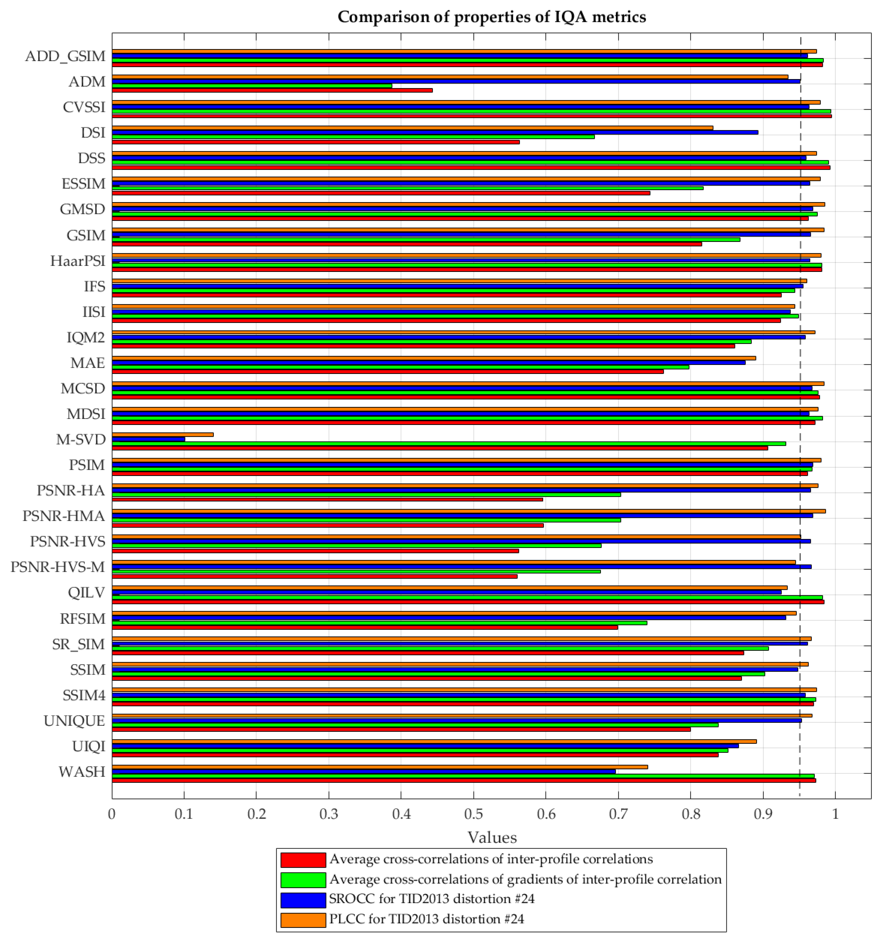
We evaluated 60 full-reference metrics, and the resulting SROCC values are presented in
Table 2. Additionally, Pearson’s linear correlation coefficients (PLCCs) were computed for distortion type #24, as well as for two other groups of the TID2013 subsets mentioned above, using a nonlinear fitting function derived from the entire TID2013 dataset. This fitting approach, recommended by the Video Quality Experts Group (VQEG), is widely used in image quality assessment to account for the nonlinear characteristics of the human visual system (HVS).
Before starting data analysis, some preliminary comments are needed. In general, it is difficult to obtain SROCC larger than 0.98 due to the limited number of experiment participants and the diversity in their opinions. Hence, SROCC values equal to 0.97 or even 0.96 can be treated as excellent results. Then, the following conclusions can be drawn:
there are numerous metrics that produce better results than PSNR and SSIM;
the best of them are GMSD, MCSD, HaarPSI, PSIM, PSNR-HMA (description below), and some others for various subsets; we can decide what metrics to choose for further use;
there are other factors that can influence the choice of appropriate metric; for example, most metrics analyzed above are suited for characterizing the visual quality of color images, but we have data arrays more similar to grayscale images; then, such metrics as PSNR-HMA can be replaced by PSNR-HVS-M;
the metric’s computational efficiency is not important for the considered application since the metric is used for quality characterization but not in the image processing loop;
usually, if a given visual quality metric shows that image/data quality is good, then the results of parameter estimation for such data are good as well;
metrics have different ranges of their variation: some of them are expressed in dB, and others are in the limits from 0 to 1; because of this, it is necessary to consider these peculiarities in the analysis of data based on calculated metrics.
Most of the best metrics originate from the SSIM idea; however, they are calculated using additional image preprocessing and/or transforms. For example, Gradient Magnitude Similarity Deviation (GMSD) [
37] utilizes global variation regarding gradient-based local quality maps, assuming the use of the Prewitt filter to determine the local gradient values. Then, the gradient similarity map is obtained using a formula similar to the SSIM calculation. The idea of Multiscale Contrast Similarity Deviation (MCSD) [
38] is based on the calculation of contrast similarity deviations for three scales and further pooling using their weighted product. The contrast similarity between two compared images is also calculated using the SSIM-like formula. Both of these metrics are also characterized by relatively low computational complexity.
The Perceptual Similarity (PSIM) metric [
35] extracts the gradient magnitude maps using the Prewitt filter, which are then compared using the multiscale similarity computation, further subject to perceptual pooling. As in the previously mentioned metrics, the similarity measure applied for the detection of differences between the gradient magnitude maps of the assessed image and the reference one is similar to the original SSIM formula.
Another computationally inexpensive metric, namely Haar wavelet-based Perceptual Similarity Index (HaarPSI) [
44], is based on the wavelet decomposition conducted using six two-dimensional Haar filters. The coefficients obtained are compared to determine the local similarities and the importance of particular regions of the image. This metric takes into account such a feature of human vision as human attention or saliency, and this can be the reason why it is among the best. It should also be noted that most of the best metrics utilize gradient information in some way or another.
Nevertheless, the PSNR-HMA metric [
36], also listed as one of the best metrics, has a different “nature” since it is a modification of the simple Peak Signal to Noise Ratio (PSNR) with additional use of Contrast Sensitivity Function (CSF) between-coefficient contrast masking of DCT basis functions, as well as mean shift and contrast changing.


 ,
, 


